Efficient computation of oriented vertex and arc colorings of special digraphs

Abstract

In this paper we study the oriented vertex and arc coloring problem on edge series-parallel digraphs (esp-digraphs) which are related to the well known series-parallel graphs. Series-parallel graphs are graphs with two distinguished vertices called terminals, formed recursively by parallel and series composition. These graphs have applications in modeling series and parallel electric circuits and also play an important role in theoretical computer science. The oriented class of series-parallel digraphs is recursively defined from pairs of vertices connected by a single arc and applying the parallel and series composition, which leads to specific orientations of undirected series-parallel graphs. Further we consider the line digraphs of edge series-parallel digraphs, which are known as minimal series-parallel digraphs (msp-digraphs).

We show tight upper bounds for the oriented chromatic number and the oriented chromatic index of edge series-parallel digraphs and minimal series-parallel digraphs. Furthermore, we introduce first linear time solutions for computing the oriented chromatic number of edge series-parallel digraphs and the oriented chromatic index of minimal series-parallel digraphs.

Keywords: Edge series-parallel digraphs; Minimal series-parallel digraphs; Oriented vertex-coloring; Oriented arc-coloring; Linear time solutions

1 Introduction

A homomorphism from an oriented graph $G=(V_{G},E_{G})$ to an oriented graph $H=(V_{H},E_{H})$ is an arc preserving mapping $h$ from $V_{G}$ to $V_{H}$, i.e. if $(u,v)\in E_{G}$ then $(h(u),h(v))\in E_{H}$.

An oriented $r$-vertex-coloring of an oriented graph $G$ corresponds to an oriented graph $H$ on $r$ vertices, such that there exists a homomorphism from $G$ to $H$. The oriented chromatic number of $G$, denoted by $\chi_{o}(G)$, is the minimum number of vertices in an oriented graph $H$ such that there is a homomorphism from $G$ to $H$.

In the Oriented Chromatic Number problem (OCN for short) there is given an oriented graph $G$ and an integer $r$ and we have to decide whether there is an oriented $r$-vertex-coloring for $G$. If $r$ is constant, i.e. not part of the input, the corresponding problem is denoted by $\text{OCN}_{r}$. Even $\text{OCN}_{4}$ is NP-complete [CD06].

Moreover, an oriented $r$-arc-coloring of an oriented graph $G$ relates to an oriented graph $H$ on $r$ vertices, such that there is a homomorphism from line digraph $LD(G)$ to $H$. The oriented chromatic index of $G$, denoted by $\chi^{\prime}_{o}(G)$, is the minimum number of vertices in an oriented graph $H$ such that there is a homomorphism from line digraph $LD(G)$ to $H$.

In the Oriented Chromatic Index problem (OCI for short) there is given an oriented graph $G$ and an integer $r$ and we have to decide whether there is an oriented $r$-arc-coloring for $G$. If $r$ is constant, i.e. not part of the input, the corresponding problem is denoted by $\text{OCI}_{r}$. Even $\text{OCI}_{4}$ is NP-complete [OPS08].

The hardness of $\text{OCN}_{4}$ and $\text{OCI}_{4}$ motivates to consider the oriented chromatic number and the oriented chromatic index of special graph classes. This was frequently done for undirected graphs, where the maximum value $\chi_{o}(G^{\prime})$ or $\chi^{\prime}_{o}(G^{\prime})$ of all possible orientations $G^{\prime}$ of a graph $G$ is considered, see [DS14, Mar13, Mar15, OP14, Sop97] and [OPS08, PS06]. In this sense it has been shown in [Sop97] that every series-parallel graph has oriented chromatic number at most $7$ and that this bound is tight. Since the oriented chromatic index is always less or equal the oriented chromatic number (Observation 2.7) every series-parallel graph has oriented chromatic index at most $7$ and by [PS06] this bound is also tight.

In this paper we consider the oriented chromatic number and the oriented chromatic index of esp-digraphs (short for edge series-parallel digraphs) which can recursively be defined from the single edge graph by applying the parallel composition and series composition. and lead to specific orientation of series-parallel graphs. Further, we consider the oriented chromatic number and the oriented chromatic index of line digraphs of edge series-parallel digraphs, which are known as msp-digraphs (short for minimal series-parallel digraphs) and can recursively be defined from the single vertex graph by applying the parallel composition and series composition. The classes of msp-digraphs and esp-digraphs are incomparable in terms of set inclusion (Remark 4.6).

As every esp-digraph is a specific orientation of a series-parallel graph the mentioned bounds for series-parallel graphs lead to (not necessarily tight) upper bounds for the oriented chromatic number and the oriented chromatic index of esp-digraphs.

In this paper we re-prove the bound of $7$ for the oriented chromatic number and the oriented chromatic index of esp-digraphs and we show that these bounds are tight even for esp-digraphs. Since the oriented chromatic index of esp-digraphs equals the oriented chromatic number of their line digraphs, namely msp-digraphs, we obtain a tight upper bound of $7$ for the oriented chromatic number of msp-digraphs. Further, (by Observation 2.7) this leads to an upper bound of $7$ for the oriented chromatic index of msp-digraphs. We give an example that this bound is best possible.

We also consider solutions for computing the oriented chromatic number and the oriented chromatic index of esp-digraphs and msp-digraphs. In [GKL20] we gave a first linear time solution for computing the oriented chromatic number of msp-digraphs. Using the line digraphs this leads to a linear time solution for computing the oriented chromatic index of esp-digraphs. In this paper we introduce linear time solutions for computing the oriented chromatic number of esp-digraphs and the oriented chromatic index of msp-digraphs.

In Tables 1 and 2 we summarize these results.

$G$	$\chi_{o}(G)\leq 7$	sharpness	recognition
esp-digraph	Theorem 3.15 or Corollary 3.14	Example 3.16	$\text{$\mathcal{O}$}(n+m)$	Theorem 3.19
msp-digraph	[GKL20] or Remark 4.9	Example 4.10	$\text{$\mathcal{O}$}(n+m)$	[GKL20]

Table 1: Oriented chromatic number $\chi_{o}$ of msp-digraphs and esp-digraphs

$G$	$\chi^{\prime}_{o}(G)\leq 7$	sharpness	recognition
esp-digraph	Remark 3.11 or Corollary 3.10	Example 3.12	$\text{$\mathcal{O}$}(n+m)$	Corollary 3.13
msp-digraph	Corollary 4.12	Example 4.13	$\text{$\mathcal{O}$}(n+m)$	Theorem 4.20

Table 2: Oriented chromatic index $\chi^{\prime}_{o}$ of msp-digraphs and esp-digraphs

2 Preliminaries

2.1 Graphs and digraphs

We refer to the notations of Bang-Jensen and Gutin [BJG09] for (di)graphs. A graph is a pair $G=(V,E)$ with a finite set $V$ of vertices and a finite set of edges $E\subseteq\{\{u,v\}\mid u,v\in V,~{}u\not=v\}$. We call a pair $G=(V,E)$ directed graph or digraph, such that $V$ is a finite set of vertices and $E\subseteq\{(u,v)\mid u,v\in V,~{}u\not=v\}$ is a finite set of ordered pairs of distinct vertices called arcs or directed edges. For a vertex $v\in V$, we define the sets $N^{+}(v)=\{u\in V\mid(v,u)\in E\}$ and $N^{-}(v)=\{u\in V\mid(u,v)\in E\}$ as the set of all successors and the set of all predecessors of vertex $v$. The outdegree of $v$, $\text{outdegree}(v)$ for short, is the number of successors of $v$ and analogously the indegree of $v$, $\text{indegree}(v)$ for short, is the number of predecessors of $v$.

Digraph $G^{\prime}=(V^{\prime},E^{\prime})$ is called a subdigraph of digraph $G=(V,E)$ if $V^{\prime}\subseteq V$ and $E^{\prime}\subseteq E$ holds. Moreover, $G^{\prime}$ is an induced subdigraph of $G$, denoted by $G^{\prime}=G[V^{\prime}]$ if every arc of $E$ with both end vertices in $V^{\prime}$ exists in $E^{\prime}$.

For a digraph $G=(V,E)$ its underlying undirected graph is defined by disregarding the directions of the arcs, i.e., ${\it un}(G)=(V,\{\{u,v\}\mid(u,v)\in E,u,v\in V\})$.

For an undirected graph $G=(V,E)$ replacing every edge $\{u,v\}$ of $G$ by exactly one of the arcs $(u,v)$ and $(v,u)$ leads to an orientation of $G$. Every digraph that can be obtained by an orientation of an undirected graph $G$ is called an oriented graph, i.e., an oriented graph is a digraph without loops or opposite arcs.

A tournament is a digraph with exactly one arc between every two distinct vertices. A digraph in which there are no directed cycles is called directed acyclic graph (DAG for short). The girth of digraph $G$ is defined by the length (number of arcs) of a shortest directed cycle in $G$. For a DAG $G$ the girth is defined to be infinity.

The line digraph $LD(G)$ of digraph $G$ has a vertex for every arc in $G$ and an arc from $u$ to $v$ if and only if $u=(x,y)$ and $v=(y,z)$ for vertices $x,y,z$ from $G$ [HN60]. We call digraph $G$ the root digraph of $LD(G)$.

2.2 Undirected vertex-colorings

Definition 2.1 (Vertex-coloring)

An $r$-coloring of a graph $G=(V,E)$ is a mapping $c:V\to\{1,\ldots,r\}$ such that:

• $c(u)\neq c(v)$ for every $\{u,v\}\in E$.

The chromatic number of $G$, denoted by $\chi(G)$, is the smallest $r$ such that $G$ has an $r$-coloring.

We consider the following problem.

• Chromatic Number (CN)

• A graph $G=(V,E)$ and a positive integer $r\leq|V|$.

• Is there an $r$-coloring for $G$?

If $r$ is a constant and not part of the input, the corresponding problem is denoted by $r$-Chromatic Number ($\text{CN}_{r}$). Even on 4-regular planar graphs $\text{CN}_{3}$ is NP-complete [Dai80].

It is well known that bipartite graphs are exactly the graphs which allow a 2-coloring and that planar graphs are graphs that allow a 4-coloring. On undirected co-graphs, the graph coloring problem can be solved in linear time [CLSB81].

2.3 Oriented vertex-colorings

In 1994 Courcelle [Cou94] introduced oriented graph coloring, which considers only oriented graphs.

Definition 2.2 (Oriented vertex-coloring [Cou94])

An oriented $r$-vertex-coloring of an oriented graph $G=(V,E)$ is a mapping $c:V\to\{1,\ldots,r\}$ such that:

• $c(u)\neq c(v)$ for every $(u,v)\in E$,

• $c(u)\neq c(y)$ for every two arcs $(u,v)\in E$ and $(x,y)\in E$ with $c(v)=c(x)$.

The oriented chromatic number of $G$, denoted by $\chi_{o}(G)$, is the smallest $r$ such that there exists an oriented $r$-vertex-coloring for $G$. Then $V_{i}=\{v\in V\mid c(v)=i\}$, $1\leq i\leq r$ is a partition of $V$, which we call color classes.

For two digraphs $G_{1}=(V_{1},E_{1})$ and $G_{2}=(V_{2},E_{2})$, a homomorphism from $G_{1}$ to $G_{2}$ is a mapping $h:V_{1}\to V_{2}$, which preserves the edges, i.e., $(u,v)\in E_{1}$ implies $(h(u),h(v))\in E_{2}$.

A homomorphism from $G_{1}$ to $G_{2}$ can be regarded as an oriented coloring of $G_{1}$ in which the vertices of $G_{2}$ can be seen as color classes. Thus, we call $G_{2}$ the color graph of $G_{1}$. This leads to equivalent definitions for the oriented coloring and the oriented chromatic number. There is an oriented $r$-vertex-coloring of an oriented graph $G_{1}$ if and only if there is a homomorphism from $G_{1}$ to some oriented graph $G_{2}$ on $r$ vertices. Then, the oriented chromatic number of $G_{1}$ is the minimum number of vertices in an oriented graph $G_{2}$ such that there is a homomorphism from $G_{1}$ to $G_{2}$. Clearly, it is possible to choose $G_{2}$ as a tournament.

Observation 2.3 ([GKL20])

For every oriented graph $G$ it holds that $\chi({\it un}(G))\leq\chi_{o}(G)$.

However, it is not possible to bound the oriented chromatic number of an oriented graph $G$ by a function of the (undirected) chromatic number of ${\it un}(G)$. This has been shown in [Sop16, Section 3] by an orientation $K^{\prime}_{n,n}$ of a $K_{n,n}$ satisfying $\chi_{o}(K^{\prime}_{n,n})=2n$ but $\chi({\it un}(K^{\prime}_{n,n}))=2$.

We now introduce the Oriented Chromatic Number problem.

• Oriented Chromatic Number (OCN)

• An oriented graph $G=(V,E)$ and a positive integer $r\leq|V|$.

• Is there an oriented $r$-vertex-coloring for $G$?

If $r$ is not part of the input but a constant, we call the related problem the $r$-Oriented Chromatic Number ($\text{OCN}_{r}$). If $r\leq 3$, we can decide $\text{OCN}_{r}$ in polynomial time, but still $\text{OCN}_{4}$ is NP-complete [KM04]. Moreover, $\text{OCN}_{4}$ is NP-complete for several restricted classes of digraphs, e.g., for DAGs [CD06], line digraphs [OPS08], and bipartite planar digraphs with large girth [GO15].

On the other hand, for every class of graphs of bounded directed clique-width and every integer $r$ the $r$-Oriented Chromatic Number problem can be solved in polynomial time [GKL21a]. Further, for every oriented co-graph the Oriented Chromatic Number problem can be solved in linear time [GKR19]. The latter result even holds for the super class of all transitive acyclic graphs [GKL20, GKL21a]. Moreover, for the class of minimal series-parallel digraphs the Oriented Chromatic Number problem can be solved in linear time [GKL20, GKL21a, GKL21b].

The definition of oriented vertex-coloring was often used for undirected graphs, where the maximum value $\chi_{o}(G^{\prime})$ of all possible orientations $G^{\prime}$ of a graph $G$ is considered. This leads to the fact that every tree has oriented chromatic number at most $3$. There are also bounds on the oriented chromatic number for other graph classes, e.g. for outerplanar graphs [Sop97] and Halin graphs [DS14]. Moreover, the oriented chromatic number of planar graphs with large girth was intensively investigated e.g. in [Mar13, Mar15, OP14].

In [GKL21b] we introduced the concept of $g$-oriented $r$-colorings which generalizes both oriented colorings and colorings of the underlying undirected graph.

Next we give an equivalent characterization for OCN in terms of a binary integer program.

Remark 2.4

To formulate OCN for some oriented graph $G=(V,E)$ on $n$ vertices as a binary integer program, we introduce a binary variable $y_{j}\in\{0,1\}$, $j\in\{1,\ldots,n\}$ such that $y_{j}=1$ if and only if color $j$ is used. Further, we use $n^{2}$ variables $x_{i,j}\in\{0,1\}$, $i,j\in\{1,\ldots,n\}$ such that $x_{i,j}=1$ if and only if vertex $v_{i}$ receives color $j$. The main idea is to ensure the two conditions of Definition 2.2 within conditions (3) and (4). W.l.o.g. we assume that $E\neq\emptyset$.

$$\text{Minimize}\sum_{i=1}^{n}y_{i}$$ (1)

subject to

$$\sum_{j=1}^{n}x_{i,j} = 1\text{ for every }i\in\{1,\ldots,n\}$$ (2)

$$x_{i_{0},j}+x_{i_{1},j} \leq y_{j}\text{ for every }(v_{i_{0}},v_{i_{1}})\in E,~{}j\in\{1,\ldots,n\}$$ (3)

$$\bigvee_{j=1}^{n}x_{{i_{0}},j}\wedge x_{i_{3},j} \leq 1-\bigvee_{j=1}^{n}x_{i_{1},j}\wedge x_{i_{2},j}\text{ for every }(v_{i_{0}},v_{i_{1}}),(v_{i_{2}},v_{i_{3}})\in E$$ (4)

$$y_{j} \in \{0,1\}\text{ for every }j\in\{1,\ldots,n\}$$ (5)

$$x_{i.j} \in \{0,1\}\text{ for every }i,j\in\{1,\ldots,n\}$$ (6)

Equations (4) are not in propositional logic. In order to reformulate them for binary integer programming, one can use the results of [Gur14].

2.4 Oriented arc-colorings

We now define oriented arc colorings for oriented graphs, which were introduced in [OPS08].

Definition 2.5 (Oriented arc-coloring [OPS08])

An oriented $r$-arc-coloring of an oriented graph $G=(V,E)$ is a mapping $c:E\to\{1,\ldots,r\}$ such that:

• $c((u,v))\neq c((v,w))$ for every two arcs $(u,v)\in E$ and $(v,w)\in E$

• $c((u,v))\neq c((y,z))$ for every four arcs $(u,v)\in E$, $(v,w)\in E$, $(x,y)\in E$, and $(y,z)\in E$, with $c((v,w))=c((x,y))$.

The oriented chromatic index of $G$, denoted with $\chi^{\prime}_{o}(G)$, is the smallest $r$ such that $G$ has an oriented $r$-arc-coloring. Then $E_{i}=\{e\in E\mid c(e)=i\}$, $1\leq i\leq r$ is a partition of $E$, which we call color classes.

There is an oriented $r$-arc-coloring of an oriented graph $G_{1}$ if and only if there is a homomorphism from line digraph $LD(G_{1})$ to some oriented graph $G_{2}$ on $r$ vertices. Then, the oriented chromatic index of $G_{1}$ is the minimum number of vertices in an oriented graph $G_{2}$ such that there is a homomorphism from line digraph $LD(G_{1})$ to $G_{2}$.

We consider the following problem.

• Oriented Chromatic Index (OCI)

• An oriented graph $G=(V,E)$ and a positive integer $r\leq|V|$.

• Is there an oriented $r$-arc-coloring for $G$?

If $r$ is not part of the input but a constant, we call the related problem the $r$-Oriented Chromatic Index ($\text{OCI}_{r}$). If $r\leq 3$, then we can decide $\text{OCI}_{r}$ in polynomial time, but $\text{OCI}_{4}$ is NP-complete [OPS08].

The definition of oriented arc-coloring was often used for undirected graphs, where the maximum value $\chi^{\prime}_{o}(G^{\prime})$ of all possible orientations $G^{\prime}$ of a graph $G$ is considered. There are bounds on the oriented chromatic index for special graph classes, e.g. for planar graphs [OPS08] and outerplanar graphs [PS06].

Observation 2.6 ([OPS08])

Let $G$ be an oriented graph. Then, it holds that $\chi^{\prime}_{o}(G)=\chi_{o}(LD(G))$.

Observation 2.7 ([OPS08])

Let $G$ be an oriented graph. Then, it holds that $\chi^{\prime}_{o}(G)\leq\chi_{o}(G)$.

We present an equivalent characterizations for OCI using binary integer programs.

Remark 2.8

To formulate OCI for some oriented graph $G=(V,E)$ on $n$ vertices and $m$ edges as a binary integer program, we introduce a binary variable $y_{k}\in\{0,1\}$, $k\in\{1,\ldots,n\}$, such that $y_{k}=1$ if and only if color $k$ is used. Further, we use $m\cdot n\leq n^{3}$ variables $x_{i,j,k}\in\{0,1\}$, $i,j,k\in\{1,\ldots,n\}$, such that $x_{i,j,k}=1$ if and only if edge $(v_{i},v_{j})$ receives color $k$. The main idea is to ensure the two conditions of Definition 2.5 within conditions (9) and (11). W.l.o.g. we assume that $E$ has at least two arcs belonging to a directed path of length two.

$$\text{Minimize}\sum_{k=1}^{n}y_{k}$$ (7)

subject to

$$\sum_{k=1}^{n}x_{i,j,k} = 1\text{ for every }(v_{i},v_{j})\in E$$ (8)

$$x_{{i_{0}},i_{1},k}+x_{i_{1},i_{2},k} \leq y_{k}\text{ for every }(v_{i_{0}},v_{i_{1}}),(v_{i_{1}},v_{i_{2}})\in E,~{}k\in\{1,\ldots,n\}$$ (9)

$$\bigvee_{k=1}^{n}x_{i_{1},i_{2},k}\wedge x_{i_{3},i_{4},k} \leq 1-\bigvee_{k=1}^{n}x_{i_{0},i_{1},k}\wedge x_{i_{4},i_{5},k}\text{ for every }$$ (11)

$$(v_{i_{0}},v_{i_{1}}),(v_{i_{1}},v_{i_{2}}),(v_{i_{3}},v_{i_{4}}),(v_{i_{4}},v_{i_{5}})\in E$$

$$y_{k} \in \{0,1\}\text{ for every }k\in\{1,\ldots,n\}$$ (12)

$$x_{i,j,k} \in \{0,1\}\text{ for every }i,j,k\in\{1,\ldots,n\}$$ (13)

Equations (11) are not in propositional logic. In order to reformulate them for binary integer programming, one can use the results of [Gur14].

3 Edge Series-Parallel Digraphs

Before we consider edge series-parallel digraphs we recall some results for the well-known undirected class of series-parallel graphs. Undirected series-parallel graphs are graphs with two distinguished vertices called terminals, formed recursively by parallel and series composition [BLS99, Section 11.2]. These graphs are interesting from a practical point of view due their applications in modeling series and parallel electric circuits. Furthermore, they also play an important role in theoretical computer science, since they have tree-width at most 2 and are $K_{4}$-minor free graphs [Bod98].

The chromatic number of series-parallel graphs can easily be bounded as follows.

Proposition 3.1 ([Sey90])

Let $G$ be some series-parallel graph. Then, it holds that $\chi(G)\leq 3$.

The oriented chromatic number of undirected series-parallel graphs was considered in [Sop97].

Theorem 3.2 ([Sop97])

Let $G^{\prime}$ be some orientation of a series-parallel graph $G$. Then, it holds that $\chi_{o}(G^{\prime})\leq 7$.

In [Sop97] it was also shown that this bound is tight. In [PS06] this was strengthened by giving a triangle-free orientation of a series-parallel graph of order 15 and oriented chromatic number $7$.

For the chromatic index of orientations of undirected series-parallel graphs Observation 2.7 and Theorem 3.2 lead to the following bound.

Corollary 3.3

Let $G^{\prime}$ be some orientation of a series-parallel graph $G$. Then, it holds that $\chi^{\prime}_{o}(G^{\prime})\leq 7$.

In [PS06] it was shown that the bound is tight (even for an orientation of an outerplanar graph).

We recall the definition of edge series-parallel digraphs, originally defined as edge series-parallel multidigraphs, from [VTL82].

Definition 3.4 (Edge Series-Parallel Multidigraphs)

The class of edge series-parallel multidigraphs, esp-digraphs for short, is recursively defined as follows.

1. Every digraph of two distinct vertices joined by a single arc $(\{u,v\},\{(u,v)\})$, denoted by $(u,v)$, is an edge series-parallel multidigraph.

2. If $G_{1}=(V_{1},A_{1})$ and $G_{2}=(V_{2},A_{2})$ are vertex-disjoint minimal edge series-parallel multidigraphs, then

   1. the parallel composition $G_{1}\cup G_{2}$, which identifies the source of $G_{1}$ with the source of $G_{2}$ and the sink of $G_{1}$ with the sink of $G_{2}$, is an edge series-parallel multidigraph and

   2. the series composition $G_{1}\times G_{2}$, which identifies the sink of $G_{1}$ with the source of $G_{2}$, is an edge series-parallel multidigraph.

An expression $X$ using the operations of Definition 3.4 is called an esp-expression and $\mbox{digraph}(X)$ the defined graph. For a better understanding we now give an example of such an expression.

Example 3.5

The esp-expression

$$X_{1}=\left((v_{1},v_{2})\times\left(\left((v_{2},v_{3})\times\left((v_{3},v_{4})\times(v_{4},v_{5})\right)\right)\cup(v_{2},v_{5})\right)\right)\times(v_{5},v_{6})$$

defines the esp-digraph shown in Figure 1.

Figure 1: $\mbox{Digraph}(X_{1})$ in Example 3.5.

Several classes of digraphs are included in the set of all esp-digraphs.

Example 3.6

1. Every oriented path on $n$ vertices is an esp-digraph by the following esp-expression.

   $$X_{P_{n}}=(\ldots(((v_{1},v_{2})\times(v_{2},v_{3}))\times(v_{3},v_{4}))\ldots)\times(v_{n-1},v_{n})$$

2. Every oriented cycle on $n\geq 3$ vertices with one reversed arc is an esp-digraph by the following esp-expression.

   $$X_{C^{\prime}_{n}}=X_{P_{n}}\cup(v_{1},v_{n})$$

For every esp-digraph we can define a tree structure, denoted as esp-tree. The leaves of the esp-tree represent the arcs of the digraph and the inner nodes of the esp-tree correspond to the operations applied on the sub-expressions defined by the subtrees. For some vertex $u$ of esp-tree $T$ we denote by $T(u)$ the subtree rooted at $u$ and by $X(u)$ the sub-expression defined by $T(u)$.

For every esp-digraph one can construct an esp-tree in linear time [Val78].

In [HY87] the notation two-terminal series-parallel (TTSP) graphs is used for the same graphs and give a parallel algorithm for recognizing directed series-parallel graphs. Further, [Epp92] gives an improved parallel algorithm for recognizing directed (and undirected) series-parallel graphs.

Observation 3.7

Let $G$ be an esp-digraph. Then, it holds that $G$ has exactly one source and exactly one sink.

For every digraph $G=(\{v,u\},(u,v))$, ${\it un}(G)$ is series-parallel graph. Further, we can replace every parallel composition by an parallel composition in the undirected case, and every series composition by a series composition in the undirected case, which leads to the following result.

Proposition 3.8

Let $G$ be an esp-digraph. Then, it holds that ${\it un}(G)$ is a series-parallel graph.

Remark 3.9

By Proposition 3.8 every esp-digraph is an orientation of a series-parallel graph.

3.1 Oriented Arc-Colorings of Edge Series-Parallel Digraphs

Since every esp-digraph is an orientation of a series-parallel graph by Corollary 3.3 we have the following bound.

Corollary 3.10

Let $G$ be an esp-digraph. Then, it holds that $\chi^{\prime}_{o}(G)\leq 7$.

Alternatively, the last result can be obtained from Proposition 4.8, Lemma 4.4 and Observation 2.6.

Remark 3.11

We can also bound the oriented chromatic index of an esp-digraph $G$ using the corresponding line digraph $LD(G)$ which is an msp-digraph (cf. Definition 4.1) by Lemma 4.4.

$$\begin{array}[]{lclll}\chi^{\prime}_{o}(G)&=&\chi_{o}(LD(G))&\text{Observation }\ref{obs-nu-in}\\ &\leq&7&\text{Lemma }\ref{le-vtl}\text{ and Proposition }\ref{prop-msp-7}\end{array}$$

The results of [PS06] even show that $7$ is a tight upper bound for the oriented chromatic index of every orientation of series-parallel graphs (even for an orientation of an outerplanar graph).

In order to show that this bound is also tight for the subclass of esp-digraphs we give the next example.

Example 3.12

The esp-expression

$$\begin{array}[]{lcl}X_{2}&=&(v_{1},v_{2})\times((v_{2},v_{5})\cup(v_{2},v_{3})\times((v_{3},v_{5})\cup(v_{3},v_{4})\times(v_{4},v_{5})))\times\\ &&((v_{5},v_{9})\cup((v_{5},v_{7})\cup(v_{5},v_{6})\times(v_{6},v_{7}))\times((v_{7},v_{9})\cup(v_{7},v_{8})\times(v_{8},v_{9})))\times\\ &&((v_{9},v_{16})\cup((v_{9},v_{13})\cup((v_{9},v_{11})\cup(v_{9},v_{10})\times(v_{10},v_{11}))\times\\ &&((v_{11},v_{13})\cup(v_{11},v_{12})\times(v_{12},v_{13})))\times\\ &&((v_{13},v_{16})\cup((v_{13},v_{15})\cup(v_{13},v_{14})\times(v_{14},v_{15}))\times(v_{15},v_{16})))\times(v_{16},v_{17})\end{array}$$

defines the esp-digraph on 17 vertices shown in Figure 2. Further, by Observation 2.6 and since $\mbox{digraph}(X_{5})$,where $X_{5}$ is defined in Example 4.10, is the line digraph of $\mbox{digraph}(X_{2})$ it holds that

$$\chi^{\prime}_{o}(\mbox{digraph}(X_{2}))=\chi_{o}(LD(\mbox{digraph}(X_{2})))=\chi_{o}(\mbox{digraph}(X_{5}))=7.$$

This implies that the bound of Corollary 3.10 is best possible.

Figure 2: $\mbox{Digraph}(X_{2})$ in Example 3.12.

By Theorem 4.11 and Observation 2.6 we obtain the following result.

Corollary 3.13

Let $G$ be an esp-digraph. Then, the oriented chromatic index of $G$ can be computed in linear time.

3.2 Oriented Vertex-Colorings of Edge Series-Parallel Digraphs

Since every esp-digraph is an orientation of a series-parallel graph by Theorem 3.2 we have the following bound.

Corollary 3.14

Let $G$ be an esp-digraph. Then, it holds that $\chi_{o}(G)\leq 7$.

The proof of Theorem 3.2 given in [Sop97] uses the color graph $QR_{7}=(V,E)$ where $V=\{1,2,3,4,5,6,7\}$ and $E=\{(i,j)\mid j-i\equiv 1,2,\text{ or }4~{}(\bmod~{}7)\}$ which is built from the non-zero quadratic residues of 7 and is shown in Figure 3. We next give an alternative proof of Corollary 3.14 using the recursive structure of esp-digraphs.

Figure 3: Color graph used in the proof of Theorem 3.15.

Theorem 3.15

Let $G$ be an esp-digraph. Then, it holds that $\chi_{o}(G)\leq 7$.

Proof.

Let $G=(V_{G},E_{G})$ be some series-parallel digraph. We use the color graph $H=(\{1,2,3,4,5,6,7\},E_{H})$ shown in Figure 3 to define an oriented $7$-vertex-coloring $c:V_{G}\to\{1,\ldots,7\}$ for $G$.

First, we color the source of $G$ by $1$ and the sink of $G$ by $2$. Next, we recursively decompose $G$ in order to color all vertices of $G$. In any step we will keep the invariant that $(c(q),c(s))\in E_{H}$, if $q$ is the source of $G$ and $s$ is the sink of $G$.

• If $G$ emerges from parallel composition $G_{1}\cup G_{2}$, we proceed with coloring $G_{1}$ and $G_{2}$ on its own. Doing so, the color of the source and sink in $G_{1}$ and $G_{2}$ will not be changed.

• If $G$ emerges from series composition $G_{1}\times G_{2}$, let $a$ be the color of the source and $c$ be the color of the sink in $G$. For the sink of $G_{1}$ and the source of $G_{2}$ we choose color $b$, such that the arcs $(a,b)$ and $(b,c)$ are in color graph $H$. This is always possible by the three possible cases shown in Figure 4. For every (red) arc there is a path of length two (blue) with the same start and end vertex.

  

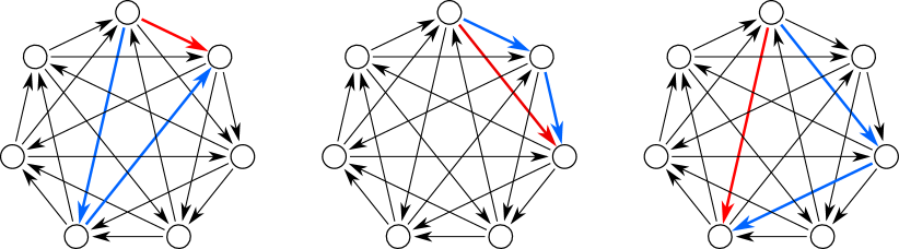
  Figure 4: Three possible cases for arcs in the color graph used in the proof of Theorem 3.15.

• If $G$ consists of a pair of vertices connected by a single arc, the coloring is given by our invariant.

This shows the statement of the theorem. ∎

For the optimality of the shown bound, we give the following example.

Example 3.16

The esp-expression

$$\begin{array}[]{lcl}X_{3}&=&((v_{1},v_{4})\cup((v_{1},v_{2})\times((v_{2},v_{4})\cup((v_{2},v_{3})\times(v_{3},v_{4})))))\times\\ &&((((v_{4},v_{6})\cup((v_{4},v_{5})\times(v_{5},v_{6})))\times(v_{6},v_{7}))\cup(v_{4},v_{7}))\end{array}$$

defines the esp-digraph on 7 vertices shown in Figure 5 and it obviously holds that $\chi_{o}(\mbox{digraph}(X_{3}))=7$. This implies that the bound of Theorem 3.15 is best possible.

Figure 5: $\mbox{Digraph}(X_{3})$ in Example 3.16.

In order to compute the oriented chromatic number of an esp-digraph $G=(V,E)$ defined by an esp-expression $X$, we recursively compute the set $F(X)$ of all triples $(H,\ell,r)$ such that $H$ is a color graph for $G$, where $\ell$ and $r$ are the colors of the source and sink, respectively, in $G$ with respect to the coloring by $H$. The number of vertex labeled, i.e., the vertices are distinguishable from each other, oriented graphs on $n$ vertices is $3^{\nicefrac{{n(n-1)}}{{2}}}$. By Theorem 3.15 and also by Corollary 3.14 we can conclude that

$$|F(X)|\leq 3^{\nicefrac{{7(7-1)}}{{2}}}\cdot 7\cdot 7\in\text{$\mathcal{O}$}(1)$$

which is independent of the size of $G$.

For two color graphs $H_{1}=(V_{1},E_{1})$ and $H_{2}=(V_{2},E_{2})$ we define $H_{1}+H_{2}=(V_{1}\cup V_{2},E_{1}\cup E_{2})$.

Lemma 3.17

1. For every $(u,v)\in E$ it holds

   $$F((u,v))=\{((\{i,j\},\{(i,j)\}),i,j)\mid 1\leq i,j\leq 7,~{}i\neq j\}.$$

2. For every two esp-expressions $X_{1}$ and $X_{2}$ we obtain $F(X_{1}\cup X_{2})$ from $F(X_{1})$ and $F(X_{2})$ as follows. For every $(H_{1},\ell_{1},r_{1})\in F(X_{1})$ and every $(H_{2},\ell_{2},r_{2})\in F(X_{2})$ such that graph $H_{1}+H_{2}$ is oriented, $\ell_{1}=\ell_{2}$, and $r_{1}=r_{2}$, we put $(H_{1}+H_{2},\ell_{1},r_{1})$ into $F(X_{1}\cup X_{2})$.

3. For every two esp-expressions $X_{1}$ and $X_{2}$ we obtain $F(X_{1}\times X_{2})$ from $F(X_{1})$ and $F(X_{2})$ as follows. For every $(H_{1},\ell_{1},r_{1})\in F(X_{1})$ and every $(H_{2},\ell_{2},r_{2})\in F(X_{2})$ such that graph $H_{1}+H_{2}$ is oriented, and $r_{1}=\ell_{2}$, we put $((V_{1}\cup V_{2},E_{1}\cup E_{2}),\ell_{1},r_{2})$ into $F(X_{1}\times X_{2})$.

Proof.

We show for each operation that the stated formulas hold.

1. Set $F((u,v))$ includes obviously all possible solutions to color the end vertices of every arc on its own with the $7$ given colors.

2. Set $F(X_{1})$ includes all possible solutions for coloring $X_{1}$, just as $F(X_{2})$ for $X_{2}$. In particular we have solutions included, that are equal but a permutation of the colors. Since the sources and sinks are each identified with each other, we only keep solutions where $\ell_{1}=\ell_{2}$ and $r_{1}=r_{2}$. In this step it is essential that we kept all possible solutions before, even if they are just permutations of the different colors. $H_{1}+H_{2}$ is oriented and has by construction at most 7 vertices. Since in $\mbox{digraph}(X_{1}\cup X_{2})$ there are no additional edges compared to $E_{1}\cup E_{2}$, every vertex can get the same color as in the individual solutions, such that all vertices are legally colored. So $(H_{1}+H_{2},\ell_{1},r_{1})$ is an possible solution to color and thus $(H_{1}+H_{2},\ell_{1},r_{1})\in F(X_{1}\cup X_{2})$.

   Let $(H,\ell,r)\in F(X_{1}\cup X_{2})$, then we can take an induced subdigraph $H_{1}$ which colors all the vertices of $\mbox{digraph}(X_{1})$ as well as $H_{2}$ which colors all the vertices of $H_{2}$. Let $\ell_{1}=\ell$ be the color of the source in $\mbox{digraph}(X_{1})$ and $r_{1}=r$ the color of the sink in $\mbox{digraph}(X_{2})$. It holds that $(H_{1},\ell_{1},r_{1})\in F(X_{1})$. The same arguments hold for $X_{2}$ such that $(H_{2},\ell_{2},r_{2})\in F(X_{2})$.

3. Set $F(X_{1})$ includes all possible solutions for coloring $X_{1}$, just as $F(X_{2})$ for $X_{2}$. In particular we have solutions included, that are equal but a permutation of the colors. Since the source and the sink are identified with each other, we only keep solutions where $r_{1}=\ell_{2}$. In this step it is essential that we kept all possible solutions before, even if they are just permutations of the different colors. $H_{1}+H_{2}$ is oriented and has by construction at most 7 vertices. In $\mbox{digraph}(X_{1}\times X_{2})$ there no additional edges compared to $E_{1}\cup E_{2}$, every vertex can get the same color as in the individual solutions, such that all vertices are legally colored. So $(H_{1}+H_{2},\ell_{1},r_{2})$ is a possible solution and thus, $(H_{1}+H_{2},\ell_{1},r_{2})\in F(X_{1}\times X_{2})$.

   Let $(H,\ell,r)\in F(X_{1}\times X_{2})$, then we can take an induced subdigraph $H_{1}$ which colors all the vertices of $\mbox{digraph}(X_{1})$ as well as $H_{2}$ which colors all the vertices of $H_{2}$. Let $\ell_{1}=\ell$ be the color of the source in $\mbox{digraph}(X_{1})$ and $r_{1}$ the color of the sink in $\mbox{digraph}(X_{2})$. It holds that $(H_{1},\ell_{1},r_{1})\in F(X_{1})$. The same arguments hold for $X_{2}$, if $\ell_{2}$ is the color of the source of $\mbox{digraph}(X_{1})$ and $r_{1}=r$ is the color of the sink of $\mbox{digraph}(X_{2})$, such that $(H_{2},\ell_{2},r_{2})\in F(X_{2})$.

This shows the statements of the lemma. ∎

The optimal solution for digraph $G$ given by an esp-expression $X$ is always included in $F(X)$ since all possible sub-solutions are maintained in the process and not only the optimal solutions. We can show this shortly by contradiction. Assumed there exists an optimal solution $(H,\ell,r)$ for $X_{1}\times X_{2}$, but $(H,\ell,r)\not\in F(X_{1}\times X_{2})$ such that $(H,\ell,r)$ was not taken into the solution. Thus, for either $X_{1}$ or $X_{2}$ (which we call $X_{i}$ in the following), the solution of coloring the vertices with color graph $H^{\prime}$, which is an induced subdigraph of $H$ and which only contains the colors we need for coloring $X_{i}$, was not part of the solution $F(X)$. But since there are all the possible solutions in $F(X)$ and not only minimal solutions, this is a contradiction to our procedure. The same holds for the parallel composition $X_{1}\cup X_{2}$. Thus, we find a minimal coloring for $G$. We know from Theorem 3.2 that the number of colors in an optimal solution is limited by 7.

Corollary 3.18

There is an oriented vertex $r$-coloring for an esp-digraph $G$ which is given by an esp-expression $X$ if and only if there is some $(H,\ell,r)\in F(X)$ such that color graph $H$ has $r$ vertices. Therefore, $\chi_{o}(G)=\min\{|V|\mid((V,E),\ell,r)\in F(X)\}$.

Theorem 3.19

Let $G$ be an esp-digraph. Then, the oriented chromatic number of $G$ can be computed in linear time.

Proof.

Let $G=(V,E)$ be an esp-digraph with $n=|V|$ vertices and $m=|E|$ edges and let $T$ be an esp-tree for $G$ with root $r$. For a vertex $u$ of $T$ we denote by $T_{u}$ the subtree rooted at $u$ and by $X_{u}$ the esp-expression defined by $T_{u}$.

For computing the oriented chromatic number for an esp-digraph $G$, we traverse esp-tree $T$ in bottom-up order. For every vertex $u$ of $T$ we can compute $F(X_{u})$ by following the rules given in Lemma 3.17. By Corollary 3.18 we can solve our problem using $F(X_{r})=F(X)$.

An esp-tree $T$ can be computed in $\text{$\mathcal{O}$}(n+m)$ time from $G$, see [Val78]. By Lemma 3.17 we obtain the following running times.

• For every vertex $(u,v)\in E$ set $F((u,v))$ is computable in $\text{$\mathcal{O}$}(1)$ time.

• For every two esp-expressions $X_{1}$ and $X_{2}$ set $F(X_{1}\cup X_{2})$ can be computed in $\text{$\mathcal{O}$}(1)$ time from $F(X_{1})$ and $F(X_{2})$.

• For every two esp-expressions $X_{1}$ and $X_{2}$ set $F(X_{1}\times X_{2})$ can be computed in $\text{$\mathcal{O}$}(1)$ time from $F(X_{1})$ and $F(X_{2})$.

Since $T$ consists of $n$ leaves and $n-1$ inner vertices, the overall running time is in $\text{$\mathcal{O}$}(n+m)$. ∎

4 Minimal Vertex Series-Parallel Digraphs

We recall the definition of minimal vertex series-parallel digraphs from [BJG18] which are based on [VTL82].

Definition 4.1 (Minimal Vertex Series-Parallel Digraphs)

The class of minimal vertex series-parallel digraphs, msp-digraphs for short, is recursively defined as follows.

1. Every digraph on a single vertex $(\{v\},\emptyset)$, denoted by $v$, is a minimal vertex series-parallel digraph.

2. If $G_{1}=(V_{1},E_{1})$ and $G_{2}=(V_{2},E_{2})$ are vertex-disjoint minimal vertex series-parallel digraphs and $O_{1}$ is the set of vertex of outdegree $0$ (set of sinks) in $G_{1}$ and $I_{2}$ is the set of vertices of indegree $0$ (set of sources) in $G_{2}$, then

   1. the parallel composition $G_{1}\cup G_{2}=(V_{1}\cup V_{2},E_{1}\cup E_{2})$ is a minimal vertex series-parallel digraph and

   2. the series composition $G_{1}\times G_{2}=(V_{1}\cup V_{2},E_{1}\cup E_{2}\cup(O_{1}\times I_{2}))$ is a minimal vertex series-parallel digraph.

An expression $X$ using the operations of Definition 4.1 is called an msp-expression and $\mbox{digraph}(X)$ the defined graph. We illustrate such an expression with the following example.

Example 4.2

The msp-expression

$$X_{4}=\left(v_{1}\times\left(\left(v_{2}\times\left(v_{3}\times v_{4}\right)\right)\cup v_{5}\right)\right)\times v_{6}$$

defines the msp-digraph shown in Figure 6.

Figure 6: $\mbox{Digraph}(X_{4})$ in Example 4.2.

Several classes of digraphs are included in the set of all msp-digraphs.

Example 4.3

1. Every oriented bipartite graph $\overrightarrow{K_{n,m}}$ is an msp-digraph by the following msp-expression.

   $$X_{K_{n,m}}=(v_{1}\cup\ldots\cup v_{n})\times(w_{1}\cup\ldots\cup w_{m})$$

2. Every in- and out-rooted tree $T$ is an msp-digraph. An msp-expression $X$ can be obtained by inserting the vertices of $T$ into $X$ using a bottom-up order. We denote by $X_{v_{i}}$ the msp-expression for the subtree of $T$ rooted at $v_{i}$. For every leaf $v_{i}$ of $T$ we obviously have the msp-expression $X_{v_{i}}=v_{i}$. For every inner vertex $v_{i}$ with successors $v_{j_{1}},\ldots,v_{j_{i}}$ in $T$ the expressions $X_{v_{j_{1}}},\ldots,X_{v_{j_{i}}}$ are first combined by parallel compositions to sub-expression $X^{\prime}_{v_{i}}$ and afterwards $v_{i}$ is combined with $X^{\prime}_{v_{i}}$ using a series composition to obtain sub-expression $X_{v_{i}}$.

For every msp-digraph we can define a tree structure, denoted as msp-tree. The vertices of the graph are represented by the leaves of the msp-tree. Meanwhile, the inner nodes of the msp-tree correspond to the operations which are applied on the sub-expressions defined by the subtrees. For a vertex $u$ of msp-tree $T$ we denote by $T(u)$ the subtree which is rooted at $u$ and by $X(u)$ the sub-expression defined by $T(u)$.

For every msp-digraph we can construct a msp-tree in linear time, see [VTL82].

Further, there is a close relation between esp-digraphs and msp-digraphs, which the following Lemma shows.

Lemma 4.4 ([VTL82])

An acyclic multidigraph $G$ with a single source and a single sink is an esp-digraph if and only if its line digraph $LD(G)$ is a msp-digraph.

Example 4.5

The msp-digraph $\mbox{digraph}(X_{4})$, which is defined in Example 4.2 and shown in Figure 6, defines the line digraph of esp-digraph $\mbox{digraph}(X_{1})$ defined in Example 3.5, see Figure 1.

Next we compare the classes of msp-digraphs and esp-digraphs.

Remark 4.6

The classes of msp-digraphs and esp-digraphs are incomparable in terms of set inclusion. Example 3.6(2.) gives a class of esp-digraphs which are not msp-digraphs and Example 4.3(1.). gives a class of msp-digraphs which are not esp-digraphs.

Remark 4.7

In contrast to Remark 3.9 on esp-digraphs, there are classes of msp-digraphs which are not orientations of a series-parallel graph. This can be shown by Example 4.3(1.). The underlying undirected graphs of oriented bipartite graphs $\overrightarrow{K_{n,m}}$ have unbounded tree-width while the set of series-parallel graphs has tree-width at most 2 [Bod98].

4.1 Oriented Vertex-Colorings of Minimal Vertex Series-Parallel Digraphs

Using the recursive structure of msp-digraphs we could show the following bound on their oriented chromatic number.

Proposition 4.8 ([GKL20, GKL21b])

Let $G$ be an msp-digraph. Then, it holds that $\chi_{o}(G)\leq 7$.

Remark 4.9

We can also bound the oriented chromatic number of a msp-digraph $G$ using the corresponding root digraph $G^{\prime}$ which is an esp-digraph by Lemma 4.4.

$$\begin{array}[]{lclll}\chi_{o}(G)&=&\chi_{o}(LD(G^{\prime}))&\text{Lemma }\ref{le-vtl}\\ &=&\chi^{\prime}_{o}(G^{\prime})&\text{Observation }\ref{obs-nu-in}\\ &\leq&7&\text{Corollary }\ref{cor-77}\end{array}$$

For the optimality of the shown bound, we recall from [GKL20] the following example.

Example 4.10 ([GKL20])

We consider the msp-expression

$$\begin{array}[]{lcl}X_{5}&=&v_{1}\times(v_{2}\cup v_{3}\times(v_{4}\cup v_{5}\times v_{6}))\times(v_{7}\cup(v_{8}\cup v_{9}\times v_{10})\times(v_{11}\cup v_{12}\times v_{13}))\times\\ &&(v_{14}\cup(v_{15}\cup(v_{16}\cup v_{17}\times v_{18})\times(v_{19}\cup v_{20}\times v_{21}))\times\\ &&(v_{22}\cup(v_{23}\cup v_{24}\times v_{25})\times v_{26}))\times v_{27}\end{array}$$

Since by [GKL20] it holds that $\chi_{o}(\mbox{digraph}(X_{5}))=7$ the bound of Proposition 4.8 is best possible.

Using the upper bound on the oriented chromatic number and the recursive structure of msp-digraphs we achieve a linear time solution for computing the oriented chromatic number of msp-digraphs.

Theorem 4.11 ([GKL20, GKL21b])

Let $G$ be a msp-digraph. Then, the oriented chromatic number of $G$ can be computed in linear time.

4.2 Oriented Arc-Colorings of Minimal Vertex Series-Parallel Digraphs

By Proposition 4.8 and Observation 2.7 we know the following bound on the oriented chromatic index of msp-digraphs.

Corollary 4.12

Let $G$ be an msp-digraph. Then, it holds that $\chi^{\prime}_{o}(G)\leq 7$.

For the optimality of the shown bound, we next give an example.

Example 4.13

We recursively define msp-expressions $Y_{i}$ as follows. $Y_{0}$ defines a single vertex graph and for $i\geq 1$ we define

$$Y_{i}=(Y_{0}\cup Y_{i-1}\times Y_{i-1})$$

in order to define

$$X_{6}=Y_{0}\times Y_{0}\times Y_{6}\times Y_{0}\times Y_{0}.$$

$\mbox{Digraph}(X_{6})$ has 131 vertices and satisfies $\chi^{\prime}_{o}(\mbox{digraph}(X_{6}))=7$, which was found by a binary integer program (Remark 2.8) using Gorubipy. This implies that the bound of Corollary 4.12 is best possible.

In order to compute the oriented chromatic index of an msp-digraph $G=(V,E)$ defined by an msp-expression $X$, we apply Observation 2.6 which allows us to compute the oriented chromatic number of $LD(G)$. This is done by computing triples $(H,\mathcal{L},\mathcal{R})$, which are defined as follows. Here $H=(V_{H},E_{H})$ is a color graph of $LD(G)$ with $V_{H}\subseteq\{1,\dots,7\}$. At first we do not care whether the color graphs are oriented or even contain loops. At the end we then check which is the color graph with the fewest vertices that is oriented.

The color graph of $LD(G)$ for the parallel composition $G=G_{1}\cup G_{2}$ can easily be obtained from the color graphs $H_{1}=(V_{1},E_{1})$ of $LD(G_{1})$ and $H_{2}=(V_{2},E_{2})$ of $LD(G_{2})$ by $H_{1}+H_{2}:=(V_{1}\cup V_{2},E_{1}\cup E_{2})$.

Example 4.14

In Figure 7 the construction of a color graph of $LD(G)$ for $G=G_{1}\cup G_{2}$ is illustrated.

Figure 7: $H_{1}$ is a color graph of $LD(G_{1})$ and $H_{2}$ is a color graph of $LD(G_{2})$, so $H_{1}+H_{2}$ is a color graph of $LD(G_{1}\cup G_{2})$.

The color graph of $LD(G)$ for the series composition $G=G_{1}\times G_{2}$ obviously has new vertices which correspond to the new inserted edges by the series composition in $G$.

Example 4.15

We consider the series composition $G=G_{1}\times G_{2}$ in Figure 8. If $H_{1}$ is the color graph of the coloring of $LD(G_{1})$ and $H_{2}$ is the color graph of the coloring of $LD(G_{2})$, then we get several possible color graphs depending on how $x_{1}$, $x_{2}$, $y_{1}$ and $y_{2}$ are colored.

The color graphs are of the form $H_{1}+H_{2}$ with additional vertices for the edges $(1,x_{i})$, $(2,x_{i})$, $(x_{i},3)$, $(1,y_{i})$, $(2,y_{i})$ and $(y_{i},4)$ with $i=1$ or $2$.

So in order to determine all possible color graphs of $G_{1}\times G_{2}$, we have to know that $G_{1}$ has two sinks with leading edges colored with 1 and 2 and $G_{2}$ has one source with one leading edge colored with 3 and one source with one leading edge colored with 4.

As a first simplification, we can assume, without loss of generality, that $x_{1}=x_{2}$ and $y_{1}=y_{2}$. This applies because every oriented coloring with $x_{1}\neq x_{2}$ also remains oriented when $x_{1}=x_{2}$. So we do not need to know that $G_{1}$ has two sinks, which have incoming edges colored with 1 and 2, it is enough to know that $G_{1}$ has at least one such sink.

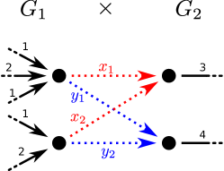
Figure 8: Example of a series composition $G=G_{1}\times G_{2}$

The example shows that we need the colors of the incoming edges of sinks and the colors of the outgoing edges of sources in $G$. In order to store these informations let $\mathcal{L}\subseteq\mathcal{P}(\{1,\dots,7\})$ be the set of the sets $L$ such that there is a source $\ell$ in $G$, such that $L$ is the set of outgoing edge colors in $\ell$ and $\mathcal{R}\subseteq\mathcal{P}(\{1,\dots,7\})$ be the set of the sets $R$ such that there is a sink $r$ in $G$, such that $R$ is the set of outgoing edge colors in $r$.

Assume we know the triples $((V_{1},E_{1}),\mathcal{L}_{1},\mathcal{R}_{1})$ for $G_{1}$ and the triples $((V_{2},E_{2}),\mathcal{L}_{2},\mathcal{R}_{2})$ for $G_{2}$. For every $R\in\mathcal{R}_{1}$ and every $L\in\mathcal{L}_{2}$ we define a new vertex $u_{R,L}$ in $H$, which represents the color of all new edges that go from a sink $r$ of $G_{1}$, whose incoming edge colors are $R$, to a source $\ell$ of $G_{2}$, whose outgoing edge colors are $L$.

Example 4.16

In Figure 8 the color of the red edges would be $u_{\{1,2\},\{3\}}$ and the color of the blue edges $u_{\{1,2\},\{4\}}$, representing two new vertices in the color graph $H$.

For a color graph $H$ of $LD(G_{1}\times G_{2})$ we have the edges of $H_{1}$ and $H_{2}$ and additionally the edges $\bigcup_{R_{i}\in\mathcal{R}_{1}}(R_{i}\times\{u_{R_{i},L_{j}}\mid L_{j}\in\mathcal{L}_{2}\})$ and $\bigcup_{L_{j}\in\mathcal{L}_{2}}(\{u_{R_{i},L_{j}}\mid R_{i}\in\mathcal{R}_{1}\}\times L_{j})$.

Example 4.17

In Figure 8 the additional edges in color graph $H$ are $\{1,2\}\times\{u_{\{1,2\},\{3\}},u_{\{1,2\},\{4\}}\}$ and $\{u_{\{1,2\},\{3\}}\}\times\{3\}\cup\{u_{\{1,2\},\{4\}}\}\times\{4\}$.

To obtain the new set $\mathcal{L}$ for $\mbox{digraph}(X_{1}\times X_{2})$ we have to distinguish between the following two cases. If $\emptyset\not\in\mathcal{L}_{1}$, i.e. $\mbox{digraph}(X_{1})$ has no isolated vertices, then $\mathcal{L}=\mathcal{L}_{1}$ applies. If $\emptyset\in\mathcal{L}_{1}$, then $\mathcal{L}=(\mathcal{L}_{1}-\{\emptyset\})\cup\{\{u_{\emptyset,L_{j}}\mid L_{j}\in\mathcal{L}_{2}\}\}$. The same can be concluded for the new set $\mathcal{R}$ for $\mbox{digraph}(X_{1}\times X_{2})$. Thus, $\mathcal{R}$ and $\mathcal{L}$ can easily be constructed together with the color graph.

We store all these triples $(H,\mathcal{L},\mathcal{R})$ in $F(X)$. In order to bound the size of $F(X)$ we recall that the number of vertex labeled, i.e., the vertices are distinguishable from each other, oriented graphs on $n$ vertices is $3^{\nicefrac{{n(n-1)}}{{2}}}$. By Corollary 4.12 we can conclude that

$$|F(X)|\leq 3^{\nicefrac{{7(7-1)}}{{2}}}\cdot 2^{2^{7}}\cdot 2^{2^{7}}\in\text{$\mathcal{O}$}(1)$$

which is independent of the size of $G$.

Lemma 4.18

1. For every $v\in V$ it holds that

   $$F(v)=\{((\emptyset,\emptyset),\{\emptyset\},\{\emptyset\})\}.$$

2. Let $X=X_{1}\cup X_{2}$, then it holds that

   $$F(X)=\left\{(H_{1}+H_{2},\mathcal{L}_{1}\cup\mathcal{L}_{2},\mathcal{R}_{1}\cup\mathcal{R}_{2})\ \middle|\begin{array}[]{l}(H_{1},\mathcal{L}_{1},\mathcal{R}_{1})\in F(X_{1}),\\ (H_{2},\mathcal{L}_{2},\mathcal{R}_{2})\in F(X_{2})\end{array}\right\}.$$

3. Let $X=X_{1}\times X_{2}$, then it holds that

   $$F(X)=\left\{(H,\mathcal{L},\mathcal{R})\ \middle|\begin{array}[]{l}((V_{1},E_{1}),\mathcal{L}_{1},\mathcal{R}_{1})\in F(X_{1}),\\ ((V_{2},E_{2}),\mathcal{L}_{2},\mathcal{R}_{2})\in F(X_{2}),\\ u_{R_{i},L_{j}}\in\{1,\dots,7\}\ \forall R_{i}\in\mathcal{R}_{1},L_{j}\in\mathcal{L}_{2},\text{ where}\\ U_{1,R_{i}}=\{u_{R_{i},L_{j}}\mid L_{j}\in\mathcal{L}_{2}\},\\ U_{2,L_{j}}=\{u_{R_{i},L_{j}}\mid R_{i}\in\mathcal{R}_{1}\},\\ U=\{u_{R_{i},L_{j}}\mid R_{i}\in\mathcal{R}_{1},L_{j}\in\mathcal{R}_{2}\},\\ \mathcal{L}=\begin{cases}\mathcal{L}_{1}&\text{if }\emptyset\notin\mathcal{L}_{1}\\ (\mathcal{L}_{1}-\{\emptyset\})\cup\{U_{1,\emptyset}\}&\text{if }\emptyset\in\mathcal{L}_{1}\end{cases},\\ \mathcal{R}=\begin{cases}\mathcal{R}_{2}&\text{if }\emptyset\notin\mathcal{R}_{2}\\ (\mathcal{R}_{2}-\{\emptyset\})\cup\{U_{2,\emptyset}\}&\text{if }\emptyset\in\mathcal{R}_{2}\end{cases},\\ H=(V,E),\\ V=V_{1}\cup V_{2}\cup U,\\ E=E_{1}\cup E_{2}\underset{R_{i}\in\mathcal{R}_{1}}{\bigcup}(R_{i}\times U_{1,R_{i}})\underset{L_{j}\in\mathcal{L}_{2}}{\bigcup}(U_{2,L_{j}}\times L_{j})\end{array}\right\}.$$

Corollary 4.19

There is an oriented edge $r$-coloring for an msp-digraph $G$ which is given by an msp-expression $X$ if and only if there is some $(H,\mathcal{L},\mathcal{R})\in F(X)$ such that color graph $H$ has $r$ vertices and is oriented. Therefore, $\chi_{o}^{\prime}(G)=\min\{|V_{H}|\mid((V_{H},E_{H}),\mathcal{L},\mathcal{R})\in F(X)\text{ and }(V_{H},E_{H})\text{ is oriented}\}$.

Theorem 4.20

Let $G$ be a msp-digraph. Then, the oriented chromatic index of $G$ can be computed in linear time.

Proof.

Let $G=(V,E)$ be an msp-digraph with $n=|V|$ vertices and $m=|E|$ edges and let $T$ be an msp-tree for $G$ with root $r$. For a vertex $u$ of $T$ we denote by $T_{u}$ the subtree rooted at $u$ and by $X_{u}$ the esp-expression defined by $T_{u}$.

For computing the oriented chromatic index for an msp-digraph $G$, we traverse msp-tree $T$ in bottom-up order. For every vertex $u$ of $T$ we can compute $F(X_{u})$ by following the rules given in Lemma 4.18. By Corollary 4.19 we can solve our problem using $F(X_{r})=F(X)$.

An msp-tree $T$ can be computed in $\text{$\mathcal{O}$}(n+m)$ time from $G$, see [VTL82]. By Lemma 4.18 we obtain the following running times.

• For every vertex $v\in V$ set $F(v)$ is computable in $\text{$\mathcal{O}$}(1)$ time.

• For every two msp-expressions $X_{1}$ and $X_{2}$ set $F(X_{1}\cup X_{2})$ and set $F(X_{1}\times X_{2})$ can be computed in $\text{$\mathcal{O}$}(1)$ time from $F(X_{1})$ and $F(X_{2})$. This is true since there are only a constant number of color graphs with nodes from $\{1,\ldots,7\}$, just as there are only a limited number of different $\mathcal{L}$ and $\mathcal{R}$ and so the input size is constant.

Since $T$ consists of $n$ leaves and $n-1$ inner vertices, the overall running time is in $\text{$\mathcal{O}$}(n+m)$. ∎

5 Conclusions and outlook

In this paper we showed tight upper bounds for the oriented chromatic number and the oriented chromatic index of edge series-parallel digraphs and minimal series-parallel digraphs. Furthermore, we introduced linear time solutions for computing the oriented chromatic number of edge series-parallel digraphs and the oriented chromatic index of minimal series-parallel digraphs.

The existence of graph classes of arbitrary large vertex degree but bounded oriented chromatic index, such as msp-digraph and esp-digraphs, implies that Vizings Theorem [Viz64] can not be carried over to the oriented chromatic index.

In our future work we want to analyze the existence of polynomial time algorithms for computing the oriented chromatic index and oriented chromatic number of orientations of series-parallel graphs efficiently which would lead to generalizations of Theorem 3.13 and Theorem 3.19.

Furthermore, it remains to extend the results for OCN and OCI to graphs of bounded directed clique-width. As a starting point we considered the parameterized complexity of $\text{OCN}_{r}$ parameterized by directed clique-width in [GKL21a].

References

- [BJG09] J. Bang-Jensen and G. Gutin. Digraphs. Theory, Algorithms and Applications. Springer-Verlag, Berlin, 2009.
- [BJG18] J. Bang-Jensen and G. Gutin, editors. Classes of Directed Graphs. Springer-Verlag, Berlin, 2018.
- [BLS99] A. Brandstädt, V.B. Le, and J.P. Spinrad. Graph Classes: A Survey. SIAM Monographs on Discrete Mathematics and Applications. SIAM, Philadelphia, 1999.
- [Bod98] H.L. Bodlaender. A partial -arboretum of graphs with bounded treewidth. Theoretical Computer Science, 209:1–45, 1998.
- [CD06] J.-F. Culus and M. Demange. Oriented coloring: Complexity and approximation. In Proceedings of the Conference on Current Trends in Theory and Practice of Computer Science (SOFSEM), volume 3831 of LNCS, pages 226–236. Springer-Verlag, 2006.
- [CLSB81] D.G. Corneil, H. Lerchs, and L. Stewart-Burlingham. Complement reducible graphs. Discrete Applied Mathematics, 3:163–174, 1981.
- [Cou94] B. Courcelle. The monadic second-order logic of graphs VI: On several representations of graphs by relational structures. Discrete Applied Mathematics, 54:117–149, 1994.
- [Dai80] D.P. Dailey. Uniqueness of colorability and colorability of planar 4-regular graphs are NP-complete. Discrete Mathematics, 30(3):289–293, 1980.
- [DS14] J. Dybizbański and A. Szepietowski. The oriented chromatic number of Halin graphs. Information Processing Letters, 114(1-2):45–49, 2014.
- [Epp92] D. Eppstein. Parallel recognition of series-parallel graphs. Information and Computation, 98(1):41–55, 1992.
- [GKL20] F. Gurski, D. Komander, and M. Lindemann. Oriented coloring of msp-digraphs and oriented co-graphs. In Proceedings of the International Conference on Combinatorial Optimization and Applications (COCOA), volume 12577 of LNCS, pages 743–758. Springer-Verlag, 2020.
- [GKL21a] F. Gurski, D. Komander, and M. Lindemann. Efficient computation of the oriented chromatic number of recursively defined digraphs. Theoretical Computer Science, 890:16–35, 2021.
- [GKL21b] F. Gurski, D. Komander, and M. Lindemann. Homomorphisms to digraphs with large girth and oriented colorings of minimal series-parallel digraphs. In Proceedings of the International Workshop on Algorithms and Computation (WALCOM), volume 12635 of LNCS, pages 182–194. Springer-Verlag, 2021.
- [GKR19] F. Gurski, D. Komander, and C. Rehs. Oriented coloring on recursively defined digraphs. Algorithms, 12(4):87, 2019.
- [GO15] G. Guegan and P. Ochem. Complexity dichotomy for oriented homomorphism of planar graphs with large girth. Theoretical Computer Science, 596:142–148, 2015.
- [Gur14] F. Gurski. Efficient binary linear programming formulations for boolean functions. Statistics, Optimization and Information Computing, 2(4):274–279, 2014.
- [HN60] F. Harary and R.Z. Norman. Some properties of line digraphs. Rend. Circ. Mat. Palermo, 9(2):161–168, 1960.
- [HY87] X. He and Y. Yesha. Parallel recognition and decomposition of two terminal series parallel graphs. Information and Computation, 75:15–38, 1987.
- [KM04] W.F. Klostermeyer and G. MacGillivray. Homomorphisms and oriented colorings of equivalence classes of oriented graphs. Discrete Mathematics, 274:161–172, 2004.
- [LGK21] M. Lindemann, F. Gurski, and D. Komander. Oriented vertex and arc coloring of edge series-parallel digraphs. In Operations Research Proceedings (OR 2021), Selected Papers. Springer-Verlag, 2021. to appear.
- [Mar13] T.H. Marshall. Homomorphism bounds for oriented planar graphs of given minimum girth. Graphs and Combin., 29:1489–1499, 2013.
- [Mar15] T.H. Marshall. On oriented graphs with certain extension properties. Ars Combinatoria, 120:223–236, 2015.
- [OP14] P. Ochem and A. Pinlou. Oriented coloring of triangle-free planar graphs and 2-outerplanar graphs. Graphs and Combin., 30:439–453, 2014.
- [OPS08] P. Ochem, A. Pinlou, and E. Sopena. On the oriented chromatic index of oriented graphs. Journal of Graph Theory, 57(4):313–332, 2008.
- [PS06] A. Pinlou and E. Sopena. Oriented vertex and arc coloring of outerplanar graphs. Information Processing Letters, 100:97–104, 2006.
- [Sey90] P.D. Seymour. Colouring series-parallel graphs. Combinatorica, 10(4):379–392, 1990.
- [Sop97] E. Sopena. The chromatic number of oriented graphs. Journal of Graph Theory, 25:191–205, 1997.
- [Sop16] E. Sopena. Homomorphisms and colourings of oriented graphs: An updated survey. Discrete Mathematics, 339:1993–2005, 2016.
- [Val78] J. Valdes. Parsing flowcharts and series-parallel graphs. Technical Report STAN-CS-78-682, Computer Science Department, Stanford University, Stanford, California, 1978.
- [Viz64] V.G. Vizing. On an estimate of the chromatic class of a p-graph. Metody Diskret. Analiz., 3:9–17, 1964.
- [VTL82] J. Valdes, R.E. Tarjan, and E.L. Lawler. The recognition of series-parallel digraphs. SIAM Journal on Computing, 11:298–313, 1982.