A Less Uncertain Sampling-Based Method
of Batch Bayesian Optimization

Abstract

This paper presents a method called sampling-computation-optimization (SCO) to design batch Bayesian optimization. SCO does not construct new high-dimensional acquisition functions but samples from the existing one-site acquisition function to obtain several candidate samples. To reduce the uncertainty of the sampling, the general discrepancy is computed to compare these samples. Finally, the genetic algorithm and switch algorithm are used to optimize the design. Several strategies are used to reduce the computational burden in the SCO. From the numerical results, the SCO designs were less uncertain than those of other sampling-based methods. As for application in batch Bayesian optimization, SCO can find a better solution when compared with other batch methods in the same dimension and batch size. In addition, it is also flexible and can be adapted to different one-site methods. Finally, a complex experimental case is given to illustrate the application value and scenario of SCO method.

Keywords: Batch sequential design; Rejection sampling; Sampling-importance-resampling; General discrepancy; Global optimization

1 Introduction

Bayesian optimization is important in the engineering optimization field. The general idea of Bayesian optimization is as follows:

1. Build or update the surrogate model $\hat{f}_{\rm exp}$ based on the database $Y_{\rm data}=f_{\rm exp}(X_{\rm data})$; $\hat{f}_{\rm exp}$ usually provides the prediction or description of the experiment response and is easy to solve;

2. Construct the acquisition function $\phi(\bm{x})=\phi(\bm{x}|X_{\rm data},Y_{\rm data},\hat{f}_{\rm exp})$ to evaluate the value of further experiments on $\Omega$ according to the model and experiment purposes;

3. Choose the most valuable sites $\bm{x}^{*}=\arg\max\phi(\bm{x})$ by some auxiliary optimization to arrange the sequential experiments;

4. Conduct the sequential experiments, and update the database.

The acquisition function $\phi$ is usually the function of one site. The classic Bayesian efficient global optimization (EGO) method (Jones et al.,, 1998) uses a proposed expected improvement (EI), based on a Gaussian process model as an acquisition function, which is efficient and widely used. According to (iii), the sequential experiments only include one site in each experiment period. However, this is very time-consuming, especially when there are many parallel experimental resources. In order to make better use of these resources, the experimenter needs to identify multiple sequential experimental sites for each period.

One way to implement this is to choose several sub-optimal sites under $\phi$, but these sub-optimal sites may converge to a cluster, which make the experiment inefficient. The other way is to construct a multi-point acquisition function $\phi(\bm{x}_{1},\dots,\bm{x}_{n})$, such as $q$-EI (Ginsbourger et al.,, 2008, 2010). However, a multi-point acquisition function is usually highly dimensional, which make it difficult to compute and optimize.

To solve the above problems, sampling technique is used to implement batch Bayesian optimization. Cai et al., (2017) and Wang et al., (2004) use the mode-pursuing sampling method (Fu and Wang,, 2002) to obtain the sequential design. Ning et al., (2020) use the sampling-importance-resampling method to accelerate EGO. However, sampling methods are arbitrary and uncertain, which is not appropriate in an expensive experiment.

This article presents a method called sampling-computation-optimization (SCO) to design the sequential experiments of batch Bayesian optimization. SCO does not construct new high-dimensional acquisition functions; instead it samples from the existing one-site acquisition function to obtain several candidate samples. Some calculations and optimizations then proceed to obtain the sequential design. The rest of this paper is organized as follows. Section 2 introduces two important sampling methods and the general discrepancy concept. The details of the SCO method are described in Section 3. Some numerical analyses and comparisons are presented in Section 4.

2 Preliminary

2.1 Rejection sampling and sampling-importance-resampling

Rejection sampling (RS) and sampling-importance-resampling (SIR) are two widely used sampling methods. We introduce the two methods briefly, for more information, see Bishop, (2006).

Suppose we would like to sample from a target density $f(\cdot)\propto\phi(\cdot)$ on $\Omega$, which is hard to sample directly but easy to compute. The main steps of RS are as follows:

1. : Choose a proposal distribution with density $g(\cdot)$, which is easy to sample.

2. : Find a constant $M$ that is large enough to ensure $\phi(\bm{x})\leq Mg(\bm{x}),\ \forall\bm{x}\in\Omega$.

3. : Generate $\bm{u}_{i}\sim g(\cdot)$ and $v_{i}\sim{\rm U}(0,1)$.

4. : If $\phi(\bm{u}_{i})<Mg(\bm{u}_{i})v_{i}$, then accept $\bm{u}_{i}$ as a sample $\bm{x}_{j}$. Otherwise, reject $\bm{u}_{i}$.

As indicated by Bishop, (2006), $\bm{x}_{j}\sim f(\cdot)$, and the probability to accept $\bm{u}_{i}$ is inversely proportional to $M$. Generally, one needs to choose a smallest $M$ to ensure $\phi(\bm{x})\leq Mg(\bm{x}),\ \forall\bm{x}\in\Omega$.

Sometimes, a suitable $M$ is difficult to find, or the reject rate is too high. We then need to turn to SIR. The main steps of SIR are as follows:

1. : Choose a proposal distribution with density $g(\cdot)$, which is easy to sample.

2. : Generate $U=\{\bm{u}_{1},\dots,\bm{u}_{N}\},\ \bm{u}_{i}\sim g(\cdot)$.

3. : Calculate the weights $w_{i}=\frac{\phi(\bm{u}_{i})/g(\bm{u}_{i})}{\sum_{i=1}^{N}\phi(\bm{u}_{i})/g(\bm{u}_{i})}$.

4. : Resample $\bm{x}_{j}$ from $U$ with the probability $(w_{1},\dots,w_{N})$.

Bishop, (2006) indicated that $\bm{x}_{j}\sim f(\cdot)$ when $N\rightarrow\infty$, which means SIR needs a large amount of pre-samples.

Both RS and SIR first need to sample $\bm{u}_{i}$ from the proposal distribution. For convenience, we call this process pre-sampling and refer to U as a pre-sample set. The two sampling methods are respectively suitable for two situations of the algorithm in this paper, and we will introduce their application in Section 3.

2.2 General Discrepancy

There are many interpretations of the discrepancy (Li et al.,, 2020). In this paper, we refer to the interpretation in Section 2.4 of Fang et al., (2018). We will begin with some basic notation.

Let $\Omega$ represent the experimental domain, and we only discuss the case when $\Omega=[0,1]^{d}$. The design is taken as a set $X=\{\bm{x}_{1},\bm{x}_{2},\dots,\bm{x}_{n}\}$ on $\Omega$. $K(\cdot,\cdot):\Omega\times\Omega\rightarrow\mathcal{R}$ is a symmetric and positive semi-definite kernel function. $F$ is a distribution function in

$$\mathcal{K}=\left\{F\left|\int_{\Omega\times\Omega}K(\bm{u},\bm{v})\mathrm{d}F(\bm{u})\mathrm{d}F(\bm{v})<\infty\right.\right\}.$$

Define the inner product of two arbitrary functions $F,G\in\mathcal{K}$ as

$$\left<F,G\right>_{K}=\int_{\Omega\times\Omega}K(\bm{u},\bm{v})\mathrm{d}F(\bm{u})\mathrm{d}G(\bm{v}).$$

The general discrepancy of the design $X$ with respect to the target distribution $F$ using the kernel $K$ is then defined as

$$D^{2}(X,F,K)\triangleq ||F_{X}-F||_{K}^{2}=\left<F_{X}-F,F_{X}-F\right>_{K}$$

$$= \int_{\Omega\times\Omega}K(\bm{u},\bm{v})\mathrm{d}(F-F_{X})(\bm{u})\mathrm{d}(F-F_{X})(\bm{v})$$

$$= \int_{\Omega\times\Omega}K(\bm{u},\bm{v})\mathrm{d}F(\bm{u})\mathrm{d}F(\bm{v})$$

$$-\frac{2}{n}\sum_{i=1}^{n}\int_{\Omega}K(\bm{u},\bm{x}_{i})\mathrm{d}F(\bm{u})+\frac{1}{n^{2}}\sum_{i,j=1}^{n}K(\bm{x}_{j},\bm{x}_{i}).$$ (2.1)

This can be taken as the distance between the target distribution $F$ and the empirical distribution of $X$. A low discrepancy means $F_{X}$ and $F$ are close in some sense, so we prefer a design with low discrepancy to better represent the target distribution.

The kernel function $K$ corresponds to an inner product of the Hilbert space. By taking different functions, we can define different kinds of discrepancy, such as the widely used centered discrepancy (CD), wrapped discrepancy (WD), or mixed discrepancy (MD). In this article, we use the kernel function of the WD (Fang et al.,, 2018):

$$K(\bm{u},\bm{v})=\prod_{i=1}^{d}\left[\frac{3}{2}-|u_{i}-v_{i}|+(u_{i}-v_{i})^{2}\right].$$ (2.2)

Because $F$ is arbitrary, the high-dimension integral in equation (2.2) is difficult to compute; we use the Monte Carlo method to estimate $D^{2}(X,F,K)$. Rewrite equation (2.2) as

$$D^{2}(X,F,K)= \int_{\Omega\times\Omega}K(\bm{u},\bm{v})\cdot f(\bm{u})\cdot f(\bm{v})\mathrm{d}\bm{u}\mathrm{d}\bm{v}$$

$$-\frac{2}{n}\sum_{i=1}^{n}\int_{\Omega}K(\bm{u},\bm{x}_{i})\cdot f(\bm{u})\mathrm{d}\bm{u}+\frac{1}{n^{2}}\sum_{i,j=1}^{n}K(\bm{x}_{j},\bm{x}_{i}).$$ (2.3)

We then get an estimation of $D^{2}(X,F,K)$ as

$$\hat{D}^{2}(X,F,K)= \frac{1}{N^{2}}\sum_{i,j=1}^{N}K(\bm{u}_{j},\bm{u}_{i})\cdot f(\bm{u}_{j})\cdot f(\bm{u}_{i})$$

$$-\frac{2}{nN}\sum_{i=1}^{n}\sum_{j=1}^{N}K(\bm{u}_{j},\bm{x}_{i})\cdot f(\bm{u}_{j})+\frac{1}{n^{2}}\sum_{i,j=1}^{n}K(\bm{x}_{j},\bm{x}_{i}),$$ (2.4)

where $\bm{u}_{i}\sim{\rm U}(\Omega),i=1,2,\dots,N$.

3 Method for batch Bayesian optimization

In this paper, we propose a method to implement batch Bayesian optimization. The new method is based on a one-site acquisition function, and its main idea is to exchange (iii) in Section 1 with a revised (iii’) as follows:

1. Take the acquisition function $\phi(\bm{x})$ as the density of a distribution $F$ and construct a sequential design $X^{*}$ to fit $F$ best;

For convenience, note $D^{2}(X,\phi,K)\triangleq D^{2}(X,F,K)$, where $F$ is induced by density $f\propto\phi$. In addition, we use $D^{2}(X,\phi,K)$ to measure the fitness described above in (iii’). If $F\sim{\rm U}(\Omega)$, this kind of sequential design is also called a uniform design. The methods for constructing uniform design are various and efficient, such as number theorem methods (Niederreiter,, 1992; Fang and Wang,, 1994; Fang et al.,, 1994), algorithmic optimization methods (Fang et al.,, 2000; Zhou et al.,, 2012; Zhou and Fang,, 2013; Chen et al.,, 2014), and hybrid methods (Zhou et al.,, 2013).

However, when F is arbitrary, it becomes complicated. The first difficulty is that number theorem methods are not suitable when $F$ is not uniform. The second is $D^{2}(X,F,K)$ has no analytic form when $F$ is arbitrary. Calculating $D^{2}(X,F,K)$ is already difficult, let alone optimizing it. As a result, the construction has to make a trade-off between optimality and feasibility, aiming to construct a design with relatively low discrepancy in an acceptable time.

In this section, we first used the sampling method to generate several candidate samples. To avoid the arbitrariness of sampling method, general discrepancy is calculated to compare candidate designs. Ultimately, the sequential design is determined through optimization. We call this method sampling-computation-optimization (SCO). Next, the details of SCO are described step-by-step.

3.1 Sampling

At the beginning, we use RS to obtain samples. The proposal distribution $g(\cdot)$ is chosen as ${\rm U}(\Omega)$ for convenience. In this way, the pre-sample set $U$ can be used in calculation, and we will explain this next. As a requirement of RS, $M$ should be large enough to ensure $\phi(\bm{x})\leq Mg(\bm{x})=M$, we need to optimize $\phi(\bm{x})$ to determine the minimum of $M$. The advantage in doing this is so that we can find the optimal $\bm{x}^{*}$ and take it as the first site of $X$; we then only sample $n-1$ points to form the candidate design. In this way, the batch Bayesian optimization can be compatible with the one-site Bayesian optimization. As mentioned previously, the probability of accepting samples in RS is inversely proportional to $M$.

Considering the rejection rate, there are two drawbacks as follows. First, when $\phi$ is relatively flat, the rejection rate is too low, and the size of $U$ is too small. Because $U$ will be used in the calculation, this will affect the accuracy of the next stage. Second, when $\phi$ is steep, the rejection rate is too high, and the sampling efficiency will be too low, resulting in a large amount of calculation. These two situations are common at the beginning and end of the EGO algorithm respectively, for example, see Figure 1. We then improve the sampling process to suit the above situations.

(a) flat at the beginning

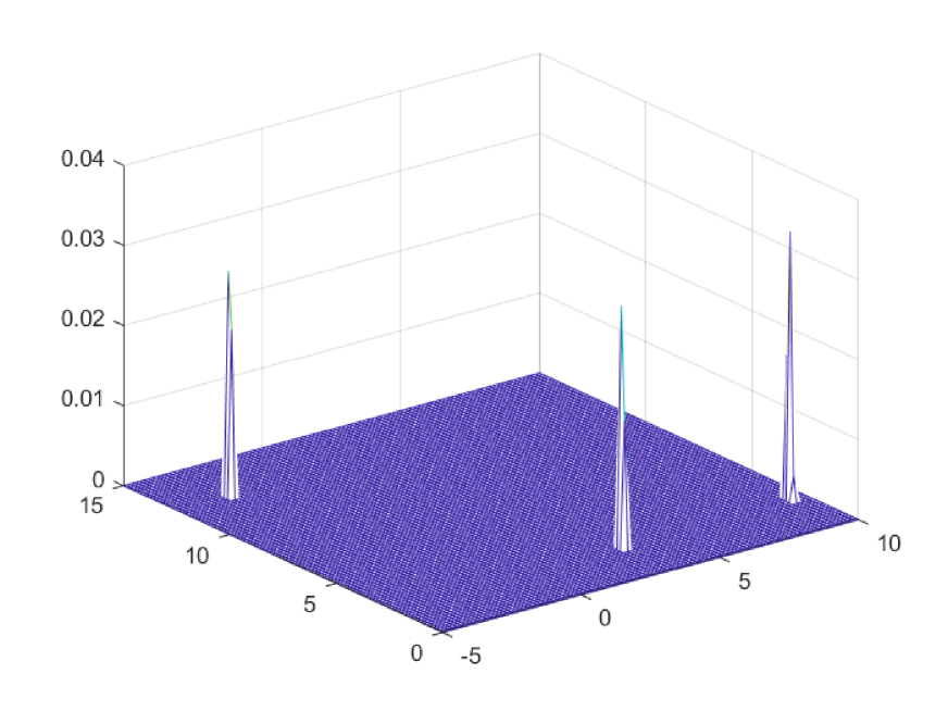
(b) steep at the end

Figure 1: Two types of EI in EGO

For the first drawback, we generate $N_{\rm min}$ points $\bm{u}_{i}$ and $v_{i}$ at once, where $N_{\rm min}$ is set to ensure the accuracy of the calculation. Instead of setting a fixed $M$, the rejection factor is defined by $\lambda_{i}=v_{i}\cdot\phi_{\rm max}/\phi(\bm{u}_{i})$. If the $(n-1)$-th smallest $\lambda_{(n-1)}\leq 1$, there are at least $n-1$ points accepted. We then sub-sample from the accepted samples by choosing the $n-1$ points with the smallest $\lambda_{i}$. This is equivalent to setting $M=\phi_{\rm max}/\lambda_{(n-1)}$. If $\lambda_{(n-1)}>1$, we set $M=\phi_{\rm max}$ and proceed with the rejection sampling.

To justify this, assume the target distribution is $f(\bm{x})$, the proposal distribution is $g(\bm{x})$, and $Mg(\bm{x})\geq f(\bm{x}),\forall\bm{x}$, $\lambda=\frac{Mg(\bm{x})}{f(\bm{x})}v,v\sim{\rm U}(0,1)$. Thus

$$\pi(\lambda|\textbf{accept},\bm{x})= \frac{\pi(\textbf{accept}|\lambda,\bm{x})\cdot\pi(\lambda|\bm{x})}{\pi(\textbf{accept}|\bm{x})}$$

$$= \frac{I_{0\leq\lambda\leq 1}\cdot f(\bm{x})/(Mg(\bm{x}))}{f(\bm{x})/(Mg(\bm{x}))}$$

$$= 1\cdot I_{0\leq\lambda\leq 1}\sim{\rm U}(0,1).$$ (3.1)

This means the distribution of $\lambda$, under the condition of acceptance, is ${\rm U}(0,1)$, which is independent of $\bm{x}$. The sub-samples according $\lambda$ then have the same distribution of the original samples.

For the second drawback, if we continue the above RS until $|U|\geq N_{\rm max}$ and the accepted samples are still not enough, we then turn to SIR, and $U$ in RS is directly regard as the pre-sample in SIR. $N_{\rm max}$ is set to accommodate the computational burden, and it is large enough to meet the requirements of SIR.

3.2 Calculation

The sampling and calculation can be carried out simultaneously to reduce the computational burden. Upon reviewing equation (2.2), if we take the proposal distribution $g(\cdot)$ as ${\rm U}(\Omega)$, then the pre-sample set $U$ in RS and SIR can be used to estimate $D^{2}(X,\phi,K)$. RS and SIR will be suitable for the calculation of $\hat{D}^{2}(X,\phi,K)$, and only minor modifications are required.

To take an acquisition function as a density, we need to normalize it by $f(\bm{x})=\phi(\bm{x})/\int_{\Omega}\phi(\bm{u})\mathrm{d}\bm{u}$, where $\int_{\Omega}\phi(\bm{u})\mathrm{d}\bm{u}$ can be estimated by

$$\int_{\Omega}\phi(\bm{u})\mathrm{d}\bm{u}\ \hat{=}\ \frac{1}{N}\sum_{i=1}^{N}\phi(\bm{u}_{i})\triangleq\frac{S_{\phi}}{N}.$$ (3.2)

Referring then to equation (2.2), $\hat{D}^{2}(X,\phi,K)$ can be written as

$$\hat{D}^{2}(X,\phi,K)= \frac{1}{S_{\phi}^{2}}\sum_{i,j=1}^{N}K(\bm{u}_{j},\bm{u}_{i})\cdot\phi(\bm{u}_{j})\cdot\phi(\bm{u}_{i})$$

$$-\frac{2}{nS_{\phi}}\sum_{i=1}^{n}\sum_{j=1}^{N}K(\bm{u}_{j},\bm{x}_{i})\cdot\phi(\bm{u}_{j})+\frac{1}{n^{2}}\sum_{i,j=1}^{n}K(\bm{x}_{j},\bm{x}_{i}).$$ (3.3)

As mentioned previously, sampling once without comparison is arbitrary and uncertain. We would like to generate several sets of samples as candidates, noted as $X^{(1)},X^{(2)},\dots,X^{(m)}$. Because the calculation above is very computationally intensive, we propose three measures to reduce this:

1. Reduce the calculation in pre-sampling. Every time we sample, keep $U$ unchanged and generate $X^{(k)}$. For RS, we only regenerate $v_{i}\sim{\rm U}(0,1)$ to screen $U$ again; For SIR, we resample directly from $U$. In this way, we only calculate $\phi(\bm{u}_{i})$ once, no matter how many times we sample.

2. Eliminate unnecessary calculations in $\hat{D}^{2}(X,\phi,K)$. Rewrite equation (3.2) as

   $$\hat{D}^{2}(X,\phi,K)= A_{1}(\phi,K)-\frac{2}{n}\sum_{i=1}^{n}A_{2}(\bm{x}_{i},\phi,K)+A_{3}(X,K),$$ (3.4)

   where $A_{1}(\phi,K)=\sum_{i,j=1}^{N}K(\bm{u}_{j},\bm{u}_{i})\cdot\phi(\bm{u}_{j})\cdot\phi(\bm{u}_{i})/S_{\phi}^{2}$ is irrelative to $X$, $A_{3}(X,K)=\sum_{i,j=1}^{n}K(\bm{x}_{j},\bm{x}_{i})/n^{2}$ is irrelative to $\phi$, and $A_{2}(\bm{x}_{i},\phi,K)=\sum_{j=1}^{N}K(\bm{u}_{j},\bm{x}_{i})\cdot\phi(\bm{u}_{j})/S_{\phi}$ is irrelative to other elements of $X$. Because $A_{1}$ is independent of $X$ and it is most computationally intensive, define

   $$\hat{D}_{-}^{2}(X,\phi,K)=-\frac{2}{n}\sum_{i=1}^{n}A_{2}(\bm{x}_{i},\phi,K)+A_{3}(X,K).$$ (3.5)

   We only compute equation (3.5) to compare the samples. If an exact $\hat{D}^{2}(X,\phi,K)$ is necessary for analysis, we calculate $A_{1}(\phi,K)$ once at the end, and add it to $\hat{D}_{-}^{2}(X,\phi,K)$.

3. Save the important calculation results. In addition to the candidate samples $X^{(k)}$ and their corresponding general discrepancies $D^{(k)}$, we save other calculation results for future optimization. Firstly, we save the sample set as $S=\cup_{k=1}^{m}X^{(k)}$. Next, because $A_{2}$ is only related to one site, $A_{2}(\bm{s}_{i},\phi,K)$ are saved as $A(i)$ for future optimization, where $\bm{s}_{i}$ are the corresponding elements of $S$. In addition, $\phi(\bm{u}_{i})$ calculated in the sampling process are saved as $\Phi(i)$ and are retrieved when calculating $K(\bm{u}_{j},\bm{x}_{i})\phi(\bm{u}_{i})$ in $A_{2}(\bm{s}_{i},\phi,K)$.

The complete processes of sampling and calculation are summarized in Algorithm 1.

Input: One-site acquisition function $\phi$, design size $n$, minimum sample size $N_{\rm min}$, maximum sample size $N_{\rm max}$, and number of candidate samples $m$

Output: Candidate samples $X^{(k)}$, sample set $S$, calculation results $D^{(k)}$, and $A$

1 let $N=N_{\rm min}$ and generate $U=\{\bm{u}_{i},i=1,\dots,N\}$ uniformly distributed on $\Omega$;

2 calculate $\phi_{i}=\phi(\bm{u}_{i}),i=1,\dots,N$ and save them as $\Phi$;

3 find $\phi_{\rm max}=\max\phi(\bm{x})=\phi(\bm{x}^{*})$ by some global optimization algorithm;

4 initialize $S=\{\bm{x}^{*}\},\ A=\{A_{2}(\bm{x}^{*},\phi,K)\}$;

5 for $k=1:m$ do

       $X^{(k)}=\{\bm{x}^{*}\}$;

        // maintain $\bm{x}^{*}\in X$

6       if $N<N_{\rm max}$ then // RS

7             generate $v_{i},i=1,\dots,N$ uniformly distributed on $(0,1)$;

8             calculate $\lambda_{i}=(v_{i}\cdot\phi_{\rm max})/\phi_{i},i=1,\dots,N$;

9             find the $(n-1)$-th smallest $\lambda_{i}=\lambda_{(n-1)}$;

10             if $\lambda_{(n-1)}\leq 1$ then // Subsampling from RS

11                   $X^{(k)}=X^{(k)}\cup\{\bm{u}_{i}|\lambda_{i}\leq\lambda_{(n-1)}\}$;

12                  

13            else // Continue to RS

14                   $X^{(k)}=X^{(k)}\cup\{\bm{u}_{i}|\lambda_{i}\leq 1\}$;

15                   while $|X^{(k)}|<n$ do

16                         $N=N+1$;

17                         generate $\bm{u}_{N}\sim{\rm U}(\Omega)$, $U=U\cup\{\bm{u}_{N}\},\ \Phi=\Phi\cup\{\phi_{N}=\phi(\bm{u}_{N})\}$;

18                         generate $v_{N}\sim{\rm U}(0,1)$;

19                         if $v_{N}\cdot\phi_{\rm max}\leq\phi_{N}$ then

20                               $X^{(k)}=X^{(k)}\cup\{\bm{u}_{N}\}$;

21                              

22                         end if

23                        if $N\geq N_{\rm max}$ then // Prepare for SIR

24                               calculate $w_{i}=\phi_{i}/\sum_{j=1}^{N}\phi_{j},i=1,\dots,N$;

25                               break and turn to SIR;

26                              

27                         end if

28                        

29                   end while

30                  

31             end if

32            

33      else // SIR

34             resample $\bm{x}^{(k)}_{2},\dots,\bm{x}^{(k)}_{n}$ from $U$ with the probability $(w_{1},\dots,w_{N})$;

35             $X^{(k)}=X^{(k)}\cup\{\bm{x}^{(k)}_{2},\dots,\bm{x}^{(k)}_{n}\}$;

36            

37       end if

38      $S=S\cup X^{(k)}$;

39       for $i=2:n$ do

40             calculate $A_{2}(\bm{x}^{(k)}_{i},\phi,K)$ by $\bm{x}^{(k)}_{i},U$ and $\Phi$;

41             $A=A\cup\{A_{2}(\bm{x}^{(k)}_{i},\phi,K)\}$;

42            

43       end for

44      calculate $D^{(k)}=\hat{D}_{-}^{2}(X^{(k)},\phi,K)$ by $X^{(k)}$ and $A_{2}(\bm{x}^{(k)}_{i},\phi,K)$;

45      

46 end for

calculate $\hat{D}_{+}=A_{1}(\phi,K)$ by $U$ and $\Phi$;

  // If exact $\hat{D}$ is necessary

47 For all $k$, $D^{(k)}=D^{(k)}+\hat{D}_{+}$;

Algorithm 1 Sample and Calculation of SCO

3.3 Optimization

After sampling and calculation, $X^{(1)},X^{(2)},\dots,X^{(m)}$ are still uncertain. To reduce the uncertainty of the final design $X^{*}$, we would like to optimize them under the criterion of general discrepancy. There are two difficulties in optimization. One is the large number of combinations of candidate sets; if we choose $X$ from $U$, all possible combinations are $\binom{N}{n}$, which makes optimization impractical. The other difficulty is the burden of calculation. No matter what kind of algorithm we choose, every time we generate a new design $X^{\rm new}$, calculating $\hat{D}^{2}(X^{\rm new},\phi,K)$, even $\hat{D}_{-}^{2}(X^{\rm new},\phi,K)$, is time-consuming.

Therefore, we need to optimize on a relative-small but reasonable set and make full use of the existing calculation results. Referring to equation (3.4), if $X^{\rm new}$ is generated from an old design $X^{\rm old}$ with general discrepancy $D^{\rm old}$ and all the sites are restricted in $S$, then $D^{\rm new}$ can be updated by

$$D^{\rm new}= D^{\rm old}+\frac{2}{n}\sum_{i\in I_{\rm old}}A(i)-\frac{2}{n}\sum_{i\in I_{\rm new}}A(i)-A_{3}(X^{\rm old},K)+A_{3}(X^{\rm new},K)$$

$$\triangleq D^{\rm old}+\Delta(X^{\rm new},X^{\rm old}),$$ (3.6)

where $D^{\rm old}$ and $A(i)$ are already known. We only calculate $A_{3}(X^{\rm old},K)$ and $A_{3}(X^{\rm new},K)$, and retrieve the changed terms of $A(i)$ in $I_{\rm old},I_{\rm new}$ to update $D$.

In the rest of this subsection, we introduce two algorithms to optimize $X^{*}$.

The genetic algorithm

The genetic algorithm (GA) is a classical intelligent optimization algorithm. We briefly introduce the process of the GA in Algorithm 2 and explain the operations of some important steps. For more details of the GA, one can refer to Goldberg, (1988).

Input: Data: candidate designs $X^{(k)}$, sample set $S$, calculation results $D^{(k)}$, and $A$;

Parameters: $l$ in fitness function, crossover probability $P_{\rm c}$, and mutation probability $P_{\rm m}$

Output: Optimal design $X^{*}$ and its corresponding $D^{*}$

1 initialize population: $Parents=\{X^{(1)},\dots,X^{(m)}\}$;

2 $k^{*}=\arg\min_{k}D^{(k)},X^{*}=X^{(k^{*})},D^{*}=D^{(k^{*})}$;

3 while Stopping criterion is not met do

       $Offspring=\{X^{*}\}$;

        // Retain the best individual

4       calculate the fitness function ${\rm Fit}(X)=D^{-l}(X)$;

5       while $|Offspring|<m$ do

6             $(Father,Mother)=Selection(Parents;{\rm Fit})$;

7             $Child=Crossover(Father,Mother;P_{\rm c})$;

8             $Child=Mutation(Child,S;P_{\rm m})$;

9             $D^{Child}=D^{Father}+\Delta(D^{Child},D^{Father})$;

10             $Offspring=Offspring\cup\{Child\}$;

11            

12       end while

13      update $X^{*}$ and $D^{*}$;

14       $Parents=Offspring$;

15      

16 end while

Algorithm 2 Genetic algorithm

• Fitness function—${\rm Fit}(X)=D^{-l}(X)$;

• Selection—two parents were selected using the roulette wheel method according to the ${\rm Fit}$ function; the best individual in each iteration remained unchanged to the next generation;

• Crossover—offspring were generated by exchanging the corresponding sites in parents with probability $P_{\rm c}$;

• Mutation—replace sites in offspring with a random site in $S$ with probability $P_{\rm m}$, except the first site $\bm{x}^{*}$.

The default parameters of the GA are set as $l=5,\ P_{\rm c}=0.5,\ P_{\rm m}=0.1$.

The switching algorithm

The switching algorithm (SA) is an efficient but local algorithm. In the design literature, it has been widely applied to fit the large space of optimization (Winker and Fang,, 1998; Fang et al.,, 2000; Chuang and Hung,, 2010). The main steps of the SA are shown in Algorithm 3, and it requires no parameters.

Input: Candidate designs $X^{(k)}$, sample set $S$, calculation results $D^{(k)}$, and $A$

Output: Optimal design $X^{*}$ and its corresponding $D^{*}$

1 $k^{*}=\arg\min_{k}D^{(k)},X^{*}=X^{(k^{*})},D^{*}=D^{(k^{*})}$;

2 do

3       for i=2:n do // Maintain $\bm{x}^{*}\in X^{*}$

4             find $\bm{s}^{*}=\arg\min_{\bm{s}\in S}\Delta(X_{i,\bm{s}}^{\rm switch},X^{*})$, where $X_{i,\bm{s}}^{\rm switch}=X^{*}\backslash\{\bm{x}_{i}\}\cup\{\bm{s}\}$;

5             if $\Delta^{*}=\Delta(X_{i,\bm{s}^{*}}^{\rm switch},X^{*})<0$ then

6                   $X^{*}=X_{i,\bm{s}^{*}}^{\rm switch}$;

7                   $D^{*}=D^{*}+\Delta^{*}$;

8                  

9             end if

10            

11       end for

12      

13while $X^{*}$ has changed;

Algorithm 3 Switch algorithm

From Algorithm 2 and 3, we can see both the GA and SA have the following properties:

• $\bm{x}^{*}$ is always the first site of $X^{*}$;

• $D^{*}$ is monotonically decreasing;

• every site in iterations is restricted in $S$;

• the inputs of Algorithm 2 and 3 are the outputs of Algorithm 1.

3.4 Summary

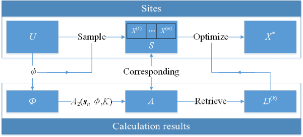
Figure 2: Flowchart of SCO

The flowchart of the SCO is shown in Figure 2, and we illustrate its process with an example. We build a Gauss process model according to $Y_{\rm data}=f_{\rm exp}(X_{\rm data})$, where $f_{\rm exp}$ is the Branin function (www.sfu.ca/~ssurjano/optimization.html), and $X_{\rm data}$ is the set of $4\times 4$ mesh points on $\Omega=[-5,10]\times[0,15]$. We then take EI as the acquisition function (Jones et al.,, 1998) and draw the contours of EI, see figure 3(a). The EI criterion captures the three extreme points of Branin function well. Then the pre-sample set $U$, sample set $S$, and the final design $X^{*}$ are plotted in different color. The size of $U$ is large, and it does not contain the features of $\phi$. Compared with the optimization from $U$, the optimization from $S$ can greatly reduce the number of possible combinations without losing the features of $\phi$, and $X^{*}$ is less uncertain than $S$. This point of view can be seen in Figure 3(b). We repeated 100 tests to compare the uncertainty of the two methods—the sampling-only method and the SCO method. We chose design sizes of 5,10, and 20 and compare their general discrepancies with the boxplots, which were grouped as S only-5, SCO-5 and so on. From Figure 3(b), we can see the uncertainty of the SCO designs were much less than the uncertainty of the sampling-only designs. The SCO designs were even better than sampling-only designs with the double sample size, in terms of general discrepancy.

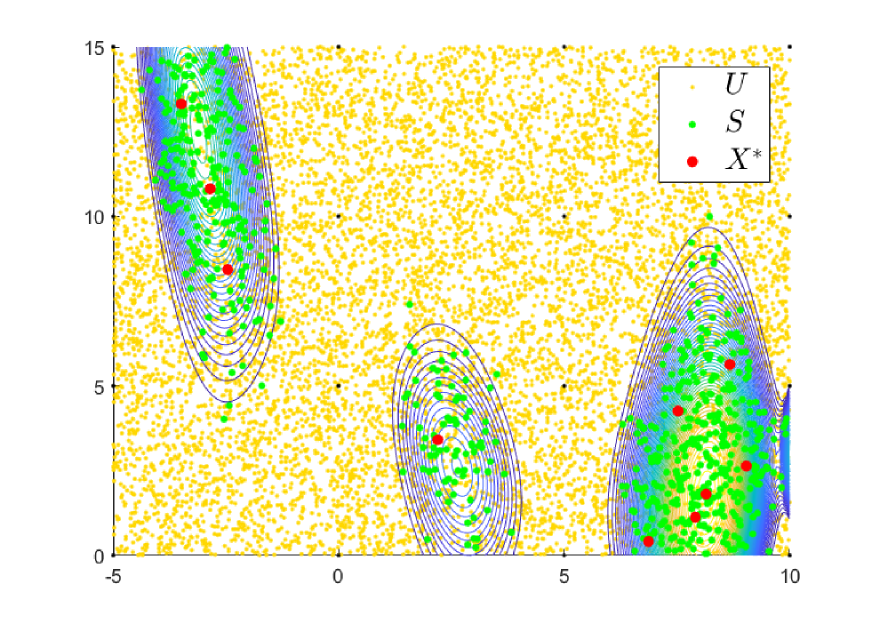
(a) Plots of different sets in SCO

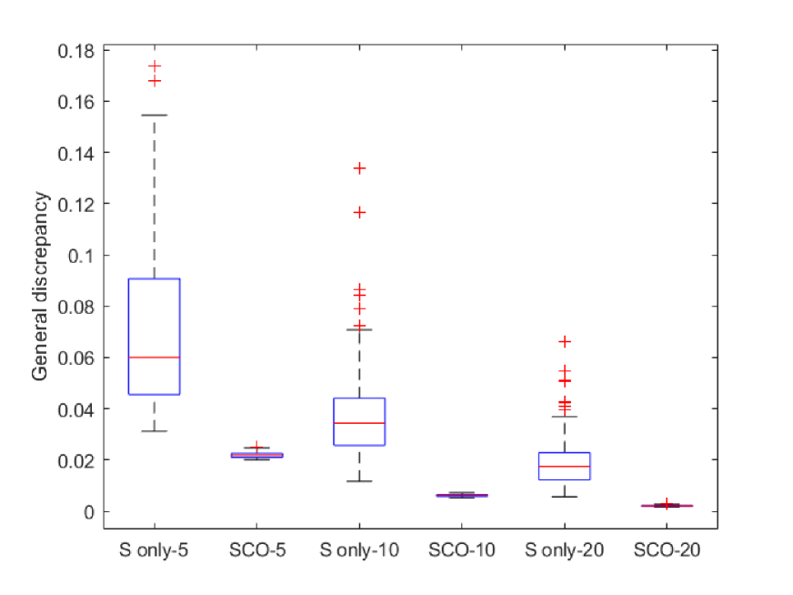
(b) Uncertainty of SCO and sampling-only

Figure 3: SCO example

4 Numerical results

In this section, we first study the efficiency of the GA and SA in the SCO. We then compare some batch Bayesian optimization methods from different perspectives.

4.1 GA and SA in SCO

In Section 3.3, we introduce the GA and SA for optimization. In order to compare their efficiencies, we generated the same inputs by Algorithm 1, then proceeded to optimization by Algorithms 2 and 3, respectively. The general discrepancies of the two algorithms are shown in Figure 4. The boxplots record the evolution of the population in the GA, and the red line records the switching design in the SA. From Figure 4, we can see that the SA converged faster than the GA, and the GA was able to provide slightly better results when the dimension was lower. In addition, the SA is monotonically decreasing within the iteration in theory; however, the GA is stochastic. Although the 4-th line in Algorithm 2 was adopted to ensure the monotonicity of the best individual, the population of the GA fluctuated greatly during evolution. In consideration of efficiency and stability, we chose the SA in the optimization of the SCO.

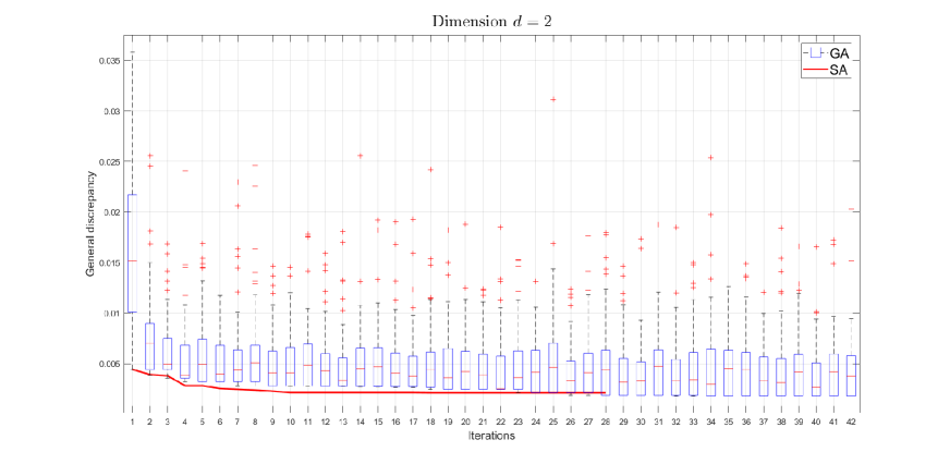
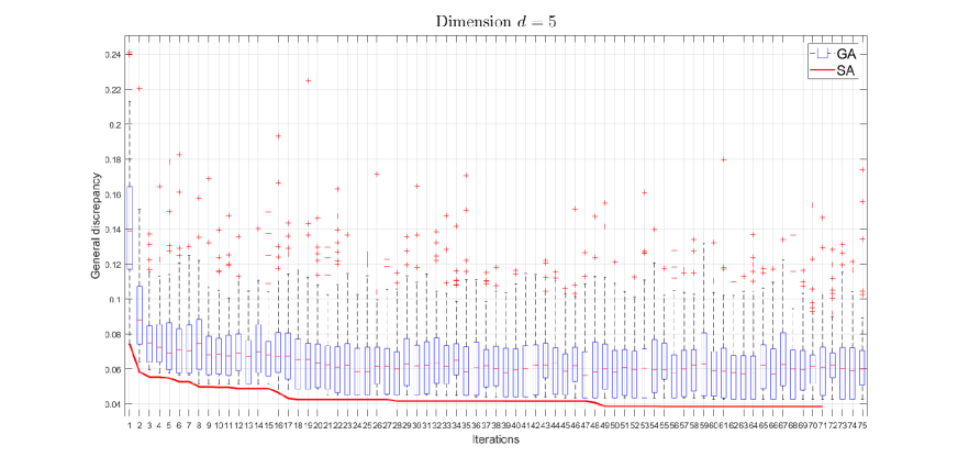
Figure 4: Comparison of the GA and SA in different dimensions

4.2 Efficiency of batch Bayesian optimization

As shown in the last section, the SCO design has good properties in terms of general discrepancy. However, can the advantage of general discrepancy be reflected in the batch Bayesian optimization? In this subsection, we will answer this question with numerical results. We compared the SCO method with some existing batch methods, including the $q$-EI method with kriging believer (KB) and constant liar minimum (CL-min) as heuristic strategies (Ginsbourger et al.,, 2010), multi-point sampling based on kriging (MPSK) method (Cai et al.,, 2017) and accelerated EGO (aEGO) method (Ning et al.,, 2020).

We compare SCO method with some existing batch methods, including $q$-EI method with “KB” and “CL-min” as heuristic strategies (Ginsbourger et al.,, 2010), MPSK method (Cai et al.,, 2017) and aEGO (Ning et al.,, 2020). Note that all these methods build a Gauss process model as a surrogate. However, KB and CL-min are based on a multi-point acquisition function; MPSK, aEGO, and SCO proposed in this article are sample-based methods. In order to reduce the contingency of the results, we used the Gaviano-Kvasov-Lera-Sergeyev (GKLS) method (Gaviano and Lera,, 1998; Gaviano et al.,, 2011) to generate several random functions as the objective. The parameters were set according to Gaviano et al., (2011); one of the GKLS functions in two dimensions is demonstrated in Figure 5. To compare the efficiency of the optimization, we define the average relative accuracy (ARA) as

$${\rm ARA}=\frac{1}{N_{\rm f}}\sum_{i=1}^{N_{\rm f}}\frac{y_{\rm min}^{(i)}-f_{\rm min}^{(i)}}{|f_{\rm min}^{(i)}|},$$ (4.1)

where $N_{\rm f}$ is the number of random functions, $f_{\rm min}^{(i)}$ is the optimal value of the $i$-th function, and $y_{\rm min}^{(i)}$ is the minimum response found by the algorithm.

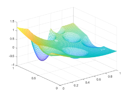
Figure 5: Demonstration of GKLS

First, we analyze the efficiency of the batch methods in different dimensions. We generated 100 functions for dimension $d=2,3,5,\ {\rm and}\ 10$. For each dimension, we started with same initial data sites $X_{\rm data}$ to optimize them. The number of $X_{\rm data}$ was set as $5\times d$, and $X_{\rm data}$ were constructed by uniform designs (Fang et al.,, 2018). We conducted five cycles of batch Bayesian optimization, with each batch size set as $n=5$. Figure 6 displays the ARAs of different batch methods in different dimensions. As to the methods based on a multi-point acquisition function, KB and CL-min performed well only in two dimensions. SCO and aEGO showed an advantage in higher dimensions, and SCO performed the best of all the sample-based methods.

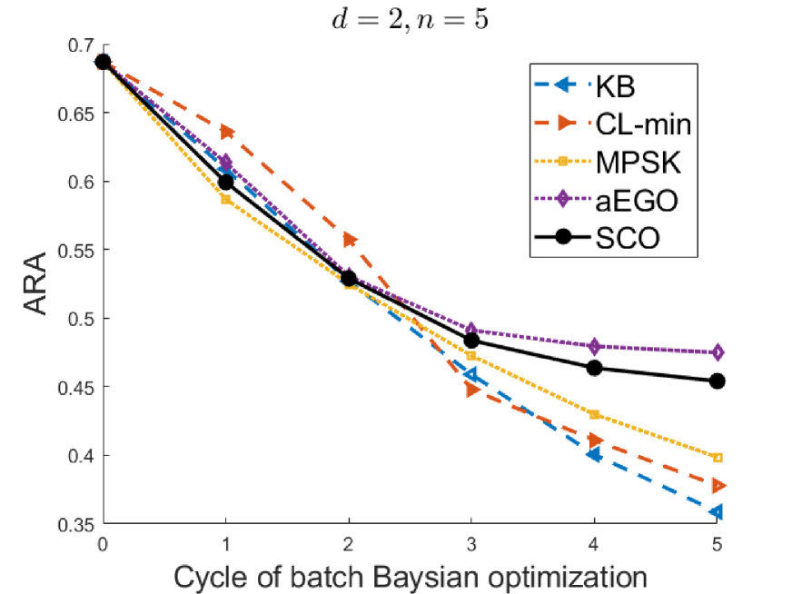
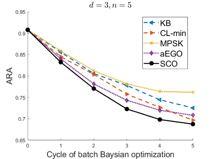
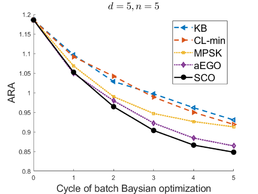
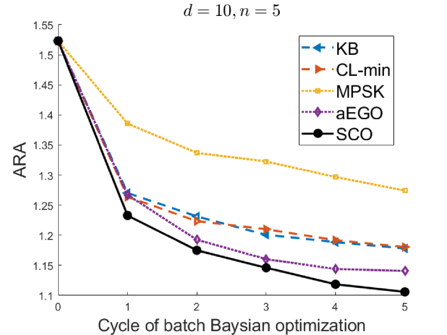
Figure 6: Comparison of batch Bayesian optimizations with different dimensions

Second, we analyzed the influence of batch size. For $d=4$, we conducted similar contrast experiments, but set $n=5,10,15,\ {\rm and}\ 20$. The ARAs are displayed in Figure 7. As the batch size increased, the difference between SCO and aEGO decreases, the ARAs of SCO and aEGO almost overlap when $n=20$. This illustrates that, the effect of calculation and optimization is not obvious when the batch size is large. It stands to reason that if we have enough experimental resources, experimental design would not matter. However, SCO is still most efficient among all sampling-based methods.

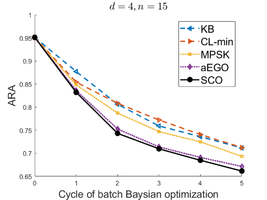
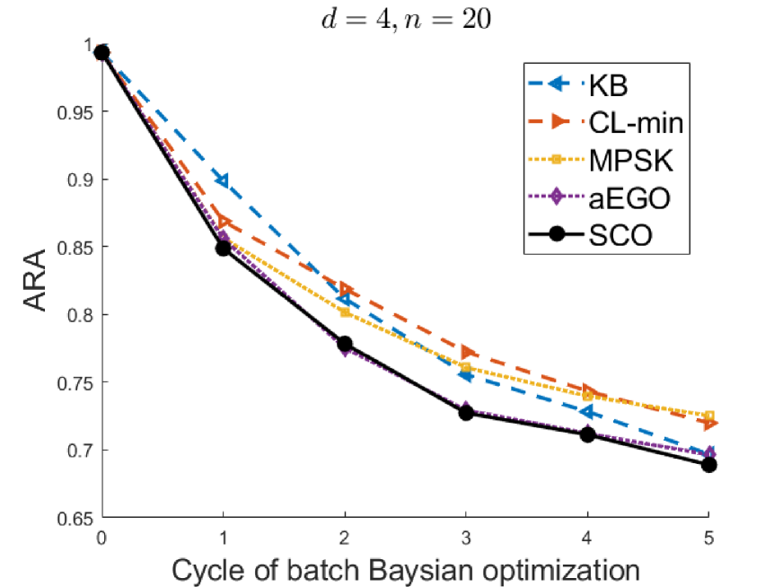
Figure 7: Comparison of batch Bayesian optimizations with different batch size

4.3 Application in radar interference experiment

The interference ability test of a certain type of radar is carried out. The interference method of releasing array decoy is adopted, as shown in Figure 8. The radar is fixed and the target is set at azimuth 0 and range $R$. After the radar is turned on, the target releases $N$ decoys spaced $d$, the decoys sail at speed $v$ and release interference signals at power $P$. The process of target recognition is recorded, and the interference is measured by azimuth angle $\theta$ of radar. The purpose of the experiment is to find the optimal strategy $(R,d,v,P)$ to maximize $\theta$ when $N$ is fixed.

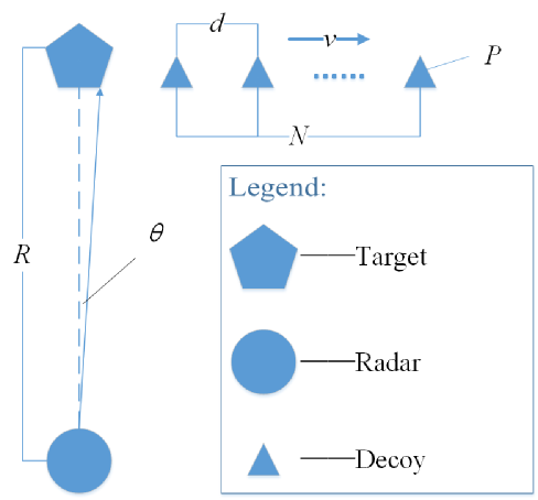
Figure 8: Schematic diagram of single experimental scene

Preliminary modeling is conducted based on previous experimental data and sequential experiments are carried out in the next stage. $n$ experiments can be carried out simultaneously in the same stage, as shown in Figure 9. In order to shorten the experimental period, the batch sequential experiments were carried out, and the SCO method was used to design the batch sequential experiments. Considering the resources of the experimental base, $n_{1}$ experiments were designed in the first stage. Analysis of the results showed that the experimental standard was still not met and further experiments were needed. Due to the change of the resources in the experimental base, $n_{2}$ sequential experiments were designed in the second stage. The SCO has the flexibility to deal with different batch size. The experimental results of the two stages are shown in Figure 10, where the interference $\theta$ is improved. Analyses confirmed that the results met the experimental standard.

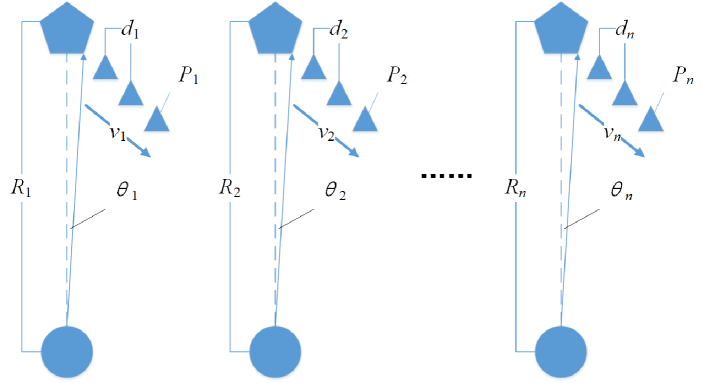
Figure 9: Schematic diagram of batch experimental scene

In this case, we made full use of experimental resources and met the experimental standard in two stages of batch experiments, which greatly shortened the experimental period. The SCO method is used for batch sequential experimental design, which is flexible and less uncertain. This means the SCO is more suitable for complex and high-cost experiments.

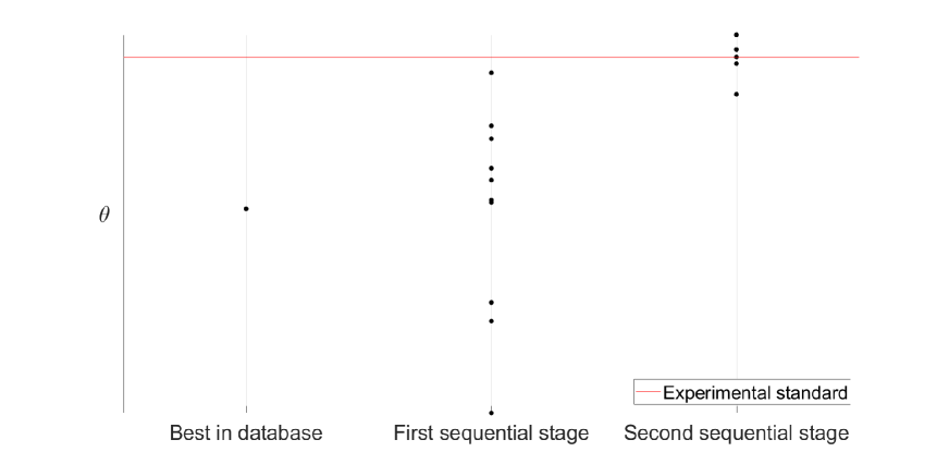
Figure 10: Experimental results

5 Conclusion and further discussion

This article introduced a sequential design method for batch Bayesian optimization. The main processes of this method include sampling-calculation-optimization (SCO). SCO is a sampling-based method that does not construct a new acquisition function but samples from the existing acquisition function. To reduce the uncertainty, the samples are optimized in the sense of general discrepancy. We have proposed several strategies to reduce the amount of computation and make the optimization possible. Numerical results show that the uncertainty of the SCO was much less than the sampling-only method. In addition, the batch Bayesian optimization with SCO was more efficient than other batch methods. Although we have introduced the SCO based on the Gaussian process model and the EI criterion, the method is also well-suited to other models and acquisition functions. Finally, the case of radar interference experiment shows the application value and scenario of SCO method.

In this article, the batch size is fixed and constrained by the experimental resource of every experimental period. In other kind of experiments, the batch size may be flexible and it is a part of the experimental design. In such case, how to design the batch size to experiment more efficiently remains to be further studied.

References

- Bishop, (2006) Bishop, C. M. (2006). Pattern Recognition and Machine Learning.
- Cai et al., (2017) Cai, X., Qiu, H., Gao, L., Yang, P., and Shao, X. (2017). A multi-point sampling method based on kriging for global optimization. Structural and Multidisciplinary Optimization, 56(1):71–88.
- Chen et al., (2014) Chen, R.-B., Hsu, Y.-W., Hung, Y., and Wang, W. (2014). Discrete particle swarm optimization for constructing uniform design on irregular regions. Computational Statistics and Data Analysis, 72:282–297.
- Chuang and Hung, (2010) Chuang, S. C. and Hung, Y. C. (2010). Uniform design over general input domains with applications to target region estimation in computer experiments. Computational Statistics and Data Analysis, 54(1):219–232.
- Fang et al., (2000) Fang, K. T., Lin, D. K., Winker, P., and Zhang, Y. (2000). Uniform design: Theory and application. Technometrics, 42(3):237–248.
- Fang et al., (2018) Fang, K.-T., Liu, M.-Q., Qin, H., and Zhou, Y.-D. (2018). Theory and Application of Uniform Experimental Designs.
- Fang et al., (2000) Fang, K. T., Ma, C. X., and Winker, P. (2000). Centered -discrepancy of random sampling and latin hypercube design.
- Fang and Wang, (1994) Fang, K.-T. and Wang, Y. (1994). Number-theoretic methods in statistics. Journal of The Royal Statistical Society Series A-statistics in Society, 158(1):189–190.
- Fang et al., (1994) Fang, K.-T., Wang, Y., and Bentler, P. M. (1994). Some applications of number-theoretic methods in statistics. Statistical Science, 9(3):416–428.
- Fu and Wang, (2002) Fu, J. C. and Wang, L. (2002). A random-discretization based monte carlo sampling method and its applications. Methodology and Computing in Applied Probability, 4(1):5–25.
- Gaviano et al., (2011) Gaviano, M., Kvasov, D. E., Lera, D., and Sergeyev, Y. D. (2011). Software for generation of classes of test functions with known local and global minima for global optimization. ACM Transactions on Mathematical Software, pages 469–480.
- Gaviano and Lera, (1998) Gaviano, M. and Lera, D. (1998). Test functions with variable attraction regions for global optimization problems. Journal of Global Optimization, 13(2):207–223.
- Ginsbourger et al., (2008) Ginsbourger, D., Riche, R. L., and Carraro, L. (2008). A multi-points criterion for deterministic parallel global optimization based on gaussian processes.
- Ginsbourger et al., (2010) Ginsbourger, D., Riche, R. L., and Carraro, L. (2010). Kriging is well-suited to parallelize optimization. pages 131–162.
- Goldberg, (1988) Goldberg, D. E. (1988). Genetic algorithms in search, optimization, and machine learning.
- Jones et al., (1998) Jones, D. R., Schonlau, M., and Welch, W. J. (1998). Efficient global optimization of expensive black-box functions. Journal of Global Optimization, 13(4):455–492.
- Li et al., (2020) Li, Y., Kang, L., and Hickernell, F. J. (2020). Is a transformed low discrepancy design also low discrepancy. arXiv preprint arXiv:2004.09887, pages 69–92.
- Niederreiter, (1992) Niederreiter, H. (1992). Random number generation and quasi-Monte Carlo methods.
- Ning et al., (2020) Ning, J., Xiao, Y., and Xiong, Z. (2020). Batch sequential adaptive designs for global optimization. arXiv preprint arXiv:2010.10698.
- Wang et al., (2004) Wang, L., Shan, S., and Wang, G. G. (2004). Mode-pursuing sampling method for global optimization on expensive black-box functions. Engineering Optimization, 36(4):419–438.
- Winker and Fang, (1998) Winker, P. and Fang, K.-T. (1998). Optimal -type designs. pages 436–448.
- Zhou and Fang, (2013) Zhou, Y.-D. and Fang, K.-T. (2013). An efficient method for constructing uniform designs with large size. Computational Statistics, 28(3):1319–1331.
- Zhou et al., (2012) Zhou, Y.-D., Fang, K.-T., and Ning, J.-H. (2012). Constructing uniform designs: A heuristic integer programming method. Journal of Complexity, 28(2):224–237.
- Zhou et al., (2013) Zhou, Y.-D., Fang, K.-T., and Ning, J.-H. (2013). Mixture discrepancy for quasi-random point sets. Journal of Complexity, 29(3):283–301.