Two-snapshot DOA Estimation via Hankel-structured Matrix Completion

Abstract

In this paper, we study the problem of estimating the direction of arrival (DOA) using a sparsely sampled uniform linear array (ULA). Based on an initial incomplete ULA measurements, our strategy is to choose a sparse subset of array elements for measuring the next snapshot. Then, we use a Hankel-structured matrix completion to interpolate for the missing ULA measurements. Finally, the source DOAs are estimated using a subspace method such as Prony on the fully recovered ULA. We theoretically provide a sufficient bound for the number of required samples (array elements) for perfect recovery. The numerical comparisons of the proposed method with existing techniques such as atomic-norm minimization and off-the-grid approaches confirm the superiority of the proposed method.

Index Terms—  Direction of arrival, matrix completion, non-unifrom sampling, off-the-grid compressed sensing, super-resolution.

1 Introduction

Conventional methods for estimating the direction of arrival (DOA) of multiple sources, mainly rely on the auto-correlation function of the received data, which requires the availability of samples of multiple snapshots [1]. Recent advances, however, have shown that the samples of even a single snapshot could be sufficient for estimating DOAs if the sources are sparsely present in the field of view [2]. To take advantage of the latter sparsity, it is common to use sparse recovery techniques in compressed sensing that require discretizing the range of angles (an angular grid). This comes with the drawback of grid mismatch error [3] which cannot be completely eliminated [4].

A super-resolution method is introduced [5] for estimating a sparse mixture of single-frequency signals based on uniform samples but without assuming any grid; the only constraint is a minimum separation between the frequencies. The method can be translated into a grid-less sparse DOA estimation technique based on a uniform array which is not an efficient array for source localization [6]. For sparse linear arrays (SLA) [7] proposed a grid-less sparse recovery method based on atomic-norm minimization (ANM). For perfect estimation, the method requires a minimum angular separation between the sources.

It is known that the Hankel matrix form of the samples of a ULA represents a low-rank matrix when the number of sources is small [8], which assists in estimating the DOAs. EMaC is a grid-less approach that extends this idea to a SLA [9, 10, 11]. The method essentially interpolates the sparse samples using matrix completion in order to achieve uniformly-spaced samples (SLA to ULA), and applies a standard super-resolution technique tailored for ULAs. Compared to ANM, EMaC is shown to retrieve more sources with the same number of samples.

Fig. 1: This figure shows an overview of the proposed DOA estimation method.

Besides the low-rank property of the matrix, most matrix completion techniques require the availability of uniform samples from the matrix. For non-uniformly sampled low-rank matrices, a two-phase sampling-recovery strategy is proposed in [12] for matrix-completion. However, the method does not work for matrices with structure such as Hankel matrices.

In this paper, we propose a new ULA sampling scheme tailored for the EMaC method; based on the received data of the first snapshot, we estimate the amount of possible information provided by each array element, and choose a small subset of most informative elements as the active ones for the next snapshot. Next, we employ the EMaC method to interpolate for the whole ULA and apply a standard DOA estimation technique. From simulation results, we observe that the proposed method could outperform the existing approaches.

For the proposed technique, we provide a theoretical sufficient bound for the number of required samples that lead to prefect recovery; the number is proportional to the average (and not the previously shown maximum in EMaC) of the leverage scores. These scores intuitively describe the amount information that each sample (array element) carry about the desired DOAs. Based on leverage scores of one snapshot, we decide how to choose array elements in the next snapshot. The samples obtained at array elements of the second snapshot are then interpolated to form a ULA. For the interpolation, we minimize the cost function introduced in [13] using an alternating direction method of multipliers (ADMM) approach. Simulation results show that the proposed method outperforms the existing methods such as ANM, EMaC, and a grid-based CS method.

Notations: Lowercase boldface letters (eg. $\mathbf{x}$) are used for column vectors and uppercase boldface letters (eg. $\mathbf{M}$) represent matrices. The set of all Hankel matrices of size $n\times d$ is shown by ${\cal H}(n,d)$. The $(n,d)$-Hankelization of a vector $\mathbf{x}$ of dimension $m=d+n-1\in\mathbb{N}$ is defined as $\mathbf{M}=\mathscr{H}(\mathbf{x})\in{\cal H}(n,d)$ where

$$\mathbf{M}_{ij}=\mathbf{x}_{|i+j-1|},$$ (1)

that is, $\mathscr{H}(\mathbf{x})$ is the Hankel matrix appropriately constructed from the elements of the vector $\mathbf{x}$ by placing the $i^{\rm th}$ element in $\mathbf{x}$ identically on the $i^{\rm th}$ anti-diagonal of $\mathbf{M}$. Note the Hankelization of a vector is sometimes referred to as Hankel structure matrix, see [13].

${\rm rank}(\cdot)$, , $\cdot^{\rm H}$, $\|.\|_{\rm F}$ and $\|.\|_{*}$ stand for the rank operator, Hermitian operator (conjugate-transpose), the Frobenius norm and the nuclear-norm of a matrix, respectively. Also, we use $\mathds{1}_{\mathbf{x},\Omega}$ to represent the indicator function where it equals to $\mathbf{x}_{i}$ for $i\in\Omega$ and infinity otherwise.

2 System Model

Suppose an array with $m$ elements which are chosen from $n$ possible uniformly spacing locations along a line ($m\leq n$). In the uniform setting, each element has distance $d$ from its neighbors. The phase shift of the received signal (with wavelength $\lambda$) from a source at angle $\phi$ at $k$-th antenna element relative to the first element (the reference) is found by $a_{k}(\phi)=\exp{\big{(}-{\rm j}\tfrac{2\pi}{\lambda}kd\sin(\phi)\big{)}}$. Similarly, the overall received signal from sources located at angles $\phi_{1},\dots,\phi_{r}$ is

$$y_{k}=\sum_{\ell=1}^{r}b_{\ell}a_{k}(\phi_{\ell}).$$ (2)

where $b_{\ell}$s are complex numbers that encode both the received power from the sources and their phase values with respect to a reference. To summarize, we define $\tau_{\ell}=\frac{d}{\lambda}\sin(\phi_{\ell})$ which converts the measurements model (2) into $y_{k}=\sum_{\ell=1}^{r}b_{\ell}{\rm e}^{-{\rm j}2\pi\tau_{\ell}k}$. Now, the DOA problem is to estimate $\tau_{1},\dots,\tau_{r}$ by observing $y_{\Omega_{1}},\dots,y_{\Omega_{m}}$, where $\Omega\subset\{1,\dots,n\}$. In vectorial form, we represent the full ULA samples as $\mathbf{y}=[y_{1},\dots,y_{n}]^{T}$ and denote the observed (available) samples by $\mathbf{y}_{\rm o}=\mathcal{P}_{\Omega}(\mathbf{y})$ where the projection operator $\mathcal{P}_{\Omega}$ equals to $\mathbf{y}[{k}]$ for $k\in\Omega$ and zero for the $k\not\in\Omega$.

3 Proposed method

As explained earlier, we assume that a full ULA is available, however, due to implementation and timing budgets, the data of only a few ($m$) array elements are measured and processed. At the time of receiving the first snapshot, a predefined subset $\Omega\subset\{1,\dots,n\}$ of array elements are active. Based on the measured data $\mathcal{P}_{\Omega}(\mathbf{y}_{1})$, we assign a score (leverage scores) to each array element in the ULA which roughly shows the amount of information that the element conveys about the targets. For the second snapshot, we activate the $m$ most significant array elements $\widetilde{\Omega}\subset\{1,\dots,n\}$ according to the scores. Next, we use EMaC to predict the data of the $n-m$ unmeasured array elements. Finally, we estimate the DOAs based on the full ULA data ($\widehat{\mathbf{y}_{2}}$).

The concept of leverage scores was introduced in [12] for enhancing the performance of matrix completion in an adaptive sampling scenario. It is known that sampling the matrix elements with probabilities proportional to the leverage scores reduces the number of required samples for perfect recovery. Unfortunately, the leverage scores defined in [12] are not applicable to Hankel-structured matrices, as the elements in a Hankel matrix are repeated multiple times and cannot have independent scores. Here, we adapt the scoring concept to Hankel matrices.

Definition 1.

For an odd integer $n$ and  $\mathbf{x}\in\mathbb{C}^{n}$, let $\mathbf{U}_{N\times r}\bm{\Sigma}_{r\times r}(\mathbf{V}_{N\times r})^{\rm H}$ be the singular value decomposition (SVD) of the Hankelization of $\mathbf{x}$, $\mathscr{H}(\mathbf{x})$, where $N=(n+1)/{2}$ and $r={\rm rank}(\mathscr{H}(\mathbf{x}))$. We define the leverage scores $\{\mu_{k}\}_{k=1}^{n}$ as

$$\mu_{k}:=\frac{n}{r}\max\left\{\|\mathbf{U}^{\rm H}\mathbf{A}_{k}\|_{\rm F}^{2},\|\mathbf{A}_{k}\mathbf{V}^{\rm H}\|_{\rm F}^{2}\right\},$$ (3)

for $k\in\{1,\dots,n\}$ by setting $\mathbf{A}_{k}:=\frac{\mathscr{H}(\mathbf{e}_{i}^{n})}{\|\mathscr{H}(\mathbf{e}_{i}^{n})\|_{\rm F}}$, where $\mathbf{e}_{i}^{n}$ denotes the $i$th canonical basis of $\mathbb{R}^{n}$. We should note that the set $\{\mathbf{A}_{k}\}_{k=1}^{n}$ spans the space of $N\times N$ Hankel matrices.

Since the data of the full ULA is not available, we need to approximate the leverage scores in Def. 1 from the SLA associated with $\Omega$. This approximation can be obtained from the SVD of $\mathscr{H}\big{(}\mathcal{P}_{\Omega}(\mathbf{y}_{1})\big{)}$ i.e. $\widetilde{\mathbf{U}}\widetilde{\bm{\Sigma}}(\widetilde{\mathbf{V}})^{\rm H}$ for computing the approximate leverage scores $\widetilde{\mu}_{k}$, which determine the active array elements $\widetilde{\Omega}$ for the next snapshot.

Once the set $\widetilde{\Omega}$ has been identified, we consider the following matrix completion problem to interpolate values at missing locations:

$$\widehat{\mathbf{y}}_{2}=\underset{\mathbf{g}\in\mathbb{C}^{n}}{\rm argmin}~{}~{}~{}\|\mathscr{H}({\mathbf{g}})\|_{*},\ \ {\rm s.t.}~{}~{}~{}\mathcal{P}_{\widetilde{\Omega}}(\mathbf{g})=\mathcal{P}_{\widetilde{\Omega}}(\mathbf{y}_{2}).$$ (4)

The optimization problem in (4) is a convex relaxation of matrix rank minimization. In order to reduce the computational complexity of the minimization, we solve the nuclear norm minimization (4) using a SVD-free method. As shown in [14], we can replace the nuclear norm of a matrix $\mathbf{A}$, i.e. $\|\mathbf{A}\|_{*}$, with the $\underset{\mathbf{U},\mathbf{V}}{\min}\|\mathbf{U}\|_{\rm F}^{2}+\|\mathbf{V}\|_{\rm F}^{2}$ subject to $\mathbf{A}=\mathbf{UV}^{\rm H}$. As a result, (4) can be represented as

$$\underset{\mathbf{U},\mathbf{V},\mathbf{g}\in\mathbb{C}^{n}}{\rm argmin}~{}\|\mathbf{U}\|_{\rm F}^{2}+\|\mathbf{V}\|_{\rm F}^{2}~{}{\rm s.t.}~{}\mathcal{P}_{\widetilde{\Omega}}(\mathbf{g})=\mathcal{P}_{\widetilde{\Omega}}({\mathbf{y}}),{\rm and}~{}\mathbf{g}=\mathbf{UV}^{\rm H}.$$

Next, we combine the two constraints to apply the ADMM method in the following cost function:

$$L_{\rho}(\mathbf{U},\mathbf{V}, \mathbf{g},\bm{\Lambda})=\|\mathbf{U}\|_{\rm F}^{2}+\|\mathbf{V}\|_{\rm F}^{2}+\mathds{1}_{\mathbf{g},\Omega}$$

$$+\rho\|\mathscr{H}(\mathbf{g})-\mathbf{UV}^{\rm H}+\bm{\Lambda}\|_{\rm F}^{2},$$ (5)

where $\mathds{1}_{\mathbf{g},\Omega}$ denotes the indicator function. Also, $\rho$ is a positive scalar and the Lagrange multiplier $\bm{\Lambda}$ has the same size as $\mathscr{H}(\mathbf{g})$. To implement the ADMM technique, we shall minimize $L_{\rho}(\mathbf{U},\mathbf{V},\mathbf{g},\bm{\Lambda})$ sequentially in terms of its argument in turn. We skip the details here. Although minimizing $L_{\rho}$ is not a convex program, the analysis in [15] guarantees the convergence when the penalty parameter $\rho$ is sufficiently large. Finally, the DOAs can be estimated using standard super-resolution methods, see [16].

Algorithm 1 Hankel interpolation using ADMM

1:Input:

2: Observed samples $\mathcal{P}_{\Omega}(\mathbf{y}_{1})\in\mathbb{C}^{n}$ and corresponding coordinates $\Omega\subset[n]$,

3: Parameters ${\rho}$ for the augmented Lagrangian form

4:Output:

5: Completed Vector $\widehat{{\mathbf{y}}}_{2}\in\mathbb{C}^{n}$.

6:procedure Hankel_ Interpolation(${\mathcal{P}_{\Omega}(\mathbf{y}_{1})},{\rho}$)

7:     Estimate leverage scores $\mu_{k}$ by (3) using $\mathcal{P}_{\Omega}(\mathbf{y}_{1})$

8:     Construct $\widetilde{\Omega}$ using $\mu_{k}$ and change sampled locations

9:     Get new samples $\mathcal{P}_{\widetilde{\Omega}}(\mathbf{y}_{2})$

10:     Solve ADMM problem in (3) (consider $\rho$ as its input) by proposed method in [13] to find full array data $\widehat{\mathbf{y}}_{2}$

11:     return $\quad\widehat{\mathbf{y}}_{2}$

12:end procedure

(a)

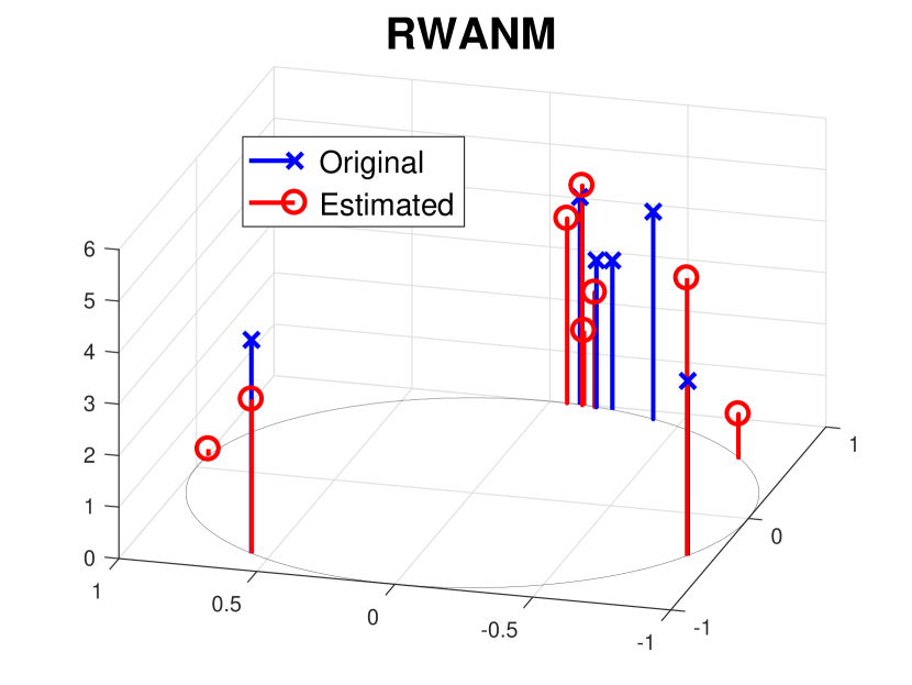
(b)

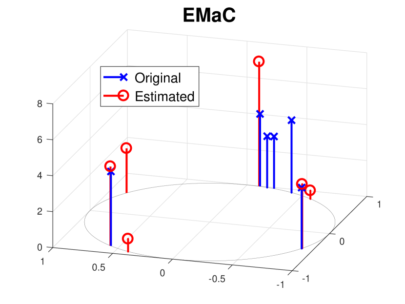
(c)

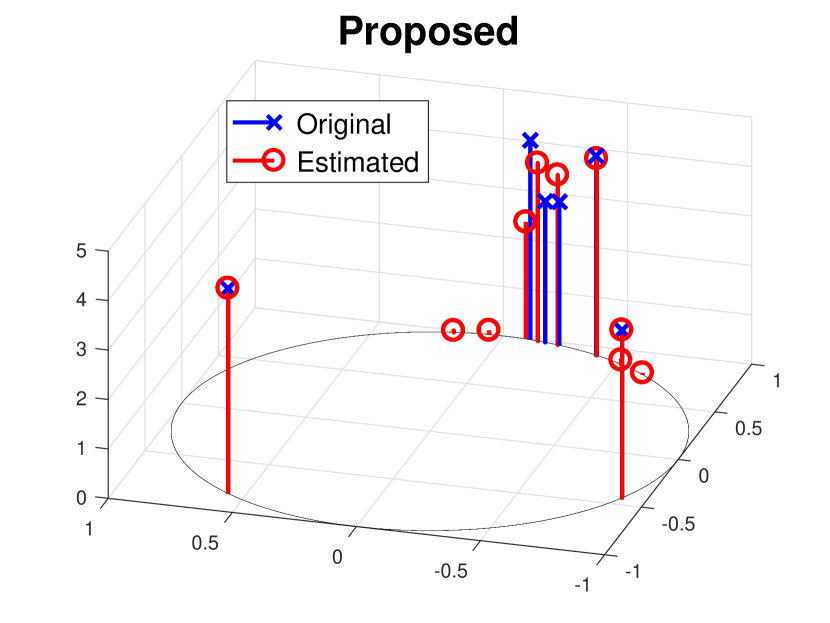
(f)

Fig. 2: Comparison of the performance in DOA estimation; the height of the bars shows the received signal power, and base circle in each figure represents the $360^{\circ}$ angular space. Here, we have $6$ sources with one almost collocated triplets.

4 Guarantee for prefect recovery

Below, we provide a theoretical result for the number of required samples. For this purpose, we use the simplifying assumption that the sampled set $\Omega$ is formed by selecting $i\in\{1,\dots,n\}$ with probability $p_{i}$ independently of $j\neq i$. We now show that if $p_{i}$s are large enough, we can correctly recover the DOAs.

Theorem 1.

Let $\mathbf{y}\in\mathbb{C}^{n}$ be the vector of true samples of the ULA for an $r$-sources. $\mathbf{y}$ can be recovered with probability no less than $1-n^{-10}$ from the measurements on the SLA $\mathcal{P}_{\widetilde{\Omega}}(\mathbf{y})$ where $\Omega$ i.e. index set of the location of the antenna elements in the SLA are randomly chosen by uniformly drawing the indices from $[n]$ by solving the optimization in (4) if

$$p_{k}\geq\min\Big{\{}1~{},~{}\frac{\max\big{(}c{\mu}_{k}r^{2}\log^{3}{(n)}\,\,,\,\,1\big{)}}{n}\Big{\}},$$ (6)

and $\frac{1}{8\log(n)}\leq\min\{\|\mathbf{U}\mathbf{U}^{\mathsf{H}}\mathbf{e}_{1}^{d}\|_{\rm F}^{2},\|\mathbf{e}_{n}^{n-d+1}\mathbf{V}\mathbf{V}^{\mathsf{H}}\|_{\rm F}^{2}\},$ where $d$ is the pencil parameter used in the Hankel operator and $\mathbf{U},\mathbf{V}$ are the unitary matrices of SVD of $\mathscr{H}(\mathbf{y})$. Also $\mu_{k}$ is the leverage score of Definition 1 of the paper and $c>0$ is a universal constant.

As the expected number of total samples is given by $\sum_{k}p_{k}$, Theorem 1 shows that the number of required samples for prefect recovery is proportional to the $\frac{\sum_{k=1}^{n}{\mu_{k}}}{n}$ instead of $\max_{k}\mu_{k}$ in [9].

5 Simulations

In this section, we compare the proposed sampling algorithm with some off-the-shelf single-snapshot DOA estimation methods like ANM [17], RWANM [18] and EMaC [9].

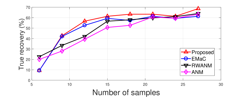
(a)

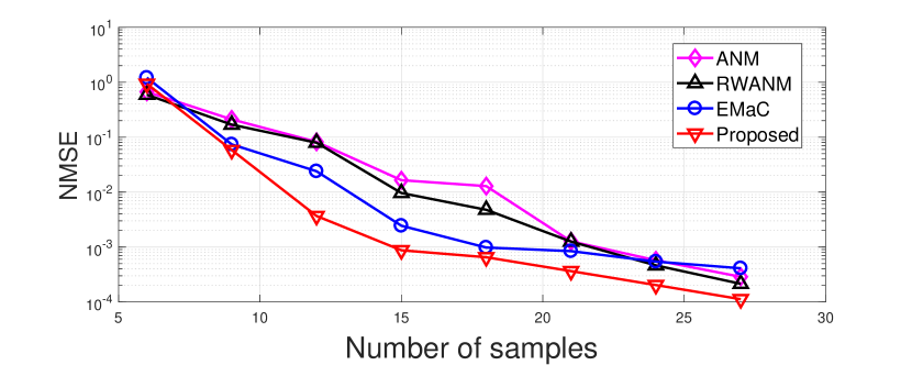
(b)

Fig. 3: Effect of the array size. The SLA interpolation normalized mean square errors are depicted for different array sizes. The source setup includes $5$ sources with two co-angled pairs.

Note that all methods, like the proposed one, inherently include an array completion procedure. After this first phase, subspace methods like Prony [16] and super-resolution [5] are employed to estimate the DOAs.

We assess the effect of the proposed non-uniform array selection for EMaC with standard uniform sampling in terms of array interpolation and DOAs estimation. To show the improvement, we also compare the modified EMaC with the other grid-less algorithms like ANM and RWANM that outperform standard EMaC. Moreover, to fairly assess array selection, the algorithms only used one snapshot of data to estimate the DOAs. In fact, we want to assess the effectiveness of the array selection in comparison with uniformly at random selection. Note that this strategy is only designed for the Hankel structure in the EMaC algorithm.Furthermore, we use only one snapshot for estimating the leverage scores; however, it is possible to increase this number in practical scenarios to alleviate system imperfections such as noise.

In the experiments, the ULA elements are placed on integer multiples of $\lambda/2$, where $\lambda$ is the wavelength. In the first snapshot, we randomly select $\Omega$ (active elements) and use the samples for estimating the leverage scores defined in (3). Before the second snapshot, we activate ULA elements with probabilities proportional to the estimated leverage scores. For other methods, ULA elements are activated with uniform probability. In the ADMM algorithm, the value of $\rho$ should be sufficiently large to guarantee the convergence: in our simulations we choose $\rho=10^{3}$. Next, we consider two simulation scenarios:

(i) Fig. 2 – DOA estimation: we consider an array with an aperture equal to $51\lambda/2$ ($52$ elements) and activate $12$ elements in each snapshot. In Fig. 2, both the original DOAs and the estimated ones are plotted. This scenario includes $6$ sources from which $3$ are almost collocated. As shown in this figure, existing methods are unable to distinguish or detect seemingly collocated sources correctly.The proposed method, however, resolves all source locations correctly, although with some false-positive sources with very low amplitudes.

(ii) Fig. 3 – effect of the array size: In the second experiment, we aim to evaluate the overall performance of the proposed algorithm against other methods for different number of active array elements. As before, we consider a $51\lambda/2$ aperture size for the uniform array; further, we uniformly select $6$ to $27$ elements for the SLA while we have $6$ sources at angles $\{-23.80^{\circ}$,$15.60^{\circ}$,$16.20^{\circ}$, $-17.53^{\circ}$,$18.13^{\circ}\}$ with amplitudes $\{3.31$,$3.2$,$2.13$,$3.14$,$3.56\}$, respectively. We call a detection correct, if for the source angle $\theta$ and its estimated version $\hat{\theta}$ we have that $|\sin{\theta}-\sin{\hat{\theta}}|\leq 0.005$. In Fig. 3-(a), we plot the rate of correct source recovery as a function of the SLA size (active elements). For each curve, the average results over $100$ random realization of the SLA elements are reported. We can see that the performance of the proposed sampling strategy outperforms the standard EMaC method, as well as other uniform algorithms such as ANM and RWANM. The recovery rate also increases as the number of the elements increase.Fig. 3-(b) depicts the normalized MSE of the estimated ULA’s missed elements in the SLA. Almost for any array size, the proposed method has the smallest NMSE value.

6 Conclusion

We studied a new ULA sampling method based on leverage scores in the two-snapshot DOA estimation problem. We proposed an approach that initially determines optimal array elements for matrix completion using the received data from the first snapshot. Next, it applies the EMaC method on the second snapshot data to find the DOAs. The sampling method is numerically observed to outperform EMaC, and other state-of-the-art grid-less DOA estimation techniques which have better performance than EMaC. besides, we provided a theoretical guarantee for perfect estimation.

References

- [1] R. O. Schmidt, “A signal subspace approach to multiple emitter location and spectral estimation,” Ph.D. dissertation, Stanford University, 1981.
- [2] M. Jin, G. Liao, and J. Li, “Joint DOD and DOA estimation for bistatic MIMO radar,” Signal Processing, vol. 89, no. 2, pp. 244–251, 2009.
- [3] Y. Chi, L. L. Scharf, A. Pezeshki, and A. R. Calderbank, “Sensitivity to basis mismatch in compressed sensing,” IEEE Transactions on Signal Processing, vol. 59, no. 5, pp. 2182–2195, 2011.
- [4] Z. Yang, L. Xie, and C. Zhang, “A discretization-free sparse and parametric approach for linear array signal processing,” IEEE Transactions on Signal Processing, vol. 62, no. 19, pp. 4959–4973, 2014.
- [5] E. J. Candès and C. Fernandez-Granda, “Towards a mathematical theory of super-resolution,” Communications on pure and applied Mathematics, vol. 67, no. 6, pp. 906–956, 2014.
- [6] G. Xu and Z. Xu, “Compressed sensing matrices from Fourier matrices,” IEEE Transactions on Information Theory, vol. 61, no. 1, pp. 469–478, 2014.
- [7] G. Tang, B. N. Bhaskar, P. Shah, and B. Recht, “Compressed sensing off the grid,” IEEE transactions on information theory, vol. 59, no. 11, pp. 7465–7490, 2013.
- [8] Y. Hua, “Estimating two-dimensional frequencies by matrix enhancement and matrix pencil,” IEEE Transactions on Signal Processing, vol. 40, no. 9, pp. 2267–2280, 1992.
- [9] Y. Chen and Y. Chi, “Robust spectral compressed sensing via structured matrix completion,” IEEE Transactions on Information Theory, vol. 60, no. 10, pp. 6576–6601, 2014.
- [10] S. Razavikia, A. Amini, and S. Daei, “Reconstruction of binary shapes from blurred images via hankel-structured low-rank matrix recovery,” IEEE Transactions on Image Processing, vol. 29, pp. 2452–2462, 2019.
- [11] S. Razavikia, H. Zamani, and A. Amini, “Sampling and recovery of binary shapes via low-rank structures,” in 2019 13th International conference on Sampling Theory and Applications (SampTA). IEEE, 2019, pp. 1–4.
- [12] Y. Chen, S. Bhojanapalli, S. Sanghavi, and R. Ward, “Completing any low-rank matrix, provably,” The Journal of Machine Learning Research, vol. 16, no. 1, pp. 2999–3034, 2015.
- [13] J. C. Ye, J. M. Kim, K. H. Jin, and K. Lee, “Compressive sampling using annihilating filter-based low-rank interpolation,” IEEE Transactions on Information Theory, vol. 63, no. 2, pp. 777–801, 2016.
- [14] N. Srebro, “Learning with matrix factorizations,” Ph.D. dissertation, MIT, 2004.
- [15] M. Hong, Z.-Q. Luo, and M. Razaviyayn, “Convergence analysis of alternating direction method of multipliers for a family of nonconvex problems,” SIAM Journal on Optimization, vol. 26, no. 1, pp. 337–364, 2016.
- [16] R. Prony, “Essai expérimental et analytique sur les lois de la dilatabilité des fluides élastiques et sur celles de la force expansive de la vapeur de l’eau et de la vapeur de l’alkool, à différentes températures,” J. de l’Ecole Polytechnique, vol. 1, pp. 24–76, 1795.
- [17] B. N. Bhaskar, G. Tang, and B. Recht, “Atomic norm denoising with applications to line spectral estimation,” IEEE Transactions on Signal Processing, vol. 61, no. 23, pp. 5987–5999, 2013.
- [18] Z. Yang and L. Xie, “Enhancing sparsity and resolution via reweighted atomic norm minimization,” IEEE Transactions on Signal Processing, vol. 64, no. 4, pp. 995–1006, 2015.