Global convergence and acceleration of projection methods for feasibility problems involving union convex sets

Abstract

We prove global convergence of classical projection algorithms for feasibility problems involving union convex sets, which refer to sets expressible as the union of a finite number of closed convex sets. We present a unified strategy for analyzing global convergence by means of studying fixed-point iterations of a set-valued operator that is the union of a finite number of compact-valued upper semicontinuous maps. Such a generalized framework permits the analysis of a class of proximal algorithms for minimizing the sum of a piecewise smooth function and the difference between pointwise minimum of finitely many weakly convex functions and a piecewise smooth convex function. When realized on two-set feasibility problems, this algorithm class recovers alternating projections and averaged projections as special cases, and thus we obtain global convergence criterion for these projection algorithms. Using these general results, we derive sufficient conditions to guarantee global convergence for several projection algorithms for solving the sparse affine feasibility problem and a feasibility reformulation of the linear complementarity problem. Notably, we obtain global convergence of both the alternating and the averaged projection methods to the solution set for linear complementarity problems involving $P$-matrices. By leveraging the structures of the classes of problems we consider, we also propose acceleration algorithms with guaranteed global convergence. Numerical results further exemplify that the proposed acceleration schemes significantly improve upon their non-accelerated counterparts in efficiency.

Keywords. fixed point algorithm; proximal methods; alternating projections; averaged projections; linear complementarity problem; union convex set; nonconvex feasibility problems; nonconvex optimization; global convergence

1 Introduction

Given two closed sets $S_{1}$ and $S_{2}$ in a Euclidean space $\mathbb{E}$, the two-set feasibility problem formulated below involves finding a point in the intersection of $S_{1}$ and $S_{2}$:

$$\text{find}~{}w\in S_{1}\cap S_{2}.$$ (FP)

Given $w^{0}\in\mathbb{E}$, the method of alternating projections Eq. MAP

$$w^{k+1}\in(P_{S_{2}}\circ P_{S_{1}})(w^{k}),$$ (MAP)

and the method of averaged projections Eq. MAveP

$$w^{k+1}\in\left(\frac{P_{S_{1}}+P_{S_{2}}}{2}\right)(w^{k})$$ (MAveP)

are two classical projection methods for solving Eq. FP. Here, $P_{S}:\mathbb{E}\rightrightarrows S$ denotes the projector onto a closed set $S$ given by

$$P_{S}(w)\coloneqq\{y\in S:{\left\|{y-w}\right\|}\leq{\left\|{z-w}\right\|}\text{ for all }z\in S\},\quad\forall w\in\mathbb{E},$$ (1.1)

which may contain more than one point when $S$ is nonconvex. While global convergence of Eq. MAP and Eq. MAveP to a point in $S_{1}\cap S_{2}$ is well-understood when the sets involved are convex [Auslender, 1969, Brègman, 1965], the global convergence even just to a superset of the solution set of Eq. FP of MAP and MAveP for nonconvex feasibility problems largely remains unknown. To date, only local convergence results are known for the general nonconvex setting (see Drusvyatskiy and Lewis [2019], Lewis et al. [2009].

Meanwhile, a special nonconvex structure known as union convexity has recently been observed in some application problems. A set is said to be a union convex set if it is expressible as a finite union of closed convex sets [Dao and Tam, 2019]. A prominent example is the problem of finding a sparse solution to a linear system $Aw=b$ with $A\in{\rm I}\!{\rm R}^{m\times n}$ and $b\in{\rm I}\!{\rm R}^{m}$ under the constraint $\|w\|_{0}\leq s$ for some $s\geq 0$. This is known as the sparse affine feasibility problem (SAFP), which can be cast as a feasibility problem Eq. FP with

$$S_{1}=\{w\in{\rm I}\!{\rm R}^{n}:Aw=b\},\quad\text{and}\quad S_{2}=A_{s}\coloneqq\{w\in{\rm I}\!{\rm R}^{n}:\|w\|_{0}\leq s\}.$$ (1.2)

$A_{s}$ is known as the “sparsity set”, which is a finite union of linear subspaces [Dao and Tam, 2019, Hesse et al., 2014]. More recently, Alcantara et al. [2023] studied the general absolute value equation (GAVE) $Ax+B|x|=c$ with $A,B\in{\rm I}\!{\rm R}^{m\times n}$ and $c\in{\rm I}\!{\rm R}^{m}$, which can be naturally reformulated as Eq. FP with $S_{1}=\{(x,y)\in{\rm I}\!{\rm R}^{n}\times{\rm I}\!{\rm R}^{n}\}:Ax+By=c\}$, and $S_{2}=\{(x,y)\in{\rm I}\!{\rm R}^{n}\times{\rm I}\!{\rm R}^{n}\}:y=|x|\}$ is a finite union of half-spaces. In these works, Eq. MAP was used to solve the feasibility formulation, but its global convergence for GAVE is not fully understood except for homogeneous cases, while a quite restrictive assumption is used for the SAFP.

Following the approach in Alcantara et al. [2023], we may also reformulate the linear complementarity problem (LCP) as a union convex set feasibility problem. Given $M\in{\rm I}\!{\rm R}^{n\times n}$ and $b\in{\rm I}\!{\rm R}^{n}$, the LCP requires finding a point $x\in{\rm I}\!{\rm R}^{n}$ that satisfies

$$x\geq 0,\qquad Mx-b\geq 0,\qquad\text{and}\qquad\langle x,Mx-b\rangle=0.$$ (1.3)

This problem encompasses many applications such as bimatrix games and equilibrium problems, and notably includes quadratic programming as a special case [Cottle et al., 1992]. Many algorithms have been proposed for solving the system Eq. 1.3; we refer interested readers to Cottle et al. [1992], Facchinei and Pang [2003] for a comprehensive survey of theory and algorithms. Meanwhile, a different class of algorithms can be derived through a simple reformulation of the LCP Eq. 1.3 as a feasibility problem. Indeed, through introducing an additional variable $y\coloneqq Mx-b$ and letting $w\coloneqq(x,y)$, the LCP Eq. 1.3 is equivalent to Eq. FP with

$$S_{1} =\{w\in{\rm I}\!{\rm R}^{2n}~{}:~{}Aw=b\}\quad\text{with}\quad A\coloneqq[M,\quad-I_{n}]\in{\rm I}\!{\rm R}^{n\times 2n},$$ (1.4)

$$S_{2} =\{w\in{\rm I}\!{\rm R}^{2n}~{}:w_{j}\geq 0,\;w_{n+j}\geq 0,\;w_{j}w_{n+j}=0,\;\forall j\in\{1,2,\dotsc,n\}\}.$$

Despite the special union convex structure of the involved sets of these feasibility problems, determining the conditions under which the algorithms Eq. MAP and Eq. MAveP are globally convergent remains to be an open problem, except for very specific instances of SAFP and GAVE. This work aims to show global convergence of the classical projection algorithms applied to feasibility problems involving union convex sets.

1.1 Our approach

To prove global convergence, we interpret the projection methods Eq. MAP and Eq. MAveP as proximal algorithms for solving optimization problems. In particular, we consider the structured optimization problem

$$\min_{w\in\mathbb{E}}\quad V(w)\coloneqq f(w)+g(w)-h(w),$$ (OP)

where $V$ is level-bounded, $f$ is the pointwise minimum of a finite number of functions with Lipschitz-continuous gradients, $g$ is the pointwise minimum of (weakly, strongly) convex functions, and $h$ is a continuous real-valued convex function expressible as the pointwise maximum of continuously differentiable convex functions. We denote by $I_{f}$, $I_{g}$ and $I_{h}$ the collections of functions that define the pieces of $f$, $g$ and $h$, respectively. That is, $f=\min_{f_{i}\in I_{f}}f_{i}$, $g=\min_{g_{i}\in I_{g}}g_{i}$, and $h=\max_{h_{i}\in I_{h}}h_{i}$. We say that $f_{i}\in I_{f}$ is active at a point $w\in\mathbb{E}$ if $f(w)=f_{i}(w)$. Note that $f$ is not necessarily smooth, and $g$ is not necessarily a convex function. For this structured problem, we introduce the following proximal-type algorithm

$$w^{k+1}\in T_{\rm prox}^{\lambda}(w^{k})\coloneqq{\rm prox}_{\lambda g}\left(w^{k}-\lambda f^{\prime}(w^{k})+\lambda h^{\prime}(w^{k})\right),$$ (1.5)

where ${\rm prox}_{\lambda g}:\mathbb{E}\rightrightarrows\mathbb{E}$ is the proximal operator, and the mappings $f^{\prime},h^{\prime}:\mathbb{E}\rightrightarrows\mathbb{E}$ respectively map a point to the set of all gradients of functions in $I_{f}$ and $I_{h}$ that are active at the given point.

We will show that under proper choices of the functions $f$, $g$ and $h$ satisfying the said piecewise structures, the algorithms Eq. MAP and Eq. MAveP can be realized from the proximal algorithm Eq. 1.5. Hence, by deriving general conditions under which Eq. 1.5 is globally convergent, we obtain as a corollary the global convergence of Eq. MAP and Eq. MAveP for union convex set feasibility problems. Through this reformulation, we can greatly simplify the task of finding sufficient conditions for guaranteeing global convergence on the parameters for our motivational problems of the sparse affine feasibility problem, general absolute value equations, and the linear complementarity problem.

Our convergence analysis of the proximal algorithm Eq. 1.5 involves studying the global convergence of the more general fixed point iterations defined by

$$w^{k+1}\in T(w^{k}),~{}k\geq 0,$$ (FPI)

where $T:\mathbb{E}\rightrightarrows\mathbb{E}$ is a set-valued operator that generalizes the properties of $T_{\rm prox}^{\lambda}$ for our considered setting. In particular, we consider what we call a union upper semicontinuous operator $T$, which is a set-valued map that can be decomposed as a finite union of upper semicontinuous operators, referred to as the individual operators of $T$ (see Definition 3.2). To establish the global convergence of Eq. FPI, we assume the existence of a Lyapunov function associated with the operator $T$, in the sense defined in Definition 4.1. In the case of the optimization problem Eq. OP, we show that the objective function itself is the associated Lyapunov function for $T_{\rm prox}^{\lambda}$.

1.2 Contributions

The main contributions of this work include global convergence results as follows.

• Global convergence of fixed point iterations. Under the assumption that a Lyapunov function for an upper semicontinuous operator $T$ exists, we show in Theorem 4.2 that any accumulation point of the iterations Eq. FPI is a fixed point of $T$, that is, it belongs to the set

  $$\operatorname*{Fix}(T)\coloneqq\{w\in\mathbb{E}:w\in T(w)\}.$$

  We further note in Example 4.3 that without the existence of a Lyapunov function, this result may not hold in general. Moreover, we also prove in Theorem 4.4 that when the individual operators of $T$ are calm at an accumulation point and $T$ is single-valued there, global convergence of the full sequence holds.

• Global convergence of the proximal algorithm and fixed point set characterization. Using the general theory, we establish in Theorem 5.7 the global convergence of the proximal algorithm Eq. 1.5 to fixed points of $T_{\rm prox}^{\lambda}$ for suitable stepsize $\lambda$ by showing that the objective function of Eq. OP is a Lyapunov function for $T_{\rm prox}^{\lambda}$. This is stronger than the global subsequential results typically obtained in the literature. To relate the importance of fixed points to the optimization problem Eq. OP, we show in Theorem 5.10 that

  $$\text{local minima of \lx@cref{creftype~refnum}{eq:minconvex_optimization}}\subset\operatorname*{Fix}(T_{\rm prox}^{\lambda}).$$

  Meanwhile, criticality is a notion more traditionally used for providing necessary optimality conditions for Eq. OP, and we show in Theorem 5.11 that under a simple regularity assumption,

  $$\text{local minima of \lx@cref{creftype~refnum}{eq:minconvex_optimization}}\subset\operatorname*{Fix}(T_{\rm prox}^{\lambda})\subset\text{critical points of \eqref{eq:minconvex_optimization}}.$$

  Our convergence guarantee is thus stronger than the traditional subsequential convergence to critical points only.

  The setting we consider for Eq. OP subsumes the ones studied in prior works such as Dao and Tam [2019], Wen et al. [2018]. Consequently, our framework significantly extends these existing works to a wider class of optimization problems. More importantly, we obtain results concerning global convergence of the full sequence, which are stronger than the local or global subsequential convergence in existing works.

• Global convergence of classical projection algorithms for union convex set feasibility problems. Under certain coercivity assumptions, a consequence of the above general framework is that Eq. MAveP and a relaxed version of Eq. MAP, given by

  $$w^{k+1}\in P_{S_{2}}((1-\lambda)w^{k}+\lambda P_{S_{1}}(w^{k}))$$ (1.6)

  with $\lambda\in(0,1)$, are both globally convergent to fixed points of their defining operators, as shown in Section 5.3.

We use the above results to determine conditions on the matrices involved in SAFP, LCP, and GAVE under which the algorithms Eq. MAP, Eq. 1.6, and Eq. MAveP are globally convergent. We point out that despite the availability of the above powerful tools for the general case, the analysis for these specific problems still requires quite some rigor, especially for proving the global convergence of Eq. MAP for LCP. In particular, the following are our contributions for these feasibility problems.

• New (and old) projection algorithms for the sparse affine feasibility problem with global convergence guarantees. In Theorems 6.3 and 6.4, we establish global convergence for the projected gradient algorithm and the relaxed method of alternating projections Eq. 1.6 applied on the sparse affine feasibility problem. The conditions we impose on the affine constraint are significantly looser than the ones used in existing works such as Beck and Teboulle [2011], Hesse et al. [2014], yet we still obtain global convergence to candidate solutions of the feasibility problem. One can also easily derive the same results as direct consequences of our analysis under the assumptions used in these works. In addition, our general framework is also capable of developing new algorithms with ease, and we thus derive several new algorithms for sparse affine feasibility, with similar global convergence guarantees.

• New projection algorithms for the linear complementarity problem and square absolute value equations with global convergence guarantees. As for the LCP Eq. 1.3, we show in Theorem 6.7 that Eq. MAveP and the relaxed Eq. MAP given in (1.6) are globally convergent to fixed points when $M$ is a nondegenerate matrix, i.e., a matrix with nonzero principal minors. Moreover, local $Q$-linear convergence holds for Eq. 1.6.

  We further show that for matrices with strictly positive principal minors, also known as $P$-matrices, global convergence of Eq. MAveP and relaxed MAP Eq. 1.6 to the actual solution set of the feasibility reformulation is guaranteed. More significantly, we prove in Corollary 6.10 that global convergence also holds for the original iterations given by Eq. MAP (as opposed to Eq. 1.6), which is a rare result for nonconvex feasibility problems. Similar to the sparse affine feasibility problem, we also present several other globally convergent projection-based algorithms for solving the LCP based on its feasibility reformulation. For GAVE involving square matrices $A$ and $B$, the results for the LCP can be easily adapted by reformulating the former as a linear complementarity problem with $M=(A^{\top}+B^{\top})(A^{\top}-B^{\top})^{-1}$, as discussed in [Alcantara et al., 2023, Remark 2.18].

This work also contributes in the algorithmic side to propose acceleration schemes that greatly improve the efficiency of fixed-point iterations and projection algorithms.

• Two Acceleration Schemes. We present a general acceleration scheme for the fixed point iterations Eq. FPI using the Lyapunov function with guaranteed global subsequential convergence proved in Theorem 4.2. Taking advantage of the piecewise structures of $f$, $g$ and $h$ in Eq. OP (or of the union convex sets $S_{1}$ and $S_{2}$), we further derive accelerated proximal algorithms whose global subsequential convergence follows from the general case in Section 5.5. In Section 7, we demonstrate empirically that our acceleration methods significantly improve the performance of their non-accelerated versions. The proposed acclerated algorithms also outperform existing methods in our experiments.

1.3 Outline

In Section 2, we discuss works related to the different problem settings described above, and highlight the major differences with and improvements over the existing works of this paper. Mathematical preliminaries are summarized in Section 3. General tools concerning global convergence of the fixed point iterations Eq. FPI with union upper semicontinuous $T$ are derived in Section 4. Global convergence of the proximal algorithm Eq. 1.5 and characterization of the fixed points of $T_{\rm prox}^{\lambda}$ are established in Section 5. We illustrate in Section 5.3 how to derive the projection methods Eq. MAP and Eq. MAveP from these proximal algorithms, and we also derive another algorithm that was considered in Bauschke et al. [2013]. Our accleration schemes for the proximal algorithms are proposed in Section 5.5. In Section 6, we present a unified analysis of six projection algorithms for SAFP and LCP. Section 7 presents numerical experiments, and concluding remarks are given in Section 8.

2 Related works and further contributions

We now compare and contrast our contributions with existing results in the literature on related topics.

Fixed point problems.

For the fixed point algorithm Eq. FPI, similar classes of operators $T$ that can be expressed as a union of a finite number of set-valued operators were studied by Dao and Tam [2019], Tam [2018]. In these works, continuous (single-valued) individual operators, namely nonexpansive and paracontracting maps, were considered. On the other hand, the setting we consider involves set-valued upper semicontinuous individual operators, and thus subsumes that in these prior works. When each individual operator is nonexpansive, local convergence of Eq. FPI was already established in Dao and Tam [2019]. Our contribution described in (I) shows that a missing ingredient to extend this into a global result is the existence of a coercive Lyapunov function (see Definitions 4.1 and 4.2). With a coercive Lyapunov function, single-valuedness of the union operator at an accumulation point and calmness of the individual operators at the same point are sufficient for guaranteeing global full convergence.

Optimization.

For structured optimization problems of the form Eq. OP, a traditional setting considered in previous works involves a function $f$ that has a Lipschitz continuous gradient, a proper closed convex function $g$, and a continuous real-valued convex function $h$ [Liu and Takeda, 2022, Wen et al., 2018]. This setting contains a class of regularized optimization problems that are usually motivated from statistics and machine learning. In these applications, $f$ is a data-dependent loss function and $g-h$ represents a difference-of-convex regularizer such as the smoothly clipped absolute deviation, minimax concave penalty, transformed $\ell_{1}$, or the logarithmic penalty. However, under these assumptions on $f$, $g$ and $h$, it is difficult to interpret the projection methods Eq. MAP and Eq. MAveP for union convex set Eq. FP as proximal algorithms for solving a certain Eq. OP, as one shall see in this work.

When $|I_{f}|=|I_{g}|=|I_{h}|=1$ and $g$ is a convex function, the algorithmic operator of Eq. 1.5 reduces to a single-valued operator $T_{\rm prox}^{\lambda}={\rm prox}_{\lambda g}\circ(Id-\lambda\nabla f+\lambda\nabla h)$, which corresponds to the algorithm studied in [Wen et al., 2018, Section 4.2], and the authors established its global convergence under the Kurdyka-Łojasiewicz (KL) assumption with a quadratic regularization on the objective function $V$. On the other hand, when $|I_{f}|=1$, $|I_{h}|=0$ and all the functions in $I_{g}$ are convex, $T_{\rm prox}^{\lambda}$ simplifies to $T_{\rm prox}^{\lambda}={\rm prox}_{\lambda g}\circ(Id-\lambda\nabla f)$, which is the forward-backward algorithm considered in Dao and Tam [2019], where only local convergence to fixed points of $T_{\rm prox}^{\lambda}$ has been established. Hence, this paper provides a unifying setting for the above works, and is the first attempt to understand the global convergence of the algorithm Eq. 1.5 when $f$, $g$, and $h$ are piecewise functions described in Section 1.1.

Nonconvex feasibility problems.

Due to difficulties that come with nonconvexity, the existing body of literature on projection algorithms for solving nonconvex feasibility problems mainly focuses on local convergence. For instance, the local convergence of MAP for finding the intersection of union convex sets was established in [Dao and Tam, 2019]. Using the same framework, one can also obtain local convergence of MAveP. Global convergence for these algorithms on nonconvex sets largely remains unknown, and our present work shows that coercivity assumptions are sufficient to attain global convergence for the special case of union convex sets.

Local linear convergence of MAP and MAveP for general nonconvex feasibility problems was studied in [Lewis et al., 2009] using the notion of strong regularity of points in the solution set $S_{1}\cap S_{2}$. In the present work, we also establish local linear convergence of MAP (see Proposition 5.9 and Section 5.3) but under a Lipschitz continuity assumption that is more easily verifiable and potentially weaker than strong regularity. For example, for the feasibility formulation of LCP, the proof of Proposition A.3 shows that if $M$ is a nondegenerate matrix and $w^{*}\in S_{1}\cap S_{2}$ is a nondegenerate point (in the sense of Definition A.2), then $S_{1}$ and $S_{2}$ have a “linearly regular intersection at $w^{*}$” as defined in Lewis et al. [2009] see also the proof of [Alcantara et al., 2023, Theorem 3.19]. Consequently, MAP is locally linearly convergent to $w^{*}$ by [Lewis et al., 2009, Theorem 5.16]. However, it should be pointed out that nondegeneracy of $w^{*}$ is essential to guarantee this result, but this is not verifiable a priori. Theorem 6.13, on the other hand, asserts that a linear rate is achievable whether or not $w^{*}$ is nondegenerate.

Sparse affine feasibility problem.

Convergence analyses of existing methods for the sparse affine feasibility problem usually require near-orthonormality conditions on the matrix $A$ in Eq. 1.2, such as the restricted isometry property (RIP) introduced in Candès and Tao [2005]. A more general condition subsuming the RIP is the scalable restricted isometry property (SRIP): A matrix $A\in{\rm I}\!{\rm R}^{m\times n}$ is said to satisfy the SRIP of order $(d,\alpha)$ if there exist $\mu_{d}\geq\nu_{d}>0$ with $\mu_{d}/\nu_{d}<\alpha$ such that

$$\nu_{d}\|w\|^{2}\leq\|Aw\|^{2}\leq\mu_{d}\|w\|^{2},\quad\forall w\in A_{d}.$$ (2.1)

In Beck and Teboulle [2011], the authors showed that the projected gradient algorithm with stepsize $\lambda\in(0.5\nu_{2s}^{-1},\mu_{2s}^{-1}]$ is globally convergent to the solution set if the SRIP of order $(2s,2)$ holds. This algorithm coincides with Eq. 1.5 with $f(w)=\|Aw-b\|^{2}/2$, $g=\delta_{A_{2}}$, and $h\equiv 0$.

On the other hand, Eq. MAP was used in Hesse et al. [2014] to solve SAFPs, and its global convergence was proved under any of the following conditions on $A$:

1. $AA^{\mathsf{T}}=I_{m}$ and the SRIP of order $(2s,2)$ holds with $\mu_{2s}=1$; or

2. there exists a constant $\nu_{2s}\in(0.5,1]$ such that $\nu_{2s}\|w\|^{2}\leq\|A^{\dagger}Aw\|^{2}$ for all $w\in A_{2s}$.

Meanwhile, we show in Theorem 6.4 that we can attain global convergence to fixed points of both the projected gradient algorithm with stepsize $\lambda\in(0,1/\|A\|^{2})$ and of the relaxed MAP given by Eq. 1.6 with $\lambda\in(0,1)$ under a significantly weaker assumption that there exists $\mu_{s}>0$ such that

$$\nu_{s}\|w\|^{2}\leq\|Aw\|^{2},\quad\forall w\in A_{s}.$$ (2.2)

This assumption is much weaker than the SRIP of order $(2s,2)$ used in Beck and Teboulle [2011] in two ways: (i) we have no restriction on the parameter $\nu_{s}$, and (ii) the inequality Eq. 2.2 is required to hold over $A_{s}$ only, instead of over their larger set $A_{2s}$. Similarly, condition (C1) used in Hesse et al. [2014] for Eq. MAP is much stronger than Eq. 2.2, as it not only assumes the SRIP as in Beck and Teboulle [2011], but also requires semi-orthogonality of $A$ and a specific value for $\mu_{2s}$. Condition (C2), on the other hand, is also much stronger than Eq. 2.2, since it needs to hold over the larger set $A_{2s}$ and requires a specific range of values for $\nu_{2s}$. Together with the fact that $\|A^{\dagger}Aw\|^{2}\leq\|A^{\dagger}\|^{2}\|Aw\|^{2}$, (C2) implies Eq. 2.2 for some $\nu_{s}$. Since the assumption Eq. 2.2 we use is significantly weaker than those in Beck and Teboulle [2011], Hesse et al. [2014], we obtain global convergence to fixed points only. However, under those same stronger conditions, we can obtain easily global convergence to the solution set as a direct consequence of our framework.

To our knowledge, Eq. MAP and the projected gradient algorithm discussed above are the only available methods for SAFP in the literature. We show in Theorem 6.3 that Eq. MAveP is also globally convergent for SAFP under the same assumption of Eq. 2.2. Moreover, we also present other new algorithms in Section 6.1 that also attain global convergence under the same condition.

Linear complementarity problem.

There are two well-known algorithms for LCP that, similar to Eq. MAP and Eq. MAveP, are also projection-based: the basic projection algorithm (BPA) and the extragradient algorithm (EGA) [see Facchinei and Pang, 2003, Algorithms 12.1.1 and 12.1.9]). BPA is suitable when the matrix $M$ associated with the LCP Eq. 1.3 is positive definite, in the sense that $x^{\mathsf{T}}Mx>0$ for all nonzero vector $x$. On the other hand, EGA can handle a positive semidefinite $M$. Meanwhile, all the algorithms we propose in Section 6.2 are new projection methods for LCP with guaranteed global convergence to fixed points for LCPs with a nondegenerate matrix and guaranteed global convergence to the solution set for LCPs with a $P$-matrix. The classes of nondegenerate and $P$-matrices both include the set of positive definite matrices, and therefore the proposed methods can solve those LCPs that are in the scope of BPA. On the other hand, both the sets of nondegenerate and $P$-matrices contain matrices that are not positive semidefinite, and therefore lead to LCP problems solvable by our approaches but not EGA.

3 Notations and Definitions

We let $w_{+}\coloneqq\max\{w,0\}$, where the maximum is taken componentwise. $\operatorname*{Ran}(A)$ and $\operatorname*{Ker}(A)$ denote respectively the range and the kernel of a matrix $A\in{\rm I}\!{\rm R}^{p\times q}$. We let $\|A\|$ denote the operator norm of $A$. We also let $[q]=\{1,\dots,q\}$, and for $\Lambda\subset[q]$, we denote by $A_{:,\Lambda}$ the submatrix of $A$ containing all of its columns indexed by $\Lambda$, $A_{\Lambda,\Lambda}$ the submatrix of $A$ containing its rows and columns indexed by $\Lambda$, and $\Lambda^{c}$ the complement set $\{i:i\in[q],i\notin\Lambda\}$. Given $w\in{\rm I}\!{\rm R}^{q}$, $w_{\Lambda}\in{\rm I}\!{\rm R}^{\lvert\Lambda\rvert}$ denote the subvector of $w$ indexed by $\Lambda$.

Throughout this paper, $\mathbb{E}$ is a Euclidean space endowed with the inner product $\langle\cdot,\cdot\rangle$ and we denote its induced norm by $\|\cdot\|$. For a nonempty and closed set $S\subset\mathbb{E}$, we denote by $\operatorname*{dist}(w,S)\coloneqq\min_{z\in S}\|w-z\|$ its distance function, ${\rm conv}(S)$ its convex hull, and $B(S,\varepsilon)\coloneqq\{z\in\mathbb{E}:\operatorname*{dist}(w,S)<\varepsilon\}$ the open ball around it with radius $\varepsilon>0$. The projection operator onto $S$, $P_{S}:\mathbb{E}\rightrightarrows S$, is defined by $P_{S}(w)\coloneqq\operatorname*{arg\,min}_{z\in S}\|w-z\|$, and its indicator function $\delta_{S}$ is defined by

$$\delta_{S}(w)=\begin{cases}0&\text{if}~{}w\in S,\\ +\infty&\text{otherwise}.\end{cases}$$

For a finite collection of sets $\mathcal{D}\coloneqq\{D_{\iota}\subset\mathbb{E}:\iota\in\mathcal{I}\}$, we define the set-valued function $\phi_{\mathcal{D}}:\bigcup_{\iota\in\mathcal{I}}D_{\iota}\rightrightarrows 2^{\mathcal{I}}$ by

$$\phi_{\mathcal{D}}(w)\coloneqq\{\iota:D_{\iota}\in\mathcal{D},w\in D_{\iota}\}.$$ (3.1)

Let $T:\mathbb{E}\rightrightarrows\mathbb{E}$ be a set-valued operator on $\mathbb{E}$. If $T$ is single-valued at $w\in\mathbb{E}$, say $T(w)=\{z\}$, we slightly abuse the notation and write $T(w)=z$. The identity operator on $\mathbb{E}$ is denoted by $Id$, while the identity matrix in ${\rm I}\!{\rm R}^{n}$ is denoted by $I_{n}$. $T$ is said to be calm at $w$ if $T(w)\neq\emptyset$ and there exists a neighborhood $\mathcal{U}$ of $w$ such that

$$T(z)\subset T(w)+\kappa{\left\|{z-w}\right\|}B(0,1)\quad\forall z\in\mathcal{U}$$ (3.2)

for some calmness constant [Rockafellar and Wets, 1998] $\kappa\geq 0$. A stronger property is pointwise Lipschitz continuity: $T$ is pointwise Lipschitz continuous at $w$ if there exists $\kappa\geq 0$ (called the Lipschitz constant) and a neighborhood $\mathcal{U}$ of $w$ such that $\|z^{+}-w^{+}\|\leq\kappa\|z-w\|$ for all $z\in\mathcal{U}$, $z^{+}\in T(z)$, and $w^{+}\in T(w)$. From the definition, it is clear that $T$ must be single-valued at $w$, and therefore pointwise Lipschitz continuity is equivalent to having

$$\|z^{+}-T(w)\|\leq\kappa\|z-w\|\quad\forall z\in\mathcal{U},z^{+}\in T(z).$$

If $T$ is single-valued, we say that it is $\kappa$-Lipschitz continuous if $\|T(z)-T(w)\|\leq\kappa\|z-w\|$ for all $z,w\in\mathbb{E}$ and nonexpansive when $\kappa\leq 1$. Further, if $\kappa<1$, $T$ is called a contraction.

Given a set $X\subset\mathbb{E}$ and a point $w\in X$ such that $T(w)\neq\emptyset$, $T$ is upper semicontinuous (usc) at $w$ if for any neighborhood $\mathcal{U}$ of $T(w)$, there exists $\delta_{\mathcal{U}}>0$ such that for all $z\in X$ with $\|z-w\|<\delta_{\mathcal{U}}$, we have $T(z)\subseteq\mathcal{U}$. Moreover, $T$ is usc (on $X$) if it is usc at each point in $X$ [Aubin and Frankowska, 2009].

Remark 3.1.

Suppose that $T$ is usc at $w$, $T(w)$ is compact, and $\{w^{k}\}\subset X$ such that $w^{k}\to w$. From the definition of upper semicontinuity, it can be shown that any sequence $\{z^{k}\}$ such that $z^{k}\in T(w^{k})$ is bounded, and its accumulation points belong to $T(w)$.

From usc, we further define union upper semicontinuity of an operator, which will be central to our algorithmic and theoretical development.

Definition 3.2 (Union upper semicontinuity).

An operator $T:\mathbb{E}\rightrightarrows\mathbb{E}$ is said to be union upper semicontinuous (union usc) on $\mathbb{E}$ if there exist a collection of nonempty closed sets $\mathcal{D}=\{D_{\iota}\subset\mathbb{E}:\iota\in\mathcal{I}\}$ and upper semicontinuous operators $\{T_{\iota}:\iota\in\mathcal{I}\}$ with $T_{\iota}:\mathcal{D}_{\iota}\rightrightarrows\mathbb{E}$ such that $\displaystyle T(w)=\bigcup_{\iota:\iota\in\mathcal{I},w\in D_{\iota}}T_{\iota}(w)$ for all $w\in\mathbb{E}$, $\mathbb{E}=\bigcup_{\iota\in\mathcal{I}}D_{\iota}$, $T_{\iota}(w)$ is nonempty and compact for any $w\in D_{\iota}$, and $\mathcal{I}$ is a finite index set. The mappings $T_{\iota}$ are called the individual operators of $T$.

Unless otherwise specified, we always use the notations in Definition 3.2 when decomposing a union usc operator $T$.

Given $g:\mathbb{E}\to{\rm I}\!{\rm R}\cup\{+\infty\}$, we denote by $\operatorname*{dom}(g)=\{w\in\mathbb{E}:g(w)<+\infty\}$ its domain. We say that $g$ is $\rho$-convex if $g(w)-\frac{\rho}{2}\|w\|^{2}$ is a convex function. In particular, $g$ is weakly convex if $\rho<0$, convex if $\rho\geq 0$, and strongly convex if $\rho>0$. The subdifferential of $g$ at $w$ is defined as

$$\partial g(w) \coloneqq\limsup_{\bar{w}\rightarrow w,g(\bar{w})\rightarrow g(w)}\hat{\partial}g(\bar{w}),\quad\text{ where }$$

$$\hat{\partial}g(\bar{w}) \coloneqq\left\{v:v\in\mathbb{E},g(z)\geq g(w)+\langle v,z-w\rangle+o(\|z-w\|)\right\},$$

which coincides with

$$\partial g(w)=\{v\in\mathbb{E}:g(z)\geq g(w)+\langle v,z-w\rangle,~{}\forall z\in\mathbb{E}\},$$ (3.3)

when $g$ is convex. Given $\lambda>0$, the Moreau envelope and the (possibly set-valued) proximal mapping of $g$ are respectively defined by

$$M_{g}^{\lambda}(w) \coloneqq\min_{z\in\mathbb{E}}g(z)+\frac{1}{2\lambda}\|z-w\|^{2},$$ (3.4)

$${\rm prox}_{\lambda g}(w) \coloneqq\operatorname*{arg\,min}_{z\in\mathbb{E}}g(z)+\frac{1}{2\lambda}\|z-w\|^{2}.$$ (3.5)

If $g=\delta_{S}$, then ${\rm prox}_{\lambda g}(w)$ reduces to the projector operator $P_{S}$ for any $\lambda>0$. For $S\subset\mathbb{E}$, we define ${\rm prox}_{\lambda g}(S)\coloneqq\bigcup_{w\in S}{\rm prox}_{\lambda g}(w)$. If there exists a finite family of functions $\{g_{j}:j\in J\}$, where $g_{j}:\mathbb{E}\to{\rm I}\!{\rm R}\cup\{+\infty\}$ for all $j\in J$, such that for any $w\in\mathbb{E}$, we have $g(w)\in\{g_{j}(w):j\in J^{\prime}\}$ for some $J^{\prime}\subset J$, we denote

$$D_{j}(g)\coloneqq\{w\in\operatorname*{dom}(g):g(w)=g_{j}(w)\}.$$ (3.6)

We list some important properties of the proximal operator and the Moreau envelope of a function $g$ that is the pointwise minimum of a finite number of proper functions that will be utilized in this work.

Lemma 3.3 ([Dao and Tam, 2019, Proposition 5.2]).

Let $g=\min_{j\in J}g_{j}$, where $g_{j}$ is a proper function for all $j\in J$, $J$ is a finite set, and $\lambda>0$. Then

1. $M_{g}^{\lambda}(w)=\min_{j\in J}M_{g_{j}}^{\lambda}(w)$ for all $w\in\mathbb{E}$.

2. ${\rm prox}_{\lambda g}(w)=\displaystyle\bigcup_{j:w\in D_{j}({M_{g}^{\lambda}})}{\rm prox}_{\lambda g_{j}}(w)$, where $D_{j}({M_{g}^{\lambda}})\coloneqq\{w\in\mathbb{E}:M_{g}^{\lambda}(w)=M_{g_{j}}^{\lambda}(w)\}$.

4 Fixed point problems involving usc operators

To establish global convergence for Eq. 1.5, we first abstract it as a fixed point algorithm Eq. FPI associated with a union usc operator $T$, and then obtain convergence guarantees for Eq. FPI. In our analysis, we will make use of a Lyapunov function associated with the operator $T$, which we define as follows.

Definition 4.1 (Lyapunov function).

A function $V:\mathbb{E}\to{\rm I}\!{\rm R}\cup\{+\infty\}$ continuous in its domain is a Lyapunov function for $T$ if $\inf V>-\infty$,

$$\sup_{w^{+}\in T(w)}V(w^{+})\leq V(w)~{}for~{}any~{}w\in\mathbb{E},$$ (4.1)

and $w\in\operatorname*{Fix}(T)$ whenever the equality holds.

Through utilizing such a Lyapunov function, we also propose an acceleration strategy that uses the momentum term as an easy-to-compute potential descent direction for the Lyapunov function in Algorithm 1. The original fixed point algorithm Eq. FPI is a special case of Algorithm 1 by setting $t_{k}\equiv 0$.

We now show in Theorem 4.2 that existence of a Lyapunov function for $T$ is sufficient for guaranteeing that all accumulation points of Algorithm 1, and thus also of Eq. FPI, are fixed points. A sufficient condition for the existence of such accumulation points is that the Lyapunov function is coercive.

Let $V$ be a Lyapunov function for $T$.

Choose $\sigma>0$ and $w^{0}\in\mathbb{E}$. Set $w^{-1}=w^{0}$ and $k=0$.

Step 1.

Set $z^{k}\leftarrow w^{k}+t_{k}p^{k}$, where $p^{k}\coloneqq w^{k}-w^{k-1}$ and $t_{k}\geq 0$ is a stepsize such that

$$V(z^{k})\leq V(w^{k})-\frac{\sigma}{2}t_{k}^{2}\|p^{k}\|^{2}.$$ (4.2)

Step 2.

Select $w^{k+1}\in T(z^{k})$, $k\leftarrow k+1$, and go back to Step 1.

Algorithm 1 Accelerated fixed point algorithm for an operator $T$.

Theorem 4.2 (Global subsequential convergence of Eq. FPI and Algorithm 1).

Let $T$ be a union usc operator. If there exists a Lyapunov function $V$ for $T$, then any accumulation point of a sequence generated by Algorithm 1 belongs to $\operatorname*{Fix}(T)$. In particular, any accumulation point of Eq. FPI is a fixed point of $T$.

Proof.

First, we show that if $w^{*}$ is an accumulation point of a sequence generated by Algorithm 1, then there exists $(w^{*})^{+}\in T(w^{*})$ such that $(w^{*})^{+}$ is also an accumulation point of $\{w^{k}\}$. To this end, let $\{w^{k_{j}}\}_{j=0}^{\infty}$ be a subsequence of $\{w^{k}\}$ that convergens to $w^{*}$. Now consider $\{w^{k_{j}+1}\}_{j=0}^{\infty}$, where $w^{k_{j}+1}\in T(z^{k_{j}})$. Since the index set $\mathcal{I}$ is finite, there exists $\iota\in\mathcal{I}$ and a subsequence $\{w^{k_{j_{r}}+1}\}_{r=0}^{\infty}$ of $\{w^{k_{j}+1}\}_{j=0}^{\infty}$ such that $w^{k_{j_{r}}+1}\in T_{\iota}(z^{k_{j_{r}}})$. By the definition of $T$, we have $\{z^{k_{j_{r}}}\}_{r=0}^{\infty}\subset D_{\iota}$. We also note from Eq. 4.2 and Definition 4.1 that

$$\frac{\sigma}{2}t_{k_{j_{r}}}^{2}\|p^{k_{j_{r}}}\|^{2}\leq V(w^{k_{j_{r}}})-V(w^{k_{j_{r}}+1}).$$

By summing the inequality above from $r=0$ to infinity, we see that the monotonicity (from the algorithm) and the lower-boundedness of $V$ (from Definition 4.1) imply $t_{k_{j_{r}}}\|p^{k_{j_{r}}}\|\to 0$, so $z^{k_{j_{r}}}\to w^{*}$. Therefore, by the closedness of $D_{\iota}$, we get $w^{*}\in D_{\iota}$, and thus $T_{\iota}(w^{*})\subseteq T(w^{*})$. Since $T_{\iota}$ is usc at $w^{*}$, we have from Remark 3.1 that $\{w^{k_{j_{r}}+1}\}_{r=0}^{\infty}$ has a subsequence converging to some $(w^{*})^{+}\in T_{\iota}(w^{*})\subseteq T(w^{*})$, as desired.

Next, we will show that $(w^{*})^{+}=w^{*}$ to prove that $w^{*}$ is a fixed point of $T$. By Eqs. 4.1 and 4.2, the sequence $\{V(w^{k})\}$ is monotonically decreasing and bounded below, so $\{V(w^{k})\}$ converges to a finite value. If $w^{*}$ is an accumulation point of $\{w^{k}\}$, we have from the first part of the proof that there exists another accumulation point $(w^{*})^{+}\in T(w^{*})$ of $\{w^{k}\}$. Since $\{V(w^{k})\}$ is convergent, by taking the corresponding subsequences of $\{w^{k}\}$ that converge to $w^{*}$ and $(w^{*})^{+}$, we must have $V(w^{*})=V((w^{*})^{+})$ by the continuity of $V$. By Definition 4.1, we conclude that $w^{*}\in\operatorname*{Fix}(T)$. ∎

The existence of a Lyapunov function is crucial for the conclusion of Theorem 4.2, as illustrated in the following example.

Example 4.3.

Let $T:{\rm I}\!{\rm R}\rightrightarrows{\rm I}\!{\rm R}$ be a usc operator (and therefore union usc) given by $T(w)=[-2w,2w]$ if $w>0$ and $T(w)=[\tfrac{w}{2},-2w]$ if $w\leq 0$. The sequence with terms given by $w^{k}=(-1)^{k}$ can be generated from Eq. FPI, and it is clear that no Lyapunov function in the sense of Definition 4.1 exists for $T$. Meanwhile, $-1$ and $1$ are accumulation points of $\{w^{k}\}$, but $-1$ is not a fixed point of $T$.

With some mild conditions on the individual operators $T_{\iota}$ in addition, we are able to establish the global convergence of the full sequence generated by Eq. FPI.

Theorem 4.4.

Let $T$ be a union usc operator with an associated Lyapunov function for $T$. Let $\{w^{k}\}$ be a sequence generated by Eq. FPI with an accumulation point $w^{*}$, and suppose for each $\iota\in\phi_{\mathcal{D}}(w^{*})$, $T_{\iota}$ is calm (see Eq. 3.2) at $w^{*}$ with parameter $\kappa_{\iota}\in[0,1]$. If $T$ is single-valued at $w^{*}$, then $w^{k}\to w^{*}$ and $\phi_{\mathcal{D}}(w^{k})\subset\phi_{\mathcal{D}}(w^{*})$ for all sufficiently large $k$. Moreover, the rate of convergence is locally $Q$-linear if $\kappa_{\iota}<1$ for all $\iota\in\phi_{\mathcal{D}}(w^{*})$.

The following lemma for component identification is needed for proving Theorem 4.4.

Lemma 4.5.

Let $\mathcal{D}=\{D_{\iota}:\iota\in\mathcal{I}\}$ be any finite collection of closed sets in $\mathbb{E}$ and denote $\mathbb{U}\coloneqq\bigcup_{\iota\in\mathcal{I}}D_{\iota}$. Then for any $w^{*}\in\mathbb{U}$, there exists $\delta>0$ such that $\phi_{\mathcal{D}}(w)\subset\phi_{\mathcal{D}}(w^{*})$ for all $w\in B(w^{*},\delta)\cap\mathbb{U}$, where $\phi_{\mathcal{D}}$ is defined by Eq. 3.1.

Proof.

Given $\iota\notin\phi_{\mathcal{D}}(w^{*})$, there is $\delta_{\iota}>0$ such that $B(w^{*},\delta_{\iota})\cap D_{\iota}=\emptyset$. Otherwise, we can construct a sequence $\{w^{k}\}\subset D_{\iota}$ converging to $w^{*}$. By the closedness of $D_{\iota}$, this implies $\iota\in\phi_{\mathcal{D}}(w^{*})$, contradicting the assumption. Setting $\delta=\min\{\delta_{\iota}:\iota\notin\phi_{\mathcal{D}}(w^{*})\}$, we see that $B(w^{*},\delta)\cap D_{\iota}=\emptyset$ for all $\iota\notin\phi_{\mathcal{D}}(w^{*})$. In other words, if $\iota\in\phi_{\mathcal{D}}(w)$ (i.e., $w\in D_{\iota}$) and $w\in B(w^{*},\delta)\cap\mathbb{U}$, then $\iota\in\phi_{\mathcal{D}}(w^{*})$. ∎

Theorem 4.4.

Since $w^{*}\in\operatorname*{Fix}(T)$ by Theorem 4.2 and $T$ is single-valued at $w^{*}$, we get $T_{\iota}(w^{*})=w^{*}$ for all $\iota\in\phi_{\mathcal{D}}(w^{*})$. Meanwhile, using Lemma 4.5, we can find $\delta>0$ such that $\phi_{\mathcal{D}}(w)\subset\phi_{\mathcal{D}}(w^{*})$ for all $w\in B(w^{*},\delta)$. We can then find a subsequence $\{w^{k_{j}}\}_{j=0}^{\infty}\subset B(w^{*},\delta)$ of $\{w^{k}\}$ such that $w^{k_{j}}\to w^{*}$. Let $\iota_{0}\in\phi_{\mathcal{D}}(w^{k_{0}})$ be such that $w^{k_{0}+1}\in T_{\iota_{0}}(w^{k_{0}})$. Since $w^{k_{0}}\in B(w^{*},\delta)$, we have $\iota_{0}\in\phi_{\mathcal{D}}(w^{*})$ and thus $w^{*}\in T_{\iota_{0}}(w^{*})$. By Eq. 3.2,

$$\|w^{k_{0}+1}-w^{*}\|\leq\kappa_{\iota_{0}}\|w^{k_{0}}-w^{*}\|\leq\kappa\delta,$$

where $\kappa\coloneqq\max\{\kappa_{\iota}:\iota\in\phi_{\mathcal{D}}(w^{*})\}$. Thus, $w^{k_{0}+1}\in B(w^{*},\delta)$ and we may proceed inductively to conclude that $\|w^{k+1}-w^{*}\|\leq\|w^{k}-w^{*}\|$ for all $k\geq k_{0}$ and

$$\|w^{k}-w^{*}\|\leq\kappa^{k-k_{0}}\|w^{k_{0}}-w^{*}\|,\quad\forall k\geq k_{0}.$$

Thus, $\{\|w^{k}-w^{*}\|\}_{k=k_{0}}^{\infty}$ is a decreasing sequence that is bounded below, and is therefore convergent. Since $\|w^{k_{j}}-w^{*}\|\to 0$, it follows that $\{\|w^{k}-w^{*}\|\}_{k=0}^{\infty}$ also converges to $0$, that is, $w^{k}\to w^{*}$. ∎

Remark 4.6 (Component identification).

If $D\subset\mathbb{E}$ is any closed set such that $D\cap\operatorname*{Fix}(T)=\emptyset$ and if $\{w^{k}\}$ generated by Eq. FPI is bounded, then $D$ contains at most finitely many terms of $\{w^{k}\}$ by Theorem 4.2. Thus, only those $D_{\iota}$ containing a fixed point of $T$ can possibly contain infinitely many terms of $\{w^{k}\}$. Moreover, the conclusion of Theorem 4.4 that $\phi_{\mathcal{D}}(w^{k})\subset\phi_{\mathcal{D}}(w^{*})$ for all large $k$ allows us to identify the operators $T_{\iota}$ that will yield the fixed point $w^{*}$ of $T$. In particular, this result implies that a fixed point of $T_{\iota}$ with $\iota\in\phi_{\mathcal{D}}(w^{k})$ corresponds to a fixed point of $T$, provided that $k$ is chosen large enough.

The following example shows the essentiality of the condition of single-valuedness at an accumulation point for global convergence in Theorem 4.4.

Example 4.7.

Let $T=T_{1}\cup T_{2}$ where $T_{i}(x,y)=((-1)^{i},y)$ for $i=1,2$. $T_{i}$ are nonexpansive, and the function $V(x,y)=x^{2}+\delta_{S}(x,y)$ with $S=\{(x,y)\in{\rm I}\!{\rm R}^{2}:|x|=1\}$ is a Lyapunov function for $T$. Moreover, $\operatorname*{Fix}(T)=\{(x,y)\in{\rm I}\!{\rm R}^{2}:|x|=1\}$, and $T$ is not single-valued anywhere. When initialized at a point $(x^{0},y^{0})$, the iterations given by (FPI) may oscillate between the fixed points $(-1,y^{0})$ and $(1,y^{0})$, showing that global convergence may not take place.

5 Applications to optimization

We now focus on the optimization problem Eq. OP with $f$, $g$ and $h$ possibly nonconvex, and $f+g-h$ bounded from below. We consider $g$ that belong to the class of min-$\rho$-convex functions defined below, which is a generalization of min-convex functions introduced in Dao and Tam [2019].

Definition 5.1 (min-$\rho$-convex function).

We say that $g:\mathbb{E}\rightarrow{\rm I}\!{\rm R}\cup\{+\infty\}$ is a min-$\rho$-convex function if there exist a finite index set $J$, and $\rho$-convex, proper, and lower semicontinuous functions $g_{j}:\mathbb{E}\rightarrow{\rm I}\!{\rm R}\cup\{+\infty\}$, $j\in J$, such that

$$g(w)=\min_{j\in J}\,g_{j}(w),\quad\forall w\in\mathbb{E}.$$

We call $g$ min-convex if $\rho\geq 0$.

We formalize below the assumptions on $f$, $g$ and $h$ described in Section 1.1.

Assumption 5.2.

1. The functions $f$, $g$ and $h$ are expressible as

   $$f=\min_{i\in I}\,f_{i},\quad g=\min_{j\in J}\,g_{j},\quad\text{and}\quad h=\max_{m\in M}\,h_{m},$$

   where $I$, $J$ and $M$ are finite index sets.

2. For each $i\in I$, $f_{i}$ has $L_{i}$-Lipschitz continuous gradient in $\mathbb{E}$ for some $L_{i}>0$.

3. For each $j\in J$, $\operatorname*{dom}(g_{j})$ is closed, and $g_{j}$ is a proper and $\rho$-convex function continuous in $\operatorname*{dom}(g_{j})$.

4. For each $m\in M$, $h_{m}$ is a continuously differentiable convex function in $\mathbb{E}$.

5. For all $(i,j,m)\in I\times J\times M$, the function $f_{i}+g_{j}-h_{m}$ is coercive over $\mathbb{E}$.

Remark 5.3.

We mention some consequences of the above assumptions.

1. By Assumption 5.2 (b), we have from the descent lemma (see, for example, [Beck, 2017, Lemma 5.7]) that

   $$f_{i}(z)\leq f_{i}(w)+\langle\nabla f_{i}(w),z-w\rangle+\frac{L_{i}}{2}\|z-w\|^{2},\quad\forall w,z\in\mathbb{E}.$$ (5.1)

2. With Assumption 5.2 (b)-(d), the sets $D_{i}(f)$, $D_{j}(g)$ and $D_{m}(h)$ defined as in Eq. 3.6 are closed for any $(i,j,m)\in I\times J\times M$. Hence, by Assumption 5.2 (a), we may write $\operatorname*{dom}(g)$ as the union of a finite number of closed sets:

   $$\operatorname*{dom}(g)=\bigcup_{(i,j,m)\in I\times J\times M}D_{i}(f)\cap D_{j}(g)\cap D_{m}(h)$$ (5.2)

3. From Assumption 5.2 (c), $g_{j}(z)+\frac{1}{2\lambda}\|z-w\|^{2}$ is a strongly convex function of $z$ for any $\lambda\in(0,\bar{\lambda})$, where

   $$\bar{\lambda}=\begin{cases}-\frac{1}{\rho}&\text{if}~{}\rho<0,\\ +\infty&\text{if}~{}\rho\geq 0.\end{cases}$$ (5.3)

   Thus, ${\rm prox}_{\lambda g_{j}}$ defined by Eq. 3.5 is single-valued for any $\lambda\in(0,\bar{\lambda})$ in $\mathbb{E}$. It is also not difficult to show that ${\rm prox}_{\lambda g_{j}}$ is $(1+\rho\lambda)^{-1}$-Lipschitz continuous for all $\lambda$ in the same range, so ${\rm prox}_{\lambda g_{j}}$ is nonexpansive when $\rho\geq 0$. It also follows that the Moreau envelope $M_{g_{j}}^{\lambda}$ of $g_{j}$ is continuous.

4. By Assumption 5.2 (a) and (d), $h$ is convex, so we have from [Beck, 2017, Theorem 3.50] that

   $$\partial h(w)={\rm conv}\left(\left\{\nabla h_{m}(w):m\in M~{}\text{such that }w\in D_{m}(h)\right\}\right).$$

5. Assumption 5.2 (a) and Eq. 5.2 indicate that Assumption 5.2 (e) implies coerciveness of $f+g-h$.

We revisit the proximal algorithm Eq. 1.5, which we recall as follows:

$$w^{k+1}\in T_{\rm PDMC}^{\lambda}(w^{k})\coloneqq{\rm prox}_{\lambda g}\left(w^{k}-\lambda f^{\prime}(w^{k})+\lambda h^{\prime}(w^{k})\right),$$ (PDMC)

where $\lambda\in(0,\min\{\bar{\lambda},1/L\})$, $\bar{\lambda}$ is given by Eq. 5.3, $L\coloneqq\max_{i\in I}L_{i}$ with $L_{i}$ given in Assumption 5.2 (b), $f^{\prime},h^{\prime}:\mathbb{E}\rightrightarrows\mathbb{E}$ are defined by

$$f^{\prime}(w) \coloneqq\left\{\nabla f_{i}(w):i\in I~{}\text{such that }w\in D_{i}(f)\right\},$$ (5.4)

$$h^{\prime}(w) \coloneqq\left\{\nabla h_{m}(w):m\in M~{}\text{such that }w\in D_{m}(h)\right\}.$$

We call the iterations Eq. PDMC the proximal difference-of-min-convex algorithm (or PDMC, for short).

For specific settings of $g$ and/or $h$, we recover several familiar algorithms from Eq. PDMC. When $h\equiv 0$, we obtain the forward-backward algorithm given by

$$w^{k+1}\in T_{\rm FB}^{\lambda}(w^{k})\coloneqq{\rm prox}_{\lambda g}\left(w^{k}-\lambda f^{\prime}(w^{k})\right).$$ (FB)

When $h\equiv 0$ and $g$ is the indicator function of a union convex set $S$, Eq. OP reduces to a union convex set-constrained problem given by

$$\min f(w)\quad\text{subject to }w\in S.$$ (5.5)

and Eq. PDMC simplifies to the projected subgradient algorithm

$$w^{k+1}\in T_{\rm PS}^{\lambda}(w^{k})\coloneqq P_{S}(w^{k}-\lambda f^{\prime}(w^{k})).$$ (PS)

Since $S$ is a union convex set, there exists a finite collection of closed convex sets $\{R_{j}:j\in J\}$ such that $S=\bigcup_{j\in J}R_{j}$, and thus $g=\delta_{S}=\min_{j\in J}\delta_{R_{j}}$ is a min-convex function satisfying Assumption 5.2.

5.1 Global subsequential convergence to fixed points

In the setting of optimization problems, the objective function is the natural choice of Lyapunov function for descent algorithms. We show this in the next theorem and use Theorem 4.2 to establish global subsequential convergence for Eq. PDMC.

Theorem 5.4.

Let $\{w^{k}\}$ be any sequence generated by Eq. PDMC with $\lambda\in(0,\min\{\bar{\lambda},1/L\})$. Under Assumption 5.2, $\{w^{k}\}$ is bounded and its accumulation points belong to $\operatorname*{Fix}(T_{\rm PDMC}^{\lambda})$.

Proof.

By Theorem 4.2, it suffices to show that $T_{\rm PDMC}^{\lambda}$ is a union usc operator, and that there exists a Lyapunov function for $T_{\rm PDMC}^{\lambda}$. First, we claim that $V\coloneqq f+g-h$ is a Lyapunov function for Eq. PDMC. Simple algebraic manipulations of Eq. 5.1 give

$$\frac{L_{i}}{2}\|z\|^{2}-f_{i}(z)\geq\frac{L_{i}}{2}\|w\|^{2}-f_{i}(w)+\langle L_{i}w-\nabla f_{i}(w),z-w\rangle,\quad\forall w,z\in\mathbb{E},\,\forall i\in I,$$ (5.6)

and since $L\geq L_{i}$, we have that $\frac{L}{2}\|w\|-f_{i}(w)$ is convex. Hence,

$$\frac{L}{2}\|w\|^{2}-f(w)=\max_{i\in I}\left\{\frac{L}{2}\|w\|^{2}-f_{i}(w)\right\}$$

is also a convex function. By Theorem 3.50 of Beck [2017],

$$\partial\left(\frac{L}{2}\|w\|^{2}-f(w)\right)={\rm conv}\left\{Lw-\nabla f_{i}(w):i\in I~{}\text{s.t. }w\in D_{i}(f)\right\}\supseteq Lw-f^{\prime}(w).$$

Thus,

$$\frac{L}{2}\|z\|^{2}-f(z)\geq\frac{L}{2}\|w\|^{2}-f(w)+\langle Lw-y,z-w\rangle,\quad\forall w,z\in\mathbb{E},\,\forall y\in f^{\prime}(w).$$

By reversing the algebraic manipulations done to get Eq. 5.6 from Eq. 5.1, we have

$$f(z)\leq Q_{f}^{\lambda}(z,w)\coloneqq f(w)+\langle y,z-w\rangle+\frac{1}{2\lambda}\|z-w\|^{2},\quad\forall w,z\in\mathbb{E},$$ (5.7)

for any $y\in f^{\prime}(w)$ and $\lambda\in(0,1/L]$. Now, let $w^{+}\in T_{\rm PDMC}^{\lambda}(w)$ for some $w\notin\operatorname*{Fix}(T_{\rm PDMC}^{\lambda})$, say $w^{+}\in{\rm prox}_{\lambda g}(w-\lambda y+\lambda v)$ for some $y\in f^{\prime}(w)$ and $v\in h^{\prime}(w)\subset\partial h(w)$. From Eq. 5.7 and Eq. 3.3, we have

$$V(z)\leq Q_{f}^{\lambda}(z,w)-L_{h}(z,w)+g(z),\quad\forall z\in\mathbb{E},\quad L_{h}(z,w)\coloneqq h(w)+\langle v,z-w\rangle.$$ (5.8)

From that $Q^{\lambda}_{f}(w,w)-L_{h}(w,w)+g(w)\equiv V(w)$, standard calculations (see for example, [Attouch et al., 2013, Section 5]) yield for $\lambda\in(0,\bar{\lambda})$ that

$${\rm prox}_{\lambda g}(w-\lambda y+\lambda v) \in\operatorname*{arg\,min}_{z\in\mathbb{E}}\,Q_{f}^{\lambda}(z,w)-L_{h}(z,w)+g(z),$$ (5.9)

$$V(w)-V(w^{+}) \geq\frac{1-\lambda L}{2\lambda}\|w^{+}-w\|^{2}.$$ (5.10)

Thus, $V(w^{+})<V(w)$ provided $\lambda\in(0,\min\{\bar{\lambda},1/L\})$, proving that $V$ is a Lyapunov function for Eq. PDMC.

It remains to prove that each $D_{\iota}$ is closed to verify that $T$ is a union usc operator. For each $\iota\coloneqq(i,j,m)\in I\times J\times M$, we define $T_{\iota}:D_{\iota}\to\mathbb{E}$ by

$$T_{\iota} \coloneqq{\rm prox}_{\lambda g_{j}}\circ(Id-\lambda\nabla f_{i}+\lambda\nabla h_{m}),\quad\text{where}$$ (5.11)

$$D_{\iota} \coloneqq\left\{w\in\mathbb{E}:w\in D_{i}(f)\cap D_{m}(h),w-\lambda\nabla f_{i}(w)+\lambda\nabla h_{m}(w)\in D_{j}(M_{g}^{\lambda})\right\}.$$

By Lemma 3.3 (b), we obtain $T_{\rm PDMC}^{\lambda}(w)=\bigcup_{\iota:w\in D_{\iota}}T_{\iota}(w)$. Since ${\rm prox}_{\lambda g_{j}}$ is continuous on $\mathbb{E}$ (see Remark 5.3 (c)), so is $T_{\iota}$. By the continuity of $M_{g_{j}}^{\lambda}$ together with Lemma 3.3 (a), $D_{j}({M_{g}^{\lambda}})$ is closed. Hence, the continuity of $\nabla f_{i}$ and $\nabla h_{m}$ plus the closedness of $D_{i}(f)\cap D_{m}(h)$ imply that $D_{\iota}$ is indeed closed. ∎

Remark 5.5.

When $\lambda=1/L$, we cannot guarantee from Eq. 5.10 that $V(w^{+})$ is strictly less than $V(w)$. But the result of Theorem 5.4 can still be valid for $\lambda=1/L$ if monotonicity of $V$ is ensured by some other mechanisms. One such instance is when the regularizer $g$ is convex, in which case $V$ is a Lyapunov function since the right-hand side of Eq. 5.8 is $L$-strongly convex for $\lambda=1/L$.

Corollary 5.6.

If Assumption 5.2 (a), (b), (d), and (e) hold, and $g$ is a convex function, then the conclusions of Theorem 5.4 hold for $\lambda=1/L$.

As special cases, global subsequential convergence of the forward-backward algorithm and projected subgradient algorithm follows directly from Theorem 5.4 and Corollary 5.6.

5.2 Global convergence to fixed points

We now take advantage of Theorem 4.4 to prove global convergence of the full sequence generated by Eq. PDMC to a fixed point.

Theorem 5.7.

Let $\{w^{k}\}$ be any sequence generated by Eq. PDMC with $\lambda\in(0,1/L)$ and suppose that Assumption 5.2 holds so that an accumulation point $w^{*}\in\operatorname*{Fix}(T_{\rm PDMC}^{\lambda})$ exists. If $Id-\lambda\nabla f_{i}$ is nonexpansive over $\mathbb{E}$ for all $i\in I$ and $T_{\rm PDMC}^{\lambda}$ is single-valued at $w^{*}$, then $\{w^{k}\}$ converges to $w^{*}$ under either one of the following conditions.

1. $\nabla h_{m}$ is nonexpansive for all $m\in M$ and $g_{j}$ is $\rho$-convex with $\rho\geq 1$ for all $j\in J$; or

2. $h\equiv 0$ and $g_{j}$ is $\rho$-convex with $\rho\geq 0$ for all $j\in J$.

Moreover, $Q$-linear convergence to $w^{*}$ is achieved if $\rho>1$ for (a) or $\rho>0$ for (b).

Proof.

By Theorem 5.4 and Theorem 4.4, it suffices to show that $T_{\iota}$ given in Eq. 5.11 is calm at $w^{*}$ with parameter $\kappa_{\iota}\in[0,1]$. To prove part (a), we have from Remark 5.3 (c) and the assumptions on $Id-\lambda\nabla f_{i}$ and $\nabla h_{m}$ that $T_{\iota}$ is in fact nonexpansive if $\rho\geq 1$, and a contraction if $\rho>1$. Thus, the claim follows. The proof for (b) is similar. The individual operators given by Eq. 5.11 reduces to $T_{\iota}={\rm prox}_{\lambda g_{j}}(Id-\lambda\nabla f_{i})$, which is nonexpansive when $\rho\geq 0$, and a contraction when $\rho>0$. ∎

Remark 5.8.

1. When $f_{i}$ is a convex function, it is well-known that $Id-\lambda\nabla f_{i}$ is nonexpansive, so Theorem 5.7 is applicable for min-convex functions $f$.

2. Theorem 5.7 (b) provides sufficient conditions for global convergence of the forward-backward algorithm Eq. FB. When specialized to the case of $g_{j}=\delta_{R_{j}}$ with a closed convex set $R_{j}$, we obtain global convergence of the projected subgradient algorithm Eq. PS. Applying further Lemma 4.5 to the collection $\mathcal{D}=\{R_{j}:j\in J\}$ and noting the convergence of $\{w^{k}\}$ to $w^{*}$, we see that there exists $N>0$ such that $\{w^{k}\}_{k=N}^{\infty}\subset\bigcup_{j:w^{*}\in R_{j}}R_{j}$.

The property of the projected subgradient algorithm noted in Remark 5.8 (b) has practical consequences in the same spirit as the component identification result described in Remark 4.6. In particular, the locations of the iterates can be used to identify which $R_{j}$’s contain the convergence point $w^{*}$. In turn, using an identified $R_{j}$, we may reduce Eq. 5.5 to a convex-constrained problem, which is potentially easier to solve than the original one.

Another important consequence of Remark 5.8 is that if $Id-\lambda\nabla f_{i}$ is a contraction when restricted to $R_{j}$, for any $(i,j)\in I\times J$, we can further attain a local $Q$-linear rate of convergence. This will be useful when we analyze sparse affine feasibility and linear complementarity problems in Section 6.

Proposition 5.9 (Linear convergence).

Consider the setting of Theorem 5.7 (b) with $g_{j}=\delta_{R_{j}}$ where $R_{j}$ is a closed convex set for all $j\in J$. If for some $\lambda\in(0,1/L)$, $Id-\lambda\nabla f_{i}$ is $\kappa_{ij}$-Lipschitz continuous on $R_{j}$ with $\kappa_{ij}\in[0,1)$ for all $(i,j)\in I\times J$, $\{w^{k}\}$ converges to some point in $\operatorname*{Fix}(T_{\rm PS}^{\lambda}(w^{k}))$ with a local $Q$-linear rate.

Proof.

We already have that $w^{k}\to w^{*}$ by Theorem 5.7. From Theorem 4.4, we know that there exists $N\geq 0$ such that for each $k\geq N$, we can find $\iota=(i,j)\in I\times J$ (dependent on $k$) such that $w^{k+1}=T_{\iota}(w^{k})$ and $w^{*}=T_{\iota}(w^{*})$, where $T_{\iota}=P_{R_{j}}\circ(Id-\lambda\nabla f_{i})$. Then

$$\|w^{k+1}-w^{*}\| = \|(P_{R_{j}}\circ(Id-\lambda\nabla f_{i}))(w^{k})-(P_{R_{j}}\circ(Id-\lambda\nabla f_{i}))(w^{*})\|$$

$$\leq \|(Id-\lambda\nabla f_{i})(w^{k}-w^{*})\|.$$

Taking a larger $N$, if necessary, we have from Remark 5.8 (b) that there exists $j^{*}\in J$ such that $w^{k},w^{*}\in R_{j^{*}}$. By hypothesis, we then obtain from the above inequality that $\|w^{k+1}-w^{*}\|\leq\kappa_{ij^{*}}\|w^{k}-w^{*}\|\leq\kappa\|w^{k}-w^{*}\|$, where $\kappa=\max\{\kappa_{ij}:w^{*}\in R_{j}\}$. ∎

5.3 Illustrative examples: Applications to union-convex-feasibility problems

We revisit the feasibility problem Eq. FP to demonstrate some applications of the framework studied in the previous section. In particular, we consider Eq. FP with $S_{1}\cap S_{2}\neq\emptyset$ and $S_{1}$ and $S_{2}$ being union convex sets, say

$$S_{1}=\bigcup_{i\in I}R_{i}^{(1)},S_{2}=\bigcup_{j\in J}R_{j}^{(2)},|I|,|J|<\infty,\;R_{k}^{(l)}\text{ is convex for all }k,l.$$ (5.12)

We establish global convergence of the methods of averaged projections and alternating projections.

5.3.1 Method of averaged projections

Eq. FP can be reformulated as an optimization problem:

$$\min_{w\in\mathbb{E}}\,\frac{1}{2}\operatorname*{dist}(w,S_{1})^{2}+\frac{1}{2}\operatorname*{dist}(w,S_{2})^{2},$$ (5.13)

and each term is a min-convex function if Eq. 5.12 holds. Indeed,

$$f(w)\coloneqq\frac{1}{2}\operatorname*{dist}(w,S_{1})^{2}=\min_{i\in I}\,\left\{f_{i}(w)\coloneqq\frac{1}{2}\operatorname*{dist}\left(w,R_{i}^{(1)}\right)^{2}\right\}.$$ (5.14)

By the convexity of $R_{i}^{(1)}$, $f_{i}$ is a convex function whose gradient, namely $\nabla f_{i}(w)=w-P_{R_{i}^{(1)}}(w)$, is 1-Lipschitz continuous, see [Beck, 2017, Example 5.5]. On the other hand, we also have

$$\frac{1}{2}\operatorname*{dist}(w,S_{2})^{2}=\frac{1}{2}\|w\|^{2}-\left(\frac{1}{2}\|w\|^{2}-\frac{1}{2}\operatorname*{dist}(w,S_{2})^{2}\right)\eqqcolon g(w)-h(w).$$ (5.15)

Note that $h$ can also be expressed as

$$h(w)=\max_{j\in J}\,\left\{h_{j}(w)\coloneqq\frac{1}{2}\|w\|^{2}-\frac{1}{2}\operatorname*{dist}\left(w,R_{j}^{(2)}\right)^{2}\right\},$$

and is therefore convex. By Eq. 5.12, $g$ and $h$ satisfy Assumption 5.2 (a), (c), and (d). Hence, we may use Eq. PDMC to solve Eq. 5.13. In this setting, Eq. 5.4 becomes

$$f^{\prime}(w)=w-P_{S_{1}}(w),\quad h^{\prime}(w)=P_{S_{2}}(w).$$ (5.16)

Since ${\rm prox}_{\lambda g}(w)=\frac{1}{1+\lambda}w$, Eq. PDMC simplifies to

$$T_{\rm MAveP}^{\lambda}(w^{k})\coloneqq\left(\frac{1-\lambda}{1+\lambda}Id+\frac{\lambda}{1+\lambda}(P_{S_{1}}+P_{S_{2}})\right)(w^{k}),\quad\lambda\in(0,1].$$ (5.17)

When $\lambda=1$, we denote $T_{\rm MAveP}\coloneqq T_{\rm MAveP}^{1}$ and the above algorithm further simplifies to the method of averaged projections Eq. MAveP. Global convergence of Eq. 5.17 for all $\lambda\in(0,1]$ (that is, including $\lambda=1$) holds under the assumptions of Theorem 5.7 (a) and Corollary 5.6.

5.3.2 Method of alternating relaxed projections

Another projection algorithm for solving Eq. FP can be obtained by applying directly the FB algorithm Eq. FB to Eq. 5.13. Let $f$ be given by Eq. 5.14, $g\coloneqq\operatorname*{dist}(\cdot,S_{2})^{2}/2$, and $g_{j}\coloneqq\operatorname*{dist}(\cdot,R_{j}^{(2)})^{2}/2$. From Example 6.65 of Beck [2017], we have

$${\rm prox}_{\lambda g_{j}}(w)=\frac{\lambda}{1+\lambda}P_{R_{j}^{(2)}}(w)+\frac{1}{1+\lambda}w.$$

Using the optimality condition of Eq. 3.4 and Lemma 3.3, the above formula for the proximal mapping of $g_{j}$ extends to that of $g$:

$${\rm prox}_{\lambda g}(w)=\frac{\lambda}{1+\lambda}P_{S_{2}}(w)+\frac{1}{1+\lambda}w.$$

Thus, Eq. FB becomes

$$T_{\rm MARP}^{\lambda}(w^{k})\coloneqq\frac{1}{1+\lambda}\left(\lambda P_{S_{2}}\left((1-\lambda)w^{k}+\lambda P_{S_{1}}(w^{k})\right)+((1-\lambda)w^{k}+\lambda P_{S_{1}}(w^{k}))\right),$$

recovering a special instance of the method of alternating relaxed projections (MARP) studied in Bauschke et al. [2013]. Its global convergence to fixed points immediately follows from Theorem 5.7 (b) for stepsizes $\lambda\in(0,1)$.

5.3.3 Method of alternating projections

An equivalent reformulation of Eq. FP is

$$\min_{w\in\mathbb{E}}~{}f(w)+\delta_{S_{2}}(w),$$ (5.18)

where $f$ is defined by Eq. 5.14. By Eq. 5.16, Eq. PS then takes the form

$$w^{k+1}\in T_{\rm MAP}^{\lambda}(w^{k})\coloneqq P_{S_{2}}((1-\lambda)w^{k}+\lambda P_{S_{1}}(w^{k}))$$ (5.19)

with $\lambda\in(0,1]$. When $\lambda=1$, we denote $T_{\rm MAP}\coloneqq T_{\rm MAP}^{1}$ and the algorithm simplifies to Eq. MAP. Global convergence to fixed points again follows from Theorem 5.7 (b), but only for stepsizes $\lambda\in(0,1)$ because $V\coloneqq f+\delta_{S_{2}}$ may not be a Lyapunov function when $\lambda=1$ (see Eq. 5.10). Hence, we cannot guarantee the global (subsequential) convergence of the MAP scheme. This in fact is a major theoretical open problem for MAP. In the literature, particularly for nonconvex feasibility problems, it is often the case that global convergence results are obtained for some relaxations of MAP with $\lambda<1$ in Eq. 5.19 only [Alcantara et al., 2023, Attouch et al., 2010, 2013, Bauschke et al., 2013]. In Section 6.2.2, we overcome this challenge to show that Eq. MAP attains global convergence for a union-convex-feasibility reformulation of LCP problems.

5.4 Fixed point sets and critical points

Having established the convergence of Eq. PDMC to fixed points, we now show its importance in view of the optimization problem Eq. OP. In particular, we show that being a fixed point is a necessary condition for optimality.

Theorem 5.10.

Let $w$ be a local minimum of Eq. OP. If Assumption 5.2 holds, then

1. $w$ is a local minimum of $f_{i}+g_{j}-h_{m}$ for all $(i,j,m)\in I\times J\times M$ such that $w\in D_{i}(f)\cap D_{j}(g)\cap D_{m}(h)$;

2. there exists $\varepsilon\in(0,1/L)$, dependent on $w$, such that $w\in\operatorname*{Fix}(T_{\rm PDMC}^{\lambda})$ for any $\lambda\in(0,\min\{\bar{\lambda},\varepsilon\}]$; and

3. if $w$ is a global minimum, then $T_{\rm PDMC}^{\lambda}$ is single-valued at $w$ and $w\in\operatorname*{Fix}(T_{\rm PDMC}^{\lambda})$, for all $\lambda\in(0,\min\{\bar{\lambda},1/L\})$.

Proof.

Let $w$ be a local minimum of $f+g-h$, and let $(i,j,m)\in I\times J\times M$ be such that $w\in D_{i}(f)\cap D_{j}(g)\cap D_{m}(h)$. Then there exists $\delta>0$ such that

$$(f_{i}+g_{j}-h_{m})(w)=(f+g-h)(w)\leq(f+g-h)(z)\leq(f_{i}+g_{j}-h_{m})(z),\quad\forall z\in B(w,\delta),$$ (5.20)

where the last inequality follows from the definition of $f$, $g$ and $h$. That is, $w$ is a local minimum of $f_{i}+g_{j}-h_{m}$, which proves Theorem 5.10 (a).

Meanwhile, consider any $\lambda\in(0,\min\{\bar{\lambda}),1/L\}]$. Computation similar to that for obtaining Eq. 5.8 gives

$$(f_{i}+g_{j}-h_{m})(z) \leq f_{i}(w)+\langle\nabla f_{i}(w),z-w\rangle+\frac{1}{2\lambda}\|z-w\|^{2}-h_{m}(w)-\langle\nabla h_{m}(w),z-w\rangle+g_{j}(z)$$ (5.21)

$$\eqqcolon Q^{\lambda}_{i,j,m}(z),$$

where the inequality holds since $\lambda\geq L\geq L_{i}$. Eqs. 5.20 and 5.21 then lead to

$$(f_{i}+g_{j}-h_{m})(w)\leq\min_{z\in B(w,\delta)}Q_{i,j,m}^{\lambda}(z)\leq Q_{i,j,m}^{\lambda}(w)=(f_{i}+g_{j}-h_{m})(w).$$

That is, $w$ is a local minimum of $Q_{i,j,m}^{\lambda}$. Since $\lambda\in(0,\bar{\lambda})$, $Q_{i,j,m}^{\lambda}(z)$ is a strongly convex function in $z$ (see also Remark 5.3 (c)), and is therefore globally and uniquely minimized at $z=w$. Hence, we conclude that (see also Eq. 5.9)

$$w={\rm prox}_{\lambda g_{j}}(w-\lambda\nabla f_{i}(w)+\lambda\nabla h_{m}(w)),\quad\forall\lambda\in(0,\min\{\bar{\lambda},1/L\}],$$

for all $(i,j,m)\in I\times J\times M$ such that $w\in D_{i}(f)\cap D_{j}(g)\cap D_{m}(h)$. By Eq. 5.11, in order to prove part (b) of the theorem, it suffices to show that there exists $\varepsilon>0$ and some $(i,j,m)\in I\times J\times M$ such that $w\in D_{i}(f)\cap D_{j}(g)\cap D_{m}(h)$ and

$$\begin{gathered}M_{g}^{\lambda}(w-\lambda\nabla f_{i}(w)+\lambda\nabla h_{m}(w))=M_{g_{j}}^{\lambda}(w-\lambda\nabla f_{i}(w)+\lambda\nabla h_{m}(w)),\\ \quad\forall\lambda\in(0,\min\{\bar{\lambda},\varepsilon\}].\end{gathered}$$ (5.22)

Let $(i,m)\in I\times M$ be any index such that $w\in D_{i}(f)\cap D_{m}(h)$. If

$$z_{\lambda}\in{\rm prox}_{\lambda g}(w-\lambda\nabla f_{i}(w)+\lambda\nabla h_{m}(w)),\quad\lambda\in(0,\bar{\lambda}),$$ (5.23)

we have from Eq. 5.10 that

$$V(w)-\min_{z}\,V(z)\geq V(w)-V(z_{\lambda})\geq\frac{1-\lambda L}{2\lambda}\|w-z_{\lambda}\|^{2}.$$ (5.24)

Taking $\mathcal{D}\coloneqq\{D_{j}(g):j\in J\}$ and defining $\phi_{\mathcal{D}}$ as in Eq. 3.1, we know from Lemma 4.5 that there exists $\eta>0$ such that $\phi_{\mathcal{D}}(z)\subset\phi_{\mathcal{D}}(w)$ for all $z\in B(w,\eta)\cap\operatorname*{dom}(g)$. Using Eq. 5.24, we can find $\varepsilon>0$ small enough so that $\|w-z_{\lambda}\|<\eta$ for all $\lambda\in(0,\varepsilon]$. Now, fix $\lambda\in(0,\min\{\bar{\lambda},\varepsilon\}]$ and let $j\in\phi_{\mathcal{D}}(z_{\lambda})$. Then $g(z_{\lambda})=g_{j}(z_{\lambda})$ and we have

$$M_{g}^{\lambda}(w-\lambda\nabla f_{i}(w)+\lambda\nabla h_{m}(w))$$

$$\overset{\lx@cref{creftype~refnum}{eq:z_lambda},\lx@cref{creftype~refnum}{eq:moreau}}{=} g_{j}(z_{\lambda})+\frac{1}{2\lambda}\|z_{\lambda}-(w-\lambda\nabla f_{i}(w)+\lambda\nabla h_{m}(w))\|^{2}$$

$$\overset{\lx@cref{creftype~refnum}{eq:moreau}}{\geq} M_{g_{j}}^{\lambda}(w-\lambda\nabla f_{i}(w)+\lambda\nabla h_{m}(w))$$

$$\overset{\lx@cref{creftype~refnum}{lemma:moreau_prox}(a)}{\geq} M_{g}^{\lambda}(w-\lambda\nabla f_{i}(w)+\lambda\nabla h_{m}(w)).$$

Since $z_{\lambda}\in\operatorname*{dom}(g)$, $\phi_{\mathcal{D}}(z_{\lambda})\subset\phi_{\mathcal{D}}(w)$ and thus $w\in D_{j}(g)$, proving Eq. 5.22 and thus part (b). Finally, Part (c), follows immediately from Eq. 5.24. ∎

One caveat of the local optimality condition given in Theorem 5.10 (b) is that a local minimum might not be a fixed point of $T_{\rm PDMC}^{\lambda}$ when $\lambda\in(0,\bar{\lambda})$ but $\lambda\in(\varepsilon,1/L]$ (see Example 5.14). On the other hand, in search for global minima of Eq. OP, the above theorem provides an intuition that larger but permissible values of $\lambda$ must be chosen to avoid getting stuck at spurious local optima. Of course, from a numerical point of view, a larger stepsize is often also more desirable to obtain faster empirical convergence of the algorithms.

A more standard necessary condition for optimality is criticality. We recall from Wen et al. [2018] that $w$ is a critical point of $f+g-h$ if

$$0\in\partial f(w)+\partial g(w)-\partial h(w).$$

Indeed, by Assumption 5.2 (b) and (d), $f$ and $h$ are piecewise smooth functions in the sense of [Facchinei and Pang, 2003, Definition 4.5.1] and thus locally Lipschitz continuous at any point [Facchinei and Pang, 2003, Lemma 4.6.1 (a)]. Consequently, we obtain from Exercise 10.10 of Rockafellar and Wets [1998] that $\partial(f+g-h)(w)\subset\partial f(w)+\partial g(w)-\partial h(w)$, where equality holds if $f$ and $h$ are differentiable at $w$. Hence, by [Rockafellar and Wets, 1998, Theorem 10.1], a local minimum of $f+g-h$ is a critical point. We now show that criticality is a tighter condition than being a fixed point.

Theorem 5.11.

Suppose that Assumption 5.2 holds and $D_{i}(f)$ is a regular closed set, that is, $D_{i}(f)=\operatorname*{cl}({\rm int}(D_{i}(f)))$, for any $i\in I$, where $\operatorname*{cl}$ and ${\rm int}$ are respectively the closure and the interior of a set. Then any fixed point of $T_{\rm PDMC}^{\lambda}$ is a critical point of $f+g-h$.

Proof.

Let $w\in\operatorname*{Fix}(T_{\rm PDMC}^{\lambda})$, say $w\in{\rm prox}_{\lambda g}(w-\lambda\nabla f_{i}(w)+\lambda\nabla h_{m}(w))$ for some $(i,m)\in I\times M$. Then $-\nabla f_{i}(w)+\nabla h_{m}(w)\in\partial g(w)$ by [Rockafellar and Wets, 1998, Theorem 10.1]. Since $\nabla h_{m}(w)\in\partial h(w)$ by Remark 5.3 (d), it suffices to show that $\nabla f_{i}(w)\in\partial f(w)$. Since $w\in D_{i}(f)$ and we have from hypothesis that $D_{i}(f)=\operatorname*{cl}({\rm int}(D_{i}(f)))$, there exists a sequence $\{w^{k}\}\subset{\rm int}(D_{i}(f))$ such that $w^{k}\to w$. Moreover, since $f\equiv f_{i}$ on ${\rm int}(D_{i}(f))$, $f$ is differentiable on ${\rm int}(D_{i}(f))$, and so $\hat{\partial}f(w^{k})=\{\nabla f_{i}(w^{k})\}$ for all $k$. By the continuity of $\nabla f_{i}$, we then have $\nabla f_{i}(w^{k})\to\nabla f_{i}(w)$ so that $\nabla f_{i}(w)\in\partial f(w)$, as desired. ∎

Remark 5.12.

1. Theorem 5.11, together with Theorem 5.7, guarantees that Eq. PDMC is globally convergent to critical points of the objective function. Note that the assumption on $D_{i}(f)$ trivially holds when $\lvert I\rvert=1$, as in the illustrative applications that we will see in Section 6.

2. The fixed-point set $\operatorname*{Fix}(T_{\rm PDMC}^{\lambda})$ may be strictly contained in the set of critical points; for instance, see Example 5.14.

As we have seen in Section 4, single-valuedness at a fixed point is critical for global convergence. The following property shows that when $|I|=1$, namely when $f$ has Lipschitz continuous gradient, $T_{\rm PS}^{\lambda}$ is single-valued for a sufficiently small stepsize.

Proposition 5.13.

Suppose Assumption 5.2 holds. If $w\in\operatorname*{Fix}(T_{\rm PS}^{\lambda})$ for some $\lambda>0$, then there exists $\varepsilon>0$ such that $w\in\operatorname*{Fix}(T_{\rm PS}^{\bar{\lambda}})$ for all $\bar{\lambda}\in(0,\varepsilon]$. Moreover, $T_{\rm PS}^{\bar{\lambda}}$ is single-valued at $w$ for any $\bar{\lambda}\in(0,\varepsilon]$ if $|I|=1$.

Proof.

Let $i\in I$ be such that $w\in D_{i}(f)$ with $w\in P_{S}(w-\lambda\nabla f_{i}(w))$. For each $j\in J$, denote $D_{j}\coloneqq\{z\in\mathbb{E}:\operatorname*{dist}(z,S)=\operatorname*{dist}(z,R_{j})\}$ and $\mathcal{D}\coloneqq\{D_{j}:j\in J\}$. By Lemma 4.5, there exists $\delta>0$ such that $\phi_{\mathcal{D}}(z)\subset\phi_{\mathcal{D}}(w)$ for all $z\in B(w,\delta)$. Meanwhile, since $w\in P_{S}(w-\lambda\nabla f_{i}(w))$ and each $R_{j}$ is convex, it follows from the definition of $P_{S}$ that $w=P_{R_{j}}(w-\lambda\nabla f_{i}(w))$ for all $j\in\phi_{\mathcal{D}}(w)=\{j\in J:w\in R_{j}\}$. Hence, $-\nabla f_{i}(w)\in N_{R_{j}}(w)$, the normal cone to $R_{j}$ at $w$, for all $j\in\phi_{\mathcal{D}}(w)$. Now, set $\varepsilon=\delta/(2\|\nabla f_{i}(w)\|)$ and take any $\bar{\lambda}\in(0,\varepsilon]$. We have $\|w-(w-\bar{\lambda}\nabla f_{i}(w))\|<\delta$, so that $\phi_{\mathcal{D}}(w-\bar{\lambda}\nabla f_{i}(w))\subset\phi_{\mathcal{D}}(w)$. Then

$$P_{S}(w-\bar{\lambda}\nabla f_{i}(w))=\bigcup_{j\in\phi_{\mathcal{D}}(w-\bar{\lambda}\nabla f_{i}(w))}P_{R_{j}}(w-\bar{\lambda}\nabla f_{i}(w))=w,$$

where the last equality holds since $\phi_{\mathcal{D}}(w-\bar{\lambda}\nabla f_{i}(w))\subset\phi_{\mathcal{D}}(w)$ and $-\nabla f_{i}(w)\in N_{R_{j}}(w)$ for all $j\in\phi_{\mathcal{D}}(w)$. It follows that $w\in T_{\rm PS}^{\bar{\lambda}}(w)$. If $|I|=1$, we further obtain $T_{\rm PS}^{\bar{\lambda}}(w)=w$. ∎

We demonstrate by an example the relationship among the sets of global/local minima, critical points of Eq. 5.18, and fixed points of $T_{\rm MAP}^{\lambda}$.

Example 5.14.

Consider Eq. 5.18 with $S_{1}=\{(a,1):a\in{\rm I}\!{\rm R}\}$ and $S_{2}=\{(a,b):a,b\geq 0,ab=0\}$. The set of local minima of Eq. 5.18 and $\operatorname*{Fix}(T_{\rm MAP}^{\lambda})$ are given respectively by $S^{*}\coloneqq\{(0,1)\}\cup\{(t,0):t>0\}$ and $\operatorname*{Fix}(T_{\rm MAP}^{\lambda})=\{(0,1)\}\cup\{(t,0):t\geq\lambda\}$ for any $\lambda\in(0,1]$. Clearly, $S^{*}$ is a subset of $C^{*}$, the set of critical points of $f+\delta_{S_{2}}$. Thus, we have $\{(0,1)\}=S_{1}\cap S_{2}\subsetneq\operatorname*{Fix}(T_{\rm MAP}^{\lambda})\subsetneq C^{*}$ for any $\lambda\in(0,1]$. It is then not difficult to verify the claims of Theorem 5.10 and Theorem 5.11. Moreover, observe that each point in $\operatorname*{Fix}(T_{\rm MAP}^{\lambda})\subset\operatorname*{Fix}(T_{\rm MAP}^{\bar{\lambda}})$ whenever $\bar{\lambda}\leq\lambda$ and $T_{\rm MAP}^{\bar{\lambda}}$ is single-valued on $\operatorname*{Fix}(T_{\rm MAP}^{\lambda})$ if $\bar{\lambda}<\lambda$, demonstrating Proposition 5.13.

5.5 Acceleration schemes for PDMC

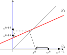
Figure 1: Illustration of accelerated MAP for a two-set feasibility problem with union convex sets. $P_{S_{2}}$ is multivalued on the gray line.

In this section, We follow the scheme described in Algorithm 1 and the discussion on component identification in Remark 4.6 to propose two such acceleration techniques. The first one is motivated by the following example.

Example 5.15.

Let $\mathbb{E}={\rm I}\!{\rm R}^{2}$, $S_{1}$ be any straight line with a positive slope, and $S_{2}=A\cup B$, where $A\coloneqq\{(a,0):a\geq 0\},B\coloneqq\{(0,b):b\geq 0\}$; see Fig. 1. Consider Eq. OP with $f(w)=\frac{1}{2}\operatorname*{dist}(w,S_{1})^{2}$, $g(w)=\delta_{S_{2}}=\min\{\delta_{A}(w),\delta_{B}(w)\}$, and $h\equiv 0.$ Then it can be shown that the PDMC iterates with stepsize $\lambda=1$ coincide with the MAP iterates; see also Section 5.3.3. Notice that this algorithm generates points confined in the union convex set $S_{2}$. To speed up the convergence of the algorithm to the solution, we conduct extrapolation if two consecutive iterates lie on the same convex set. As illustrated in Fig. 1, if $w^{k-1}$ and $w^{k}$ both lie on $A$ or $B$, we extrapolate along the direction $w^{k}-w^{k-1}$ to get an intermediate point $z^{k}$ before conducting alternating projections to obtain $w^{k+1}$. Intuitively, the iterates generated by this procedure tend to get closer to $S_{1}$ faster than when (non-accelerated) MAP only is used.

Inspired by the above example, we propose to proceed with the extrapolation step in Step 1 of Algorithm 1 only when two consecutive iterates “activate” the same components in $f$, $g$ and $h$. Formally, let

$$\hat{\mathcal{D}}\coloneqq\{D_{i}(f)\cap D_{j}(g)\cap D_{m}(h):(i,j,m)\in I\times J\times M\}$$ (5.25)

and define

$$\chi_{k}\coloneqq\begin{cases}1&\text{if}~{}\phi_{\hat{\mathcal{D}}}(w^{k})\cap\phi_{\hat{\mathcal{D}}}(w^{k-1})\neq\emptyset\text{ and}~{}k\geq 1,\\ 0&\text{otherwise},\end{cases}$$ (5.26)

where $\phi_{\hat{\mathcal{D}}}$ is defined in Eq. 3.1. Then, as summarized in Algorithm 2, we simply replace the step $p_{k}$ in Step 1 of Algorithm 1 by $\chi_{k}p_{k}$ to take into account the described restriction. It is clear that global subsequential convergence of Algorithm 2 to a fixed point of $T_{\rm PDMC}^{\lambda}$ directly follows from Theorem 4.2.

Let $V=f+g-h$. Choose $\sigma>0$, $\lambda\in(0,1/L]\cap(0,\bar{\lambda})$, and $w^{0}\in\mathbb{E}$. Set $w^{-1}=w^{0}$ and $k=0$.

Step 1.

Set $z^{k}=w^{k}+t_{k}p^{k}$, where $p^{k}=\chi_{k}(w^{k}-w^{k-1})$, $\chi_{k}$ is given by Eq. 5.26, and $t_{k}\geq 0$ satisfies Eq. 4.2.

Step 2.

Set $w^{k+1}\in T_{\rm PDMC}^{\lambda}(z^{k})$, $k=k+1$, and go back to Step 1.

Algorithm 2 Accelerated PDMC algorithm for Eq. OP.

In the same spirit as Remark 4.6, applying Lemma 4.5 to Eq. 5.25 suggests that latter iterates of the Eq. PDMC algorithm indicate which components of the objective function are activated by a fixed point. Using this observation, we propose to identify and safeguard the activated component by checking consecutive component changes in Algorithm 3. Our algorithm has a spirit similar to the heuristics for manifold identification in [Li et al., 2020, Lee, 2023, Lee and Wright, 2012] but is with theoretical tools thoroughly different from these works.

Choose $w^{0}\in\mathbb{E}$, $N\in\mathbb{N}$. Set Unchanged $=0$, $k=0$.

Step 1.

Set Unchanged $=$ $\chi_{k}$(Unchanged + 1), where $\chi_{k}$ is given by Eq. 5.26.

Step 2.

Compute $w^{k+1}$ according to the following rules:

• If Unchanged $<N$: set $w^{k+1}\in T_{\rm PDMC}^{\lambda}(w^{k})$.

• If Unchanged $=N$: set Unchanged = $-1$, pick $(i,j,m)\in\phi_{\hat{\mathcal{D}}}(w^{k})$, and solve

  $$w^{k+1}\in\operatorname*{arg\,min}_{z\in\mathbb{E}}f_{i}(z)+g_{j}(z)-h_{m}(z).$$

Step 3.

Terminate if $w^{k+1}=w^{k}$; otherwise set $k=k+1$ and go back to Step 1.

Algorithm 3 PDMC with component identification for Eq. OP.

6 Affine-union convex set feasibility problems

In this section, we establish global convergence of several algorithms for solving Eq. FP involving an affine set

$$S_{1}=\{w\in{\rm I}\!{\rm R}^{q}:Aw=b\},$$ (6.1)

where $A\in{\rm I}\!{\rm R}^{m\times q}$ is a matrix with full row rank, and a union convex set $S_{2}$. Specifically, we consider the sparse affine feasibility problem and a feasibility reformulation of the linear complementarity problem in Sections 6.1 and 6.2, respectively. The results for LCPs are then applicable to GAVE following Alcantara et al. [2023] as discussed in (V) of Section 1.2. Recall that in general, the feasibility problem Eq. FP can be reformulated as an optimization problem, either as Eq. 5.13 or Eq. 5.18. Other than these reformulations, the affine structure of $S_{1}$ given by Eq. 6.1 enables recasting the feasibility problem as

$$\min_{w\in\mathbb{E}}\, \frac{1}{2}\|Aw-b\|^{2}+\frac{1}{2}\operatorname*{dist}(w,S_{2})^{2},\quad\text{ or }$$ (6.2)

$$\min_{w\in\mathbb{E}}\, \frac{1}{2}\|Aw-b\|^{2}+\delta_{S_{2}}(w).$$ (6.3)

To unify the analyses of algorithms for these four optimization reformulations, we first note that the projection onto $S_{1}$ is given by $P_{S_{1}}(w)=w-A^{\dagger}(Aw-b)$ [Bauschke and Kruk, 2004, Lemma 4.1], where, $A^{\dagger}$ is the Moore-Penrose inverse of $A$, given by $A^{\dagger}=A^{\mathsf{T}}(AA^{\mathsf{T}})^{-1}$ since $A$ has full row rank. With this, we have

$$\operatorname*{dist}(w,S_{1})^{2}=\|A^{\dagger}(Aw-b)\|^{2}=w^{\mathsf{T}}A^{\mathsf{T}}\hat{Q}Aw-2w^{\mathsf{T}}A^{\mathsf{T}}\hat{Q}b+b^{\mathsf{T}}\hat{Q}b,$$

where $\hat{Q}\coloneqq(AA^{\mathsf{T}})^{-1}$. By denoting

$$f_{Q}(w)\coloneqq\frac{1}{2}w^{\mathsf{T}}A^{\mathsf{T}}QAw-w^{\mathsf{T}}A^{\mathsf{T}}Qb+\frac{1}{2}b^{\mathsf{T}}Qb,$$ (6.4)

we get $f_{Q}(w)=\|Aw-b\|^{2}/2$ if $Q=I$, and $f_{Q}(w)=\operatorname*{dist}(w,S_{1})^{2}/2$ if $Q=(AA^{\mathsf{T}})^{-1}$. Thus, we may unify the convergence analyses of algorithms for Eqs. 5.13 and 6.2 through varying $Q$ in

$$\min_{w\in{\rm I}\!{\rm R}^{n}}f_{Q}(w)+\frac{1}{2}\operatorname*{dist}(w,S_{2})^{2},$$ (6.5)

and similarly for Eqs. 5.18 and 6.3, we may consider

$$\min_{w\in{\rm I}\!{\rm R}^{n}}f_{Q}(w)+\delta_{S_{2}}(w).$$ (6.6)

Note that $f_{Q}$ is a convex function with gradient

$$\nabla f_{Q}(w)=A^{\mathsf{T}}Q(Aw-b),$$ (6.7)

which is Lipschitz continuous with parameter

$$L_{Q}=\begin{cases}1&\text{if}~{}Q=(AA^{\mathsf{T}})^{-1},\\ \|A\|^{2}&\text{if}~{}Q=I.\end{cases}$$ (6.8)

Moreover, we have the following:

1. As noted in Section 5.3.1, $g$ and $h$ given in Eq. 5.15 satisfy Assumption 5.2 (c) and (d) since $S_{2}$ is a union convex set. By using this decomposition in Eq. 6.5 and then applying Eq. PDMC, we get

   $$T_{\rm PDMC}^{\lambda}(w^{k})=\frac{1}{1+\lambda}\left(w^{k}-\lambda\nabla f_{Q}(w)+\lambda P_{S_{2}}(w^{k})\right).$$ (6.9)

2. A direct application of Eq. FB to Eq. 6.5 with $g=\operatorname*{dist}(\cdot,S_{2})^{2}/2$ leads to

   $$T_{\rm FB}^{\lambda}(w^{k})=\frac{\lambda}{1+\lambda}P_{S_{2}}(w^{k}-\lambda\nabla f_{Q}(w^{k}))+\frac{1}{1+\lambda}(w^{k}-\lambda\nabla f_{Q}(w^{k})).$$ (6.10)

3. The PS algorithm Eq. PS for solving Eq. 6.6 is given by

   $$T_{\rm PS}^{\lambda}(w^{k})=P_{S_{2}}(w^{k}-\lambda\nabla f_{Q}(w^{k})).$$ (6.11)

When $Q=(AA^{\mathsf{T}})^{-1}$, the operators $T_{\rm PDMC}^{\lambda}$, $T_{\rm FB}^{\lambda}$ and $T_{\rm PS}^{\lambda}$ above respectively coincide with $T_{\rm MAveP}^{\lambda}$, $T_{\rm MARP}^{\lambda}$ and $T_{\rm MAP}^{\lambda}$ presented in Section 5.3.

Remark 6.1.

Except for Assumption 5.2 (e), all the other assumptions are satisfied. Together with the convexity of $f_{Q}$ and Remark 5.8 (a), we obtain from Theorem 5.7 that the algorithms Eqs. 6.9, 6.10 and 6.11 are globally convergent to fixed points if we can show that the objective functions are coercive.

6.1 Sparse affine feasibility

We consider the sparse affine feasibility problem (SAFP), which involves solving Eq. FP with Eq. 1.2, where $0<s\leq n$, $A\in{\rm I}\!{\rm R}^{m\times n}$ has full row rank and $b\in{\rm I}\!{\rm R}^{m}$. Hesse et al. [2014] have shown that $S_{2}=A_{s}$ can be decomposed as

$$A_{s}=\bigcup_{\iota\in\mathcal{I}_{s}}R_{\iota},\quad\mathcal{I}_{s}\coloneqq\{\iota\subset[n]:\iota\text{ has }s~{}\text{elements}\},\quad R_{\iota}\coloneqq\operatorname*{Ran}\left(I_{:,\iota}\right),$$ (6.12)

so $S_{2}$ is indeed a union convex set and the projection onto $S_{2}$ is given by

$$P_{S_{2}}(w)=\{P_{R_{\iota}}(w):\iota\in\mathcal{I}_{s}\text{ such that }\min_{j\in\iota}|w_{j}|\geq\max_{j\in\iota^{c}}|w_{j}|\}.$$

In turn, we can use the algorithms Eqs. 6.9 to 6.11 to solve the sparse affine feasibility problem.

We now show that these algorithms are globally convergent under conditions significantly weaker than those used in prior works Beck and Teboulle [2011], Hesse et al. [2014]. To establish our convergence results, we note the following simple but useful lemma.

Lemma 6.2.

Let $A\in{\rm I}\!{\rm R}^{m\times n}$ and $Q\in{\rm I}\!{\rm R}^{m\times m}$ be with $\operatorname*{rank}(A)=\operatorname*{rank}(Q)=m$, and let $\Lambda\subset[n]$. If $\operatorname*{rank}(A_{:,\Lambda})=\lvert\Lambda\rvert$, then $\operatorname*{rank}((A^{\mathsf{T}}QA)_{:,\Lambda})=\lvert\Lambda\rvert$. Consequently, $\lambda_{\min}((A^{\mathsf{T}}QA)_{:,\Lambda}^{\mathsf{T}}(A^{\mathsf{T}}QA)_{:,\Lambda})>0$.

Proof.

Let $E=I_{:,\Lambda}$, then $A_{:,\Lambda}=AE$ and $(A^{\mathsf{T}}QA)_{:,\Lambda}=A^{\mathsf{T}}QAE$. With the rank assumptions, the result immediately follows. ∎

Theorem 6.3.

Consider Eq. FP with Eq. 1.2. Let $A\in{\rm I}\!{\rm R}^{m\times n}$ be of full row rank, $Q\in\{(AA^{\mathsf{T}}),I\}$, and $f_{Q}$ and $L_{Q}$ be given by Eq. 6.4 and Eq. 6.8, respectively. Suppose there exists $\nu_{s}>0$ such that

$$\nu_{s}\|w\|^{2}\leq\|Aw\|^{2},\quad\forall w\in A_{s}.$$ (6.13)

Then any sequence $\{w^{k}\}$ generated by the PDMC algorithm Eq. 6.9 with $\lambda\in(0,1/L_{Q}]$ has an accumulation point $w^{*}\in\operatorname*{Fix}(T_{\rm PDMC}^{\lambda})$, and full sequence convergence holds if $T_{\rm PDMC}^{\lambda}$ is single-valued at $w^{*}$. The same conclusion holds for a sequence generated by the FB algorithm Eq. 6.10 with stepsizes $\lambda\in(0,1/L_{Q})$.

Proof.

Using Theorem 5.7, it suffices to prove that $V_{\iota}\coloneqq f_{Q}+\operatorname*{dist}(\cdot,R_{\iota})^{2}/2$ is coercive for all $\iota\in\mathcal{I}_{s}$. That is, given any $\{w^{k}\}$ such that $\|w^{k}\|\to\infty$, we need to show that $V_{\iota}(w^{k})\to\infty$. Suppose otherwise, then $\{V_{\iota}(w^{k})\}$ must have a bounded subsequence, and we assume without loss of generality that the whole sequence is bounded. Since

$$V_{\iota}(w^{k})=f_{Q}(w^{k})+\frac{1}{2}\|w^{k}-P_{R_{\iota}}(w^{k})\|^{2}=f_{Q}(w^{k})+\frac{1}{2}\|(w^{k})_{\iota^{c}}\|^{2},$$ (6.14)

$\{(w^{k})_{\iota^{c}}\}$ must be bounded, and hence $\|(w^{k})_{\iota}\|\to\infty$ since we are given that $\|w^{k}\|\to\infty$. Meanwhile, for $Q=(AA^{\mathsf{T}})^{-1}$, we have

$$f_{Q}(w^{k}) =\frac{1}{2}\|(A^{\dagger}A)_{:,\iota}(w^{k})_{\iota}+(A^{\dagger}A)_{:,\iota^{c}}(w^{k})_{\iota^{c}}-A^{\dagger}b\|^{2}$$

$$\geq\frac{1}{2}\lambda_{\min}\left((A^{\dagger}A)_{:,\iota}^{\mathsf{T}}(A^{\dagger}A)_{:,\iota}\right)\|(w^{k})_{\iota}\|^{2}+\frac{1}{2}\|(A^{\dagger}A)_{:,\iota^{c}}(w^{k})_{\iota^{c}}-A^{\dagger}b\|^{2}$$

$$\quad-\|(A^{\dagger}A)_{:,\iota}\|\cdot\|(w^{k})_{\iota}\|\cdot\|(A^{\dagger}A)_{:,\iota^{c}}(w^{k})_{\iota^{c}}-A^{\dagger}b\|$$ (6.15)

On the other hand, if $Q=I$, we obtain by a similar computation that

$$f_{Q}(w^{k})\geq\frac{1}{2}\lambda_{\min}(A_{:,\iota}^{\mathsf{T}}A_{:,\iota})\|(w^{k})_{\iota}\|^{2}+\frac{1}{2}\|A_{:,\iota^{c}}(w^{k})_{\iota^{c}}-b\|^{2}-\|A_{:,\iota}\|\cdot\|(w^{k})_{\iota}\|\cdot\|A_{:,\iota^{c}}(w^{k})_{\iota^{c}}-b\|.$$ (6.16)

By Eq. 6.13, it is clear that $\operatorname*{rank}(A_{:,\iota})=\lvert\iota\rvert$. Thus, by Lemma 6.2, $\lambda_{\min}\left((A^{\dagger}A)_{:,\iota}^{\mathsf{T}}(A^{\dagger}A)_{:,\iota}\right)>0$ and $\lambda_{\min}(A_{:,\iota}^{\mathsf{T}}A_{:,\iota})>0$. Letting $k\to\infty$ in Eq. 6.15 and Eq. 6.16, we then obtain that $f_{Q}(w^{k})\to\infty$, and so by Eq. 6.14, $V_{\iota}(w^{k})\to\infty$, which is a contradiction. Hence, $V_{\iota}$ is coercive, as desired. ∎

We now show $Q$-linear convergence of the PS algorithm for solving Eq. 6.6.

Theorem 6.4.

Consider the setting of Theorem 6.3. Then any sequence $\{w^{k}\}$ generated by Eq. 6.11 with $\lambda\in(0,1/L_{Q})$ has an accumulation point $w^{*}\in\operatorname*{Fix}(T_{\rm PS}^{\lambda})$, and if $T_{\rm PS}^{\lambda}$ is single-valued at $w^{*}$, then the algorithm converges to $w^{*}$ at a local $Q$-linear rate.

Proof.

Given any $\iota\in\mathcal{I}_{s}$ and any sequence $\{w^{k}\}$ that lies in $R_{\iota}$ such that $\|w^{k}\|\to\infty$, clearly $(w^{k})_{\iota^{c}}=0$ for all $k$. Consequently, by noting that $\lambda_{\min}\left((A^{\dagger}A)_{:,\iota}^{\mathsf{T}}(A^{\dagger}A)_{:,\iota}\right)$ and $\lambda_{\min}\left((A^{\mathsf{T}}A)_{:,\iota}^{\mathsf{T}}(A^{\mathsf{T}}A)_{:,\iota}\right)$ are both strictly positive from the proof of Theorem 6.3, we obtain from Eqs. 6.15 and 6.16 that $f_{Q}(w^{k})\to\infty$. Thus, $f_{Q}$ is coercive over $R_{\iota}$, showing that Assumption 5.2 (e) is fulfilled. To complete the proof, by Proposition 5.9, it suffices to show that $Id-\lambda\nabla f_{Q}$ is a contraction over $R_{\iota}$. Suppose that $Q=(AA^{\mathsf{T}})^{-1}$ and $w,w^{\prime}\in R_{\iota}$, then

$$\|\nabla f_{Q}(w)-\nabla f_{Q}(w^{\prime})\|^{2} =\|(A^{\dagger}A)_{:,\iota}(w-w^{\prime})_{\iota}\|^{2}$$

$$\geq\lambda_{\min}\left((A^{\dagger}A)_{:,\iota}^{\mathsf{T}}(A^{\dagger}A)_{:,\iota}\right)\|(w-w^{\prime})_{\iota}\|^{2}$$

$$=\lambda_{\min}\left((A^{\dagger}A)_{:,\iota}^{\mathsf{T}}(A^{\dagger}A)_{:,\iota}\right)\|w-w^{\prime}\|^{2}.$$ (6.17)

Similarly, for $Q=I$ and $w,w^{\prime}\in R_{\iota}$, we have

$$\|\nabla f_{Q}(w)-\nabla f_{Q}(w^{\prime})\|^{2}\geq\lambda_{\min}\left((A^{\mathsf{T}}A)_{:,\iota}^{\mathsf{T}}(A^{\mathsf{T}}A)_{:,\iota}\right)\|w-w^{\prime}\|^{2}.$$ (6.18)

By Eq. 6.8 and the Lipschitz continuity of $\nabla f_{Q}$, Eqs. 6.17 and 6.18 further lead to

$$\|\left(w-\lambda\nabla f(w)\right)-\left(w^{\prime}-\lambda\nabla f(w^{\prime})\right)\|\leq\kappa_{\iota}\|w-w^{\prime}\|,\quad\forall w,w^{\prime}\in R_{\iota},$$

where

$$\kappa_{\iota}^{2}=\begin{cases}1+(\lambda^{2}-2\lambda)\lambda_{\min}\left((A^{\dagger}A)_{:,\iota}^{\mathsf{T}}(A^{\dagger}A)_{:,\iota}\right)&\text{if }Q=(AA^{\mathsf{T}})^{-1},\\ 1+(\lambda^{2}-2\lambda\|A\|^{-2})\lambda_{\min}\left((A^{\mathsf{T}}A)_{:,\iota}^{\mathsf{T}}(A^{\mathsf{T}},A)_{:,\iota}\right)&\text{if }Q=I.\end{cases}$$

Since the second term is negative for $\lambda\in(0,1/L_{Q})$, $\kappa_{\iota}\in[0,1)$ and the conclusion follows. ∎

6.2 Linear complementarity problems and general absolute value equations

We now turn our attention to the linear complementarity problem (LCP) described in Eq. 1.3 and consider the feasibility problem reformulation Eq. FP with Eq. 1.4. We note that $A$ given in Eq. 1.4 has full row rank for any matrix $M$. Observe that $S_{1}$ is an affine set and $S_{2}$ also has a sparsity structure such that $S_{2}\subset A_{n}$. However, $S_{2}$ has additional properties that distinguishes it from $A_{n}$, including the nonnegativity of its vectors as well as the complementarity between $(w_{1},\dots,w_{n})$ and $(w_{n+1},\dots,w_{2n})$.

As shown in [Alcantara et al., 2023, Proposition 2.2], $z\in P_{S_{2}}(w)$ if and only if

$$(z_{j},z_{n+j})\in\begin{cases}\{(0,(w_{n+j})_{+})\}&\text{if}~{}w_{j}<w_{n+j},\\ \{((w_{j})_{+},0)\}&\text{if}~{}w_{j}>w_{n+j},\\ \{(0,(w_{n+j})_{+}),((w_{j})_{+},0)\}&\text{if}~{}w_{j}=w_{n+j},\\ \end{cases}\quad\forall j\in[n].$$

We also get from [Alcantara et al., 2023, Section 3.1] that $S_{2}$ can be decomposed as a union of closed convex sets:

$$S_{2}=\bigcup_{\iota\in\mathcal{I}}R_{\iota},\quad\text{ where }R_{\iota}\coloneqq\operatorname*{Ran}(I_{:,\iota})\cap{\rm I}\!{\rm R}^{2n}_{+},$$ (6.19)

where ${\rm I}\!{\rm R}^{2n}_{+}$ denotes the set of nonnegative vectors in ${\rm I}\!{\rm R}^{2n}$, and $\mathcal{I}$ is the set of all $\iota\subset[2n]$ expressible as $\iota=\Lambda_{1}\cup\Lambda_{2}$ for some $\Lambda_{1}\subset[n]$ and $\Lambda_{2}=\{n+j:j\in[n],j\notin\Lambda_{1}\}$. It is also clear that for any $\iota\in\mathcal{I}$ and $w\in{\rm I}\!{\rm R}^{2n}$, the projection $z$ of $w$ onto $R_{\iota}$ is given by

$$(z_{j},z_{n+j})=\begin{cases}((w_{j})_{+},0)&\text{if}~{}j\in\iota\\ (0,(w_{n+j})_{+})&\text{if}~{}j\notin\iota\end{cases},\quad\forall j\in[n].$$ (6.20)

6.2.1 LCPs involving nondegenerate and $P$-matrices

In Section 6.1, the condition Eq. 6.13 relaxed from SRIP was used to establish the convergence of the algorithms Eqs. 6.9 to 6.11. For the feasibility reformulation of LCP, a property similar to Eq. 6.13 can be obtained through assumptions on $M$ that are conventional in the LCP literature.

Definition 6.5.

A matrix $M\in{\rm I}\!{\rm R}^{n\times n}$ is said to be nondegenerate if all of its principal minors are nonzero.

Lemma 6.6.

Let $M\in{\rm I}\!{\rm R}^{n\times n}$ be a nondegenerate matrix, and $A=\begin{bmatrix}M&-I\end{bmatrix}$. Then for $S_{2}$ given by Eq. 1.4, there exists $\nu>0$ such that

$$\nu\|w\|^{2}\leq\|Aw\|^{2},\quad\forall w\in S_{2}\cup(-S_{2}).$$

Proof.

If $\iota\in\mathcal{I}$ and $w\in R_{\iota}\cup(-R_{\iota})$,

$$\|Aw\|^{2}=\|A_{:,\iota}w_{\iota}\|^{2}\geq\lambda_{\min}(A_{:,\iota}^{\mathsf{T}}A_{:,\iota})\|w_{\iota}\|^{2}=\lambda_{\min}(A_{:,\iota}^{\mathsf{T}}A_{:,\iota})\|w\|^{2}=\nu_{\iota}\|w\|^{2},$$

where $\nu_{\iota}=\lambda_{\min}(A_{:,\iota}^{\mathsf{T}}A_{:,\iota})$. Meanwhile, nondegeneracy of $M$ implies that the square matrix $A_{:,\iota}$ is nonsingular by [Alcantara et al., 2023, Lemma 2.10], so $\nu_{\iota}>0$. By taking $\nu=\min_{\iota\in\mathcal{I}}\nu_{\iota}$ and noting Eq. 6.19, we get the desired inequality. ∎

With the above lemma, we can easily obtain convergence for Eqs. 6.9, 6.10 and 6.11 on the feasibility reformulation of LCPs.

Theorem 6.7.

Let $M\in{\rm I}\!{\rm R}^{n\times n}$ be a nondegenerate matrix, $b\in{\rm I}\!{\rm R}^{n}$, $A=\begin{bmatrix}M&-I\end{bmatrix}$, $Q\in\{(AA^{\mathsf{T}})^{-1},I\}$, and $f_{Q}$ and $L_{Q}$ be given by Eq. 6.4 and Eq. 6.8, respectively, then for Eq. FP with Eq. 1.4:

1. Any sequence $\{w^{k}\}$ generated by Eq. 6.9 with $\lambda\in(0,1/L_{Q}]$ has an accumulation point $w^{*}\in\operatorname*{Fix}(T_{\rm PDMC}^{\lambda})$, and full sequence convergence holds if $T_{\rm PDMC}^{\lambda}$ is single-valued at $w^{*}$.

2. Any sequence $\{w^{k}\}$ generated by Eq. 6.10 with $\lambda\in(0,1/L_{Q})$ has an accumulation point $w^{*}\in\operatorname*{Fix}(T_{\rm FB}^{\lambda})$, and full sequence convergence holds if $T_{\rm FB}^{\lambda}$ is single-valued at $w^{*}$.

3. Any sequence $\{w^{k}\}$ generated by Eq. 6.11 with $\lambda\in(0,1/L_{Q})$ has an accumulation point $w^{*}\in\operatorname*{Fix}(T_{\rm PS}^{\lambda})$, and full sequence convergence holds if $T_{\rm PS}^{\lambda}$ is single-valued at $w^{*}$. Moreover, the convergence rate is locally linear.

Proof.

Let $\iota\in\mathcal{I}$. We define $V_{\iota}\coloneqq f_{Q}+\operatorname*{dist}(\cdot,R_{\iota})^{2}/2$, and see from Eq. 6.20 that

$$V_{\iota}(w)=f_{Q}(w)+\frac{1}{2}\|w_{\iota}-[w_{\iota}]_{+}\|^{2}+\frac{1}{2}\|w_{\iota^{c}}\|^{2}\geq f_{Q}(w)+\frac{1}{2}\|w_{\iota^{c}}\|^{2}.$$ (6.21)

Using Eq. 6.21 and Lemma 6.6, the rest of the proof follows from arguments analogous to those in the proofs of Theorems 6.3 and 6.4. ∎

For a special class of nondegenerate matrices, known as $P$-matrices, we can obtain finer results.

Definition 6.8.

A matrix $M\in{\rm I}\!{\rm R}^{n\times n}$ is said to be a $P$-matrix if all of its principal minors are positive.

It is known that Eq. 1.3 has a unique solution for any $b\in{\rm I}\!{\rm R}^{n}$ when $M$ is a $P$-matrix [Cottle et al., 1992, Theorem 3.3.7]. Consequently, $S_{1}\cap S_{2}$ contains a single point when $M$ is a $P$-matrix for $S_{1}$ and $S_{2}$ defined in Eq. 1.4. Some important applications of LCP involving $P$-matrices can be found in Schäfer [2004]. For $P$-matrices, we derive the following nice result on the characterization of fixed points. The proof of this result is quite technical and heavily relies on a special property of $P$-matrices described in Lemma A.4, and thus we defer it to Appendix B.

Theorem 6.9.

Consider the setting of Theorem 6.7. If $M$ is a $P$-matrix, then

$$\operatorname*{Fix}\left(T_{\rm PDMC}^{\lambda}\right)=\operatorname*{Fix}\left(T_{\rm FB}^{\lambda}\right)=\operatorname*{Fix}\left(T_{\rm PS}^{\lambda}\right)=S_{1}\cap S_{2},\quad\forall\lambda\in(0,1/L_{Q}].$$

Combining Theorem 6.9 and Theorem 6.7, we obtain global convergence of the algorithms to the solution set of the problem, for both the non-accelerated and the accelerated versions.

Corollary 6.10 (Global convergence to solution set).

The algorithms given in Theorem 6.7 and their accelerated versions via Algorithm 2 are globally convergent to $S_{1}\cap S_{2}$ if $M$ is a $P$-matrix. Moreover, the projected subgradient algorithm converges $Q$-linearly to $S_{1}\cap S_{2}$.

Proof.

In the proof of Theorem 6.7, we have shown the coercivity of the corresponding Lyapunov functions of the algorithms. Hence, by Eq. 4.2, Algorithm 2 generates a bounded sequence, and accumulation points are fixed points by Theorem 4.2. Together with Theorem 6.9, any sequence generated by Algorithm 2 must converge to the unique point in $S_{1}\cap S_{2}$. Setting $t_{k}\equiv 0$ in Algorithm 2 gives the desired result for the non-accelerated algorithms. Local linear convergence of the projected subgradient algorithm follow from Theorem 6.7 (c). ∎

Remark 6.11.

In the same spirit as in the discussions in Remark 4.6, Remark 5.8 (b), and Section 5.5, we note that latter iterations of the algorithms Eqs. 6.9, 6.10 and 6.11 indicate which $\iota\in\mathcal{I}$ can be used to reduce the original problems Eqs. 6.5 and 6.6 into the simpler problem of finding a point in $S_{1}\cap R_{\iota}$. For the LCP, finding $S_{1}\cap R_{\iota}$ is equivalent to solving the system $Aw^{*}=b$ and $w^{*}_{\Lambda_{\iota^{c}}}=0$, which is simply an $n\times n$ system of linear equations. If the obtained solution satisfies $w^{*}_{\iota}\geq 0$, then $w^{*}$ is indeed a solution of the original feasibility problem. For Eqs. 6.9, 6.10 and 6.11 and their extrapolation-accelerated versions by Algorithm 2, Corollary 6.10 guarantees that these algorithms will converge to the unique point $w^{*}$ in $S_{1}\cap S_{2}$ when $M$ is a $P$-matrix. Thus, theoretically, we know that Algorithm 3 will indeed output the solution $w^{*}$. Similarly, for the sparse affine feasibility problem, the reduced feasibility problem of finding a point in $S_{1}\cap R_{\iota}$ amounts to solving the linear system $A_{:,\iota}w_{\iota}=b$. These remarks will be used in the numerical implementation of Algorithm 3 in Section 7.

6.2.2 Special properties of the projected subgradient algorithm for LCP

We already know from Corollary 6.10 that the projected subgradient algorithm Eq. 6.11 is globally convergent to $S_{1}\cap S_{2}$ for stepsizes $\lambda\in(0,1/L_{Q})$. In this section, we show that the result also holds for $\lambda=1/L_{Q}$. This in turn shows the global convergence of the method of alternating projections by setting $Q=(AA^{\mathsf{T}})^{-1}$, which is a rare result in the nonconvex setting. Indeed, proving such a result for the LCP requires a number of technical lemmas, an indication that global convergence for MAP is indeed difficult to obtain for nonconvex problems in general.

In addition to Theorem 6.9, the following proposition is needed for proving the desired global convergence result. As the proof needs many other technical lemmas, we defer its presentation to Appendix A.

Theorem 6.12.

Consider the setting of Theorem 6.7. Let $w\in S_{2}\setminus\operatorname*{Fix}(T_{\rm PS}^{\lambda})$ and $w^{+}\in T_{\rm PS}^{\lambda}(w)$ where $\lambda\in(0,1/L_{Q}]$. If $M$ is a $P$-matrix, then $f_{Q}(w^{+})<f_{Q}(w)$. Consequently, $V\coloneqq f_{Q}+\delta_{S_{2}}$ is a Lyapunov function for Eq. PS for any $\lambda\in(0,1/L_{Q}]$.

We now state our main result showing the convergence of Eq. 6.11 with stepsize $\lambda=1/L_{Q}$. We highlight that for a sequence generated by the PS algorithm, we obtain an additional property that the objective function values $\{f_{Q}(w^{k})\}$ decreases to zero $Q$-linearly as well.

Theorem 6.13.

Let $M$ be a $P$-matrix, $b\in{\rm I}\!{\rm R}^{n}$, $A=[M~{}-I]$, and consider Eq. FP with Eq. 1.4. Denote by $w^{*}$ the unique point in $S_{1}\cap S_{2}$ and let $Q\in\{(AA^{\mathsf{T}})^{-1},I\}$, and $f_{Q}$ and $L_{Q}$ be given by Eq. 6.4 and Eq. 6.8, respectively. Any sequence generated by Eq. 6.11 with $\lambda\in(0,1/L_{Q}]$ converges to $w^{*}$ with a local $Q$-linear rate. Moreover, the objective function Eq. 6.6 converges to the global optimum of $0$ with a local $Q$-linear rate.

Proof.

Linear convergence of $\{w^{k}\}$ to $w^{*}$ when $\lambda\in(0,1/L_{Q})$ is already provided in Theorem 6.7. Linear convergence for $\lambda=1/L_{Q}$ can be proved using the fact from Theorem 6.12 that $V=f_{Q}+\delta_{S_{2}}$ is a Lyapunov function when $\lambda=1/L_{Q}$, together with Remark 5.5, Theorem 6.9, and the techniques used in Theorem 6.7. Thus, it remains to show that $f_{Q}(w^{k})\to 0$ at a $Q$-linear rate.

From Remark 5.8 (b), we know that there exists $N\geq 0$ such that $w^{k}\in R_{\iota}$ for all $k\geq N$ and for any $\iota\in\mathcal{I}$ such that $w^{*}\in R_{\iota}$. It then follows that $w^{k}-w^{*}\in S_{2}\cup(-S_{2})$ for all $k\geq N$. Suppose now that $Q=(AA^{\mathsf{T}})^{-1}$. By using Lemma 6.6 and noting that $AA^{\dagger}=I$, we get

$$\nu\|w^{k}-w^{*}\|^{2}\leq\|A(w^{k}-w^{*})\|^{2}=\|(AA^{\dagger})A(w^{k}-w^{*})\|^{2}\leq\|A\|^{2}\cdot\|A^{\dagger}A(w^{k}-w^{*})\|^{2},$$

that is,

$$\frac{\nu}{\|A\|^{2}}\|w^{k}-w^{*}\|^{2}\leq\|A^{\dagger}A(w^{k}-w^{*})\|^{2},\quad\forall k\geq N.$$ (6.22)

On the other hand, if $Q=I$, we immediately get from Lemma 6.6 that

$$\nu\|w^{k}-w^{*}\|^{2}\leq\|A(w^{k}-w^{*})\|^{2},\quad\forall k\geq N.$$ (6.23)

Since $w^{*}\in S_{1}$, with Eqs. 6.22 and 6.23, we obtain that

$$\frac{1}{2}\|w^{k}-w^{*}\|^{2}\leq\eta f_{Q}(w^{k}),\,\forall k\geq N,\,\text{where}\,\eta=\begin{cases}\frac{\|A\|^{2}}{\nu}&\text{if}~{}Q=(AA^{\mathsf{T}})^{-1}\\ \frac{1}{\nu}&\text{if}~{}Q=I.\end{cases}$$ (6.24)

Then,

$$f_{Q}\left(w^{k+1}\right) \overset{\lx@cref{creftype~refnum}{eq:f<=Qf}}{\leq}\min_{z\in S_{2}}\;Q_{f_{Q}}^{\lambda}(z,w^{k})$$

$$\leq\min_{\alpha\in[0,1]}\;f_{Q}\left(\alpha w^{*}+(1-\alpha)w^{k}\right)+\frac{1}{2\lambda}\left\|w^{k}-\left(\alpha w^{*}+(1-\alpha)w^{k}\right)\right\|^{2}$$

$$\leq(1-\alpha)f_{Q}(w^{k})+\frac{\alpha^{2}}{2\lambda}\left\|w^{k}-w^{*}\right\|^{2},\quad\forall\alpha\in[0,1],$$

where the last inequality is from the convexity of $f_{Q}$ and the fact that $f_{Q}(w^{*})=0$. Applying Eq. 6.24 to the inequality above then gives

$$f_{Q}\left(w^{k+1}\right)\leq\left(1-\alpha+\frac{\eta}{\lambda}\alpha^{2}\right)f_{Q}(w^{k}),\quad\forall\alpha\in[0,1].$$ (6.25)

The claim now follows by minimizing the right-hand side of Eq. 6.25 with respect to $\alpha$. ∎

7 Numerical experiments

This section presents numerical experiments on sparse affine feasibility and linear complementarity problems to support the established theoretical convergence of the proposed algorithms and to demonstrate the efficiency of the acceleration schemes Algorithms 2 and 3. For simplicity, we focus on the projected gradient algorithm Eq. 6.11 with $Q\in\{I_{n},(AA^{\mathsf{T}})^{-1}\}$. We keep the notations PS for $Q=I$ and MAP for $Q=(AA^{\mathsf{T}})^{-1}$. We include a prefix “A” and/or a suffix “$+$” to signify that Algorithm 2 and/or Algorithm 3 are incorporated in the algorithms. All experiments are conducted on a machine running Ubuntu 20.04 and MATLAB R2021b with 64GB memory and an Intel Xeon Silver 4208 CPU with 8 cores and 2.1 GHz. To satisfy Eq. 4.2 in Algorithm 2, since $f_{Q}$ is a quadratic function, a closed form stepsize is obtained by taking $t_{k}=\max\{0,\min\{t_{k}^{(1)},t_{k}^{(2)}\}\}$ for the LCP and $t_{k}=\max\{0,t_{k}^{(1)}\}$ for the SAFP, where $t_{k}^{(1)}=\frac{-2\nabla f_{Q}(w^{k})^{\mathsf{T}}p^{k}}{(Ap^{k})^{\mathsf{T}}Q(Ap^{k})+\sigma\|p^{k}\|^{2}}$ and $t_{k}^{(2)}=\min\{-w_{j}^{k}/p_{j}^{k}:p_{j}^{k}<0\}$.

7.1 Sparse affine feasibility problem

We consider SAFP with synthetic and real datasets described below and compare our methods with the proximal gradient method by Beck and Teboulle [2011], which we denote by PG-BT. For PS/MAP, we set $\lambda=\tau/L_{Q}$ with $\tau=0.999$ (see Theorem 6.4) and $\sigma=10^{-2}$. The parameter $N$ in Algorithm 3 is set to $50$ for MAP and $100$ for PS. When Algorithm 3 is used in combination with Algorithm 2, we set $N$ to half its specified value when only Algorithm 3 is used. The linear system described in Remark 6.11 for dealing with Step 2.2 of Algorithm 3 is handled by solving $A_{:,\iota}^{\top}A_{:,\iota}w_{\iota}=A_{:,\iota}^{\top}b$ using the conjugate gradient (CG) method (see, for example, [Nocedal and Wright, 2006, Chapter 5]). For the SAFP problems, the cost of one CG iteration is $O(ms)$ and the number of CG iterations in one round of Step 2.2 of Algorithm 3 is upper bounded by $s$. Hence, the overall cost of invoking the CG procedure once is at most $O(ms^{2})$, although we often observe that CG terminates within few iterations in practice, while one step of Eq. 6.11 is $O(mn)$. We also observe that empirically the CG procedure takes an almost negligible amount of running time in the whole procedure. All algorithms are initialized with $w^{0}=A^{\mathsf{T}}b$, and the residual is measured by

$$\text{Residual}\coloneqq\frac{1}{2}\|Aw^{k}-b\|^{2}+\frac{1}{2}\operatorname*{dist}(w^{k},S_{2})^{2},$$ (7.1)

which is $0$ if and only if $w^{k}$ is a solution to the SAFP.

Synthetic data. We follow Becker et al. [2011] to generate standard random test problems involving a matrix $A\in{\rm I}\!{\rm R}^{m\times n}$ with entries sampled from the standard normal distribution, and a sparse signal $w^{*}\in A_{s}$ such that the nonzero entries $w_{i}^{*}$ are generated as $w_{i}^{*}=\eta_{1}10^{\alpha\eta_{2}}$ with $\alpha=5$, $\eta_{1}=\pm 1$ with probability 0.5, and $\eta_{2}$ uniformly sampled from $[0,1]$. After generating $A$ and $w^{*}$, we set $b=Aw^{*}$ so that $w^{*}$ is a solution of the SAFP. The running time and total iterations required for reducing Eq. 7.1 below $10^{-6}$ with $n=10000$, $m=2500$, and $s=625$ over ten independent trials are summarized in Table 1.

We see from Table 1 that the acceleration schemes Algorithms 2 and 3 reduce both the running time and the number of iterations of the algorithms. The non-accelerated MAP algorithm is already more efficient than PG-BT, but when $Q=I$, only the accelerated versions of PS have better performance than PG-BT. Finally, we observe that for this experiment, Algorithm 2 has faster convergence than Algorithm 3, and incorporating component identification to Algorithm 2 only resulted to minimal improvements in convergence time. Component identification in this experiment only helped to reduce the residual to a much lower level after the stopping criterion of $10^{-6}$ is almost reached.

Table 1: Performance of algorithms on ten independent trials of SAFP with synthetic data. For the running time and residual of each method, we report their average$\pm$standard deviation. Ave. CI Iters. refers to the average number of times Step 2.2 in Algorithm 3) is executed, while Ave. CI Time is the average amount of time required to finish one CI iteration. PS and PS+ are omitted as they failed to solve the problems after 10000 iterations.

Method	Ave.	Time	Ave.	Ave.	Residual
	Iters	(seconds)	CI Iters	CI Time
MAP	673.6	10.6 $\pm$ 0.2	NA	NA	9.3e-07 $\pm$ 4.5e-08
AMAP	263.4	4.5 $\pm$ 0.3	NA	NA	7.8e-07 $\pm$ 8.6e-08
MAP+	600.1	9.5 $\pm$ 0.2	1.2	0.014	1.4e-10 $\pm$ 4.5e-11
AMAP+	250.1	4.3 $\pm$ 0.3	1	0.014	1.4e-10 $\pm$ 4.5e-11
APS	417.5	5.7 $\pm$ 0.3	NA	NA	8.4e-07 $\pm$ 6.7e-08
APS+	402.9	5.5 $\pm$ 0.3	1	0.014	1.4e-10 $\pm$ 4.5e-11
PG-BT	847.0	15.3 $\pm$ 0.6	NA	NA	9.5e-07 $\pm$ 4.2e-08

Real-world datasets. We then consider three public real-world datasets: colon-cancer ($m=62$, $n=2000$), duke breast-cancer ($m=44$, $n=7129$) and leukemia ($m=38$, $n=7129$). We set $s$ to 5% of the total number of features $n$. The results are summarized in Fig. 2.

Similar to the results on synthetic datasets, the acceleration schemes Algorithms 2 and 3 reduce both the running time and the number of iterations of the algorithms, except that component identification in Algorithm 3 did not take place for duke breast-cancer. For the other two datasets, component identification greatly reduced both the running time and the number of iterations. The algorithms corresponding to $Q=(AA^{\mathsf{T}})^{-1}$ also provided performance better than those with $Q=I$ and PG-BT.

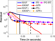
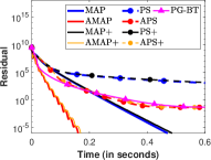
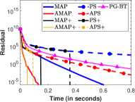
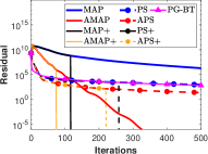
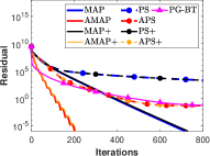
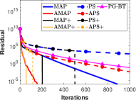
colon-cancer	duke breast-cancer	leukemia

Figure 2: Comparisons of running time and iteration number of algorithms for solving SAFP with real-world datasets.

7.2 Linear complementarity problem

We consider standard LCP test problems as follows and compare our algorithms with BPA and EGA mentioned in Section 2.

LCP1. [Qi et al., 2000, Example 2] $M$ is a tridiagonal matrix with $M_{ii}=4$ for all $i\in[n]$ and $M_{ij}=-1$ when $|i-j|=1$, and $b=(1,1,\dots,1)^{\mathsf{T}}$.

LCP2. [Kanzow, 1996, Example 7.1] $M$ is an upper triangular matrix with $M_{ii}=1$ for all $i\in[n]$, $M_{ij}=2$ for all $i<j$, and $b=(1,1,\dots,1)^{\mathsf{T}}$. BPA is excluded for this case as it is applicable only when $M+M^{\mathsf{T}}$ is positive definite [Facchinei and Pang, 2003, Theorem 12.1.2].

LCP3. [Kanzow, 1996, Example 7.3] The entries of $b$ are independently sampled from uniform random with range $(-500,500)$. $M$ is a $P$-matrix given by $M=A_{1}^{\mathsf{T}}A_{1}+A_{2}+{\rm diag}(\eta)$, where $A_{1},A_{2}\in{\rm I}\!{\rm R}^{n\times n}$ are matrices with entries independently sampled from uniform random in $(-5,5)$, $A_{2}$ is skew-symmetric, and each entry of $\eta\in{\rm I}\!{\rm R}^{n}$ is independently taken from uniform random of $(0,0.3)$.

We set $\lambda=1$ for MAP according to Theorem 6.13. $\sigma$ and $N$ follow the setting in the preceding section. Matlab’s backslash operator is used to handle the linear system described in Remark 6.11, with the cost of $O(n^{3})$ for our problem, which is of the same order as the overhead of computing $Q$ and $L_{Q}$. On the other hand, the cost of one iteration of Eq. PDMC is $O(n^{2})$. We will see in the experimental results that although component identification in this case is slightly more expensive than its counterpart in the SAFP experiment, it still takes only a small portion of the overall running time of the algorithms. We set $n=5000$ in all of the experiments, and divide both $M$ and $b$ by the same scalar $\|M\|_{1}/\sqrt{n}$. This normalization is due to the geometric observation that for $n=1$, projection algorithms tend to converge faster to a solution when the slope is in a moderate range. Instead of Eq. 7.1, we use the following standard measure of residual in LCP [Facchinei and Pang, 2003, Proposition 1.5.8] to facilitate fair comparisons with BPA and EGA.

$$\text{Residual}\coloneqq\|\min(x^{k},Mx^{k}-b)\|.$$ (7.2)

We report the running time and iterations required for reducing Eq. 7.2 below $10^{-6}$. For the feasibility reformulation of the LCP (see Section 6.2), the first $n$ coordinates of $w^{k}$ correspond to $x^{k}$.

We see from Fig. 3 and Table 2 that indeed, the proposed acceleration schemes significantly reduce the required time and number of iterations to solve the generated LCPs. The only exception is LCP1, on which the non-accelerated algorithms terminate before reaching the specified $N$ for Algorithm 3, so component identification is not executed at all. The residual of MAP+ presented in Table 2 tends to be much lower than our stopping condition, as the linear system solver is non-iterative and cannot be terminated exactly at the point where the required residual tolerance is met. On the other hand, for AMAP+, component identification does not change the residual much. A closer examination revealed that in this case, the algorithm sometimes terminates without triggering component identification.

Overall speaking, the proposed acceleration scheme in Algorithm 1 using extrapolation is indeed very effective in reducing the running time and iterations of fixed-point maps, while the component identification part in Algorithm 3 is more useful when highly accurate solutions are required.

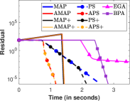
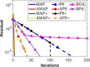
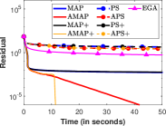
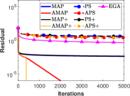
LCP1		LCP2

Figure 3: Comparisons of running time and iteration number of algorithms for solving LCP1 and LCP2. For LCP1, the algorithms MAP, AMAP and APS overlap with MAP+, AMAP+ and APS+. Comparison with BPA on LCP2 is omitted because BPA is not applicable.

Table 2: Performance of algorithms on ten independent trials of LCP3 for reducing Eq. 7.2 to below $10^{-6}$. BPA and algorithms corresponding to $Q=I$ are omitted as all of them failed to make the residual below $10^{-6}$ in 10000 iterations. Ave. CI Iters. refers to the average number of times Step 2.2 in Algorithm 3) is executed, while Ave. CI Time is the average amount of time required to finish one CI iteration.

Method	Ave.	Time	Ave.	Ave.	Residual
	Iters	(seconds)	CI Iters	CI Time
MAP	979.0	20.9 $\pm$ 1.3	NA	NA	1.0e-06 $\pm$ 2.3e-09
AMAP	244.1	6.3 $\pm$ 0.4	NA	NA	8.8e-07 $\pm$ 1.2e-07
MAP+	577.1	16.1 $\pm$ 2.1	2.8	1.2	2.2e-15 $\pm$ 1.0e-16
AMAP+	238.0	7.1 $\pm$ 0.5	0.8	1.2	1.4e-07 $\pm$ 2.9e-07
EGA	914.4	11.8 $\pm$ 0.4	NA	NA	9.9e-07 $\pm$ 7.5e-09

8 Conclusion

In this work, we analyzed the global subsequential convergence of fixed point iterations of union upper semicontinuous operators, and prove global convergence under a local Lipschitz condition. We show that this class of fixed point algorithms in fact covers several iterative methods for solving optimization and feasibility problems alike, and therefore global convergence of these methods is a consequence of the derived theory for the general setting of fixed point problems. In particular, we establish global convergence of proximal algorithms for minimizing a class of nonconvex nonsmooth functions, specifically those that can be expressed as the sum of a piecewise smooth mapping and a function that is the difference of a min-$\rho$-convex and a convex function. Linear convergence is also proven under a mild calmness condition. We also prove global convergence of traditional projection methods for solving feasibility problems involving union convex sets. Acceleration methods via extrapolation and component identification are proposed by utilizing the special structure of the defining operators of the algorithms. Numerical evidence illustrated that our proposed acceleration schemes provide significant improvement over the non-accelerated ones in terms of both the running time and the number of iterations required to solve the problems. Another interesting future work is to obtain an iteration bound for the component identification result, and then to further develop global iteration complexities of the discussed algorithms on top of the identification bound.

Appendix A Proof of Theorem 6.12

We will first develop necessary tools for separately considering different cases of $w$ and $w^{+}\in T_{\rm PS}^{\lambda}(w)$. The following lemma will be our key tool to proving the desired result.

Lemma A.1.

Consider the setting of Theorem 6.7. Let $w\in S_{2}\setminus\operatorname*{Fix}(T_{\rm PS}^{\lambda})$ and $w^{+}\in T_{\rm PS}^{\lambda}(w)$ where $\lambda\in(0,1/L_{Q}]$. If $w\in R_{\iota}$, $\hat{w}\coloneqq P_{R_{\iota}}(w-\lambda\nabla f_{Q}(w))\neq w$, then $f_{Q}(w^{+})<f_{Q}(w)$.

Proof.

From Eq. 5.9, we have

$$T_{\rm PS}^{\lambda}(w)=P_{S}(w-\lambda\nabla f_{Q}(w))=\operatorname*{arg\,min}_{z\in S_{2}}\,Q_{f_{Q}}^{\lambda}(z,w).$$ (A.1)

By the convexity of $R_{\iota}$ and the definition of $\hat{w}$, we have $\langle w-\lambda\nabla f_{Q}(w)-\hat{w},w-\hat{w}\rangle\leq 0.$ Therefore,

$$\lambda\langle\nabla f_{Q}(w),\hat{w}-w\rangle=\langle\lambda\nabla f_{Q}(w)-(w-\hat{w}),\hat{w}-w\rangle+\langle w-\hat{w},\hat{w}-w\rangle\leq-\|\hat{w}-w\|^{2}.$$

Thus, from the definition of $Q_{f_{Q}}^{\lambda}$ in Eq. 5.7,

$$Q_{f_{Q}}^{\lambda}(\hat{w},w)\leq f_{Q}(w)-\frac{1}{\lambda}\|\hat{w}-w\|^{2}+\frac{1}{2\lambda}\|\hat{w}-w\|^{2}=f_{Q}(w)-\frac{1}{2\lambda}\|\hat{w}-w\|^{2}<f_{Q}(w),$$ (A.2)

where the last inequality holds because $w\neq\hat{w}$. Further, we have from Eq. 5.7 and Eq. A.1 that $f_{Q}(w^{+})\leq Q_{f_{Q}}^{\lambda}(w^{+},w)\leq Q_{f_{Q}}^{\lambda}(\hat{w},w)$, combining which with Eq. A.2 then gives the desired result. ∎

In particular, the above lemma shows that if $w\notin\operatorname*{Fix}(T_{\rm PS}^{\lambda})$ and $w^{+}\in T_{\rm PS}^{\lambda}(w)$ belong to the same convex set $R_{\iota}$, then $f_{Q}(w^{+})<f_{Q}(w)$. In the other case, we will show that there exists some $\iota\in\mathcal{I}$ such that $w\in R_{\iota}$ and the vector $\hat{w}=P_{R_{\iota}}(w-\lambda\nabla f_{Q}(w))$ is distinct from $w$. First, we consider the instance when $w$ is a nondegenerate point of $S_{2}$.

Definition A.2 (Nondegenerate point).

Let $\{R_{\iota}\}_{\iota\in\mathcal{I}}$ be a finite collection of closed convex sets, $S=\bigcup_{j\in J}R_{j}$, and $w\in S$. We say that $w$ is a nondegenerate point of $S$ if there exists a unique $\iota\in\mathcal{I}$ such that $w\in R_{\iota}$. Otherwise, it is called a degenerate point of $S$.

Proposition A.3.

Consider the setting of Theorem 6.7 (c). Let $w\in S_{2}\setminus\operatorname*{Fix}(T_{\rm PS}^{\lambda})$ and $w^{+}\in T_{\rm PS}^{\lambda}(w)$ where $\lambda\in(0,1/L_{Q}]$. If $M$ is a nondegenerate matrix and $w$ is a nondegenerate point, then $f_{Q}(w^{+})<f_{Q}(w).$

Proof.

Let $\iota\in\mathcal{I}$ such that $w\in R_{\iota}$, and let $\hat{w}$ be as in Lemma A.1. To prove the claim, we only need to show that $w\neq\hat{w}$, and then the result follows from Lemma A.1. Suppose to the contrary that $w=\hat{w}$, that is, $w=P_{R_{\iota}}(\bar{w})$ for $\bar{w}\coloneqq w-\lambda\nabla f_{Q}(w)$. Since $w=P_{R_{\iota}}(\bar{w})$ and $(w_{j},w_{n+j})\neq(0,0)$ for all $j\in[n]$ by nondegeneracy of $w$, we have from Eq. 6.20 that $w_{j}=\bar{w}_{j}>0$ and $w_{n+j}=0$ if $j\in\iota$, and $w_{n+j}=\bar{w}_{n+j}>0$ and $w_{j}=0$ otherwise. Thus,

$$(\bar{w}_{j},\bar{w}_{n+j})-(w_{j},w_{n+j})=\begin{cases}(0,\bar{w}_{n+j})&\text{if}~{}j\in\iota,\\ (\bar{w}_{j},0)&\text{if}~{}j\notin\iota,\end{cases}\quad\forall j\in[n].$$

Hence,

$$(\bar{w}_{j}-w_{j})(\bar{w}_{n+j}-w_{n+j})=0,\quad\forall j\in[n].$$ (A.3)

Since $\bar{w}-w=-\lambda\nabla f_{Q}(w)$, we have $\bar{w}-w\in\operatorname*{Ran}(A^{\mathsf{T}})=\operatorname*{Ker}(A)^{\perp}$ from Eq. 6.7. By this together with Eq. A.3 and the nondegeneracy of $M$, we have from [Alcantara et al., 2023, Proposition 2.11] that $\bar{w}-w=0$. Consequently, we have $\nabla f_{Q}(w)=0$, and since $A$ is of full row rank, it follows from Eq. 6.7 that $Aw-b=0$. That is, $w\in S_{1}$, and in turn, we get $w\in S_{1}\cap S_{2}$. This is a contradiction since $w\notin\operatorname*{Fix}(T_{\rm PS}^{\lambda})$. Hence, $w\neq\hat{w}$, as desired. ∎

If $w$ is degenerate, Eq. A.3 does not hold anymore, which prohibits the use of Proposition 2.11 of Alcantara et al. [2023]. For such a case, we need the following lemmas.

Lemma A.4.

[Cottle et al., 1992, Theorem 3.3.4] $M\in{\rm I}\!{\rm R}^{n\times n}$ is a $P$-matrix if and only if whenever $x_{j}(Mx)_{j}\leq 0$ for all $j\in[n]$, we have $x=0$.

Lemma A.5.

Consider the setting of Theorem 6.7. Let $w\in S_{2}\setminus\operatorname*{Fix}(T_{\rm PS}^{\lambda})$ and $w^{+}\in T_{\rm PS}^{\lambda}(w)$ for $\lambda\in(0,1/L_{Q}]$, and suppose that $w$ is degenerate. Let $\iota\in\mathcal{I}$ be such that $w\in R_{\iota}$ and suppose that $w=\hat{w}$, where $\hat{w}=P_{R_{\iota}}(w-\lambda\nabla f_{Q}(w))$. Denote $\bar{w}\coloneqq w-\lambda\nabla f_{Q}(w)$ and

$$\Gamma(w)\coloneqq\{j\in[n]~{}:~{}w_{j}=w_{n+j}=0~{}\text{and}~{}(\bar{w}_{j},\bar{w}_{n+j})\notin{\rm I}\!{\rm R}^{2}_{-}\},$$ (A.4)

where ${\rm I}\!{\rm R}^{2}_{-}\coloneqq\left\{(x_{1},x_{2}):x_{1},x_{2}\leq 0\right\}$, then $\Gamma(w)\neq\emptyset$ implies $f_{Q}(w^{+})<f_{Q}(w)$.

Proof.

Define $\Gamma(w)_{1}\coloneqq\Gamma(w)\cap\iota$ and $\Gamma(w)_{2}\coloneqq\Gamma(w)\cap\iota^{c}$. Note that since $\Gamma(w)\neq\emptyset$, either $\Gamma(w)_{1}$ or $\Gamma(w)_{2}$ is nonempty. Now, since $w=P_{R_{i}}(\bar{w})$, we obtain from Eq. 6.20 that

$$\begin{cases}\bar{w}_{j}<0,~{}\bar{w}_{n+j}>0&\text{if}~{}j\in\Gamma(w)_{1}\\ \bar{w}_{j}>0,~{}\bar{w}_{n+j}<0&\text{if}~{}j\in\Gamma(w)_{2}\end{cases}.$$ (A.5)

Let $\iota^{\prime}\in\mathcal{I}$ be given by $\iota^{\prime}=\Lambda_{1}\cup\Lambda_{2}$, where $\Lambda_{1}=(\iota\cap\Gamma(w)^{c})\cup\Gamma(w)_{2}$ and $\Lambda_{2}=\{n+j:j\in[n],j\notin\Lambda_{1}\}$. Namely, for all $j\in[n]$ with $(w_{j},w_{n+j})=(0,0)$, $\iota^{\prime}$ picks the one in $\{j,n+j\}$ not included in $\iota$. Then $w\in R_{\iota^{\prime}}$, and by setting $w^{\prime}\coloneqq P_{R_{i^{\prime}}}(w-\lambda\nabla f_{Q}(w))=P_{R_{i^{\prime}}}(\bar{w})$, we have from the definition of $\iota^{\prime}$ and Eq. A.5 that

$$(w_{j}^{\prime},w_{n+j}^{\prime})=\begin{cases}(w_{j},w_{n+j})&\text{if}~{}j\notin\Gamma(w)\\ (0,\bar{w}_{n+j})&\text{if}~{}j\in\Gamma(w)_{1}\\ (\bar{w}_{j},0)&\text{if}~{}j\in\Gamma(w)_{2}\end{cases}.$$

Since $\bar{w}_{n+j}\neq 0$ for $j\in\Gamma(w)_{1}$ and $\bar{w}_{j}\neq 0$ for $j\in\Gamma(w)_{2}$, we see that $w\neq w^{\prime}$. By Lemma A.1, $f_{Q}(w^{+})<f_{Q}(w)$. ∎

Theorem 6.12.

If $w$ is nondegenerate, the result follows from Proposition A.3 since $P$-matrices are nondegenerate. Assume that $w$ is degenerate and let $\iota\in\mathcal{I}$ such that $w\in R_{\iota}$. If $w\neq\hat{w}$, where $\hat{w}\coloneqq P_{R_{\iota}}(w-\lambda\nabla f_{Q}(w))$, the result immediately follows from Lemma A.1.

Suppose now that $w=\hat{w}$. We claim that $\Gamma(w)$ given by Eq. A.4 is nonempty. To this end, consider the following index sets:

$$I_{1}(w) \coloneqq\{j\in[n]~{}:~{}w_{j}=w_{n+j}=0\},$$ (A.6)

$$I_{2}(w) \coloneqq\{j\in[n]~{}:~{}w_{j}>0~{}\text{and}~{}w_{n+j}=0\},$$

$$I_{3}(w) \coloneqq\{j\in[n]~{}:~{}w_{j}=0~{}\text{and}~{}w_{n+j}>0\}.$$

Since $w\in S_{2}$, $I_{1}\cup I_{2}\cup I_{3}=[n]$. If $j\in I_{2}\cup I_{3}$, we have from the equation $w=P_{R_{i}}(\bar{w})$ and Eq. 6.20 that

$$\begin{cases}w_{j}=\bar{w}_{j}>0&\text{if}~{}j\in I_{2}\\ w_{n+j}=\bar{w}_{n+j}>0&\text{if}~{}j\in I_{3}\end{cases}.$$ (A.7)

Meanwhile, as in the proof of Proposition A.3, we have $z\coloneqq\bar{w}-w\in\operatorname*{Ran}(A^{\mathsf{T}})$. From the formula of $A$, it is not difficult to verify that $\operatorname*{Ran}(A^{\mathsf{T}})=\operatorname*{Ker}([I~{}M^{\mathsf{T}}])$. Thus, by letting $z=(u,v)\in{\rm I}\!{\rm R}^{n}\times{\rm I}\!{\rm R}^{n}$, we have $u+M^{\mathsf{T}}v=0$, that is,

$$(M^{\mathsf{T}}v)_{j}=-u_{j},\quad\forall j\in[n].$$

By multiplying both sides by $v_{j}$, we then obtain from Eqs. A.6 and A.7 that

$$v_{j}(M^{\mathsf{T}}v)_{j}=-u_{j}v_{j}=-(\bar{w}_{j}-w_{j})(\bar{w}_{n+j}-w_{n+j})=\begin{cases}-\bar{w}_{j}\bar{w}_{n+j}&\text{if}~{}j\in I_{1}\\ 0&\text{if}~{}j\in I_{2}\cup I_{3}\end{cases}.$$ (A.8)

Now, if $\Gamma(w)=\emptyset$, then $\bar{w}_{j},\bar{w}_{n+j}\leq 0$ for all $j\in I_{1}$, and the above equation implies that $v_{j}(M^{\mathsf{T}}v)_{j}\leq 0$ for all $j\in[n]$. By Lemma A.4, $v=0$ since $M$ is a $P$-matrix, which in turn gives $u=0$. That is, we have $\bar{w}-w=0$. As shown in the proof of Proposition A.3, this implies that $w\in S_{1}\cap S_{2}$, which is a contradiction since $w\notin\operatorname*{Fix}(T_{\rm PS}^{\lambda})$. Hence, we must have $\Gamma(w)\neq\emptyset$ and by Lemma A.5, we get $f_{Q}(w^{+})<f_{Q}(w)$. ∎

Appendix B Proof of Theorem 6.9

First, we show that

$$\exists\bar{w}:w\in P_{S_{2}}(\bar{w})\quad\text{and}\quad\bar{w}-w\in\operatorname*{Ran}(A^{\mathsf{T}})\quad\Longrightarrow\quad w=\bar{w}\in S_{1}\cap S_{2}.$$ (B.1)

Indeed, let $z\coloneqq\bar{w}-w$ and denote $z=(u,v)\in{\rm I}\!{\rm R}^{n}\times{\rm I}\!{\rm R}^{n}$. From the proof of Theorem 6.12, we know that Eq. A.8 holds. Since $w\in P_{S_{2}}(\bar{w})$, we have that $(\bar{w}_{j},\bar{w}_{n+j})\in{\rm I}\!{\rm R}^{2}_{-}$ for all $j\in I_{1}$. Hence, we obtain from the same arguments in the proof of Theorem 6.12 that $w=\bar{w}\in S_{1}\cap S_{2}$. We now consider the three cases separately:

1. Suppose $w\in\operatorname*{Fix}(T_{\rm PDMC}^{\lambda})$. Then from Eq. 6.9, it can be verified that $w=-\nabla f_{Q}(w)+w^{\prime}$, where $w^{\prime}\in P_{S_{2}}(w)$. By Eq. 6.7 and Eq. B.1, we get the desired result.

2. Let $z\in\operatorname*{Fix}(T_{\rm FB}^{\lambda})$ and denote $\bar{w}\coloneqq z-\lambda\nabla f_{Q}(z)$ and $w\coloneqq((1+\lambda)z-\bar{w})/\lambda$. From the formula of $T_{\rm FB}^{\lambda}$ in Eq. 6.10, we can derive that $w\in P_{S_{2}}(\bar{w})$. We then have $\bar{w}-w=(1+\lambda)(\bar{w}-z)/\lambda=-(1+\lambda)\nabla f_{Q}(z)$, and thus $\bar{w}-w\in\operatorname*{Ran}(A^{\mathsf{T}})$ by Eq. 6.7. By Eq. B.1, we have $w=\bar{w}\in S_{1}\cap S_{2}$. From the formula of $w$, we obtain that $z=w$, so $z\in S_{1}\cap S_{2}$.

3. If $w\in\operatorname*{Fix}(T_{\rm PS}^{\lambda})$, from Eq. 6.11, we have $w\in P_{S_{2}}(\bar{w})$, where $\bar{w}=w-\lambda\nabla f_{Q}(w)$. Thus, we obtain from Eq. 6.7 that $\bar{w}-w\in\operatorname*{Ran}(A^{\mathsf{T}})$, so $w=\bar{w}\in S_{1}\cap S_{2}$ by Eq. B.1.

References

- Alcantara et al. [2023] Jan Harold Alcantara, Jein-Shan Chen, and Matthew K. Tam. Method of alternating projections for the general absolute value equation. Journal of Fixed Point Theory and Applications, 25(39):1–38, 2023.
- Attouch et al. [2010] Hédy Attouch, Jérôme Bolte, Patrick Redont, and Antoine Souberyan. Proximal alternating minimization and projection methods for nonconvex problems: an approach based on Kurdyka-łojasiewicz inequality. Mathematics of Operations Research, 35(2):438–457, 2010.
- Attouch et al. [2013] Hédy Attouch, Jérôme Bolte, and Benar Fux Svaiter. Convergence of descent methods for semi-algebraic and tame problems: proximal algorithms, forward–backward splitting, and regularized Gauss–Seidel methods. Mathematical Programming, 137(1):91–129, 2013.
- Aubin and Frankowska [2009] Jean-Pierre Aubin and Hélène Frankowska. Set-Valued Analysis. Birkhäuser Basel, Basel, 2009.
- Auslender [1969] Alfred Auslender. Méthodes Numériques pour la Résolution des Problèmes d’Optimisation avec Contraintes. PhD thesis, Uni. Grenoble, 1969.
- Bauschke and Kruk [2004] Heinz H. Bauschke and Serge G. Kruk. Reflection-projection method for convex feasibility problems with an obtuse cone. Journal of Optimization Theory and Applications, 120:503–531, 2004.
- Bauschke et al. [2013] Heinz H. Bauschke, Hung M. Phan, and Xianfu Wang. The method of alternating relaxed projections for two nonconvex sets. Vietnam Journal of Mathematics, 42:421–450, 2013.
- Beck [2017] Amir Beck. First-Order Methods in Optimization. SIAM - Society for Industrial and Applied Mathematics, Philadelphia, PA, United States, 2017.
- Beck and Teboulle [2011] Amir Beck and Marc Teboulle. A linearly convergent algorithm for solving a class of nonconvex/affine feasibility problems. In H. H. Bauschke, R. S. Burachik, P. L. Combettes, V. Elser, D. R. Luke, and H. Wolkowicz, editors, Fixed-Point Algorithms for Inverse Problems in Science and Engineering, volume 49 of Springer Optimization and Its Applications, pages 33–48. Springer, New York, NY, 2011.
- Becker et al. [2011] Stephen Becker, Jérôme Bobin, and Emmanuel J. Candès. Nesta: A fast and accurate first-order method for sparse recovery. SIAM Journal on Imaging Sciences, 4(1):1–39, 2011.
- Brègman [1965] Lev Meerovich Brègman. The method of successive projection for finding a common point of convex sets. Soviet Mathematics Doklady, 6:688–692, 1965.
- Candès and Tao [2005] Emmanuel Candès and Terence Tao. Decoding by linear programming. IEEE Transactions on Information Theory, 51:4203–4215, 2005.
- Cottle et al. [1992] Richard W. Cottle, Jong-Shi Pang, and Richard E. Stone. The Linear Complementarity Problem. Academic Press, New York, NY, 1992.
- Dao and Tam [2019] Minh N. Dao and Matthew K. Tam. Union averaged operators with applications to proximal algorithms for min-convex functions. J. Optim. Theory Appl., 181:61–94, 2019.
- Drusvyatskiy and Lewis [2019] Dmitriy Drusvyatskiy and Adrian S. Lewis. Local linear convergence for inexact alternating projections on nonconvex sets. Vietnam Journal of Mathematics, 47:669–681, 2019.
- Facchinei and Pang [2003] Francisco Facchinei and Jong-Shi Pang. Finite-Dimensional Variational Inequalities and Complementarity Problems. Springer-Verlag, New York, NY, 2003.
- Hesse et al. [2014] Robert Hesse, D. Russell Luke, and Patrick Neumann. Alternating projections and Douglas-Rachford for sparse affine feasibility. IEEE Trans. Signal Processing, 62:4868–4881, 2014.
- Kanzow [1996] Christian Kanzow. Some noninterior continuation methods for linear complementarity problems. SIAM Journal on Matrix Analysis and Applications, 17(4):851–868, 1996.
- Lee [2023] Ching-pei Lee. Accelerating inexact successive quadratic approximation for regularized optimization through manifold identification. Mathematical Programming, 2023.
- Lee and Wright [2012] Sangkyun Lee and Stephen J. Wright. Manifold identification in dual averaging for regularized stochastic online learning. Journal of Machine Learning Research, 13:1705–1744, 2012.
- Lewis et al. [2009] Adrian S. Lewis, David Russell Luke, and Jérôme Malick. Local linear convergence for alternating and averaged nonconvex projections. Foundations of Computational Mathematics, 9:485–513, 2009.
- Li et al. [2020] Yu-Sheng Li, Wei-Lin Chiang, and Ching-pei Lee. Manifold identification for ultimately communication-efficient distributed optimization. In Proceedings of the 37th International Conference on Machine Learning, 2020.
- Liu and Takeda [2022] Tianxiang Liu and Akiko Takeda. An inexact successive quadratic approximation method for a class of difference-of-convex optimization problems. Computational Optimization and Applications volume, 82:141–173, 2022.
- Nocedal and Wright [2006] Jorge Nocedal and Stephen J. Wright. Numerical Optimization. Springer, New York, NY, USA, 2e edition, 2006.
- Qi et al. [2000] Liqun Qi, Defeng Sun, and Guanglu Zhou. A new look at smoothing Newton method for nonlinear complementarity problems and box constrained complementarity problems. Mathematical Programming, 87:1–35, 2000.
- Rockafellar and Wets [1998] R. Tyrrell Rockafellar and Roger J-B Wets. Variational Analysis, volume 317 of Grundlehren der MathematischenWissenschaften. Springer, Berlin, 1998.
- Schäfer [2004] Uwe Schäfer. A linear complementarity problem with a P-matrix. SIAM Review, 46(2):189–201, 2004.
- Tam [2018] Matthew K. Tam. Algorithms based on union of nonexpansive maps. Optimization Letters, 12(5):1019–1027, 2018.
- Wen et al. [2018] Bo Wen, Xiaojun Chen, and Ting Kei Pong. A proximal difference-of-convex algorithm with extrapolation. Computational Optimization and Applications, 69:297–324, 2018.