The nature of gas giant planets

Abstract

Revealing the true nature of the gas giant planets in our Solar System is challenging. The masses of Jupiter and Saturn are about 318 and 95 Earth masses, respectively. While they mostly consist of hydrogen and helium, the total mass and distribution of the heavier elements, which reveal information on their origin, are still unknown. Recent accurate measurements of the gravitational fields of Jupiter and Saturn together with knowledge of the behavior of planetary materials at high pressures allow us to better constrain their interiors. Updated structure models of Jupiter and Saturn suggest that both planets have complex interiors that include composition inhomogeneities, non-convective regions, and fuzzy cores. In addition, it is clear that there are significant differences between Jupiter and Saturn and that each giant planet is unique. This has direct implications for giant exoplanet characterization and for our understanding of gaseous planets as a class of astronomical objects. In this review we summarize the methods used to model giant planet interiors and recent developments in giant planet structure models.

1 Introduction

The giant planets in the solar system are mysterious and complex objects. They have been targets of detailed exploration from the ground and space for many decades and their characterization remains a key goal of planetary science. While significant progress in giant planet exploration has been made in the last few years, in particular thanks to the Juno and Cassini spacecraft, new questions have arisen, and there are many questions that still need to be answered.

Constraining the composition of Jupiter and Saturn is of significant importance due to several reasons. First, the composition of the planets can be used to reveal information of the composition of the proto-planetary disk from which the solar system formed. Second, exploration of Jupiter and Saturn allows for comparative planetology which so we can understand whether Saturn is simply a small version of Jupiter (spoiler: the answer is no) and this knowledge can be reflected on the characterization of giant exoplanets. Third, the deep interiors of giant planets are natural laboratories for materials at extreme pressure and temperature conditions that cannot easily be achieved on Earth. Finally, a determination of the composition and internal structure of the planets can be used to constrain their formation and evolution histories.

In this chapter, we summarize the key methods used to model the structure of giant planets and our current knowledge of the planets. Further information can be found in several recent reviews on giant planet interiors, including Fortney & Nettelmann (2010); Baraffe et al. (2014); Militzer et al. (2016); Guillot & Gautier (2015); Helled & Guillot (2018); Helled (2019) and references therein.

2 Modeling Planetary Interiors

For Earth, much of the information we have on its internal structure comes from seismology. For giant planets, there is no way to directly inter their compositions and internal structures, and therefore indirect methods must be used.

2.1 Mass and radius

Before we discuss detailed structure models, it is worth noting that some information on a planet’s composition can be inferred from its mass and the radius alone. Jupiter has a mass of $1.89818(9)\times{10}^{27}\;\mathrm{kg}$ and Saturn’s mass is $5.6834(2)\times{10}^{26}\;\mathrm{kg}$. Mass is relatively easy to measure (one or more natural satellites are helpful in that regard) with reliable precision. Radius is trickier because the planets are not perfect spheres. A simplification that will get us very close to the right volume is to assume the planet’s shape is an ellipsoid, estimate a surface radius at the equator and the pole, and solve for the volume or, equivalently, a mean radius. Jupiter has a mean radius of $69,911\pm{6}\;\mathrm{km}$, and Saturn $58,232\pm{6}\;\mathrm{km}$.

What do these values say about the planets’ composition? We know that we are dealing with, to first order, a mixture of hydrogen (H) and helium (He). But how much room is left in the mix for heavier elements? Figure 1 shows a theoretical mass-radius relation for isolated H-He-rich planets. The solid curve assumes pure H-He mixture with a protosolar ratio and the dashed curved is the same mixture with a core of heavy elements. We see in the figure that both Jupiter and Saturn lie close to the H-He curves, confirming that they consist of mostly hydrogen and helium, but well below the curve for pure, protosolar H-He. This suggests that elements heavier than H-He are present in significant quantity, although it is not necessary that they are confined in a compact core. These heavier elements are typically assumed to be “rocks” (i.e., silicates and sometimes metals) and/or “ices” (mainly H₂O but also CH₄ and NH₃).

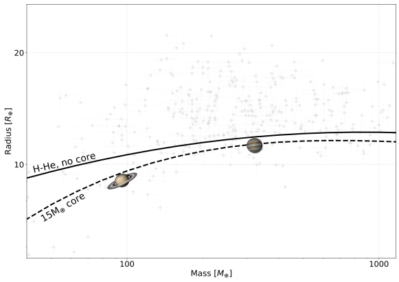
Figure 1: The mass-radius (M-R) relation of H-He-dominated planets. The solid black curve corresponds to a H-He composition with a proto-soar ratio. The dotted line demonstrates the influence of a $15M_{\oplus}{}$ heavy-element core on the M-R relation. Also shown are Jupiter and Saturn, and detected exoplanets in gray (from the Dace catalog (https://dace.unige.ch/dashboard/)).

In addition, since Saturn is farther from the pure-H-He curve than is Jupiter, it is expected to be more enriched with heavy elements. This prediction might appear to be contradicted by Saturn’s lower average density ($687\;\mathrm{kg~{}m^{-3}}$ compared with Jupiter’s $1326\;\mathrm{kg~{}m^{-3}}$). It’s the greater degree of compression of hydrogen and helium in Jupiter’s interior, due to its larger mass, that accounts for its higher overall bulk density.

2.2 Polytropic models

A step beyond the mass-radius relation is the unit-index polytrope, the relationship:

$$P=K\rho^{2}$$ (1)

between pressure $P$ and density $\rho$. This simple and artificial assumption can nevertheless be a surprisingly reasonable approximation of the compressibility of a hydrogen-helium mixture at conditions typical of giant planet envelopes, with the polytropic constant $K=2.1\times{10}^{12}\;\mathrm{m^{5}\,kg^{-1}\,s^{-2}}$.

The polytropic relation and the condition of hydrostatic equilibrium ($dP/dr=-\rho(r)g(r)$, where $g(r)$ is the local acceleration due to gravity) combine to an integro-differential equation on $\rho(r)$ which, with the assumption of a spherical planet (i.e., neglecting oblateness due to rotation), becomes the solvable ordinary differential equation

$$\frac{d}{dr}(r\frac{d\rho}{dr})=-k^{2}r^{2}\rho(r),$$ (2)

where $k=\frac{2\pi{G}}{K}$. Considering boundary conditions, the solution is

$$\rho(r)=\rho_{\text{c}}\frac{\sin(kr)}{kr}$$ (3)

for $0\leq{r}\leq{R=\sqrt{\frac{\pi{K}}{2G}}}$.

The prediction then is that, neglecting the effects of rotation, a core, and heavy elements, an isolated body in the giant planet mass regime should have a predictable radius, which comes out to $R=70,300\;\mathrm{km}$. Apparently the index-1 polytrope approximation is more appropriate for Jupiter than it is for Saturn. This is both because the $P\propto\rho^{2}$ approximation doesn’t fit Saturn’s present day envelope as well as Jupiter’s, and also that Saturn’s interior is more enriched with heavy elements compared with Jupiter, as we already suspected form the mass-radius relation.

More information on polytropic models, extended to account for rotation and sometimes a core, can be found in (Hubbard, 1975; Kramm et al., 2011; Paul et al., 2014).

3 Interior models

While the mass-radius and polytropic relations can be used to infer some basic predictions about the planetary bulk composition they provide no information on the distribution of the materials. In order to constrain the density profile, and therefore the material distribution, additional constraints are required. For solar-system gas giants a critical measurement is their gravitational fields. Additionally, the magnetic fields, 1-bar temperatures, atmospheric composition, and static and dynamic rotation states are available and provide further constraints. The key measurable properties of Jupiter and Saturn that are used in interior models are listed in Table 1.

Since giant planets consist of mostly fluid H and He, they do not have solid surfaces below the cloud layers and as a result the “surface” of the planet is defined as the location where the pressure is 1 bar, the pressure at the Earth’s surface. Often the measurement of the temperature at 1 bar is used to infer the entropy of the outer envelope and therefore of the planetary interior for adiabatic models where the temperature profile is set to be the adiabatic gradient (see Militzer et al. (2016) and references therein for details).

Property	Jupiter	Saturn
Distance to Sun (AU)	5.204	9.582
Mass ($10^{24}\;\mathrm{kg}$)	$1898.13\pm{}0.19$	$568.319\pm{}0.057$
Equatorial Radius (km)	71492$\pm$4	60268$\pm$4
Mean Density ($\mathrm{g/cm^{3}}$)	$1.3262\pm{}0.0004$	$0.6871\pm{}0.0002$
Effective Temperature (K)	$124.4\pm{}0.3$	$95.0\pm{}0.4$
1-bar Temperature (K)	$165\pm{}4$	$135\pm{}5$
Rotation Period${}^{\text{i}}$	9h 55m 29.56s	10h 39m $\pm\sim$10m
$J_{2}\times 10^{6}$	$14696.572\pm{}0.014$	$16290.557\pm{}0.028$
$J_{4}\times 10^{6}$	$-586.609\pm{}0.004$	$-935.318\pm{}0.044$
$J_{6}\times 10^{6}$	$34.24\pm{}0.24$	$86.334\pm{}0.112$
Love number $k_{2}$	$0.565\pm{}0.018$	$0.382\pm{}0.017$

Table 1: Basic observed properties of Jupiter and Saturn from Helled & Guillot (2018) and references therein. Gravity field data from Iess et al. (2018, 2019). The gravitational coefficients correspond to the reference equatorial radii of 71,492 km and 60,330 km for Jupiter and Saturn, respectively. ${}^{\text{i}}$see Helled et al. (2015); Fortney (2018) for discussion on Saturn’s rotation rate uncertainty.

An interior model of a giant planet is a self-consistent solution of the structure equations:

$$\frac{dm}{dr} =4\pi{}r^{2}\rho,$$ (4a)

$$\frac{1}{\rho}\frac{dP}{dr} =-\frac{Gm}{r^{2}}+\frac{2}{3}\omega^{2}r,$$ (4b)

$$\frac{dT}{dr} =\frac{T}{P}\frac{dP}{dr}\nabla{T},$$ (4c)

where $P$ is the pressure, $\rho$ is the density, $m$ is the mass inside a pressure level of mean radius $r$, and $\omega$ is the rotation rate. The first equation defines the transformation between a mass variable and radius variable. The second equation is the condition of hydrostatic equilibrium, including a correction term to account for oblateness due to uniform rotation. The third equation describes the energy transport outward from the interior of the object to its surface. The temperature gradient, $\nabla{T}\equiv{}d\ln{T}/d\ln{P}$ depends on the energy transport mechanism. In convective regions the temperature gradient is set to the adiabatic gradient $\nabla_{\text{ad}}=\frac{\partial\ln{T}}{\partial\ln{P}}\arrowvert_{S}$, where $S$ is the entropy. If the energy transport is by radiation, the diffusion approximation is

$$\nabla=\nabla_{\text{rad}}=\frac{3}{16\pi{}Gac}\frac{\kappa_{R}L_{r}P}{mT^{4}}=\left(\frac{\partial\ln{T}}{\partial\ln{P}}\right)_{\text{rad}}.$$ (5)

The derivative refers to the actual temperature–pressure variation in the planetary structure of the planet, and $\kappa_{\text{R}}$ is the Rosseland mean opacity. Often, radiation and conduction are treated together using an effective opacity that accounts also for the contribution of conduction. Finally, a fourth equation, the equation of state (EoS), relates the density, pressure, and temperature at each level. More details on the EoS are given in section 3.1.

The hydrostatic condition as expressed in eq. (4b) is only a first order approximation of the effects of rotation. The precise statement of the condition of hydrostatic equilibrium is this:

$$\frac{1}{\rho}\nabla{P}=-\nabla{U}$$ (6)

where $U=V+Q$ is the sum of gravitational potential $V(\mathbf{r})$ and centrifugal potential $Q(\mathbf{r})=-(1/2)\omega^{2}r^{2}\sin^{2}\theta$.

The gravitational potential field $V$ is

$$V(\vec{r})=-G\int d^{3}r^{\prime}\>\frac{\rho(\vec{r^{\prime}})}{|\vec{r^{\prime}}-\vec{r}|},$$ (7)

where the integration is over the, as yet unknown, volume of the planet. An expansion in powers of $r$ reads

$$V(r,\,\phi,\,\theta) = -\frac{GM}{r}\left[\sum_{n=0}^{\infty}\left(\frac{r}{a_{0}}\right)^{\!\!-n}\!\!\!J_{n}\>P_{n}(\mu)\right.$$

$$+ \left.\sum_{n=1}^{\infty}\sum_{m=1}^{n}\left(\frac{r}{a_{0}}\right)^{\!\!-n}\!\!\left(C_{nm}\>\cos m\phi\>+\>S_{nm}\>\sin m\phi\right)\>P_{n}^{m}(\mu)\right]$$ (8)

where $a_{0}$ denote the equatorial radius and $\mu=\cos{\theta}$. In this form the information about the planet’s mass distribution is contained in the coefficients $J_{n}$, $C_{nm}$, and $S_{nm}$. The zonal harmonics $J_{n}$ are

$$Ma_{0}^{n}J_{n}=-\int_{r^{\prime}<R}d^{3}r^{\prime}\rho{}r^{\prime n}P_{n}(\mu),$$ (9)

with $P_{n}$ the Legendre polynomials. The tesseral harmonics are

$$Ma_{0}^{n}C_{nm}=2\frac{(n-m)!}{(n+m)!}\int_{r^{\prime}<R}d^{3}r^{\prime}\rho(r^{\prime})(r^{\prime})^{n}\cos{m\phi^{\prime}}P_{n}^{m}(\mu^{\prime}),$$ (10)

and

$$Ma_{0}^{n}S_{nm}=2\frac{(n-m)!}{(n+m)!}\int_{r^{\prime}<R}d^{3}r^{\prime}\rho(r^{\prime})(r^{\prime})^{n}\sin{m\phi^{\prime}}P_{n}^{m}(\mu^{\prime}),$$ (11)

with $P_{n}^{m}$ the associated Legendre functions. Often, the longitudinal orientation of the planet-centered coordinate frame can be chosen so that $S_{nm}=0$. If the gravity field does not dependent on longitude at all, i.e., if the field is symmetric with respect to the rotation axis, also $C_{nm}=0$. If furthermore north-south symmetry with respect to the equatorial plane holds, the odd $J_{n}$ vanish as well. Finally, for spherical planet, all $J_{n>0}=0$.

Due to rotation, giant planets are oblate, raising the even $J_{2n}$. Winds perturb the density and thus introduce perturbation in the $J_{n}$. At first glance, the zonal bands on Jupiter and Saturn appear north/south symmetric, but a closer look at Jupiter shows this is not exactly the case. As a result, the odd $J_{n}$ are raised on Jupiter (Kaspi et al., 2018), and also Saturn (Iess et al., 2019). One may thus write:

$$J_{n}^{\mathrm{obs}}=J_{n}^{\mathrm{static}}+J_{n}^{\mathrm{dyn}}.$$ (12)

The static gravitational harmonics $J_{2n}$ depend on the internal density distribution, with the lower order harmonics $J_{2},J_{4}$ being sensitive down to $\sim 0.6\>R_{\rm J}$, while the static higher order harmonics probe the density distribution in the deep atmosphere. This behavior is illustrated in Fig. 2 that shows an example of a Jupiter structure model that fits the observed $J_{2}$ and $J_{4}$ values.

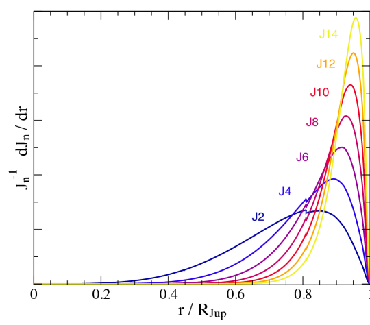
Figure 2: $J_{2n}$ contributions functions for a Jupiter model with Gaussian-Z in the deep interior below 0.5 $R_{\rm J}$, where only $J_{2}$ is still sensitive. At the small discontinuity seen in $J_{2}$ and $J_{4}$, an abrupt transition between He-poor and He-rich regions occurs.

For both Jupiter and Saturn precise measurements of their $J_{n}$ values are available from $J_{2}$ to $J_{12}$ (Durante et al., 2020; Iess et al., 2019). This allows to constrain their internal structures far beyond what can be obtained by mass and radius alone, as is the case for giant exoplanets. On Jupiter and Saturn, the high-order $J_{n}$ are primarily influenced by the winds, while the low-order moments $J_{2}$, $J_{4}$ primarily by the static field. The latter are thus used to constrain interior models. Different interior models differ in their prediction for $J_{6}$ and $J_{8}$ (Guillot et al., 2018; Nettelmann et al., 2021) and therefore place somewhat different constraints on the winds. Efforts to find an optimum model, which would yield optimum agreement with the low-order field and the observed wind speeds are still ongoing.

Eqs. (4) cannot be inverted to yield a unique solution. Instead, they are treated in a forward modeling framework. A model is proposed, by which we mean, some configuration of the planet’s composition. Starting with a guess for $P(r)$, the temperature profile is calculated with eq. (4c). The EoS is invoked to yield $\rho(r)$, then a procedure for calculating the potential, $V$. Finally the hydrostatic equilibrium equation is integrated to update $P(r)$. The process iteratively approaches a self-consistent solution, which is then checked against the known observables.

However, the solution is non-unique. The goal of such models could be a single, best-fitting model, most consistent with every observed quantity, or an exploration of all plausible models. Both approaches have been, and still are actively pursued, as we discuss in the sections on Jupiter (sec. 4) and Saturn (sec. 5).

3.1 The EoS of Hydrogen, Helium and Heavies

As discussed above, in order to model the structure of giant planets one needs to use an EoS in order to connect the density-pressure-temperature and other thermodynamic properties.

Giant planet interiors serve as natural laboratories for studying different elements at extreme conditions. In addition, calculating the EoS of materials in Jupiter and Saturn interior conditions is a challenging task because molecules, atoms, ions and electrons coexist and interact, and the pressure and temperature range varies by several orders of magnitude, going up to several tens of mega-bars (Mbar), or $\gtrsim{100}\;\mathrm{Gpa}$ and several $10^{4}$ Kelvins. Therefore, information on the EoS at such conditions requires performing high-pressure experiments and/or solving the many-body quantum mechanical problem to produce theoretical EoS tables that cover such a large range of pressures and temperatures. Despite the challenges, there have been significant advances in high-pressure experiments and ab initio EoS calculations. More information on that topic can be found in Fortney & Nettelmann (2010); Baraffe et al. (2014); Militzer et al. (2016); Guillot & Gautier (2015); Helled & Guillot (2018); Helled & Fortney (2020) and references therein.

The composition of both Jupiter and Saturn is dominated by hydrogen and helium (H, He), and therefore their modeling strongly depends on our understanding of these materials at planetary conditions.

Hydrogen

Our understanding of hydrogen at high pressures and temperatures is still incomplete and is a topic of intensive theoretical and experimental research (see Helled & Fortney (2020) and references therein). When it comes to giant planet models, it has to be acknowledged that the EoS to be used must cover a large range of temperatures (100 – 10⁵ K) and pressures (1 bar – 10s Mbar, since experiments are often limited to a specific range of parameters, planetary scientists must rely on EoS calculations that are calibrated by experiments.

One of the most widely used EoS for H-He for giant planets and brown dwarfs is the SCVH EoS (Saumon et al., 1995). This EoS based on an Helmholtz free-energy model, from which thermodynamic parameters like pressure and entropy are derived self-consistently. The SCvH EoS shows a first-order phase transition across a wide range in temperature ($\sim 10^{3}$–$2\times 10^{4}$K) and pressure ($\sim 0.1$–100 Mbar), which was interpreted as a possible plasma phase transition between molecular hydrogen and atomic, metallic hydrogen. This broad phase transition region is smoothed by interpolation. Unfortunately, this region corresponds to a region in the planetary deep interior that strongly affects the inferred gravitational moments ($J_{2}$, $J_{4}$, see Fig. 2).

An alternative approach that is more challenging computationally, is to simulate many-particle systems of electrons and ions, which basically obey the Coulomb force, to infer the EoS and other material properties. However, just 1g of hydrogen contains $5.98\times 10^{23}$ atoms, so approximations are still required. Out of the several variants of approximationsHelled & Fortney (2020), the method of DFT-MD simulations has been used to predict the EoS of H, He. In this method, the ions are treated by classical Monte Carlo simulations (MD), and the electrons by density functional theory (DFT). The electron wave functions and eigenvalues are calculated using so-called pseudo-potentials, which approach the Coulomb potential at sufficiently large interparticle distances to avoid strong oscillations at small distances. This method is particularly suited for high densities where Free-energy-based EoS show their largest uncertainties.

At present, there are three DFT-MD data based H EoS that are commonly used in the planetary community: MH13 EoS (Militzer & Hubbard, 2013), REoS Becker et al. (2014), and CMS19-EoS Chabrier et al. (2019). The MH13 EoS uses DFT-MD calculations and is calculated for a protosolar H-He mixture. It also provides the entropy. At lower densities, this EoS is connected to the SCvH EoS ensuring a smooth transition in entropy (and pressure). The R-EoS for H includes DFT-MD data between 0.1 and 10 g/cc.

Entropy values or adiabats are calculated using standard thermodynamic relations Scheibe et al. (2019). In the CMS19-EoS, DFT-MD data includes a small range of 0.3–5 g/cc and at lower densities, the SCvH EoS is employed. As a result of the DFT-MD data in these three EoSs, the molecular-metallic transition occurs at lower temperatures of a few 1000 K (see Fig. 3). For a comparison with experimental data and detailed discussions on EoSs we refer the reader to the cited literature. It was recently found that interior models of Jupiter and Saturn based on the DFT-MD H-He EoS data have a rather compressible adibat, meaning higher densities than for SCvH EOS at pressures where $J_{4}$ is sensitive. As a result, DFT-MD based models yield low metallcities in the outer envelopes of Jupiter and Saturn.

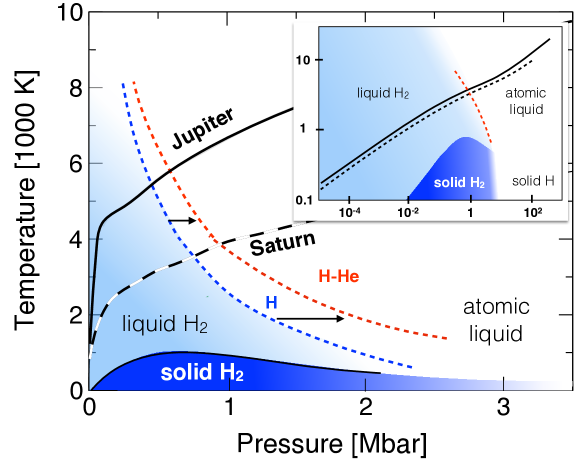
Figure 3: The phase diagram of hydrogen. Large panel: A zoom to the temperature-pressure region associated with hydrogen metallization. The blue and red dashed curves present the theoretical prediction of the fluid metallization of pure H and of a H-he mixture as inferred from QMC simulations Mazzola et al. (2018). Also shown are examples of pressure-temperature profiles for Jupiter (solid black curve) and Saturn (dashed curve). Small right panel: The H phase diagram on a larger pressure-temperature scale, showing the different phases of H, and representative solutions for Jupiter and Saturn. The image is modified from Mazzola et al. (2018); Helled & Fortney (2020).

Hydrogen-Helium

The second most common element in giant planets is Helium. Experimental data and numerical calculations of the phase diagram of H- He mixtures are now being performed. For giant planet interiors, a key feature of such a mixture is the immiscibility of He in H which is expected to lead to He settling, or “helium rain” Stevenson & Salpeter (1977b, a); Morales et al. (2013); Brygoo et al. (2021). The process of helium rain affects the cooling as well as the structure of giant planets Püstow et al. (2016); Mankovich & Fortney (2019). The conditions for de-mixing are still debated but it seems that Saturn’s interior, due to its lower temperature, is more affected by this process in comparison to Jupiter Schöttler & Redmer (2019). Understanding the behavior of a H-He mixture is also important since the existence of helium in H stabilizes the H molecules, and was found to delay the H metallization towards higher densities Mazzola et al. (2018).

Heavy elements

In astrophysics, heavy elements also known as “heavies” correspond to all elements that are heavier than hydrogen and helium. The heavy-element mass fraction is often represented by the letter “Z”. Heavy elements in giant planets can be metals (e.g., iron), silicates (e.g., silicon) or volatiles (e.g., oxygen, ammonia). Although understanding the internal structure of Jupiter and Saturn strongly depends on the H, and H-He EoS, a determination of the total mass of heavy elements and how they are distributed within the planetary interior is critical for our understanding of the formation and evolution of the giant planets (see Helled & Guillot (2018) and references therein for details).

Empirical EoS

An alternative approach to the EoS-based models described above is to parameterize the $\rho(r)$ configuration rather than the H-He-Z mixture configuration. The hydrostatic equation (4b), the temperature equation (4c), and the equation of state are dropped from the iterative solution cycle (although they can still be integrated after the fact) and the solution is required only to match the known mass, radius, and gravity field (and boundary conditions). This framework (which have long been termed “empirical”) seems like a step backwards from EoS-based models but the goal is different. While EoS-based solutions create very detailed, realistic, and easy to interpret model planets, they invariably rely on a host of assumptions, some made with sound physical reasoning and some made out of necessity, and thus are limited in the types of solutions that can be produced. Of course, composition-agnostic models are subject to their own assumptions and simplifications, required to parameterize the density profiles, but they are not subject to the same assumptions as EoS-based models, and in particular they are not required to assume homogeneous composition layers anywhere in the planet.

In this way, composition-agnostic models can be used to explore a wider range of plausible interiors. Examples of this approach applied to Saturn Movshovitz et al. (2020) and Jupiter Neuenschwander et al. (2021) are discussed in the respective sections. This approach also has been, and is being, applied to the Uranus and Neptune Marley et al. (1995); Podolak et al. (2000); Helled & Bodenheimer (2011).

4 Jupiter

Our understanding of Jupiter’s interior has been challenged when Jupiter’s gravitational field was accurately measured by the Juno spacecraft Iess et al. (2018). Jupiter structure models pre-Juno era can be found in Miguel et al. (2016); Militzer et al. (2016).

The much more accurate gravity data has led to the development of more complex structure models that include composition gradients and account for the dynamical contributions. Interestingly, the improvements in the quality of the gravity data led to many new questions regarding the planetary interiors, and standard structure models have been challenged.

Updated structure models that fit Juno data imply that Jupiter’s interior is characterized by a non homogeneous distribution of the heavy elements, where the deeper interior is more metal-rich Wahl et al. (2017b); Debras & Chabrier (2019). In addition, in these updated models Jupiter’s core is no longer viewed as a pure heavy-element central region with a density discontinuity at the core-envelope-boundary, but as a central region enriched with heavies but also consists of lighter elements such as H-He.Such a fuzzy/diluted core could extend to a few tens of percents of Jupiter’s total radius. The new Jupiter structure models also imply that the temperature profile in the planetary deep interior can significantly differ from the adiabatic one Vazan et al. (2018); Debras & Chabrier (2019). Overall, the total heavy-element mass in Jupiter can range between $\sim$ 20–60 M_⊕ (Helled, 2019).

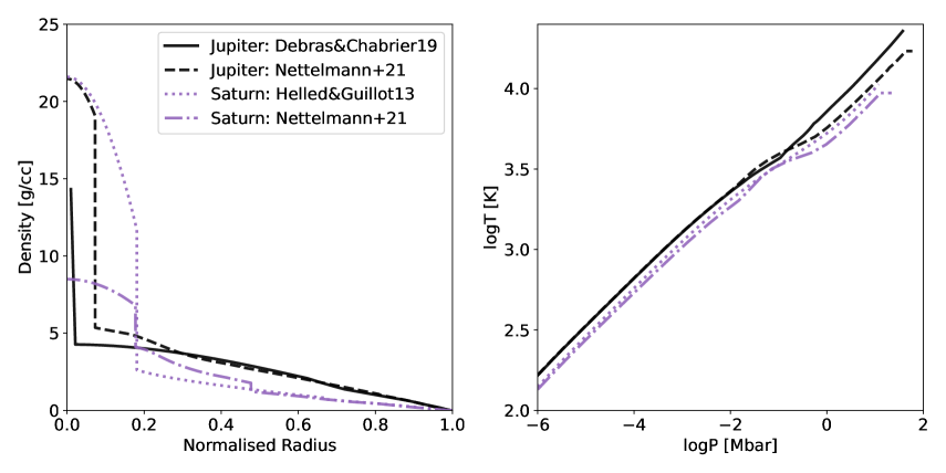
Figure 4: Examples of Jupiter (black) and Saturn (purple) structure models. Left: Density as a function of normalized radius. The different curves correspond to various models as indicated in the top-right panel of the figure. Right: Log-temperature vs. log-pressure of the models.

Interestingly, it was recently shown that the high-order $J_{n}$ of the Jupiter models fall along the same line in $J_{n}$–$J_{n+2}$ space, regardless of detailed model assumptions and the H-He EOS used (Guillot et al., 2018; Nettelmann et al., 2021). Nettelmann et al. Nettelmann et al. (2021) found that $J_{6}$ stands out in that it is neither adjusted, as $J_{2}$ and $J_{4}$ are, nor insensitive to interior model assumptions, as the higher order $J_{n}$ $n\geq 8$ are. As the wind contribution on Jupiter is small, $J_{6}$ further constrain the interior. For instance, it can be used to put limits on the transition pressure between the outer, He-poor outer envelope and the inner, He-rich envelope, where a best match was found for transition pressures of 2–2.5 Mbars (Nettelmann et al., 2021), which lies within the 0.9 Mbar–6 Mbar demixing region in Jupiter as inferred from reflectivity measurements (Brygoo et al., 2021). It was also shown that heavy-element gradients in the deep interior below $\sim$ 20 Mbar can lead to high metallicities of up to $Z=0.5$ at the compact core-mantle boundary, yielding a largely homogeneous-in-Z envelope atop. However, the atmospheric heavy-element abundance in recent adiabatic models with CMS-19 EoS was found to be substantially less than 1x solar, the $1\sigma$ lower limit of the equatorial water abundance observed by Juno (Li et al., 2020), suggesting that an adiabatic profile overestimates the density especially in the molecular envelope where $J_{4}$ is sensitive, see Figure 2. Representative density profiles and pressure-temperatures of Jupiter are shown in Fig. 4 in black. The solid and dashed curves correspond to Jupiter models as inferred by (Debras & Chabrier, 2019) and (Nettelmann et al., 2021).

5 Saturn

Modeling Saturn’s interior is also challenging. Saturn is brighter than predicted by fully convective models, suggesting that the effect of He rain and/or non-convective regions is more profound in Saturn. In addition, Saturn’s rotation rate is not as well determined. Several lines of evidence sees to be converging on an answer of about of 10 hours 33 minutes (see review by Fortney (2018) for details).Below, we summarize a few interior models of Saturn that fit Cassini gravity data. A detail review on Saturn can be found in (Fortney et al., 2018) and references therein.

Helled & Guillot (Helled & Guillot, 2013) presented 3-layer models of Saturn with a large range of model parameters using the SCVH EoS. For the range of different model assumptions, the inferred core mass and heavy-element mass in the envelope were found to range between $\sim$5 – 20 M_⊕ and 0–7 M_⊕, respectively.

Leconte & Chabrier (Leconte & Chabrier, 2013) investigated the possibility of double-diffusive convection in Saturn and suggested that Saturn’s interior could be dominated by composition gradients (and be non-adiabatic). Saturn’s core mass was inferred to be between 10 and 21 M_⊕ while the heavy-element mass is the envelope was found to have the range 10 – 36 $M_{\oplus}$. This solution for Saturn does not only fit the gravity data, but can also explain Saturn’s low luminosity due to the less efficient cooling of the planet. Since in this scenario heat transport (cooling) is less efficient, the deep interior can be much hotter, and the planet can accommodate larger amounts of heavy elements.

Militzer et al. (Militzer et al., 2019) presented recent structure models of Saturn assuming distinct layers using Monte Carlo sampling, and considering different rotation periods and core sizes. It was found that Saturn’s core mass varies between 15 and 18 $M_{\oplus}$ and that the heavy-element mass in the envelope is small, less than $5\;\mathrm{M_{\oplus}}$. A similar result, when using a 4-layer model of Saturn was presented by Ni Ni (2020), where the total heavy-element mass in Saturn was found to be 12 – 18 $M_{\oplus}$. Here Saturn’s interior was assumed to consist of a compact core surrounded by a fuzzy core.

Recent Saturn models have been also been presented by Mankovich & Fuller Mankovich & Fuller (2021). Here the interior structure models were designed to fit not just the gravitational moments ($J_{2}$, $J_{4}$ and $J_{6}$) but also the the $m=-2$ oscillation mode deduced from ring seismology. These structure models imply that Saturn has a large region that is stable against convection extending to $\sim\!\!{60\%}$ of Saturn’s radius, the interior consists of composition gradients and that its central density is moderately low, $\sim\!\!{6}\;\mathrm{g/cm^{3}}$ implying that also Saturn’s core is “fuzzy/dilute”.

Nettelmann et al. (Nettelmann et al., 2021) explored Saturn’s interior and compared the results when using different H-He EoSs. It was found that Saturn models with the CMS EoS result in enriched envelope that extends to $<0.4\>R_{\rm Sat}$ and compact heavy-element cores. Saturn was found to have a fuzzy core when accounting for EoS perturbations: then the core extends to $\sim 0.4R_{\rm Sat}$, a result that is more consistent with the solution of Mankovich & Fuller (2021). As discussed in detail in (Nettelmann et al., 2021), such a structure model corresponds to a dilute core and helium rain, which together result in a large region in Saturn’s deep interior that is inhomogeneous in composition and is stable against convection.

Examples of Saturn’s density profiles and pressure-temperature profiles are shown in Fig. 4 in purple. The dotted and dashed-dotted curves correspond to Saturn models presented by (Helled & Guillot, 2013) (Nettelmann et al., 2021).

6 Composition-agnostic Models

  

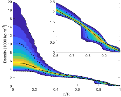
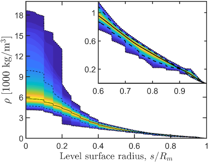
Figure 5: Left: Distribution of density profiles for Jupiter based on $8^{\text{th}}$-degree polynomials from (Neuenschwander et al., 2021). The black line marks the sample-median and the dashed lines the width of the one-sigma deviation. The color visualizes the sample distribution and comprises $\sim 96\%$ of all solutions. The polynomial-based profiles allow for up to two density jumps and have the same precision as the polytropic-based density structures. Right: The posterior probability distribution of Saturn’s density profiles inferred by (Movshovitz et al., 2020). The thick black line is the sample-median of density on each level surface. The dashed lines mark the the 16th and 84th percentiles and the dotted lines mark the 2nd and 98th percentiles; between the lines percentile value is indicated by color.

A different approach for interior modeling takes a more unbiased view on the planetary internal structure. This is by producing the so-called empirical structure models. In this case the planetary density profile is represented by a mathematical function, or via a series of random steps in density. Appropriate function for giant planet interiors include polynomials and polytropes. Then, by using the empirical representation for the density profile, all the profiles that match the observational constraint are inferred, and a solution for the pressure-density relation is found. From such models, the planetary composition can be indirectly inferred by searching for mixtures that can reproduce the density-pressure profile for an assumed temperature gradient using physical EoS.

The strength of empirical structure models is that they do not require knowledge of the behavior of elements at high pressures and temperatures, i.e., the EoS of the assumed materials. Also, they can probe solutions that are missed by the standard models, in particular, solutions that represent more complex interiors with various temperature profiles including sub- and super-adiabatic.

Recent empirical models of Jupiter were presented by Neuenschwander et al. (Neuenschwander et al., 2021). This study focused on the relation between the normalized moment of inertia and the gravitational moments using empirical density profiles represented by (up to) three polytropes. It was shown that models with a density discontinuity at $\sim$ 1 Mbar, as predicted by H-He phase separation simulations, correspond to a fuzzy core in Jupiter.

For Saturn, Movshovitz et al. (Movshovitz et al., 2020) applied a Bayesian MCMC-driven approach to explore the full range of possible density distributions in Saturn with density profiles parameterized as piecewise polynomial. These models exhibit densities in the outer parts of the planet suggesting significant heavy element enrichment (as expected), and while the inner half of Saturn was less well constrained most models exhibit significant density enhancement (interpreted as a core) but with density values consistent with dilute, rather than compact heavy-element core. Some density profiles as inferred by these studies are presented in Fig. 5.

7 Winds on Jupiter and Saturn

Jupiter’s visible atmosphere is structured into darker belts and brighter zones, which can be related to the winds that are blowing around the planet both in prograde and in retrograde direction with respect to the planet’s steady rotation. Strong zonal winds are also observed on Saturn. There are also upwellings and downdrafts through which heat from the deep interior is transported outward. Constraining the depth of the winds on Jupiter and Saturn was one of the main drivers for the Juno and the Cassini Grand Finale missions, respectively. For a recent review on thermal, compositional, and wind properties in the upper wind region we refer the reader to Kaspi et al. (2020); Guillot et al. (2022).

A depth of 1000 km corresponds to 1.3% of the radius of Jupiter, or 1.7% on Saturn. As can be estimated from Figure 2, density perturbations that reach as few percent in radius would reflect especially on the higher-order gravitational harmonics. Therefore, by measuring the high-order harmonics one obtains signatures on the depth of the winds. In addition, any signature in the measured odd gravity harmonics is a direct signature of the winds Kaspi (2013). Also it should be noted that while the low-order even harmonics are dominated by the deep interior, the wind also contribute to these harmonics, and are even more significant for $J_{6}$, $J_{8}$, and $J_{10}$ Kaspi et al. (2020).

The observed winds on Jupiter and Saturn can be mapped from the cloud level onto cylinders that rotate parallel to the planet’s spin axis Hubbard (1999); Kaspi et al. (2010); Kulowski et al. (2021). Such a vertical projection of the winds allowed Galanti et al. (2021) Galanti et al. (2021) to obtain a much better match to the high-order even $J_{n}$ than for a radial projection. This view is supported by 3D hydrodynamic simulations of zonal flows in rotating spherical shells (Dietrich et al., 2021).

By now there is general agreement that scale height of the wind decay depth is significantly less than the planet’s radius, but is much larger than the depth of water condensation. Regardless of the assumed decay depth profile. The exact wind braking mechanism is still not perfectly understood but is expected that the winds decay due to ohmic dissipation linked to the metallization of hydrogen Liu et al. (2008); Cao & Stevenson (2017).

While detailed models are still being developed, thanks to Juno and Cassini data the depth of the winds on the gas giants have been constrained Kaspi et al. (2020). The observed gravity and magnetic field data suggest that the depths of the flows on Jupiter and Saturn are $\sim 3000$ km and $\sim 9000$ km, respectively (Galanti & Kaspi, 2020; Kaspi et al., 2020). Nevertheless, further work is needed to better resolve the detailed wind structure and braking mechanism. It is also desirable to establish comprehensive giant planet models where the three aspects of flows, magnetic field, and internal structure are considered.

8 Love numbers

The tesseral harmonics $C_{nm}$ probe axial-asymmetric perturbations of the planetary gravity field. Such can arise from tides (Wahl et al., 2017a) or other effects. Due to their periodic nature, the tidal influence on the $C_{nm}$ can rather easily by extracted from the observed signal. The residuals will then be a probe of normal modes or other effects (see Iess et al (2018) Iess et al. (2018) for Jupiter and Iess et al (2019) Iess et al. (2019) for Saturn).

Planetary tidal response is commonly parameterized by the Love numbers $k_{nm}$, which are the linear response coefficients between the induced planetary gravitational field perturbation at the planet’s sub-satellite point $a_{s}$, and the gravity field of the perturber there, $W(a_{s})$. If the satellite orbits in the equatorial plane, $a_{s}=a_{0}$. Writing the planetary gravitational $V$ as:

$$V(r,\,\varphi,\,\theta)=V_{0}(r)+\sum_{n=2}^{\infty}V_{n}+\sum_{n=2}^{\infty}V_{n}+\sum_{n=1}\sum_{m=1}^{n}V_{nm},$$ (13)

where $V_{0}$ is the spherically symmetric part, and the gravity field $W$ of the tide-raisig perturber as

$$W=\sum_{n=0}^{\infty}W_{n}+\sum_{n=1}^{\infty}\sum_{m=1}^{n}W_{nm}$$ (14)

one can define the Love numbers of a fluid body as $k_{nm}=V_{nm}/W_{nm}$. If the planet resides in a (equilibrium) state of 1:1 spin-orbit resonance with its tidal perturber so that the tidal buldge raised by the satellite on the planet is static in the frame corotating with the planet, _knm can be obtained from expression (3) and written as:

$$k_{nm}^{static}=-\frac{3}{2}\>\frac{(n+m)!}{(n-m)!}\>\frac{C_{nm}}{q_{tid}\>P_{n}^{m}(\mu_{S})}\>\left(\frac{r_{S}}{R_{eq}}\right)^{n-2}\>.$$ (15)

and be computed from an interior model Wahl et al. (2017a).

In general, tides are a dynamic phenomenon. The tidal buldge floats around the planet, and to Coriolis force acts on that flow (Idini & Stevenson, 2021). Similar to the $J_{n}$–wind effect, one may write:

$$k_{nm}=k_{nm}^{static}+\Delta k_{nm}^{dyn}.$$ (16)

Cassini Lainey et al. (2017) and Juno measurements (Durante et al., 2020) revealed that the observed $k_{22}$ values are close to their static values, which for Jupiter is $k_{2}=0.5897$ Nettelmann (2019); Wahl et al. (2020) with an uncertainty of less than 0.02%, as the underlying interior models are already well constrained by the precisely measured $J_{2}$ and $J_{4}$ values. By analyzing 10 Juno passes, Durante et al. (2020) were able to reduce the $3\sigma$ uncertainty in $k_{22}$ to only 3%, revealing a clear deviation of 1–7% from the static value. Dynamic contributions to the Love numbers have thus observationally been found to exist on Jupiter (Idini & Stevenson, 2021), however, their quantitative computation is challenging can can arise from different physical origins.

Consequently, Idini and Stevenson Idini & Stevenson (2021) as well as Lai Lai (2021) aimed to explain the observed dynamic contributions. Idini and Stevenson Idini & Stevenson (2021) showed that including the tidal flow (but ignoring the Coriolis force) increases $k_{22}$ by $\sim$13% with respect to the static value of a non-rotating $n=1$ polytrope. Including Coriolis adds a negative dynamic correction bringing the observed value (0.565) into agreement with the superposition of $k_{2}^{static}+k_{2}^{dyn}$. Interestingly, the same procedure applied to $k_{42}$ yields a correction of an opposite sign to what has been observed Idini & Stevenson (2021); Lai (2021)).

To some extend, the $k_{nm}$ ’measurements’ rely on simplifications made in the fitting procedure of Juno’s trajectory. The reported values Durante et al. (2020) are based on satellite-independent $k_{nm}$ values, while it has been shown Wahl et al. (2017a); Nettelmann (2019); Wahl et al. (2020) that the static $k_{nm}$ differ as a function of the tidal forcing parameter $q_{\rm tid}=-3(M_{S}/M_{p})/(Req/a_{S})$, which differs among satellites of different masses $M_{S}$ and orbital distances $a_{S}$. The observational determination of Jupiter’s tidal response coefficients is still ongoing and is a key goal of Juno’s extended mission. Further moments showing signs of dynamic influence are $k_{42}$ and $k_{44}$ Idini & Stevenson (2021).

Love number observations provide a new opportunity to further constrain the internal structure of giant planets. As discussed above, both Jupiter and Saturn could posses thick stably stratified deep interiors and further stable regions in the envelope where g-modes can exist. If they fall in resonance with the tidal forcing frequency they can significantly influence the tidal response. Since broadening and shifts of the resonance depend on the location and width of the stably stratified region Lai (2021), the tidal response enhancement can even occur out-of-resonance Lai (2021). This effect enables us to investigate the width and location of possible stratified layers.

9 Summary & Outlook

Giant planets are key objects to characterize as their composition and internal structure reveal key information for formation theories and on the conditions of the protoplanetary disks where the planets formed.

Our understanding of giant planet interiors has been revolutionized in the last several years thanks to the accurate data from the Juno and Cassini missions. It is now clear that both planets have complex interiors that include non-convective regions, composition gradients and fuzzy cores. Figure 6 provides a schematic representation of the internal structures of Jupiter and Saturn. While great progress has been made, new questions have arisen and much work and future investigations are required.

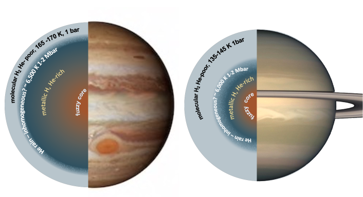
Figure 6: Sketches of the internal structures of Jupiter and Saturn. The outer layers of both planets is expected to mostly consist of molecular hydrogen. Due to the process of helium rain the outer envelope is depleted in helium, and there is a region where helium rain takes place. The inner part of the planets consists of metallic hydrogen with enriched helium, and possibly composition gradients and/or fuzzy core that can extend to more than half of the planetary radius (see text for further details). The exact heavy-element mass and its distribution is still being investigated. Figure modified from Helled (2019).

Such future investigations may include:

• A detailed comparative planetology should be obtained by having similar observables for Jupiter and Saturn, such as has been achieved for the gravity and wind velocity measurements. For example, at present, only for Jupiter are atmospheric elemental abundances measured below the radiative-convective boundary. Their vertical abundance profiles are particularly valuable as these elements do not condense. Therefore a probe to directly measure the atmospheric composition of Saturn is clearly desirable. Such a probe can determine the He abundance in Saturn’s atmosphere, constraining the magnitude of He rain, and determining Saturn’s atmospheric metallicity.

• Jovian seismology could further constrain the planetary structure. For example, the detection and characterization of planetary f/g-modes as been detected in Saturn’s rings, doppler imaging, and measurements of the dynamic parts of the Love numbers. In that regard, Juno extended mission is on its way to let us look deep into Jupiter’s interior of Jupiter via improved gravity measurements.

• The calculated structure depends on the used EoS as small differences in the EoS can lead to relatively large differences in the inferred composition. As a result, it is clear that further investigations (both theoretically and experimentally) of materials at planetary conditions are desirable.

• A detailed comparison between Jupiter and Saturn and giant exoplanets. Using the observed trends and inferred compositions and structure of a large number of giant exoplanets can be used to put Jupiter and Saturn in perspective, and at the same time the detailed investigation of the solar system giant planets is key to test and assess the nature of gas giant planets.

Overall, it seems that current models of Jupiter and Saturn have cannot reproduce all the observed measurements at once. Interior models of both Jupiter and Saturn typically predict relatively low envelope metallicities: solar or sub-solar, which is at odds with observations Atreya et al. (2016); Guillot et al. (2022). This could imply that the measured atmospheric metallicities do not represent the bulk composition of the outer envelope and/or that our models are based on inappropriate assumptions/steups such as the applied EoS, the entropy assigned, or the assumed temperature profile. We hope that future investigations will reconcile this issue sand will lead to a more comprehensive understanding of Jupiter and Saturn.

References

- Atreya et al. (2016) Atreya, S. K., Crida, A., Guillot, T., et al. 2016, ArXiv e-prints 1606.04510. https://arxiv.org/abs/1606.04510
- Baraffe et al. (2014) Baraffe, I., Chabrier, G., Fortney, J. J., & Sotin, C. 2014, in Protostars Planets VI, ed. H. Henning, T.K, Dullemond, C.P., Klessen, R.S., Beuther (Tucson, AZ: University of Arizona Press), 763–786
- Becker et al. (2014) Becker, A., Lorenzen, W., Fortney, J. J., et al. 2014, Astrophys. J. Suppl. Ser., 215, 21, doi: 10.1088/0067-0049/215/2/21
- Brygoo et al. (2021) Brygoo, S., Loubeyre, P., Millot, M., et al. 2021, Nature, 593, 517, doi: 10.1038/s41586-021-03516-0
- Cao & Stevenson (2017) Cao, H., & Stevenson, D. J. 2017, Icarus, 296, 59, doi: https://doi.org/10.1016/j.icarus.2017.05.015
- Chabrier et al. (2019) Chabrier, G., Mazevet, S., & Soubiran, F. 2019, Astrophys. J., 872, 51, doi: 10.3847/1538-4357/aaf99f
- Debras & Chabrier (2017) Debras, F., & Chabrier, G. 2017, A&A, 97, doi: 10.1051/0004-6361/201731682
- Debras & Chabrier (2019) —. 2019, Astrophys. J., 872, 100, doi: 10.3847/1538-4357/aaff65
- Dietrich et al. (2021) Dietrich, W., Wulff, P., Wicht, J., & Christensen, U. R. 2021, Mon. Not. R. Astron. Soc., 505, 3177, doi: 10.1093/mnras/stab1566
- Durante et al. (2020) Durante, D., Parisi, M., Serra, D., et al. 2020, Geophys. Res. Lett., 47, doi: https://doi.org/10.1029/2019GL086572
- Fortney (2018) Fortney, J. J. 2018, Nature, 555, 168, doi: 10.1038/d41586-018-02612-y
- Fortney et al. (2018) Fortney, J. J., Helled, R., Nettelmann, N., et al. 2018, in Saturn 21st Century, ed. K. H. Baines, M. F. Flasar, N. Krupp, & T. Stallard (Cambridge University Press), 44–68
- Fortney & Nettelmann (2010) Fortney, J. J., & Nettelmann, N. 2010, Space Sci. Rev., 152, 423, doi: 10.1007/s11214-009-9582-x
- Galanti & Kaspi (2020) Galanti, E., & Kaspi, Y. 2020, Mon. Not. R. Astron. Soc., 501, 2352, doi: 10.1093/mnras/staa3722
- Galanti et al. (2021) Galanti, E., Kaspi, Y., Duer, K., et al. 2021, Geophys. Res. Lett., 48, doi: https://doi.org/10.1029/2021GL092912
- Guillot et al. (2022) Guillot, T., Fletcher, L., Helled, R., et al. 2022, PPVII, 0, 0
- Guillot & Gautier (2015) Guillot, T., & Gautier, D. 2015, in Treatise Geophys. (Second Ed., ed. G. Schubert (Oxford: Elsevier), 529–557
- Guillot et al. (2018) Guillot, T., Miguel, Y., Militzer, B., et al. 2018, Nature, 555, 227, doi: 10.1038/nature25775
- Helled (2019) Helled, R. 2019, in Oxford Res. Encycl. Planet. Sci. (Oxford: Oxford University Press)
- Helled & Bodenheimer (2011) Helled, R., & Bodenheimer, P. 2011, Icarus, 211, 939, doi: 10.1016/j.icarus.2010.09.024
- Helled & Fortney (2020) Helled, R., & Fortney, J. J. 2020, arXiv e-prints, arXiv:2007.10783. https://arxiv.org/abs/2007.10783
- Helled et al. (2015) Helled, R., Galanti, E., & Kaspi, Y. 2015, Nature, doi: 10.1038/nature14278
- Helled & Guillot (2013) Helled, R., & Guillot, T. 2013, Astrophys. J., 767, doi: 10.1088/0004-637X/767/2/113
- Helled & Guillot (2018) —. 2018, Internal Structure of Giant and Icy Planets: Importance of Heavy Elements and Mixing, ed. H. J. Deeg & J. A. Belmonte (Cham: Springer International Publishing), 167–185
- Hubbard (1975) Hubbard, W. B. 1975, Sov. Astron., 51, 1052
- Hubbard (1999) —. 1999, Icarus, 137, 357, doi: https://doi.org/10.1006/icar.1998.6064
- Hubbard et al. (2014) Hubbard, W. B., Schubert, G., Kong, D., & Zhang, K. 2014, Icarus, 242, 138, doi: 10.1016/j.icarus.2014.08.014
- Idini & Stevenson (2021) Idini, B., & Stevenson, D. J. 2021, Planet. Sci. J., 2, 69, doi: 10.3847/PSJ/abe715
- Iess et al. (2018) Iess, L., Folkner, W. M., Durante, D., et al. 2018, Nature, 555, 220, doi: 10.1038/nature25776
- Iess et al. (2019) Iess, L., Militzer, B., Kaspi, Y., et al. 2019, Science (80-. )., 2965, eaat2965, doi: 10.1126/science.aat2965
- Kaspi (2013) Kaspi, Y. 2013, Geophys. Res. Lett., 40, 676, doi: https://doi.org/10.1029/2012GL053873
- Kaspi et al. (2020) Kaspi, Y., Galanti, E., Showman, A. P., et al. 2020, Space Sci. Rev., 216, 84, doi: 10.1007/s11214-020-00705-7
- Kaspi et al. (2010) Kaspi, Y., Hubbard, W. B., Showman, A. P., & Flierl, G. R. 2010, Geophys. Res. Lett., 37, doi: https://doi.org/10.1029/2009GL041385
- Kaspi et al. (2018) Kaspi, Y., Galanti, E., Hubbard, W. B., et al. 2018, Nature, 555, 223, doi: 10.1038/nature25793
- Kong et al. (2013) Kong, D., Zhang, K., & Schubert, G. 2013, Astrophys. J., 764, 67, doi: 10.1088/0004-637X/764/1/67
- Kramm et al. (2011) Kramm, U., Nettelmann, N., Redmer, R., & Stevenson, D. J. 2011, A&A, 528, A18, doi: 10.1051/0004-6361/201015803
- Kulowski et al. (2021) Kulowski, L., Cao, H., Yadav, R. K., & Bloxham, J. 2021, J. Geophys. Res. Planets, doi: 10.1029/2020JE006795
- Lai (2021) Lai, D. 2021, Planet. Sci. J., 2, 122, doi: 10.3847/PSJ/ac013b
- Lainey et al. (2017) Lainey, V., Jacobson, R. A., Tajeddine, R., et al. 2017, Icarus, 281, 286, doi: https://doi.org/10.1016/j.icarus.2016.07.014
- Leconte & Chabrier (2013) Leconte, J., & Chabrier, G. 2013, Nat. Geosci., 6, 347, doi: 10.1038/ngeo1791
- Li et al. (2020) Li, C., Ingersoll, A., Bolton, S., et al. 2020, Nat. Astron., 4, 609, doi: 10.1038/s41550-020-1009-3
- Liu et al. (2008) Liu, J., Goldreich, P. M., & Stevenson, D. J. 2008, Icarus, 196, 653, doi: https://doi.org/10.1016/j.icarus.2007.11.036
- Mankovich & Fortney (2019) Mankovich, C., & Fortney, J. J. 2019, Astrophys. J., 889, 51
- Mankovich & Fuller (2021) Mankovich, C., & Fuller, J. 2021, Nat. Astron., doi: 10.1038/s41550-021-01448-3
- Marley et al. (1995) Marley, M. S., Gomez, P., & Podolak, M. 1995, J. Geophys. Res., 100, 23,349, doi: 10.1029/95JE02362
- Mazzola et al. (2018) Mazzola, G., Helled, R., & Sorella, S. 2018, Phys. Rev. Lett., 120, 25701, doi: 10.1103/PhysRevLett.120.025701
- Miguel et al. (2016) Miguel, Y., Guillot, T., & Fayon, L. 2016, Astron. Astrophys., 596, doi: 10.1051/0004-6361/201629732
- Militzer & Hubbard (2013) Militzer, B., & Hubbard, W. B. 2013, Astrophys. J., 774, 148
- Militzer et al. (2016) Militzer, B., Soubiran, F., Wahl, S., & Hubbard, W. B. 2016, J. Geophys. Res. Planets, 121, 1552, doi: 10.1002/2016JE005080
- Militzer et al. (2019) Militzer, B., Wahl, S., & Hubbard, W. B. 2019, Astrophys. J., 879, 78
- Morales et al. (2013) Morales, M. A., Hamel, S., Caspersen, K., & Schwegler, E. 2013, Phys. Rev. B, 87, 174105, doi: 10.1103/PhysRevB.87.174105
- Movshovitz et al. (2020) Movshovitz, N., Fortney, J. J., Mankovich, C., Thorngren, D., & Helled, R. 2020, Astrophys. J., 891, 109, doi: 10.3847/1538-4357/ab71ff
- Nettelmann (2019) Nettelmann, N. 2019, Astrophys. J., 874, 156, doi: 10.3847/1538-4357/ab0c03
- Nettelmann et al. (2021) Nettelmann, N., Movshovitz, N., Ni, D., et al. 2021, arXiv e-prints. https://arxiv.org/abs/2110.15452
- Neuenschwander et al. (2021) Neuenschwander, B. A., Helled, R., Movshovitz, N., & Fortney, J. J. 2021, Astrophys. J., 910, 38, doi: 10.3847/1538-4357/abdfd4
- Ni (2020) Ni, D. 2020, Astron. Astrophys., 639, A10, doi: 10.1051/0004-6361/202038267
- Paul et al. (2014) Paul, G. C., Barman, M. C., & Mohit, A. A. 2014, NRIAG J. Astron. Geophys., 3, 163, doi: 10.1016/j.nrjag.2014.10.003
- Podolak et al. (2000) Podolak, M., Podolak, J., & Marley, M. 2000, Planet. Space Sci., 48, 143, doi: 10.1016/S0032-0633(99)00088-4
- Püstow et al. (2016) Püstow, R., Nettelmann, N., Lorenzen, W., & Redmer, R. 2016, Icarus, 267, 323, doi: https://doi.org/10.1016/j.icarus.2015.12.009
- Saumon et al. (1995) Saumon, D., Chabrier, G., & van Horn, H. M. 1995, Astrophys. J. Suppl. v.99, 99, 713, doi: 10.1086/192204
- Scheibe et al. (2019) Scheibe, L., Nettelmann, N., & Redmer, R. 2019, Astron. Astrophys., 632, A70, doi: 10.1051/0004-6361/201936378
- Schöttler & Redmer (2019) Schöttler, M., & Redmer, R. 2019, J. Plasma Phys., 85, doi: 10.1017/S0022377819000199
- Stevenson & Salpeter (1977a) Stevenson, D. J., & Salpeter, E. 1977a, Astrophys. J. Suppl. Ser., 35, 239, doi: 10.1086/190479
- Stevenson & Salpeter (1977b) Stevenson, D. J., & Salpeter, E. E. 1977b, Astrophys. J. Suppl. Ser., 35, 221
- Vazan et al. (2018) Vazan, A., Helled, R., & Guillot, T. 2018, Astron. Astrophys., 14, 1, doi: 10.1051/0004-6361/201732522
- Wahl et al. (2017a) Wahl, S., Hubbard, W. B., & Militzer, B. 2017a, Icarus, 282, 183, doi: https://doi.org/10.1016/j.icarus.2016.09.011
- Wahl et al. (2017b) Wahl, S., Hubbard, W. B., Militzer, B., et al. 2017b, Geophys. Res. Lett., 44, 4649, doi: 10.1002/2017GL073160
- Wahl et al. (2020) Wahl, S. M., Parisi, M., Folkner, W. M., Hubbard, W. B., & Militzer, B. 2020, Astrophys. J., 891, 42, doi: 10.3847/1538-4357/ab6cf9
- Wisdom & Hubbard (2016) Wisdom, J., & Hubbard, W. B. 2016, Icarus, 267, 315, doi: 10.1016/j.icarus.2015.12.030