Scaling of acceleration statistics in high Reynolds number turbulence

Abstract

The scaling of acceleration statistics in turbulence is examined by combining data from the literature with new data from well-resolved direct numerical simulations of isotropic turbulence, significantly extending the Reynolds number range. The acceleration variance at higher Reynolds numbers departs from previous predictions based on multifractal models, which characterize Lagrangian intermittency as an extension of Eulerian intermittency. The disagreement is even more prominent for higher-order moments of the acceleration. Instead, starting from a known exact relation, we relate the scaling of acceleration variance to that of Eulerian fourth-order velocity gradient and velocity increment statistics. This prediction is in excellent agreement with the variance data. Our work highlights the need for models that consider Lagrangian intermittency independent of the Eulerian counterpart.

Introduction:

The acceleration of a fluid element in a turbulent flow, given by the Lagrangian derivative of the velocity, resulting from the balance of forces acting on it, is arguably the simplest descriptor of its motion. This is directly reflected in the Navier-Stokes equations:

$${\mathbf{a}}=D{\mathbf{u}}/Dt=-\nabla p+\nu\nabla^{2}{\mathbf{u}}+\mathbf{f}\ ,$$ (1)

where, ${\mathbf{u}}$ is the divergence-free velocity ($\nabla\cdot{\mathbf{u}}=0$), $p$ the kinematic pressure, $\nu$ is the kinematic viscosity and $\mathbf{f}$ is a forcing-term. Besides its fundamental role in the study of turbulence La Porta et al. (2001); Toschi and Bodenschatz (2009); Stelzenmuller et al. (2017); Buaria et al. (2020a), understanding the statistics of acceleration is of paramount importance for diverse range of applications constructed around stochastic modeling of transport phenomena in turbulence Sawford (1991); Wyngaard (1992); Pope (1994); Wilson and Sawford (1996). The application of Kolmogorov’s 1941 phenomenology implies that the variance (and higher-order moments) of any acceleration component $a$ can be solely described by the mean-dissipation rate $\langle\epsilon\rangle$ and $\nu$ Kolmogorov (1941); Heisenberg (1948); Yaglom (1949):

$$\langle a^{2}\rangle=\frac{1}{3}\langle|\mathbf{a}|^{2}\rangle=a_{0}\ \langle\epsilon\rangle^{3/2}\nu^{-1/2}\ ,$$ (2)

where $a_{0}$ is thought to be a universal constant.

However, extensive numerical and experimental work has shown that $a_{0}$ increases with Reynolds number Yeung and Pope (1989); Vedula and Yeung (1999); Gotoh and Rogallo (1999); Voth et al. (2002); Sawford et al. (2003); Mordant et al. (2004); Gylfason et al. (2004); Yeung et al. (2006); Ishihara et al. (2007). Thus, obtaining data on $a_{0}$ and modeling its $R_{\lambda}$-variation has been a topic of considerable interest. While several theoretical works have focused on acceleration statistics Hill (2002); Reynolds (2003); Beck (2007); Bentkamp et al. (2019), the most notable procedure – but whose validity should not be taken for granted – stems from the multifractal model Borgas (1993); Chevillard et al. (2003); Biferale et al. (2004), which quantifies acceleration intermittency (and, in general, the intermittency of other Lagrangian quantities) by adapting to the Lagrangian viewpoint the well-known Eulerian framework, based either on the energy dissipation rate Sreenivasan and Antonia (1997) or velocity increments Frisch (1995). A key result from this consideration is that $a_{0}\sim R_{\lambda}^{\chi}$, $\chi\approx 0.135$, where $R_{\lambda}$ is the Taylor-scale Reynolds number. While data from direct numerical simulations (DNS) and experiments do not directly display this power-law, it was nevertheless presumed to to be asymptotically correct at very large $R_{\lambda}$, and an empirical interpolation formula Sawford et al. (2003); Yeung et al. (2006),

$$a_{0}\simeq\frac{c_{1}R_{\lambda}^{\chi}}{(1+c_{2}/R_{\lambda}^{1+\chi})}\ ,$$ (3)

with $\chi=0.135$, $c_{1}=1.9$, $c_{2}=85$, was suggested to fit the data, showing reasonable success Sawford et al. (2003). An alternative scaling: $a_{0}\sim R_{\lambda}^{0.25}$ was proposed by Hill Hill (2002), which was indistinguishable from Eq.(3) at low-$R_{\lambda}$ Sawford et al. (2003); Ishihara et al. (2007); we discuss the veracity of this proposal later.

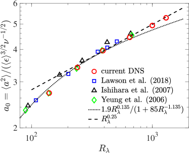
Figure 1: Normalized acceleration variance $a_{0}=\langle a^{2}\rangle/(\langle\epsilon\rangle^{3/2}\nu^{-1/2})$ as a function of $R_{\lambda}$. The data can be prescribed by a simple $R_{\lambda}^{0.25}$ power-law at high $R_{\lambda}$, in contrast to the previously proposed empirical fit given by Eq. (3).

In this Letter, we revisit the scaling of acceleration variance (and higher-order moments) by presenting new DNS data at higher $R_{\lambda}$. The new variance data agrees with previous lower $R_{\lambda}$ data, where the $R_{\lambda}$ range overlaps, but increasing deviations from Eq. (3) occur at higher $R_{\lambda}$. Results for high-order moments show even stronger deviations from previous predictions. Further analysis shows that the extension of Eulerian multifractal models to the Lagrangian viewpoint is the source of this discrepancy. We develop a statistical model which shows excellent agreement with variance data at high $R_{\lambda}$, and also provide an updated interpolation fit to include low $R_{\lambda}$ data.

Direct Numerical Simulations:

The DNS data utilized here correspond to the canonical setup of forced stationary isotropic turbulence in a periodic domain Ishihara et al. (2009), allowing the use of highly accurate Fourier pseudo-spectral methods Rogallo (1981). The novelty is that we have simultaneously achieved very high Reynolds number and the necessary grid resolution to accurately resolve the small-scales Buaria et al. (2019); Buaria and Sreenivasan (2020). The data correspond to the same Taylor-scale Reynolds number $R_{\lambda}$ range of $140-1300$ attained in recent studies Buaria et al. (2020b, c); Buaria and Pumir (2021); Buaria et al. (2022), which have adequately established convergence with respect to resolution and statistical sampling. The grid resolution is as high as $k_{\rm max}\eta_{K}\approx 6$ which is substantially higher than $k_{\rm max}\eta_{K}\approx 1-2$, utilized in previous acceleration studies Sawford et al. (2003); Yeung et al. (2006); Ishihara et al. (2007); $k_{\rm max}=\sqrt{2}N/3$ is the maximum resolved wavenumber on a $N^{3}$ grid and $\eta_{K}=\nu^{3/4}\langle\epsilon\rangle^{-1/4}$ is the Kolmogorov length scale. This improved small-scale resolution is especially necessary for capturing higher-order statistics of acceleration, since acceleration is even more intermittent than spatial velocity gradients Yeung and Pope (1989); Yeung et al. (2006).

Acceleration variance:

Figure 1 shows the compilation of data from various sources including data from both DNS Yeung et al. (2006); Ishihara et al. (2007) and bias-corrected experiments Lawson et al. (2018). We have also included DNS data obtained directly from Lagrangian trajectories of fluid particles Buaria et al. (2015, 2016); Buaria and Yeung (2017), which give identical results for acceleration variance . As evident, while Eq. (3) works for the previous range of $R_{\lambda}$, it does not fit the new data. In fact, a $R_{\lambda}^{0.25}$ scaling is more appropriate at higher $R_{\lambda}$, and as discussed later, the failure of multifractal models in fitting higher-order moments is even more conspicuous. To gain clarity on this point, it is useful to discuss the multifractal models first.

Acceleration scaling from multifractals:

The key idea in multifractal approaches is to quantify the intermittency of acceleration in terms of the intermittency of Eulerian velocity gradients or dissipation rate. Assuming a simple phenomenological equivalence between temporal and spatial derivatives, acceleration can be written in terms of dissipation rate and viscosity as $a\sim\epsilon^{3/4}\nu^{-1/4}$. Thus, the moments of acceleration are obtained as:

$$\langle a^{p}\rangle\sim\langle\epsilon^{3p/4}\rangle\nu^{-p/4}\ .$$ (4)

Alternatively,

$$\langle a^{p}\rangle/\langle a_{\rm K}^{p}\rangle\sim\langle\epsilon^{3p/4}\rangle/\langle\epsilon\rangle^{3p/4}\ ,$$ (5)

where $a_{\rm K}=\langle\epsilon\rangle^{3/4}\nu^{-1/4}$, i.e., acceleration based on Kolmogorov variables. Since Eulerian intermittency dictates that $\langle\epsilon^{q}\rangle\neq\langle\epsilon\rangle^{q}$ for any $q\neq 1$ Frisch (1995); Sreenivasan and Antonia (1997), the key assumption in its extension to Lagrangian intermittency is that the $p$-th moment of acceleration scales as the $(3p/4)$-th moment of $\epsilon$ Borgas (1993); Biferale et al. (2004). The scaling of $\langle\epsilon^{q}\rangle/\langle\epsilon\rangle^{q}$ can be obtained by several approaches, all leading to similar results. We briefly summarize a few approaches below, with additional details in the Supplementary Material sup .

The most direct approach is to utilize the multifractality of dissipation-rate Meneveau and Sreenivasan (1991); Borgas (1993). Within the multifractal framework, a scale-averaged dissipation $\epsilon_{r}$, over scale $r$, is assumed to be Hölder continuous: $\epsilon_{r}/\langle\epsilon\rangle\sim(r/L)^{\alpha-1}$, where $\alpha$ is the local Hölder exponent, with a corresponding multifractal spectrum $F(\alpha)$ and $L$ is the large-scale length. Note, the 1D spectrum $f(\alpha)$ is more common in the literature Meneveau and Sreenivasan (1991), which is simply: $f(\alpha)=F(\alpha)-2$. Now, $\epsilon_{r}$ reduces to the true dissipation for a viscous-cutoff defined as: $r\simeq(\nu^{3}/\epsilon_{r})^{1/4}$ or equivalently, $r/L\simeq Re^{-3/(3+\alpha)}$. Here, $Re=u^{\prime}L/\nu$, $u^{\prime}$ being the large-scale velocity; we also use $Re\sim R_{\lambda}^{2}$ and $\langle\epsilon\rangle\sim u^{\prime 3}/L$ from dissipation anomaly Sreenivasan (1984).

The above framework leads to the result:

$$\langle\epsilon^{q}\rangle/\langle\epsilon\rangle^{q}\sim R_{\lambda}^{\tau_{q}}\ ,\ \ \tau_{q}=\sup_{\alpha}\frac{6[q(1-\alpha)-3+F(\alpha)]}{3+\alpha}\ .$$ (6)

An approximation for $F(\alpha)$, such as the $p$-model Meneveau and Sreenivasan (1987, 1991), can be used to obtain $\tau_{q}$. The $p$-th moment of acceleration can then be simply obtained as

$$\langle a^{p}\rangle/a_{\rm K}^{p}\sim R_{\lambda}^{\zeta_{p}}\ ,\ \ \text{with}\ \ \zeta_{p}=\tau_{3p/4}\ .$$ (7)

$M_{a}$	p-model	She-Leveque	K62 log-normal	DNS result
$\langle a^{2}\rangle/a_{\rm K}^{2}$	0.135	0.140	0.140	0.25
$\langle a^{4}\rangle/a_{\rm K}^{4}$	0.943	1.00	1.13	1.60
$\langle a^{6}\rangle/a_{\rm K}^{6}$	2.06	2.30	2.95	3.95
$\langle a^{4}\rangle$/$\langle a^{2}\rangle^{2}$	0.673	0.720	0.850	1.10
$\langle a^{6}\rangle$/$\langle a^{2}\rangle^{3}$	1.66	1.88	2.53.	3.20

Table 1: Scaling exponents $\zeta$ for $R_{\lambda}$-scaling of acceleration moments $M_{a}\sim R_{\lambda}^{\zeta}$, as predicted from intermittency models, compared with current DNS results (see Figs. 1 and 2).

Instead of dissipation, one can also start by taking the velocity increment $\delta u_{r}$ over scale $r$ to be Hölder continuous: $\delta u_{r}/u^{\prime}\sim(r/L)^{h}$, where $h$ is the local Hölder exponent and $D(h)$ is the corresponding multifractal spectrum. A scale-dependent dissipation rate $\epsilon_{r}$ can then be defined as $\epsilon_{r}\sim(\delta u_{r})^{3}/r$, which reduces to the true dissipation for the viscous-cutoff defined by the condition $\delta u_{r}r/\nu\simeq 1$. This framework leads to the same result as in Eq. (6), corresponding to $\alpha=3h$ and $F(\alpha)=D(h)$. A well-known approximation for $D(h)$ is given by the She-Leveque model She and Leveque (1994). Finally, we can also use the Kolmogorov (1962) log-normal model Kolmogorov (1962), which gives $\tau_{q}=3\mu q(q-1)/4$, even though it is untenable for very large $q$ Frisch (1995). Here, $\mu$ is the intermittency exponent, with experiments and DNS suggesting $\mu\approx$ 0.25 Sreenivasan and Kailasnath (1993); Buaria and Sreenivasan (2022).

The scaling of acceleration moments obtained from these three approaches and also from DNS data are listed in Table 1, up to sixth-order. All approaches give essentially the same result for the acceleration variance, with the exponent of about $0.135$ used in Eq. (3). However, the high-$R_{\lambda}$ DNS data clearly do not conform to any of the power laws shown in Table 1. The results for normalized fourth and sixth order moments, also plotted in Fig. 2, clearly show that the power-laws increasingly differ from multifractal predictions.

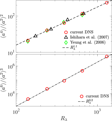
Figure 2: Normalized fourth (top) and sixth (bottom) order moments of acceleration as a function of $R_{\lambda}$.

As noted earlier, the use of multifractals is primarily motivated by Eq. (4). To get better insight, in Fig.3a, we plot $a_{0}$ and $\langle\epsilon^{3/2}\rangle/\langle\epsilon\rangle^{3/2}$ versus $R_{\lambda}$. While the latter shows a clear $R_{\lambda}^{0.14}$ scaling as anticipated from multifractals (and also the log-normal model), the former shows a steeper scaling of $R_{\lambda}^{0.25}$. An even more general and direct test is presented in Fig.3b, by checking the validity of Eq. (4) for different $p$ values. The data clearly suggest that the acceleration intermittency, being stronger, cannot be described by extending the Eulerian intermittency of the dissipation-rate. In fact, a similar observation has been made for Lagrangian velocity structure functions, where extensions of the $p$-model and the She-Leveque model severely underpredicts their intermittency (i.e., overpredicts the inertial-range exponents) Sawford and Yeung (2015).

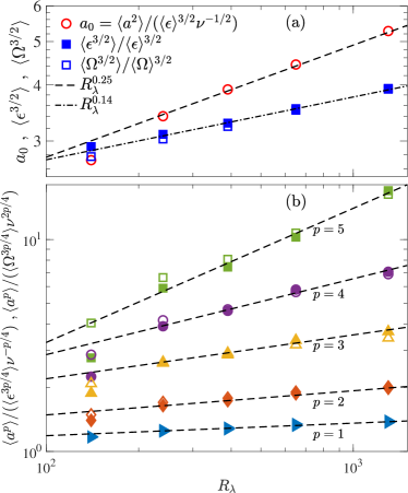
Figure 3: (a) Scaling of $a_{0}$, $\langle\epsilon^{3/2}\rangle$ and $\langle\Omega^{3/2}\rangle$. For clarity, data for $\epsilon$ and $\Omega$ are shifted up by a factor of $2$ and $1.5$ respectively. (b) Scaling of $p$-th moments of acceleration normalized by moments of $\epsilon^{3p/4}$ (filled symbols) and $\Omega^{3p/4}$ (open symbols). For clarity, data for $p=1$-$5$ are respectively shifted by factors of 1, 0.75, 0.5, 0.25, 0.12 for $\epsilon$ and 0.94, 1.01, 1.2, 1.35, 1.6 for $\Omega$.

It is worth considering if one might describe the scaling of acceleration moments in terms of enstrophy $\Omega=|\bm{\omega}|^{2}$ ($\bm{\omega}$ being the vorticity), instead of dissipation. This change addresses the likelihood that acceleration is influenced more by transverse velocity gradients than by longitudinal ones Arnéodo et al. (2008); Lanotte et al. (2013). In isotropic turbulence $\langle\Omega\rangle=\langle\epsilon\rangle/\nu$, but the higher moments differ; enstrophy being more intermittent Buaria et al. (2019); Buaria and Pumir (2022). The resulting modification to Eq. (4) is: $\langle a^{p}\rangle\sim\langle\Omega^{3p/4}\nu^{2p/4}$. However, as tested in Fig. 3a,b, the differences arise only for large $p$; even then, it is not sufficient to explain the stronger intermittency of acceleration (also see Supplementary sup ).

Acceleration variance from fourth-order structure function:

A statistical model for acceleration variance is now obtained using a methodology similar to that proposed by Hill (2002), but differing in some crucial aspects. From Eq. (1), acceleration variance can be obtained directly as

$$\langle|\mathbf{a}|^{2}\rangle=\langle|\nabla p|^{2}\rangle+\nu^{2}\langle|\nabla^{2}u|^{2}\rangle\ .$$ (8)

The viscous contribution is known to be small and can be ignored Vedula and Yeung (1999). An exact relation for variance of pressure-gradient is also known Monin and Yaglom (1975); Hill and Wilczak (1995):

$$\langle|\nabla p|^{2}\rangle=\int_{r}r^{-3}[D_{1111}(r)+D_{\alpha\alpha\alpha\alpha}(r)-6D_{11\beta\beta}(r)]dr\ ,$$ (9)

where the $D$s are the fourth order longitudinal, transverse and mixed structure functions, in order. The above results can be rewritten as Hill (2002):

$$\langle|\mathbf{a}|^{2}\rangle\simeq 4H_{\chi}\int_{r}r^{-3}D_{1111}(r)dr,$$ (10)

where $H_{\chi}$ is defined by Eqs. (8)-(9). At sufficiently high $R_{\lambda}$ ($\gtrsim 200$), DNS data Vedula and Yeung (1999); Ishihara et al. (2007) confirm that $H_{\chi}\approx 0.65$ (also see Supplementary sup ). We can normalize both sides by Kolmogorov-scales to write

$$a_{0}\simeq\frac{4H_{\chi}}{3}\int_{r}\left(\frac{r}{\eta_{K}}\right)^{-3}\frac{D_{1111}(r)}{u_{K}^{4}}d\left(\frac{r}{\eta_{K}}\right)\ .$$ (11)

Assuming standard scaling regimes Frisch (1995), we can write

$$\frac{D_{1111}(r)}{u_{K}^{4}}=\begin{cases}\frac{F}{225}\left(\frac{r}{\eta_{K}}\right)^{4}\ \ \ \ \ \ &r<\ell\ ,\\ C_{4}\left(\frac{r}{\eta_{K}}\right)^{\xi_{4}}\ \ \ \ \ \ &\ell<r<L\ ,\\ C\ \ \ \ \ \ \ &r>L\ ,\end{cases}$$ (12)

where $F$ is the flatness of $\partial u/\partial x$, $\xi_{4}$ is the inertial-range exponent, and $C_{4}$, $C$ are constants which depend on $R_{\lambda}$; $\ell$ is a crossover scale between the viscous and inertial range and is determined by matching the two regimes as

$$(F/225)({\ell}/{\eta_{K}})^{4}=C_{4}({\ell}/{\eta_{K}})^{\xi_{4}}\ .$$ (13)

Now, taking

$$F\sim R_{\lambda}^{\alpha}\ ,\ \ \ \ \ C_{4}\sim R_{\lambda}^{\beta}\ ,$$ (14)

we have

$${\ell}/{\eta_{K}}\sim R_{\lambda}^{(\beta-\alpha)/(4-\xi_{4})}\ .$$ (15)

Finally, from piecewise integration of Eq. (11), it can be shown that (see Supplementary Material sup for intermediate steps):

$$a_{0}\sim F(\ell/\eta_{K})^{2}$$ (16)

Substituting the $R_{\lambda}$-dependencies, we get

$$a_{0}\sim R_{\lambda}^{(2\alpha-\alpha\xi_{4}+2\beta)/(4-\xi_{4})}\ .$$ (17)

The values of $\alpha$, $\beta$ and $\xi_{4}$ are in principle obtainable from Eulerian intermittency models. The exponent $\alpha$ simply corresponds to $\tau_{2}$ in Eq. (6), since $F\sim\langle\epsilon^{2}\rangle/\langle\epsilon\rangle^{2}$. Multifractal and log-normal models predict $\alpha=\tau_{2}\approx 0.38$. The DNS data for $F$ are shown in Fig. 4a, giving $\alpha\approx 0.387$, in excellent agreement with the prediction, and also with previous experimental and DNS results in literature Gylfason et al. (2004); Ishihara et al. (2007).

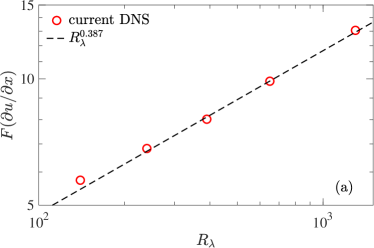
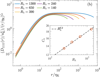
Figure 4: (a) Flatness of longitudinal velocity gradient as a function of $R_{\lambda}$. (b) Fourth-order structure function compensated by its inertial-range scaling. The inset shows the variation of coefficient $C_{4}$ in Eq. (12) as a function of $R_{\lambda}$.

On the other hand, intermittency models predict $\xi_{4}\approx 1.28$ She and Leveque (1994). Our DNS shows $\xi_{4}\approx 1.3$, which is well within statistical error bounds. Finally, the prediction for $\beta$ from multifractal model is $\beta\approx(4-3\xi_{4})/2$, which reduces to $\beta\approx\mu/3$ for log-normal model; both predictions give $\beta\approx 0.08$ (also see Supplementary sup ). Figure 4b shows the normalized fourth-order structure function from our DNS data, using $\xi_{4}\approx 1.3$. Note, as expected, the inertial-range increases with $R_{\lambda}$. The inset of the bottom panel shows $C_{4}$, giving $\beta\approx 0.2$. This observed $\beta$ is substantially larger than $0.08$ anticipated from multifractal and log-normal models.

The use of $\alpha=0.387$, $\beta=0.2$ and $\xi_{4}=1.3$ in Eq. (17) leads to

$$a_{0}\sim R_{\lambda}^{\chi},\ \ \ \chi=\zeta_{2}\approx 0.25\ ,$$ (18)

which is in excellent agreement with the high-$R_{\lambda}$ data shown in Figs. 1 and 3a. The exponent $0.25$ is virtually insensitive to a small variation in $\xi_{4}$, but is significantly impacted by the choice of $\beta=0.2$ (instead of $0.08$). Moreover, the use of $\beta\approx 0.08$ in Eq. (17) gives $a_{0}\sim R_{\lambda}^{0.15}$, which is essentially the same as the exponent $0.14$ obtained earlier in Table 1. This shows the robustness of piecewise integration leading to the result in Eq. (17) and also suggests that the discrepancy from multifractal prediction is due to the exponent $\beta$ (and hence the proportionality constant $C_{4}$). In this regard, the role of $\beta$ needs to be further explored, especially in relation to the inadequacy of Eq. (4).

We note that the exponent $0.25$ was also suggested by Hill Hill (2002). However, Hill arrived at this result by deriving that $a_{0}\sim F^{0.79}$ and $F\sim R_{\lambda}^{0.31}$ based on Antonia et al. (1981); evidently, the current data do not agree with both of these results. It appears that the two errors fortuitously cancelled out each other to give the $0.25$ exponent. Finally, we point out that the exponent $0.25$ describes the data for $R_{\lambda}\gtrsim 200$. To describe the data at lower $R_{\lambda}$, an empirical interpolation formula in the spirit of Eq. (3) can be devised with $\chi=0.25$. Least-square fit gives $c_{1}\approx 0.89$, $c_{2}\approx 40$ (also see Supplementary sup ).

Conclusions:

The moments of Lagrangian acceleration are known to deviate from classical K41 phenomenology due to intermittency. Attempts were made to quantify these deviations by extending the Eulerian multifractal models to the Lagrangian viewpoint and devising an ad-hoc interpolation formula to agree with available data from DNS and experiments. The first contribution of this article is to present new very well resolved DNS data on Lagrangian acceleration at higher $R_{\lambda}$, and show that they disagree with the results from multifractal models, and the interpolation formula. The disagreement gets increasingly stronger with the moment order. As a second contribution, the article devises a statistical model that is able to correctly capture the scaling of acceleration variance. While this framework does not seem amenable for generalization to higher-order moments, our results show that the intermittency of Lagrangian quantities remains an open problem, even more compellingly than before.

References

- La Porta et al. (2001) A. La Porta, G. A. Voth, A. M. Crawford, J. Alexander, and E. Bodenschatz, “Fluid particle accelerations in fully developed turbulence,” Nature 409, 1017–1019 (2001).
- Toschi and Bodenschatz (2009) F. Toschi and E. Bodenschatz, “Lagrangian properties of particles in turbulence,” Annu. Rev. Fluid Mech. 41, 375–404 (2009).
- Stelzenmuller et al. (2017) N. Stelzenmuller, J. I. Polanco, L. Vignal, I. Vinkovic, and N. Mordant, “Lagrangian acceleration statistics in a turbulent channel flow,” Phys. Rev. Fluids 2, 054602 (2017).
- Buaria et al. (2020a) D. Buaria, A. Pumir, F. Feraco, R. Marino, A. Pouquet, D. Rosenberg, and L. Primavera, “Single-particle Lagrangian statistics from direct numerical simulations of rotating-stratified turbulence,” Phys. Rev. Fluids 5, 064801 (2020a).
- Sawford (1991) B. L. Sawford, “Reynolds number effects in Lagrangian stochastic models of turbulent dispersion,” Phys. Fluids A 3, 1577–1586 (1991).
- Wyngaard (1992) J. C. Wyngaard, “Atmospheric turbulence,” Annu. Rev. Fluid Mech. 24, 205–234 (1992).
- Pope (1994) S. B Pope, “Lagrangian pdf methods for turbulent flows,” Annu. Rev. Fluid Mech. 26, 23–63 (1994).
- Wilson and Sawford (1996) J. D. Wilson and B. L. Sawford, “Review of Lagrangian stochastic models for trajectories in the turbulent atmosphere,” (1996).
- Kolmogorov (1941) A. N. Kolmogorov, “Local structure of turbulence in an incompressible fluid for very large Reynolds numbers,” Dokl. Akad. Nauk. SSSR 30, 299–303 (1941).
- Heisenberg (1948) W Heisenberg, “Zur statistichen Theorie der Turbulenz,” Z Phys 124, 628–657 (1948).
- Yaglom (1949) A. M. Yaglom, “On the acceleration field in a turbulent flow,” C. R. Akad. Nauk. URSS 67, 795–798 (1949).
- Yeung and Pope (1989) P. K. Yeung and S. B. Pope, “Lagrangian statistics from direct numerical simulations of isotropic turbulence,” J. Fluid Mech. 207, 531–586 (1989).
- Vedula and Yeung (1999) P. Vedula and P. K. Yeung, “Similarity scaling of acceleration and pressure statistics in numerical simulations of isotropic turbulence,” Phys Fluids 11, 1208–1220 (1999).
- Gotoh and Rogallo (1999) T. Gotoh and R. S. Rogallo, “Intermittency and scaling of pressure at small scales in forced isotropic turbulence,” J. Fluid Mech. 396, 257–285 (1999).
- Voth et al. (2002) G. A. Voth, A. La Porta, A. M. Crawford, J. Alexander, and E. Bodenschatz, “Measurement of particle accelerations in fully developed turbulence,” J. Fluid Mech. 469, 121–160 (2002).
- Sawford et al. (2003) B. L. Sawford, P. K. Yeung, M. S. Borgas, P. Vedula, A. La Porta, A. M. Crawford, and E. Bodenschatz, “Conditional and unconditional acceleration statistics in turbulence,” Phys. Fluids 15, 3478–3489 (2003).
- Mordant et al. (2004) N. Mordant, E. Lévêque, and J.-F. Pinton, “Experimental and numerical study of the Lagrangian dynamics of high reynolds turbulence,” New J. Phys. 6, 116 (2004).
- Gylfason et al. (2004) A. Gylfason, S. Ayyalasomayajula, and Z. Warhaft, “Intermittency, pressure and acceleration statistics from hot-wire measurements in wind-tunnel turbulence,” J. Fluid Mech. 501, 213–229 (2004).
- Yeung et al. (2006) P. K. Yeung, S. B. Pope, A. G. Lamorgese, and D. A. Donzis, “Acceleration and dissipation statistics of numerically simulated isotropic turbulence,” Physics of fluids 18, 065103 (2006).
- Ishihara et al. (2007) T. Ishihara, Y. Kaneda, M. Yokokawa, K. Itakura, and A. Uno, “Small-scale statistics in high resolution of numerically isotropic turbulence,” J. Fluid Mech. 592, 335–366 (2007).
- Hill (2002) R. J. Hill, “Scaling of acceleration in locally isotropic turbulence,” J. Fluid Mech. 452, 361–370 (2002).
- Reynolds (2003) A. M. Reynolds, “Superstatistical mechanics of tracer-particle motions in turbulence,” Phys. Rev. Lett. 91, 084503 (2003).
- Beck (2007) C. Beck, “Statistics of three-dimensional Lagrangian turbulence,” Phys. Rev. Lett. 98, 064502 (2007).
- Bentkamp et al. (2019) L. Bentkamp, C. C. Lalescu, and M. Wilczek, “Persistent accelerations disentangle Lagrangian turbulence,” Nat. Commun. 10, 1–8 (2019).
- Borgas (1993) M. S. Borgas, “The multifractal Lagrangian nature of turbulence,” Philos. Trans. R. Soc. A 342, 379–411 (1993).
- Chevillard et al. (2003) L. Chevillard, S. G. Roux, E. Lévêque, N. Mordant, J.-F. Pinton, and A. Arnéodo, “Lagrangian velocity statistics in turbulent flows: Effects of dissipation,” Phys. Rev. Lett. 91, 214502 (2003).
- Biferale et al. (2004) L. Biferale, G. Boffetta, A. Celani, B. J. Devenish, A. Lanotte, and F. Toschi, “Multifractal statistics of Lagrangian velocity and acceleration in turbulence,” Phys. Rev. Lett. 93, 064502 (2004).
- Sreenivasan and Antonia (1997) K. R. Sreenivasan and R. A. Antonia, “The phenomenology of small-scale turbulence,” Annu. Rev. Fluid Mech. 29, 435–77 (1997).
- Frisch (1995) U. Frisch, Turbulence: the legacy of Kolmogorov (Cambridge University Press, Cambridge, 1995).
- Ishihara et al. (2009) T. Ishihara, T. Gotoh, and Y. Kaneda, “Study of high-Reynolds number isotropic turbulence by direct numerical simulations,” Ann. Rev. Fluid Mech. 41, 165–80 (2009).
- Rogallo (1981) R. S. Rogallo, “Numerical experiments in homogeneous turbulence,” NASA Technical Memo (1981).
- Buaria et al. (2019) D. Buaria, A. Pumir, E. Bodenschatz, and P. K. Yeung, “Extreme velocity gradients in turbulent flows,” New J. Phys. 21, 043004 (2019).
- Buaria and Sreenivasan (2020) D. Buaria and K. R. Sreenivasan, “Dissipation range of the energy spectrum in high Reynolds number turbulence,” Phys. Rev. Fluids 5, 092601(R) (2020).
- Buaria et al. (2020b) D. Buaria, E. Bodenschatz, and A. Pumir, “Vortex stretching and enstrophy production in high Reynolds number turbulence,” Phys. Rev. Fluids 5, 104602 (2020b).
- Buaria et al. (2020c) D. Buaria, A. Pumir, and E. Bodenschatz, “Self-attenuation of extreme events in Navier-Stokes turbulence,” Nat. Commun. 11, 5852 (2020c).
- Buaria and Pumir (2021) D. Buaria and A. Pumir, “Nonlocal amplification of intense vorticity in turbulent flows,” Phys. Rev. Research 3, 042020 (2021).
- Buaria et al. (2022) D. Buaria, A. Pumir, and E. Bodenschatz, “Generation of intense dissipation in high Reynolds number turbulence,” Philos. Trans. R. Soc. A 380, 20210088 (2022).
- Note (1) Due to resolution concerns, we only use series 2 data from Ishihara et al. (2007), corresponding to .
- Lawson et al. (2018) J. M. Lawson, E. Bodenschatz, C. C. Lalescu, and M. Wilczek, “Bias in particle tracking acceleration measurement,” Experiments in Fluids 59, 1–14 (2018).
- Buaria et al. (2015) D. Buaria, B. L. Sawford, and P. K. Yeung, “Characteristics of backward and forward two-particle relative dispersion in turbulence at different Reynolds numbers,” Phys. Fluids 27, 105101 (2015).
- Buaria et al. (2016) D. Buaria, P. K. Yeung, and B. L. Sawford, “A Lagrangian study of turbulent mixing: forward and backward dispersion of molecular trajectories in isotropic turbulence,” J. Fluid Mech. 799, 352–382 (2016).
- Buaria and Yeung (2017) D. Buaria and P. K. Yeung, “A highly scalable particle tracking algorithm using partitioned global address space (PGAS) programming for extreme-scale turbulence simulations,” Comput. Phys. Commun. 221, 246 – 258 (2017).
- Note (2) This data is at somewhat lower resolution of , which does not effect the variance, but errors for higher-order moments are significant.
- (44) “see Supplementary material for additional details,” .
- Meneveau and Sreenivasan (1991) C. Meneveau and K. R. Sreenivasan, “The multifractal nature of turbulent energy dissipation,” J. Fluid Mech. 224, 429––484 (1991).
- Sreenivasan (1984) K. R. Sreenivasan, “On the scaling of the turbulence energy dissipation rate,” Phys. Fluids 27, 1048–1051 (1984).
- Meneveau and Sreenivasan (1987) C. Meneveau and K. R. Sreenivasan, “Simple multifractal cascade model for fully developed turbulence,” Phys. Rev. Lett. 59, 1424 (1987).
- Note (3) Note, this result corresponds to absolute moments, since we only considered the magnitude, but the odd moments of acceleration components are identically zero from symmetry.
- She and Leveque (1994) Z.-S. She and E. Leveque, “Universal scaling laws in fully developed turbulence,” Phys. Rev. Lett. 72, 336–339 (1994).
- Kolmogorov (1962) A. N. Kolmogorov, “A refinement of previous hypotheses concerning the local structure of turbulence in a viscous incompressible fluid at high Reynolds number,” J. Fluid Mech. 13, 82–85 (1962).
- Sreenivasan and Kailasnath (1993) K. R. Sreenivasan and P. Kailasnath, “An update on the intermittency exponent in turbulence,” Phys. Fluids A: Fluid Dynamics 5, 512–514 (1993).
- Buaria and Sreenivasan (2022) D. Buaria and K. R. Sreenivasan, “Intermittency of turbulent velocity and scalar fields using 3D local averaging,” arXiv:2204.08132 (2022).
- Sawford and Yeung (2015) B. L. Sawford and P. K. Yeung, “Direct numerical simulation studies of Lagrangian intermittency in turbulence,” Phys. Fluids 27, 065109 (2015).
- Arnéodo et al. (2008) A. Arnéodo et al., “Universal intermittent properties of particle trajectories in highly turbulent flows,” Phys. Rev. Lett. 100, 254504 (2008).
- Lanotte et al. (2013) A.S. Lanotte, L. Biferale, G. Boffetta, and F. Toschi, “A new assessment of the second-order moment of lagrangian velocity increments in turbulence,” J. Turb. 14, 34 (2013).
- Buaria and Pumir (2022) D. Buaria and A. Pumir, “Vorticity-strain rate dynamics and the smallest scales of turbulence,” Phys. Rev. Lett. 128, 094501 (2022).
- Note (4) The forcing term has negligible contribution to acceleration moments. This is also reaffirmed by collapse of data in Fig. 1 from various sources that use different forcings.
- Monin and Yaglom (1975) A. S. Monin and A. M. Yaglom, Statistical Fluid Mechanics, Vol. 2 (MIT Press, 1975).
- Hill and Wilczak (1995) R. J. Hill and J. M. Wilczak, “Pressure structure functions and spectra for locally isotropic turbulence,” J. Fluid Mech. 296, 247–269 (1995).
- Antonia et al. (1981) R. A. Antonia, A. J. Chambers, and B. R. Satyaprakash, “Reynolds number dependence of high-order moments of the streamwise turbulent velocity derivative,” Bound.-Layer Meteorol. 21, 159 (1981).