A Galerkin FE method for elliptic optimal control problem governed by 2D space-fractional PDEs

Abstract

In this paper, we propose a Galerkin finite element method for the elliptic optimal control problem governed by the Riesz space-fractional PDEs on 2D domains with control variable being discretized by variational discretization technique. The optimality condition is derived and priori error estimates of control, costate and state variables are successfully established. Numerical test is carried out to illustrate the accuracy performance of this approach.

1 Introduction

The optimal control problems (OCPs) governed by fractional partial differential equations (PDEs) forms a new branch in the area of optimal control, which recently have gained explosive interest and enjoy great potential in the applications as diverse as temperature control, environmental engineering, crystal growth, disease transmission and so forth [11, 12].

In this study, we consider the distributed quadratic fractional OCPs:

$$\min\limits_{q\in\mathscr{K}}J(u,q):=\frac{1}{2}||u(x,y)-u_{d}(x,y)||^{2}_{L^{2}(\Omega)}+\frac{\gamma}{2}||q(x,y)||^{2}_{L^{2}(\Omega)},$$ (1.1)

subjected to the 2D elliptic Riesz fractional PDEs

$$\left\{\begin{array}[]{lll}\displaystyle\kappa_{1}\frac{\partial^{\alpha}u(x,y)}{\partial|x|^{\alpha}}+\kappa_{2}\frac{\partial^{\alpha}u(x,y)}{\partial|y|^{\alpha}}=g(x,y)+q(x,y),\quad(x,y)\in\Omega,\\ u(x,y)=0,\quad(x,y)\in\partial\Omega,\end{array}\right.$$ (1.4)

where $\Omega=(a,b)\times(c,d)$, $\kappa_{1},\ \kappa_{2},\ \gamma\in\mathbb{R}^{+}$, $1<\alpha<2$, $\mathscr{K}$ is a closed convex set and $u_{d}(x,y)$ is the desired state. The fractional derivatives have the weakly singular convolution form:

$$\frac{\partial^{\alpha}u(x,y)}{\partial|x|^{\alpha}}=\frac{-1}{2\cos(\frac{\pi\alpha}{2})}\Big{\{}{{}_{a}^{L}D^{\alpha}_{x}}u(x,y)+^{R}_{x}D^{\alpha}_{b}u(x,y)\Big{\}},$$

$${}^{L}_{a}D^{\alpha}_{x}u(x,y)=\frac{1}{\Gamma(2-{\alpha})}\frac{d^{2}}{dx^{2}}\int^{x}_{a}(x-\omega)^{1-{\alpha}}u(\omega,y)d\omega,$$

$${}^{R}_{x}D^{\alpha}_{b}u(x,y)=\frac{1}{\Gamma(2-{\alpha})}\frac{d^{2}}{dx^{2}}\int^{b}_{x}(\omega-x)^{1-{\alpha}}u(\omega,y)d\omega,$$

and so is $\frac{\partial^{\alpha}u(x,y)}{\partial|y|^{\alpha}}$ with regard to $y$.

In the past decades, the OCPs governed by PDEs have been widely investigated and a large collection of works on their numerical algorithms have been done, which cover spectral method [17], FE method [3, 8, 7, 18], mixed FE method [4, 5], least square method [16], variational discretization method [10, 13] and some other niche methods. However, the discussions on fractional OCPs have been rarely reported. The difficulty consisting in finding their numerical solutions not only lies in the nonsmoothness caused by the inequality constraints on control or state, but also the vectorial convolution in fractional derivatives, which bring enormous challenge in the endeavor of numerical schemes and theoretical analysis. Hence, it is of great significance to study the numerical methods for fractional OCPs. In [14], Mophou studied the first-order optimality condition for the OCPs governed by time-fractional diffusion equations. In [19], Ye and Xu derived the optimality condition for the time-fractional OCPs with state integral constraint and developed a spectral method. Zhou and Gong proposed a fully discrete FE scheme to solve the time-fractional OCPs [21]. Du et al. combined the finite difference method and gradient projection algorithm to obtain a fast scheme for the OCPs governed by space-fractional PDEs [6]. Zhou and Tan addressed a fully discrete FE scheme for the space-fractional OCPs [22]. Zhang et al. proposed the space-time discontinuous Galerkin FE methods for the time-fractional OCPs [20, 23]. Gunzburger and Wang proposed a fully discrete FE scheme along with convolution quadrature for the time-fractional OCPs [9]. However, these works are limited to 1D or time-fractional OCPs. Due to the difficulty in constructing algorithm and theoretical analysis, there is no study reported on multi-dimensional space-fractional OCPs. Inspired by this, we propose a Galerkin FE scheme for the elliptic OCPs governed by 2D space-fractional PDEs, where the control variable is discretized by variational discretization technique because the inequality constraints always lead to low regularity. The first-order optimality condition is derived and the priori error estimates for the control, costate and state variables are rigorously analyzed.

The rest of this paper are organized as follows. In Section 2, we derive the first-order optimality condition for Eqs. (1.1)-(1.4) and in Secton 3, we propose a fully discrete FE scheme for the optimality system. In Section 4, we establish the priori error estimates for the control, costate and state and finally, numerical tests are included to confirm our results.

2 Optimality condition

To begin with, we define $H^{\mu}_{0}(\Omega)$ by the closure in $C^{\infty}_{0}(\Omega)$ with respect to the fractional Sobolev norm $||\cdot||_{H^{\mu}(\Omega)}$ defined by $||u||_{H^{\mu}(\Omega)}=\big{(}||u||^{2}_{L^{2}(\Omega)}+|u|^{2}_{H^{\mu}(\Omega)}\big{)}^{1/2}$, $|u|_{H^{\mu}(\Omega)}=||\ |\boldsymbol{\omega}|^{\mu}\mathcal{F}[\tilde{u}]||_{L^{2}(\Omega)}$ with $1<\mu<2$ and $\mathcal{F}[\tilde{u}]$ being the Fourier transform of zero extension of $u$ outside $\Omega$.

Consider the model of the 2D space-fractional OCPs:

$$\textrm{Minimize}\ J(u,q)\ \textrm{subjected to Eq.}\ (\ref{eq02}),\quad(q,u)\in\mathscr{K}\times L^{2}(\Omega),$$ (2.5)

with the pointwise constraints on control variable, i.e.,

$$\mathscr{K}=\{q\in L^{2}(\Omega):\ v_{1}\leq q(x,y)\leq v_{2}\ \textrm{a.e. in}\ \Omega,\ v_{1},\ v_{2}\in\mathbb{R}\}.$$

Lemma 2.1.

[15] If $1<\mu<2$, $u,\ \chi\in H_{0}^{\mu}(\Omega)$, then we have

$$({{}^{L}_{a}}D_{x}^{\mu}u,\chi)=({{}^{L}_{a}}D_{x}^{\frac{\mu}{2}}u,{{}^{R}_{x}}D_{b}^{\frac{\mu}{2}}\chi),\quad({{}^{R}_{x}}D_{b}^{\mu}u,\chi)=({{}^{R}_{x}}D_{b}^{\frac{\mu}{2}}u,{{}^{L}_{a}}D_{x}^{\frac{\mu}{2}}\chi),$$

and the similar results exist for the fractional derivatives in $y$-direction.

Theorem 2.1.

The fractional OCPs (2.5) have a unique pair $(q,u)$ and there is a costate state $p$ such that the triplet $(q,p,u)$ fulfills the first-order optimality condition as follow:

$$\left\{\begin{array}[]{lll}\displaystyle\kappa_{1}\frac{\partial^{\alpha}u(x,y)}{\partial|x|^{\alpha}}+\kappa_{2}\frac{\partial^{\alpha}u(x,y)}{\partial|y|^{\alpha}}=g(x,y)+q(x,y),\quad(x,y)\in\Omega,\\ u(x,y)=0,\quad(x,y)\in\partial\Omega,\end{array}\right.$$ (2.8)

$$\left\{\begin{array}[]{lll}\displaystyle\kappa_{1}\frac{\partial^{\alpha}p(x,y)}{\partial|x|^{\alpha}}+\kappa_{2}\frac{\partial^{\alpha}p(x,y)}{\partial|y|^{\alpha}}=u(x,y)-u_{d}(x,y),\quad(x,y)\in\Omega,\\ p(x,y)=0,\quad(x,y)\in\partial\Omega,\end{array}\right.$$ (2.11)

$$\int_{\Omega}(\gamma q+p)(\delta q-q)dxdy\geq 0,\quad\forall\delta q\in\mathscr{K}.$$ (2.12)

Proof.

Due to the strictly convex $J(\cdot,\cdot)$, we easily know that the OCPs (2.5) admit a unique pair $(q,u)$ by standard arguments. Next, we prove the first-order optimality condition (2.8)-(2.12). Suppose that $v(x,y)$ is the state with respect to $\delta q(x,y)-q(x,y)$, i.e.,

$$\left\{\begin{array}[]{lll}\displaystyle\kappa_{1}\frac{\partial^{\alpha}v(x,y)}{\partial|x|^{\alpha}}+\kappa_{2}\frac{\partial^{\alpha}v(x,y)}{\partial|y|^{\alpha}}=\delta q(x,y)-q(x,y),\quad(x,y)\in\Omega,\\ v(x,y)=0,\quad(x,y)\in\partial\Omega.\end{array}\right.$$ (2.15)

Define the reduced cost functional $\hat{J}(q):=J(q,u(q))$, which maps $q$ from $\mathscr{K}$ to $\mathbb{R}$. Then the first-order optimality condition reads as

$$\hat{J}^{\prime}(q)(\delta q-q)\geq 0,\quad\forall\delta q\in\mathscr{K}.$$

which leads to

$$\int_{\Omega}\gamma q(\delta q-q)dxdy+\int_{\Omega}v(u-u_{d})dxdy\geq 0,\quad\forall\delta q\in\mathscr{K}.$$ (2.16)

On the other hand, we present the adjoint state equation

$$\left\{\begin{array}[]{lll}\displaystyle\kappa_{1}\frac{\partial^{\alpha}p(x,y)}{\partial|x|^{\alpha}}+\kappa_{2}\frac{\partial^{\alpha}p(x,y)}{\partial|y|^{\alpha}}=u(x,y)-u_{d}(x,y),\quad(x,y)\in\Omega,\\ p(x,y)=0,\quad(x,y)\in\partial\Omega,\end{array}\right.$$ (2.19)

with the costate $p$. Multiplying by $v$ and using Lemma 2.1, there holds

$$\int_{\Omega}v(u-u_{d})dxdy =\kappa_{1}\int_{\Omega}v\cdot\frac{\partial^{\alpha}p(x,y)}{\partial|x|^{\alpha}}dxdy+\kappa_{2}\int_{\Omega}v\cdot\frac{\partial^{\alpha}p(x,y)}{\partial|y|^{\alpha}}dxdy$$

$$=\frac{-\kappa_{1}}{2\cos(\frac{\pi\alpha}{2})}\int_{\Omega}{{}_{a}^{L}D^{\alpha}_{x}}p\cdot v+^{R}_{x}D^{\alpha}_{b}p\cdot vdxdy-\frac{\kappa_{2}}{2\cos(\frac{\pi\alpha}{2})}\int_{\Omega}{{}_{c}^{L}D^{\alpha}_{y}}p\cdot v+^{R}_{y}D^{\beta}_{d}p\cdot vdxdy$$

$$=\frac{-\kappa_{1}}{2\cos(\frac{\pi\alpha}{2})}\int_{\Omega}p\cdot^{R}_{x}D^{\alpha}_{b}v+p\cdot{{}_{a}^{L}D^{\alpha}_{x}}vdxdy-\frac{\kappa_{2}}{2\cos(\frac{\pi\alpha}{2})}\int_{\Omega}p\cdot^{R}_{y}D^{\alpha}_{d}v+p\cdot{{}_{c}^{L}D^{\alpha}_{y}}vdxdy$$

$$=\kappa_{1}\int_{\Omega}p\cdot\frac{\partial^{\alpha}v(x,y)}{\partial|x|^{\alpha}}dxdy+\kappa_{2}\int_{\Omega}p\cdot\frac{\partial^{\alpha}v(x,y)}{\partial|y|^{\alpha}}dxdy.$$

Combing with Eq. (2.15), we obtain

$$\int_{\Omega}v(u-u_{d})dxdy=\int_{\Omega}p(\delta q-q)dxdy,$$ (2.20)

and substituting Eq. (2.20) into (2.16) finally leads to the above results. ∎

3 Fully discrete Galerkin FE scheme

In order to derive the FE scheme, divide $\Omega$ by triangle meshes $\mathcal{T}_{h}$ and for each triangle $K$, let $h_{K}=\textrm{diam}\ K$ and $h=\max\limits_{K\in\mathcal{T}_{h}}h_{K}$. Define the FE subspace $\mathcal{V}_{h}=\{v:v|_{K}\in P_{linear},\ \forall K\in\mathcal{T}_{h}\}$ and $\mathcal{V}_{h}\in H^{\frac{\alpha}{2}}_{0}(\Omega)$, where $P_{linear}$ is the linear polynomial space. Using fractional variational principle, the FE scheme for state Eq. (1.4) is to find $u_{h}\in\mathcal{V}_{h}$ such that

$$\varLambda_{h}(u_{h},\chi_{h})=(g+q,\chi_{h}),\quad\forall\chi_{h}\in\mathcal{V}_{h},$$ (3.21)

where

$$\varLambda_{h}(u,v) =\frac{\kappa_{1}}{2\cos(\frac{\pi\alpha}{2})}\Bigg{\{}({{}^{L}_{a}}D^{\frac{\alpha}{2}}_{x}u,{{}_{x}}^{R}D^{\frac{\alpha}{2}}_{b}v)+({{}_{x}^{R}}D^{\frac{\alpha}{2}}_{b}u,{{}_{a}^{L}}D^{\frac{\alpha}{2}}_{x}v)\Bigg{\}}$$

$$\ \ +\frac{\kappa_{2}}{2\cos(\frac{\pi\alpha}{2})}\Bigg{\{}({{}_{c}^{L}}D^{\frac{\alpha}{2}}_{y}u,{{}_{y}^{R}}D^{\frac{\alpha}{2}}_{d}v)+({{}_{y}^{R}}D^{\frac{\alpha}{2}}_{d}u,{{}_{c}^{L}}D^{\frac{\alpha}{2}}_{y}v)\Bigg{\}},$$

which satisfies $\varLambda_{h}(u,v)\leq C||u||_{eng}||v||_{eng}$, $\varLambda_{h}(u,u)\geq C||u||^{2}_{eng}$ with the energy norms

$$||u||_{eng}=\big{(}||u||^{2}_{L^{2}(\Omega)}+|u|^{2}_{eng}\big{)}^{\frac{1}{2}},\quad|u|_{eng}=|\varLambda_{h}(u,u)|^{\frac{1}{2}}.$$

which is equivalent to $||u||_{H^{\frac{\alpha}{2}}}(\Omega)$ [15]. Denote the $L^{2}$ projection of $u$ by $\mathcal{R}_{h}u$ and the piecewise polynomial interpolant of $u$ by $\Pi_{h}u$, which have the below properties [1]:

$$||u-\mathcal{R}_{h}u||_{L^{2}(\Omega)} \leq Ch^{r}||u||_{H^{r}(\Omega)},$$ (3.22)

$$||u-{\Pi}_{h}u||_{H^{s}(\Omega)} \leq Ch^{r-s}||u||_{H^{r}(\Omega)},\quad 0\leq s\leq r.$$ (3.23)

In addition, we define the elliptic projection $\mathcal{P}_{h}:H_{0}^{\frac{\alpha}{2}}(\Omega)\mapsto\mathcal{V}_{h}$ by

$$\varLambda_{h}(u,\chi_{h})=\varLambda_{h}(\mathcal{P}_{h}u,\chi_{h}),\quad\forall\chi_{h}\in\mathcal{V}_{h},$$

which satisfies the following approximate property.

Lemma 3.1.

[2] Let $u\in H^{r}(\Omega)\cap\mathcal{V}_{h}$. Then we have

$$||u-\mathcal{P}_{h}u||_{H^{\frac{\alpha}{2}}(\Omega)}\leq Ch^{r-\frac{\alpha}{2}}||u||_{H^{r}(\Omega)},\ \ \alpha<2r,$$ (3.24)

with a constant $C$ independent of $h$.

We can derive the following convergent result for the above FE scheme.

Lemma 3.2.

Let $q=0$ and $u\in H_{0}^{1+\frac{\alpha}{2}}(\Omega)$. Then there exists a constant $C$ unrelated to $h$ such that

$$||u-u_{h}||_{H^{\frac{\alpha}{2}}(\Omega)}\leq Ch||u||_{H^{1+\frac{\alpha}{2}}(\Omega)}.$$ (3.25)

Proof.

Using Galerkin orthogonality, we have

$$C||u-u_{h}||_{eng} \leq\varLambda_{h}(u-u_{h},u-u_{h})=\varLambda_{h}(u-u_{h},u-\chi_{h})$$

$$\leq\bar{C}||u-u_{h}||_{eng}||u-\chi_{h}||_{eng}.$$

with $\bar{C}$ independent of $h$. Since the equivalence of $||\cdot||_{eng}$ and $||\cdot||_{H^{\frac{\alpha}{2}}(\Omega)}$, it implies that

$$||u-u_{h}||_{H^{\frac{\alpha}{2}}(\Omega)}\leq C\inf\limits_{\chi_{h}\in\mathcal{V}_{h}}||u-\chi_{h}||_{H^{\frac{\alpha}{2}}(\Omega)}.$$

Taking $\chi_{h}=\Pi_{h}u$ and noticing (3.23), we finally obtain

$$||u-u_{h}||_{H^{\frac{\alpha}{2}}(\Omega)}\leq C||u-\Pi_{h}u||_{H^{\frac{\alpha}{2}}(\Omega)}\leq Ch||u||_{H^{1+\frac{\alpha}{2}}(\Omega)},$$

which ends the proof. ∎

Letting $q\neq 0$, the FE scheme for Eqs. (1.1)-(1.4) is to find a pair $(q_{h},u_{h})$ such that

$$\textrm{Minimize}\ J(u_{h},q_{h})\ \textrm{subjected to Eq.}\ (\ref{eq12}),\quad(q_{h},u_{h})\in\mathscr{K}\times\mathcal{V}_{h},$$ (3.26)

which is equivalent to find the triplet $(q_{h},p_{h},u_{h})$ fulfilling the discrete optimality condition:

$$\left\{\begin{array}[]{lll}\displaystyle\varLambda_{h}(u_{h},\chi_{h})=(g+q_{h},\chi_{h}),\quad\forall\chi_{h}\in\mathcal{V}_{h},\\ u_{h}(x,y)=0,\quad(x,y)\in\partial\Omega,\end{array}\right.$$ (3.29)

$$\left\{\begin{array}[]{lll}\displaystyle\varLambda_{h}(p_{h},\chi_{h})=(u_{h}-u_{d},\chi_{h}),\quad\forall\chi_{h}\in\mathcal{V}_{h},\\ p_{h}(x,y)=0,\quad(x,y)\in\partial\Omega,\end{array}\right.$$ (3.32)

$$\int_{\Omega}(\gamma q_{h}+p_{h})(\delta q_{h}-q_{h})dxdy\geq 0,\quad\forall\delta q_{h}\in\mathscr{K}.$$ (3.33)

Due to the variational inequality, the control variable always has low regularity. To overcome this drawback, we use the variational discretization method to treat $q$, i.e., (3.33) is recast as

$$q_{h}=P_{\mathscr{K}}\Bigg{(}-\frac{1}{\gamma}p_{h}\Bigg{)}=\max\Bigg{\{}v_{1},\min\Bigg{(}-\frac{1}{\gamma}p_{h},v_{2}\Bigg{)}\Bigg{\}},$$ (3.34)

where $P_{\mathscr{K}}$ is termed by pointwise projection operator.

4 Error estimates

In this section, we establish the convergent analysis for the above FE scheme (3.29)-(3.34) and to this end, we introduce the auxiliary variational equations:

$$\varLambda_{h}(u_{h}(q),\chi_{h}) =(g+q,\chi_{h}),\quad\forall\chi_{h}\in\mathcal{V}_{h},$$ (4.35)

$$\varLambda_{h}(p_{h}(q),\chi_{h}) =(u_{h}(q)-u_{d},\chi_{h}),\quad\forall\chi_{h}\in\mathcal{V}_{h}.$$ (4.36)

Obviously, $u_{h}(q)$ is the FE solution of state $u$ and by Lemma 3.2, there exists

$$||u-u_{h}(q)||_{H^{\frac{\alpha}{2}}(\Omega)}\leq Ch||u||_{H^{1+\frac{\alpha}{2}}(\Omega)}.$$ (4.37)

Lemma 4.1.

If $(q,p,u)$ are the analytical solutions of the OCPs (2.5), $(q_{h},p_{h},u_{h})$ are the FE solutions obtained by (3.29)-(3.34) and $q\in H^{1}(\Omega)$, then we have

$$||q-q_{h}||_{L^{2}(\Omega)}\leq Ch+C||p-p_{h}(q)||_{L^{2}(\Omega)},$$ (4.38)

where $C$ is a constant unrelated to $h$.

Proof.

Using Eqs. (3.29)-(3.32) and Eqs. (4.35)-(4.36), we find

$$(q-q_{h},\chi_{h}) =\Lambda_{h}(u_{h}(q)-u_{h},\chi_{h}),$$

$$(u_{h}(q)-u_{h},\chi^{*}_{h}) =\Lambda_{h}(p_{h}(q)-p_{h},\chi^{*}_{h}),\quad\forall\chi_{h},\ \chi^{*}_{h}\in\mathcal{V}_{h},$$

and letting $\chi_{h}=p_{h}(q)-p_{h}$, $\chi^{*}_{h}=u_{h}(q)-u_{h}$ leads to

$$(q-q_{h},p_{h}(q)-p_{h})=(u_{h}(q)-u_{h},u_{h}(q)-u_{h})\geq 0.$$

From the above inequality, it follows that

$$\gamma||q-q_{h}||^{2}_{L^{2}(\Omega)} =(\gamma q+p_{h}(q),q-q_{h})-(\gamma q_{h}+p_{h},q-q_{h})-(p_{h}(q)-p_{h},q-q_{h})$$

$$\leq(\gamma q+p_{h}(q),q-q_{h})-(\gamma q_{h}+p_{h},q-q_{h})$$

$$\leq(\gamma q+p,q-q_{h})+(p_{h}(q)-p,q-q_{h})$$

$$\quad-(\gamma q_{h}+p_{h},q-\mathcal{R}_{h}q)+(\gamma q_{h}+p_{h},q_{h}-\mathcal{R}_{h}q).$$

Meanwhile, by virtue of (2.12) and (3.33), we have

$$(\gamma q+p,q-q_{h})\leq 0,\quad(\gamma q_{h}+p_{h},q_{h}-\mathcal{R}_{h}q)\leq 0,$$

and then it suffices to prove that

$$\begin{aligned} \gamma||q-q_{h}||^{2}_{L^{2}(\Omega)}&\leq(p_{h}(q)-p,q-q_{h})-(\gamma q_{h}+p_{h},q-\mathcal{R}_{h}q)\\ &=(p_{h}(q)-p,q-q_{h})+\gamma(q-q_{h},q-\mathcal{R}_{h}q)+(p-p_{h}(q),q-\mathcal{R}_{h}q)\\ &\quad+(p_{h}(q)-p_{h},q-\mathcal{R}_{h}q)-(\gamma q+p,q-\mathcal{R}_{h}q)\\ &=(p_{h}(q)-p,q-q_{h})+\gamma(q-q_{h},q-\mathcal{R}_{h}q)\\ &\quad+(p-p_{h}(q),q-\mathcal{R}_{h}q)-(\gamma q+p,q-\mathcal{R}_{h}q).\end{aligned}$$ (4.39)

Furthermore, by using the properties of $\mathcal{R}_{h}$ and $q\in H^{1}(\Omega)$, there exists

$$\begin{aligned} (\gamma q+p,q-\mathcal{R}_{h}q)&=(\gamma q+p-\mathcal{R}_{h}(\gamma q+p),q-\mathcal{R}_{h}q)\\ &\leq||\gamma q+p-\mathcal{R}_{h}(\gamma q+p)||_{L^{2}(\Omega)}||q-\mathcal{R}_{h}q||_{L^{2}(\Omega)}\leq Ch^{2}.\end{aligned}$$ (4.40)

Applying (3.22), (4.40) and Young’s inequality to (4.39), we have

$$\gamma||q-q_{h}||^{2}_{L^{2}(\Omega)} \leq\varepsilon||q-q_{h}||^{2}_{L^{2}(\Omega)}+C_{\varepsilon}||p-p_{h}(q)||^{2}_{L^{2}(\Omega)}$$

$$\quad+C_{\varepsilon}||q-\mathcal{R}_{h}q||^{2}_{L^{2}(\Omega)}-(\gamma q+p,q-\mathcal{R}_{h}q)$$

$$\leq\varepsilon||q-q_{h}||^{2}_{L^{2}(\Omega)}+Ch^{2}+C_{\varepsilon}||p-p_{h}(q)||^{2}_{L^{2}(\Omega)}.$$

By taking $\varepsilon<\gamma$, we finally obtain

$$||q-q_{h}||_{L^{2}(\Omega)}\leq Ch+C||p-p_{h}(q)||_{L^{2}(\Omega)},$$

and this completes the proof. ∎

To derive the error bounds, we further give the auxiliary equation

$$\varLambda_{h}(p_{h}(u),\chi_{h}) =(u-u_{d},\chi_{h}),\quad\forall\chi_{h}\in\mathcal{V}_{h},$$ (4.41)

and obviously, $p_{h}(u)$ is the FE solution of costate $p$, which satisfies

$$||p-p_{h}(u)||_{H^{\frac{\alpha}{2}}(\Omega)}\leq Ch||p||_{H^{1+\frac{\alpha}{2}}(\Omega)}.$$ (4.42)

Based on the above discussions, we have the following priori error estimates.

Theorem 4.1.

If $(q,p,u)$ are the analytical solutions of the OCPs (2.5), $(q_{h},p_{h},u_{h})$ are the FE solutions obtained by (3.29)-(3.34) and $q\in H^{1}(\Omega)$, $p,u\in H_{0}^{1+\frac{\alpha}{2}}(\Omega)$, then we have

$$||q-q_{h}||_{L^{2}(\Omega)}+||p-p_{h}||_{H^{\frac{\alpha}{2}}(\Omega)}+||u-u_{h}||_{H^{\frac{\alpha}{2}}(\Omega)}\leq Ch,$$ (4.43)

where $C$ is a constant unrelated to $h$.

Proof.

Multiplying Eq. (2.11) by $\chi_{h}\in\mathcal{V}_{h}$ and subtracting Eq. (4.36), we have

$$C||p-p_{h}(q)||^{2}_{eng} \leq\varLambda_{h}(p-p_{h}(q),p-p_{h}(q))$$

$$\leq\varLambda_{h}(p-p_{h}(q),\mathcal{P}_{h}p-p_{h}(q))+\varLambda_{h}(p-p_{h}(q),p-\mathcal{P}_{h}p)$$

$$=(u-u_{h}(q),\mathcal{P}_{h}p-p_{h}(q))$$

$$=(u-u_{h}(q),p-p_{h}(q))+(u-u_{h}(q),\mathcal{P}_{h}p-p),$$

by taking $\chi_{h}=p-p_{h}(q)$ in both two equations.

Using the equivalence of $||\cdot||_{eng}$ and $||\cdot||_{H^{\frac{\alpha}{2}}(\Omega)}$ and Lemma 3.1, there exists

$$||p-p_{h}(q)||^{2}_{H^{\frac{\alpha}{2}}(\Omega)} \leq\delta||p-p_{h}(q)||^{2}_{L^{2}(\Omega)}+C_{\delta}||u-u_{h}(q)||^{2}_{L^{2}(\Omega)}+C_{\delta}||p-\mathcal{P}_{h}p||^{2}_{H^{\frac{\alpha}{2}}}$$

$$\leq\delta||p-p_{h}(q)||^{2}_{L^{2}(\Omega)}+C_{\delta}||u-u_{h}(q)||^{2}_{L^{2}(\Omega)}+Ch^{2}||p||^{2}_{H^{1+\frac{\alpha}{2}}(\Omega)},$$

with $0<\delta\ll 1$, which implies

$$||p-p_{h}(q)||_{H^{\frac{\alpha}{2}}(\Omega)} \leq Ch||p||_{H^{1+\frac{\alpha}{2}}(\Omega)}+C||u-u_{h}(q)||_{H^{\frac{\alpha}{2}}}.$$

Combining with (4.37) and Lemma 4.1, we obtain

$$\begin{aligned} ||q-q_{h}||_{L^{2}(\Omega)}\leq Ch+C||p-p_{h}(q)||_{H^{\frac{\alpha}{2}}(\Omega)}\leq Ch+C||u-u_{h}(q)||_{L^{2}(\Omega)}\leq Ch.\end{aligned}$$ (4.44)

Subtracting Eq. (3.29) from Eq. (4.35) and taking $\chi_{h}=u_{h}(q)-u_{h}$, it holds that

$$C||u_{h}(q)-u_{h}||^{2}_{eng} \leq\varLambda_{h}(u_{h}(q)-u_{h},u_{h}(q)-u_{h})=(q-q_{h},u_{h}(q)-u_{h})$$

$$\leq||q-q_{h}||_{L^{2}(\Omega)}||u_{h}(q)-u_{h}||_{eng}.$$

Then, based on the error bound of $q-q_{h}$, we can get

$$||u_{h}(q)-u_{h}||_{H^{\frac{\alpha}{2}}(\Omega)} \leq C||q-q_{h}||_{L^{2}(\Omega)}\leq Ch,$$ (4.45)

and similarly, from the difference of Eqs. (3.32) and (4.41), it follows that

$$||p_{h}(u)-p_{h}||_{H^{\frac{\alpha}{2}}(\Omega)} \leq C||u-u_{h}||_{L^{2}(\Omega)}.$$ (4.46)

Using (4.37), (4.42), (4.45), (4.46) and triangle inequality, we obtain

$$\begin{aligned} ||u-u_{h}||_{H^{\frac{\alpha}{2}}(\Omega)}&\leq||u-u_{h}(q)||_{H^{\frac{\alpha}{2}}(\Omega)}+||u_{h}(q)-u_{h}||_{H^{\frac{\alpha}{2}}(\Omega)}\\ &\leq Ch||u||_{H^{1+\frac{\alpha}{2}}(\Omega)}+C||q-q_{h}||_{L^{2}(\Omega)}\leq Ch,\end{aligned}$$ (4.47)

$$\begin{aligned} ||p-p_{h}||_{H^{\frac{\alpha}{2}}(\Omega)}&\leq||p-p_{h}(u)||_{H^{\frac{\alpha}{2}}(\Omega)}+||p_{h}(u)-p_{h}||_{H^{\frac{\alpha}{2}}(\Omega)}\\ &\leq Ch||p||_{H^{1+\frac{\alpha}{2}}(\Omega)}+C||u-u_{h}||_{H^{\frac{\alpha}{2}}}\leq Ch.\end{aligned}$$ (4.48)

Consequently, combining (4.44), (4.47) and (4.48), we obtain the priori error estimate. ∎

5 Illustrative test

In this section, to illustrate the accuracy performance of the proposed FE scheme, numerical tests are carried out and numerical results are presented. For solving the coupled system (3.29)-(3.34), we adopt the fixed-point iterative algorithm and terminate iterative loop by reaching a solution $q_{h}$ with tolerant error 1.0e-12. We employ piecewise linear interpolation to approximate $p$, $u$ and variational discretization method to discretize $q$. Meanwhile, denote

$$Cov.\ order=\log_{2}\Bigg{(}\frac{e_{h_{1}}}{e_{h_{2}}}\Bigg{)}\Bigg{/}\log_{2}\Bigg{(}\frac{h_{1}}{h_{2}}\Bigg{)},$$

where $e_{h_{k}}$ is the global error corresponding to the meshsize $h_{k}$, $k=1,\ 2$.

Example 1. Letting $\kappa_{1}=\kappa_{2}=1$, $\gamma=1$ and $\mathscr{K}=\{q\in L^{2}(\Omega):\ -3\leq q(x,y)\leq-0.1\}$, consider the problem on $\Omega=(0,1)\times(0,1)$ with the analytic solutions

$$u =10x(1-x)y(1-y),$$

$$p =5x(1-x)y(1-y),$$

$$q =\max\big{\{}-3,\min\{-p,-0.1\}\big{\}},$$

where $g$, $u_{d}$ are determined by $u$, $p$ and $q$ via the model of OCPs.

We evaluate the global error at coarse mesh and then refine the mesh several times. In Fig. 1, we show the decline behavior of error for the control, state and adjoint state variables with different $\alpha$ in log-log scale. In Fig. 2, we present an unstructured mesh of $h=1/25$ and compare the analytic solution with the approximation of state when $\alpha=1.9$. To obtain more insight about accuracy, letting $\alpha=1.3$, we compute the error with different $h$ and report the convergent order for control, state and adjoint state variables in Table 1. From the above results, we observe that our method is almost convergent with theoretical order and yields the solution indistinguishable from the analytic solution, which confirm the convergent accuracy and theoretical analysis.

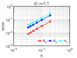
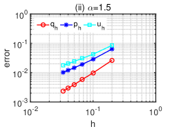
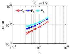
Figure 1: Evolution of error versus the change of $h$ for different $\alpha$: (i) $\alpha=1.1$; (ii) $\alpha=1.5$; (iii) $\alpha=1.9$.

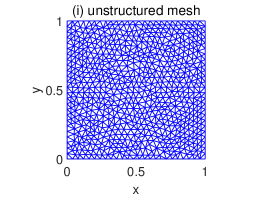
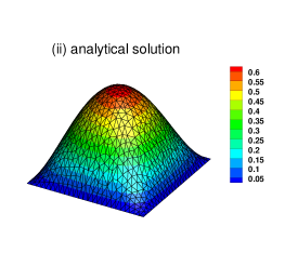
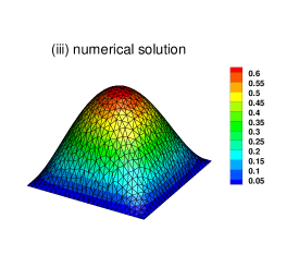
Figure 2: Unstructured triangular mesh, analytical and numerical solutions of state: (i) $h=1/25$; (ii) $u$; (iii) $u_{h}$.

Table 1: The global error and convergent order for $q_{h}$, $p_{h}$ and $u_{h}$ when $\alpha=1.3$.

$h$	$||q-q_{h}||_{L^{2}(\Omega)}$	$Cov.\ order$	$||p-p_{h}||_{H^{\frac{\alpha}{2}}(\Omega)}$	$Cov.\ order$	$||u-u_{h}||_{H^{\frac{\alpha}{2}}(\Omega)}$	$Cov.\ order$
1/10	1.4265e-02	-	4.0697e-02	-	5.8055e-02	-
1/15	8.4741e-03	1.28	2.6194e-02	1.09	3.9514e-02	0.95
1/20	5.8169e-03	1.31	1.9352e-02	1.05	3.0027e-02	0.96

Acknowledgement: This research was supported by the Natural Science Foundation of Hunan Province of China (No. 2020JJ5514) and the Scientific Research Funds of Hunan Provincial Education Department (Nos. 19C1643, 19B509 and 20B532).

References

Brenner and Scott [1994]
S.C. Brenner, L.R. Scott,
The Mathematical Theory of Finite Element Methods,
Springer, New York,
1994.
Bu et al. [2014]
W.P. Bu, Y.F. Tang, J.Y.
Yang, Galerkin finite element method for two-dimensional
Riesz space fractional diffusion equations, J. Comput.
Phys. 276 (2014) 26–38.
Chang and Yang [2008]
Y.Z. Chang, D.P. Yang,
Superconvergence analysis of finite element methods for
optimal control problems of the stationary Benard type,
J. Comput. Math. 26
(2008) 660–676.
Chen [2008]
Y.P. Chen, Superconvergence of mixed finite
element methods for optimal control problems, Math.
Comput. 77 (2008)
1269–1291.
Chen and Lu [2010]
Y.P. Chen, Z.L. Lu, Error
estimates for parabolic optimal control problem by fully discrete mixed
finite element methods, Finite Elem. Anal. Des.
46 (2010) 957–965.
Du et al. [2016]
N. Du, H. Wang, W.B. Liu,
A fast gradient projection method for a constrained
fractional optimal control, J. Sci. Comput.
68 (2016) 1–20.
Gong et al. [2014]
W. Gong, G.S. Wang, N.N.
Yan, Approximations of elliptic optimal control problems
with controls acting on a lower dimensional manifold, SIAM
J. Control. Optim. 52 (2014)
2008–2035.
Gong and Yan [2016]
W. Gong, N.N. Yan, Finite
element approximations of parabolic optimal control problems with controls
acting on a lower dimensional manifold, SIAM J. Numer.
Anal. 54 (2016)
1229–1262.
Gunzburger and Wang [2019]
M. Gunzburger, J.L. Wang,
Error analysis of fully discrete finite element
approximations to an optimal control problem governed by a time-fractional
PDE, SIAM J. Control. Optim. 57
(2019) 241–263.
Hinze and Meyer [2010]
M. Hinze, C. Meyer,
Variational discretization of Lavrentiev-regularized state
constrained elliptic optimal control problems, Comput.
Optim. Appl. 46 (2010)
487–510.
Jesus and Machado [2008]
I.S. Jesus, J.A.T. Machado,
Fractional control of heat diffusion systems,
Nonlinear Dynam. 54
(2008) 263–282.
Lions [1971]
J.L. Lions, Optimal Control of Systems
Governed by Partial Differential Equations,
Springer-Verlag, Berlin,
1971.
M. Hinze [2005]
M. M. Hinze, A variational discretization
concept in control constrained optimization: the linear-quadratic case,
Comput. Optim. Appl. 30
(2005) 45–61.
Mophou [2011]
G.M. Mophou, Optimal control of fractional
diffusion equation, Comput. Math. Appl.
61 (2011) 68–78.
Roop [2006]
J.P. Roop, Computational aspects of FEM
approximation of fractional advection dispersion equations on bounded domains
in R2, J. Comput. Appl. Math. 193
(2006) 243–268.
Ryu et al. [2009]
S. Ryu, H.C. Lee, S.D.
Kim, First-order system least-squares methods for an optimal
control problem by the Stokes flow, SIAM J. Numer.
Anal. 47 (2009)
1524–1545.
Sweilam and Al-Ajami [2015]
N.H. Sweilam, T.M. Al-Ajami,
Legendre spectral-collocation method for solving some types
of fractional optimal control problems, J. Adv. Res.
6 (2015) 393–403.
Vexler [2007]
V. Vexler, Finite element approximation of
elliptic Dirichlet optimal control problems, Numer.
Func. Anal. Opt. 28 (2007)
957–973.
Ye and Xu [2016]
X.Y. Ye, C.J. Xu, A
spectral method for optimal control problems governed by the abnormal
diffusion equation with integral constraint on state, Sci.
Sin. Math. 46 (2016)
1053–1070.
Zhang et al. [2019]
C.Y. Zhang, H.P. Liu, Z.J.
Zhou, A priori error analysis for time-stepping
discontinuous Galerkin finite element approximation of time fractional
optimal control problem, J. Sci. Comput.
80 (2019) 993–1018.
Zhou and Gong [2016]
Z.J. Zhou, W. Gong, Finite
element approximation of optimal control problems governed by time fractional
diffusion equation, Comput. Math. Appl.
71 (2016) 301–318.
Zhou and Tan [2019]
Z.J. Zhou, Z.Y. Tan, Finite
element approximation of optimal control problem governed by space fractional
equation, J. Sci. Comput. 78
(2019) 1840–1861.
Zhou and Zhang [2018]
Z.J. Zhou, C.Y. Zhang,
Time-stepping discontinuous Galerkin approximation of
optimal control problem governed by time fractional diffusion equation,
Numer. Algor. 79 (2018)
437–455.