Numerical study of the logarithmic Schrödinger equation with repulsive harmonic potential

Abstract.

We consider the Schrödinger equation with a logarithmic nonlinearity and a repulsive harmonic potential. Depending on the parameters of the equation, the solution may or may not be dispersive. When dispersion occurs, it does with an exponential rate in time. To control this, we change the unknown function through a generalized lens transform. This approach neutralizes the possible boundary effects, and could be used in the case of the Schrödinger equation without potential. We then employ standard splitting methods on the new equation via a nonuniform grid, after the logarithmic nonlinearity has been regularized. We also discuss the case of a power nonlinearity and give some results concerning the error estimates of the first-order Lie-Trotter splitting method for both cases of nonlinearities. Finally extensive numerical experiments are reported to investigate the dynamics of the equations.

1. Introduction

We consider the initial value problem of a time-dependent Schrödinger equation with potential $V$ and logarithmic nonlinearity:

(1.1) $$\left\{\begin{aligned} &i{\partial}_{t}u+\frac{1}{2}\Delta u=Vu+\lambda u\ln\left(|u|^{2}\right),\quad x\in{\mathbb{R}}^{d},\quad t>0,\\ &u(0,x)=u_{0}(x),\end{aligned}\right.$$

where $u_{0}$ is the initial data.

In the absence of the logarithmic nonlinearity ($\lambda=0$), there is a large amount of literature on the so-called repulsive potential setting [11, 46], i.e.,

$$(\partial_{r}V)_{+}(r):=\sup\limits_{x\in{\mathbb{R}}^{d}:|x|=r}(\partial_{r}V)_{+}(x)=0.$$

Particularly, solutions of the Schrödinger equation with repulsive $1/r^{n}$-type long-range potentials play an essential role in many physical processes such as collisions of similar atoms in a radiation field [17, 28, 44], molecular spectra converging to thresholds where two fragments can interact via resonant dipole-dipole interactions [1, 41, 42], atom-electron, atom-ion interactions [29] and atom-surface interactions [47]. Compared to the free-potential equation, the repulsive potential creates acceleration of the field [2, 38]. In the case of a repulsive harmonic potential, $V(x)=-|x|^{2}$, the acceleration is exponential in time, as recalled below.

In the absence of potential ($V=0$), the logarithmic Schrödinger equation (logNLS) has been adopted in many physical models [7, 16, 31, 32, 37, 40, 49] since it was introduced in [13]. For instance, as proposed in [15, 50], the logarithmic model may generalize the Gross-Pitaevskii equation, used in the case of two-body interaction, to the case of multi-body interaction. A particular feature of the logarithmic nonlinearity is that it leads to very special solitary waves, called Gaussons in [13, 14] when $\lambda<0$. These solitary waves are orbitally stable [5, 25]. Furthermore, for $\lambda<0$, no solution is dispersive ([25, Proposition 4.3]), while for $\lambda>0$, every solution is dispersive with an enhanced rate compared to the usual rate of the free Schrödinger equation, and the modulus of the solution converges to a universal Gaussian profile [21].

When it comes to the logarithmic model with potential, a harmonic trapping potential was considered in [15] to describe the logarithmic Bose-Einstein Condensation:

(1.2) $$i{\partial}_{t}u+\frac{1}{2}\Delta u=\frac{\omega^{2}}{2}|x|^{2}u+\lambda u\ln\left(|u|^{2}\right),\quad x\in{\mathbb{R}}^{d}.$$

Due to the presence of the potential, stationary solutions (generalized Gaussons) are available and orbitally stable in both cases $\lambda<0$ [6, 15] and $\lambda>0$ [20]. For the logNLS with repulsive potential,

(1.3) $$i{\partial}_{t}u+\frac{1}{2}\Delta u=-\frac{\omega^{2}}{2}|x|^{2}u+\lambda u\ln\left(|u|^{2}\right),\quad x\in{\mathbb{R}}^{d},$$

it was shown in [20, Proposition 1.3] that for $\lambda\in{\mathbb{R}}$ and any

$$u_{0}\in\Sigma :=H^{1}\cap\mathcal{F}(H^{1})=\left\{f\in H^{1}({\mathbb{R}}^{d}),\quad x\mapsto|x|f(x)\in L^{2}({\mathbb{R}}^{d})\right\},$$

$$\|f\|_{\Sigma}:=\|f\|_{L^{2}}+\|\nabla f\|_{L^{2}}+\|xf\|_{L^{2}},$$

there exists a unique solution $u\in L^{\infty}_{\rm loc}({\mathbb{R}};\Sigma)\cap C({\mathbb{R}};L^{2}({\mathbb{R}}^{d}))$ to (1.3). Furthermore, when $\lambda>0$, the solution shares the same exponential dispersive rate as in the linear case $\lambda=0$, and no solitary wave or universal dynamics exists in this case. In the nondispersive case ($\lambda<0$), the situation is different. It was shown in [48] that (1.3) admits at least one positive bound state under a suitable range of the coefficients. Recently, we proved that if $-\lambda>\omega>0$, there exist two positive stationary Gaussian solutions, which are orbitally unstable [23].

Along the numerical part, there have been few studies for the model with repulsive potential or logarithmic nonlinearity. For the Schrödinger equation with repulsive potential (1.3) and without logarithmic interaction ($\lambda=0$), the strong dispersive effects made it almost impossible to simulate the dynamics on a truncated domain with naive homogeneous or periodic boundary conditions [2]. To overcome this difficulty, some types of artificial or absorbing boundary conditions were proposed for one-dimensional Schrödinger equation with a general variable repulsive potential [2] and for two-dimensional Schrödinger equation with a time and space varying exterior potential [3, 4]. On the other hand, for the logNLS without potential, the singularity of the logarithmic nonlinearity also makes it very challenging to design and analyze numerical schemes. To overcome the singularity at the origin, some numerical methods were proposed and analyzed for the logarithmic Schrödinger equation ((1.3) with $\omega=0$) based on a global nonlinearity regularization model [8, 9] or a local energy regularization approximation [10]. Note that even though it is rather natural to regularize the nonlinearity at least in the case of splitting methods (otherwise the solution of the ODE is singular), it may not be necessary to do so, as proved in [45], in the case of the Crank-Nicolson method.

To our knowledge, the model (1.3) is not motivated by physics: we consider it because it cumulates several difficulties in terms of computation and numerical analysis. Most importantly, the strong dispersion caused by the repulsive harmonic potential requires to be handled very carefully as simulations are usually performed on a bounded domain. In the case of a logarithmic nonlinearity, the solution to (1.3) may or may not be dispersive, as recalled above. Moreover, the singularity of the logarithm at the origin makes the use of splitting methods delicate. In this paper, we propose a numerical strategy to face these two features, and extend it to the case where the logarithmic nonlinearity is replaced by a power nonlinearity. Our numerical methods are based on a generalized lens transform. This formulation is able to extract the main dispersion as well as oscillation and transforms the original equation into an equivalent one with non-dispersive solutions. This enables standard numerical methods to work successfully. The other technique of our methods is to use a nonuniform temporal grid for the derived equivalent equation according to some designed rule consistent with the transform in the first step. This is the basis to establish the error estimates and numerical experiments show that it is superior than that by using a uniform grid directly. As pointed out in Remark 3.1, the approach presented here can be adapted to the case when one starts from a nonlinear Schrödinger equation without potential.

The rest of the article is organized as follows. Section 2 is devoted to recalling some properties, particularly the dispersion of the logNLS with repulsive potential (1.3). We introduce the generalized lens transform and present the splitting methods with a series of non-equidistant time steps in Section 3. This approach is extended to the nonlinear Schrödinger equation with repulsive potential and power nonlinearity in Section 4. Some error estimates of the time discretization are presented in Section 5. Extensive numerical experiments are displayed in Section 6 to show the accuracy and feasibility of the methods and investigate the dispersion properties of the equations with various parameters.

2. Some features of the logNLS under repulsive potential

In this section, we recall some properties of the dynamics of the logNLS under repulsive potential. A first unusual property associated to this logarithmic nonlinearity is that the size of the initial data plays no role (apart from a purely time dependent oscillation): if $u$ solves (1.1), then for all $k\in{\mathbb{C}}$, so does

$$ku(t,x)e^{-it\lambda\ln|k|^{2}}.$$

In the case of (1.3) (as well as (1.2)), the potential $V(x)$ is the sum of potentials depending only on one space variable, $V(x)=\sum\limits_{j=1}^{d}V_{j}(x_{j})$. The second property we emphasize is a tensorization property, which initially motivated the introduction of the logarithmic nonlinearity [13]: if the initial data is a tensor product,

$$u_{0}(x)=\prod_{j=1}^{d}u_{0j}(x_{j}),$$

then the solution is given by

$$u(t,x)=\prod_{j=1}^{d}u_{j}(t,x_{j}),$$

where each $u_{j}$ solves a one-dimensional equation,

$$i{\partial}_{t}u_{j}+\frac{1}{2}{\partial}_{x_{j}}^{2}u_{j}=V_{j}(x_{j})u_{j}+\lambda\ln\left(|u_{j}|^{2}\right)u_{j},\quad u_{j}(0,x_{j})=u_{0j}.$$

Like the first property recalled above, this is reminiscent of linear Schrödinger equations, but effects caused by the logarithmic nonlinearity actually modify the dynamics, as we will see.

The third property, which is extremely convenient for numerical simulations, is that initial Gaussian data leads to a solution which remains Gaussian for all time. In view of the second property, we consider the case $d=1$, and we seek the Gaussian solution with the form

(2.1) $$u(t,x)=b(t)e^{-a(t)x^{2}/2},$$

particularly the initial data $u_{0}(x)=b(0)e^{-a(0)x^{2}/2}$($a(0)=\alpha-i\beta$, $\alpha>0$) is Gaussian, for the equation (1.3). It can be easily checked that

(2.2) $$i\dot{b}=\frac{1}{2}ab+\lambda b\ln|b|^{2},\quad i\dot{a}=a^{2}+2\lambda\mathrm{Re}\,a+\omega^{2},$$

where $\dot{b}$ is the derivative with respect to time. Writing $a$ as

(2.3) $$a=\frac{1}{\mu^{2}}-i\frac{\dot{\mu}}{\mu},\quad\mu\in\mathbb{R}^{+},$$

leads to

(2.4) $$\ddot{\mu}=\frac{2\lambda}{\mu}+\frac{1}{\mu^{3}}+\omega^{2}\mu,\quad\mu(0)=\frac{1}{\sqrt{\alpha}},\quad\dot{\mu}(0)=\frac{\beta}{\sqrt{\alpha}}.$$

Plugging (2.3) into (2.2) and integrating in time yields

(2.5) $$b(t)=b(0)e^{i\theta(t)}\sqrt{\mu(0)/\mu(t)},\quad\theta(t)\in{\mathbb{R}}.$$

Multiplying (2.4) by $\dot{\mu}$ and integrating, we get

(2.6) $$(\dot{\mu})^{2}=C_{0}+4\lambda\ln\mu-\frac{1}{\mu^{2}}+\omega^{2}\mu^{2},$$

where $C_{0}=\dot{\mu}(0)^{2}-4\lambda\ln\mu(0)+\frac{1}{\mu(0)^{2}}-\omega^{2}\mu(0)^{2}$ is related to the initial data. Noticing that $F(q)=C_{0}+4\lambda\ln q-\frac{1}{q^{2}}+\omega^{2}q^{2}\to-\infty$ when $q\to 0$, this implies that $\mu$ is bounded away from zero, i.e.,

$$\exists\delta>0,\quad\mu(t)\geqslant\delta,\quad\forall t\geqslant 0.$$

Combining (2.1), (2.3) and (2.5), one arrives at

$$|u(t,x)|=\frac{|b(0)|}{\sqrt{\mu(t)\alpha^{1/2}}}e^{-\frac{x^{2}}{2\mu(t)^{2}}}.$$

Hence it suffices to study the dynamics of $\mu(t)$, i.e., the ODE (2.4). Concerning this, we have:

Proposition 2.1 (Propagation of Gaussian data, [23]).

Let $d=1$, $\lambda<0<\omega$.
$1.$ If $\lambda<-\omega$, then (2.4) has exactly two stationary solutions, $\mu_{\pm}=1/\sqrt{k_{\pm}}$ with $k_{\pm}=-\lambda\pm\sqrt{\lambda^{2}-\omega^{2}}$, which correspond to the positive stationary solutions of (1.3): $\phi_{\pm}(x)=\exp\left(-\frac{k_{\pm}}{4\lambda}-\frac{k_{\pm}x^{2}}{2}\right)$ and generate a continuous family of solitary waves,

$$u_{\pm,\nu}(t,x)=\phi_{\pm,\nu}(x)e^{i\nu t},\quad\phi_{\pm,\nu}(x)=e^{-\frac{\nu}{2\lambda}}\phi_{\pm}(x),\quad\nu\in{\mathbb{R}}.$$

The other solutions to (2.4) are either periodic or unbounded, which correspond to time-periodic or dispersive Gaussian solutions to (1.3), respectively.
$2.$ If $\lambda=-\omega$, then (2.4) has exactly one stationary solution, $\mu_{0}=1/\sqrt{\omega}$. All the other solutions are unbounded. In other words, any Gaussian solution to (1.3) which is not of the form

$$e^{i\theta}e^{(2\nu+\omega)/(4\omega)}e^{i\nu t}e^{-\omega x^{2}/2},\quad\nu\in{\mathbb{R}},\quad\theta\in[0,2\pi],$$

is dispersive.
$3.$ If $\lambda>-\omega$, then every solution to (2.4) is unbounded and $e^{\omega t}\lesssim\mu(t)\lesssim e^{\omega t}$. This implies every Gaussian solution to (1.3) disperses exponentially in time.

While for $\lambda>0$, it can be easily observed from (2.2) that there are no stationary Gaussian solutions. Furthermore, it was shown in [20, Proposition 1.8] that for general initial data $u_{0}\in\Sigma$, the solution of (1.3) can be scaled as

$$u(t,x)=\frac{1}{\nu(t)^{1/2}}v\left(t,\frac{x}{\nu(t)}\right)\exp\left(i\frac{\dot{\nu}(t)}{\nu(t)}\frac{x^{2}}{2}\right),$$

where $v$ is bounded and non-dispersive, and

$$\nu(t)\sim\nu_{\infty}e^{\omega t},\quad\dot{\nu}(t)\sim\omega\nu_{\infty}e^{\omega t},\quad t\rightarrow\infty.$$

3. Splitting numerical methods based on a transformation

It can be seen from the above section that for $\lambda<0$ and Gaussian initial data, the solution of (1.3) disperses very fast, except some special solutions, e.g., standing waves or time-periodic solutions. While for $\lambda>0$ and general initial data, each solution disperses exponentially in time. On the one hand, we are curious whether the solution is dispersive in the case $\lambda<0$, for general initial data. One the other hand, possible quick dispersion makes commonly used naive truncation by homogeneous Dirichlet or periodic boundary conditions infeasible in practical computation. In this section we introduce a transformation which extracts the main dispersion such that the simple truncation technique works well. Then a classical time splitting discretization is presented.

For simplicity of notation, we consider $d=1$ and extensions to higher dimensions are straightforward. Inspired by the lens transform [43] and its generalization in the repulsive harmonic case [19], we change the unknown $u$ to $v$ via the identity

(3.1) $$u(t,x)=\frac{1}{\sqrt{\cosh(\omega t)}}v\left(s,y\right)e^{i\frac{\omega}{2}x^{2}\tanh(\omega t)},\quad s=\frac{\tanh(\omega t)}{\omega},\quad y=\frac{x}{\cosh(\omega t)}.$$

Plugging this formula into the equation (1.3) leads to

$$0 =i\partial_{t}u+\frac{1}{2}\partial_{xx}u+\frac{\omega^{2}}{2}|x|^{2}u-\lambda u\ln|u|^{2}$$

$$=\frac{e^{i\frac{\omega}{2}x^{2}\tanh(\omega t)}}{\sqrt{\cosh(\omega t)}}\left(i\partial_{s}v\,\mathrm{sech}^{2}(\omega t)+\frac{1}{2}\mathrm{sech}^{2}(\omega t)\partial_{yy}v-\lambda v\ln|u|^{2}\right)$$

$$=\frac{e^{i\frac{\omega}{2}x^{2}\tanh(\omega t)}}{\cosh^{5/2}(\omega t)}\left(i\partial_{s}v+\frac{1}{2}\partial_{yy}v-\lambda\cosh^{2}(\omega t)v\left[\ln|v|^{2}-\ln(\cosh(\omega t))\right]\right).$$

Noticing that $\cosh^{2}(\omega t)=\frac{1}{1-\tanh^{2}(\omega t)}=\frac{1}{1-\omega^{2}s^{2}}$, we see that $v$ solves the equation

$$\left\{\begin{aligned} &i\partial_{s}v+\frac{1}{2}\partial_{yy}v=\frac{\lambda v}{1-\omega^{2}s^{2}}\left(\ln|v|^{2}+\frac{1}{2}\ln(1-\omega^{2}s^{2})\right),\quad(s,y)\in(0,1/\omega)\times{\mathbb{R}},\\ &v(0,y)=u(0,y)=u_{0}(y).\end{aligned}\right.$$

We emphasize that the time interval $t\in[0,\infty)$ has been transformed into $s\in[0,1/\omega)$: on such bounded time interval, dispersive effects will not be too strong, also because we have filtered out the maximum (exponential) dispersive effects by changing the space variable. On the other hand, the equation is now non-autonomous, as a time dependent factor has appeared in front of the nonlinearity. In the case of splitting methods, this will require to compute various integrals in the time variable, when solving the ODE part. The last term above involves a purely time-dependent potential, and can be absorbed by a gauge transform. Set

(3.2) $$v(s,y)=\kappa(s,y)e^{-i\lambda g(s)},\quad g(s)=\frac{1}{2}\int_{0}^{s}\frac{\ln(1-\omega^{2}p^{2})}{1-\omega^{2}p^{2}}dp.$$

Then $\kappa$ satisfies the equation

(3.3) $$\left\{\begin{aligned} &i\partial_{s}\kappa+\frac{1}{2}\partial_{yy}\kappa=\frac{\lambda\kappa}{1-\omega^{2}s^{2}}\ln|\kappa|^{2},\quad(s,y)\in(0,1/\omega)\times{\mathbb{R}},\\ &\kappa(0,y)=u(0,y)=u_{0}(y).\end{aligned}\right.$$

Hence investigating the large-time behavior of $u(t,x)$ reduces to studying the asymptotic dynamics of $\kappa$ when $s$ approaches $1/\omega$. Noticing (3.1), for each dispersive solution $u(t,x)$, the coefficient in the exponential function in space is of order $e^{-\omega t}$, hence it requires large computational bounded domain increasing exponentially in time. Moreover, due to the term $\exp\left(i\frac{\omega}{2}x^{2}\tanh(\omega t)\right)$, which is highly oscillatory in space, it requires very tiny mesh size in practical computation and brings difficulties for dynamics.

To simulate the dynamics of (3.3), firstly we regularize (3.3) by introducing a small parameter $0<\varepsilon\ll 1$ and truncate the problem on a bounded computational domain $\Omega=(a,b)$ with periodic boundary condition:

(3.4) $$\left\{\begin{aligned} &i\partial_{s}\kappa_{\varepsilon}+\frac{1}{2}\partial_{yy}\kappa_{\varepsilon}=\frac{2\lambda\kappa_{\varepsilon}}{1-\omega^{2}s^{2}}\ln(|\kappa_{\varepsilon}|+\varepsilon),\quad(s,y)\in(0,1/\omega)\times\Omega,\\ &\kappa_{\varepsilon}(0,y)=u(0,y)=u_{0}(y).\end{aligned}\right.$$

We use the splitting method to solve the equation (3.4), based on the splitting

$$\partial_{s}\phi=A(\phi)+B(s,\phi),$$

where

$$A(\phi)=\frac{i}{2}\partial_{yy}\phi,\quad B(s,\phi)=-\frac{2i\lambda\phi}{1-\omega^{2}s^{2}}\ln(|\phi|+\varepsilon),$$

and the solutions of the subproblems

(3.5) $$\left\{\begin{aligned} &\partial_{s}\phi(s_{n}+s,y)=A(\phi),\quad y\in\Omega,\quad s>0,\\ &\phi(s_{n},y)=\phi^{n}(y),\end{aligned}\right.$$

(3.6) $$\left\{\begin{aligned} &\partial_{s}z(s_{n}+s,y)=B(s_{n}+s,z),\quad y\in\Omega,\quad s>0,\\ &z(s_{n},y)=z^{n}(y).\end{aligned}\right.$$

The associated evolution operators are given by

$$\phi(s_{n}+s,\cdot) =\Phi_{A}^{s}(\phi^{n})=\exp\left(\frac{is}{2}\partial_{yy}\right)\phi^{n},$$

$$z(s_{n}+s,\cdot) =\Phi_{B}^{s}(s_{n},z_{n})=z^{n}\exp\left(-2i\lambda\ln(|z^{n}|+\varepsilon)\int_{0}^{s}\frac{1}{1-\omega^{2}(s_{n}+p)^{2}}dp\right)$$

$$=z^{n}(|z^{n}|+\varepsilon)^{-\frac{i\lambda}{\omega}\ln\left(\frac{(1-\omega s_{n})(1+\omega(s_{n}+s))}{(1+\omega s_{n})(1-\omega(s_{n}+s))}\right)}.$$

For fixed $T>0$ and the number of time steps $N\in\mathbb{N}^{*}$, we denote the time step $\tau=T/N>0$, $t_{n}=n\tau$, $s_{n}=\frac{\tanh(\omega t_{n})}{\omega}$ for $n\in\mathbb{N}^{*}$ and set

(3.7) $$\delta_{n}=s_{n+1}-s_{n}.$$

We consider the Lie-Trotter splitting for solving (3.4) by using a series of non-equidistant time steps $\{\delta_{n}\}$:

(3.8) $$\kappa_{\varepsilon}^{n+1}=\Phi_{\rm L}(\kappa_{\varepsilon}^{n})=\Phi_{A}^{\delta_{n}}(\Phi_{B}^{\delta_{n}}(s_{n},\kappa_{\varepsilon}^{n})),\quad\kappa_{\varepsilon}^{0}=u_{0},$$

and the Strang splitting scheme:

(3.9) $$\kappa_{\varepsilon}^{n+1}=\Phi_{\rm S}(\kappa_{\varepsilon}^{n})=\Phi_{A}^{\delta_{n}/2}(\Phi_{B}^{\delta_{n}}(s_{n},\Phi_{A}^{\delta_{n}/2}(\kappa_{\varepsilon}^{n}))),\quad\kappa_{\varepsilon}^{0}=u_{0}.$$

With the value of $\kappa_{\varepsilon}^{n}$, we can approximate $u(t_{n},x)$ via (3.1) by setting

(3.10) $$u_{\varepsilon}^{n}(x)=\frac{1}{\sqrt{\cosh(\omega t_{n})}}\exp\left(i\frac{\omega}{2}x^{2}\tanh(\omega t_{n})-i\lambda g(s_{n})\right)\kappa_{\varepsilon}^{n}\left(\frac{x}{\cosh(\omega t_{n})}\right),$$

where $g$ is defined as (3.2).

The above scheme (3.10) together with (3.8) or (3.9) displays a time integrator (semi-discretization) for solving (1.3). In practical computation, we combine it with the Fourier pseudospectral method for spatial discretization. The schemes are explicit and efficient thanks to the fast Fourier transform (FFT) for calculating (3.8) or (3.9) and the nonuniform fast Fourier transform (NUFFT) [30, 36] for computing (3.10).

Remark 3.1 (Case without potential: lens transform).

In the case of a nonlinear Schrödinger equation without potential,

(3.11) $$i{\partial}_{t}u+\frac{1}{2}\Delta u=f\left(|u|^{2}\right)u,\quad(t,x)\in(0,\infty)\times{\mathbb{R}}^{d},$$

one may introduce the lens transform

$$v(s,y)=\frac{1}{(\cos(\omega s))^{d/2}}u(t,x)e^{-i\frac{\omega}{2}|y|^{2}\tan(\omega s)},\quad t=\frac{\tan(\omega s)}{\omega},\quad x=\frac{y}{\cos(\omega s)}.$$

Note that the relation between $u$ and $v$ is somehow reversed compared to (3.1). The study of (3.11) is equivalent to the study of

$$i{\partial}_{s}v+\frac{1}{2}\Delta v=\frac{\omega^{2}}{2}|y|^{2}v+\frac{1}{\cos^{2}(\omega s)}f\left(|v|^{2}\cos^{d}(\omega s)\right)v,\quad(s,y)\in(0,\frac{\pi}{2\omega})\times{\mathbb{R}}^{d}.$$

Like above, the time interval is now bounded, and the presence of the (confining) harmonic potential makes it possible to avoid boundary effects. This provides an alternative approach to compute the scattering operator associated to (3.11), compared to [22]. Note that in the case of an $L^{2}$-critical nonlinearity, $f(|z|^{2})=\lambda|z|^{4/d}$, the nonlinear term reduces to $\lambda|v|^{4/d}v$, and the equation in $v$ is autonomous [18].

4. Power nonlinearity case

For a comparison, next we consider the nonlinear Schrödinger equation with repulsive potential and power nonlinearity. For simplicity, we consider the one-dimensional case only (note that with a power nonlinearity, the tensorization property recalled in Section 2 is lost):

(4.1) $$\left\{\begin{aligned} &i{\partial}_{t}u+\frac{1}{2}{\partial}_{xx}u=-\omega^{2}\frac{x^{2}}{2}u+\lambda|u|^{2{\sigma}}u,\quad x\in{\mathbb{R}},\\ &u(0,x)=u_{0}(x),\end{aligned}\right.$$

with $\sigma>0$. Note that in the case of a power nonlinearity, initial Gaussian data do not propagate as Gaussians (this can be seen by seeking solutions under the form of a Gaussian function). The Cauchy problem and scattering theory have been investigated in [19]. Among other results, it is proven that in the case $\lambda>0$ (defocusing case, considered in the simulations in Section 6), every power nonlinearity is short range, in the sense that the (nonlinear) solution behaves like a solution to the linear equation ((4.1) with $\lambda=0$): for every $u_{0}\in\Sigma$,

(4.2) $$\exists u_{+}\in\Sigma,\quad\left\|e^{-i\frac{t}{2}({\partial}_{xx}+\omega^{2}x^{2})}u(t)-u_{+}\right\|_{\Sigma}=\mathcal{O}\left(e^{-\frac{\sigma\omega}{\sigma+1}t}\right)\quad\text{as }t\to+\infty,$$

and, as can be shown for instance thanks to Mehler’s formula (e.g. [19, Equation (1.8)]),

$$e^{i\frac{t}{2}({\partial}_{xx}+\omega^{2}x^{2})}u_{+}\mathop{\sim}\limits_{t\rightarrow+\infty}e^{-i\pi/4}\sqrt{\frac{\omega}{\sinh(\omega t)}}\mathcal{F}\left(u_{+}e^{i\omega|\cdot|^{2}/2}\right)\left(\frac{\omega x}{\sinh(\omega t)}\right)e^{i\omega\coth(\omega t)\frac{x^{2}}{2}},$$

where we normalize the Fourier transform as

$$\mathcal{F}(f)(\xi)=\widehat{f}(\xi)=\frac{1}{\sqrt{2\pi}}\int_{{\mathbb{R}}}e^{-ix\xi}f(x)dx.$$

While for the focusing case $\lambda<0$, finite-time blow-up might occur under some assumptions on $\lambda$, $\omega$, $\sigma$ and $u_{0}$ (e.g. [19, Theorem 1.1]), that is, there exists $T>0$ such that

(4.3) $$\lim\limits_{t\rightarrow T}\|\nabla u(t)\|_{L^{2}}=+\infty.$$

We study the dispersion properties of (4.1) numerically. With the same formulation (3.1), we get the equation for $v$ as

(4.4) $$\left\{\begin{split}&i\partial_{s}v+\frac{1}{2}\partial_{yy}v=\lambda\left(1-\omega^{2}s^{2}\right)^{\frac{{\sigma}}{2}-1}|v|^{2{\sigma}}v,\quad(s,y)\in(0,1/\omega)\times{\mathbb{R}},\\ &v(0,y)=u(0,y)=u_{0}(y).\end{split}\right.$$

Denote $\Phi_{B}^{s}$ by the evolution operator of the nonlinear subproblem

(4.5) $$\left\{\begin{aligned} &\partial_{s}z(s_{n}+s,y)=-i\lambda(1-\omega^{2}(s_{n}+s)^{2})^{\frac{{\sigma}}{2}-1}|z|^{2{\sigma}}z,\quad s>0,\quad y\in{\mathbb{R}},\\ &z(s_{n},y)=z^{n}(y).\end{aligned}\right.$$

Then it can be written explicitly as

$$z(s_{n}+s,y)=\Phi_{B}^{s}(s_{n},z^{n})=z^{n}\exp\left(-i\lambda|z^{n}|^{2{\sigma}}\int_{s_{n}}^{s_{n}+s}(1-\omega^{2}\zeta^{2})^{\frac{{\sigma}}{2}-1}d\zeta\right).$$

Using the same notations as before, i.e., $s_{n}=\frac{\tanh(\omega t_{n})}{\omega}$ with $t_{n}=n\tau$, and $\delta_{n}=s_{n+1}-s_{n}$, we get

(4.6) $$z(s_{n+1},y)=\Phi_{B}^{\delta_{n}}(s_{n},z^{n})=z^{n}\exp\left(-i\lambda|z^{n}|^{2{\sigma}}\int_{t_{n}}^{t_{n+1}}\mathrm{sech}^{\sigma}(\omega\zeta)d\zeta\right).$$

Combining this with the evolution operator of the linear subequation $\Phi_{A}^{s}$ (3.5), we can get the first-order Lie-Trotter splitting and the second-order Strang splitting approximations as

(4.7) $$v^{n+1}=\Phi_{\rm L}(v^{n})=\Phi_{A}^{\delta_{n}}(\Phi_{B}^{\delta_{n}}(s_{n},v^{n})),\quad v^{0}=u_{0};$$

and

(4.8) $$v^{n+1}=\Phi_{\rm S}(v^{n})=\Phi_{A}^{\delta_{n}/2}(\Phi_{B}^{\delta_{n}}(s_{n},\Phi_{A}^{\delta_{n}/2}(v^{n}))),\quad v^{0}=u_{0},$$

respectively. While the approximation $u^{n+1}$ can be recovered by

(4.9) $$u^{n+1}(x)=\frac{1}{\sqrt{\cosh(\omega t_{n+1})}}\exp\left(i\frac{\omega}{2}x^{2}\tanh(\omega t_{n+1})\right)v^{n+1}\left(\frac{x}{\cosh(\omega t_{n+1})}\right).$$

In practical computation, we combine the splitting integrator with Fourier pseudospectral discretization in space and a highly accurate quadrature rule for approximating the integral in (4.6).

5. On error estimates for the splitting methods

In both cases, (1.3) and (4.1), we have used the generalized lens transform (3.1) to turn the original equation into a Schrödinger equation without potential, with a nonautonomous nonlinearity, (3.3) and (4.4), respectively. It is possible to rely on error estimates which have been established for splitting methods applied to such equations. Three differences must be taken into account though:

• A time dependent factor has appeared in front of the nonlinearity (expect in the very special $L^{2}$-critical case ${\sigma}=2/d$ in (4.1)).

• The time step is uniform in terms of the $t$ variable, hence not in terms of the $s$ variable.

• The factor $\frac{1}{1-\omega^{2}s^{2}}$ is singular, and not integrable, as $s\to 1/\omega$.

In the case of nonlinear Schrödinger equations without potential ((3.3) and (4.4) without the time dependent factor in front of the nonlinearity), error estimates for Lie-Trotter time splitting schemes are available with initial data in $H^{1}$: see [9] for the case of a (regularized) logarithmic nonlinearity, and [33, 27] for the power nonlinearity. Throughout this section, we assume that the numerical solution is given by a Lie-Trotter splitting scheme, as opposed to the Strang splitting scheme considered so far: indeed error estimates for Strang splitting scheme in the presence of a logarithmic nonlinearity are far less satisfactory, see [9, Remark 4].

In view of (3.1), applying the gradient $\nabla_{y}$ to the solution of (3.3) and (4.4) amounts to considering the action of the vector-field $J$ on the initial unknown $u$, where $J$ is defined by

$$J(t) =\omega x\sinh(\omega t)+i\cosh(\omega t)\nabla=e^{-itH}\left(i\nabla\right)e^{-itH}$$

$$=i\cosh(\omega t)e^{i\omega\tanh(\omega t)\frac{|x|^{2}}{2}}\nabla\left(e^{-i\omega\tanh(\omega t)\frac{|x|^{2}}{2}}\ \cdot\right),$$

where

$$H=-\frac{1}{2}\Delta-\omega^{2}\frac{|x|^{2}}{2}.$$

This vector-field plays a central role in the proofs in [19].

The splitting considered for $v$ (or, equivalently, $\kappa$), is equivalent to a splitting for $u$, thanks to the definition of $s_{n}$,

$$s_{n}=\frac{\tanh(\omega t_{n})}{\omega},\quad t_{n}=n\tau.$$

Indeed, the case $\lambda=0$ shows that (3.1) maps a solution $u$ of the linear Schrödinger equation with potential to a solution $v$ of the linear Schrödinger equation without potential, with $u_{\mid t=0}=v_{\mid s=0}$. We readily check that the same holds regarding the ordinary differential equations. The last formulation for $J$ shows that $\|J(t)u\|_{L^{2}({\mathbb{R}}^{d})}=\|\nabla v(s)\|_{L^{2}({\mathbb{R}}^{d})}$, and we see that it is equivalent to consider splitting methods,

• For $v$ with an analysis in $H^{1}$, that is, involving $v$ and $\nabla v$, with $e^{i\frac{s}{2}\Delta}$ as the linear operator;

• For $u$ with an analysis involving $u$ and $Ju$, with $e^{-itH}$ as the linear operator.

5.1. Logarithmic nonlinearity

In [9], an error estimate is proven with initial data in $H^{1}$ (in the 1D case – data in $H^{2}$ if $d=2$ or $3$), on any bounded time interval: the constants given by the proof grow at least exponentially in time. By resuming the same proof step by step, following either of the two strategies described above, we can prove that for any $T>0$, there exists $\varepsilon_{0}>0$ such that when $0<\varepsilon\leqslant\varepsilon_{0}$ and $0\leqslant n\tau\leqslant T$, we have:

$$\|u^{\varepsilon}(t_{n})-u^{n}_{\varepsilon}\|_{L^{2}({\mathbb{R}})}=\|\kappa^{\varepsilon}(s_{n})-\kappa^{n}_{\varepsilon}\|_{L^{2}({\mathbb{R}})}\leqslant C\left(T,\|u_{0}\|_{\Sigma}\right)\ln(\varepsilon^{-1})\tau^{1/2},$$

where $C(\cdot,\cdot)$ is independent of $\varepsilon\in(0,\varepsilon_{0}]$, and $u^{\varepsilon}$ is related to $\kappa^{\varepsilon}$ via the same formula as the one relating $u$ to $\kappa$.

To compare the numerical solution with the exact solution $u$, we then have to compare $u$ with $u^{\varepsilon}$, or, equivalently in $L^{2}$, $\kappa$ with $\kappa^{\varepsilon}$. We first note that [8, Lemma 2.3] remains unchanged in the presence of a time dependent factor in front of the logarithm, but we have to stick to time intervals where this factor remains bounded (or equivalently, bounded time intervals for $u$): for $S\in[0,1/\omega)$, there exists $C=C(S)$ such that for all $s\in[0,S]$,

$$\frac{d}{ds}\|\kappa^{\varepsilon}(s)-\kappa(s)\|_{L^{2}({\mathbb{R}})}^{2}\leqslant C\left(\|\kappa^{\varepsilon}(s)-\kappa(s)\|_{L^{2}({\mathbb{R}})}^{2}+\varepsilon\|\kappa^{\varepsilon}(s)-\kappa(s)\|_{L^{1}({\mathbb{R}})}^{2}\right).$$

Note that the transform (3.1) does not preserve the $L^{1}$-norm in space ($L^{2}$ is the only Lebesgue norm which is preserved), but for bounded $t\in[0,T]$ (that is, for $s\in[0,S]$ and $S=\frac{\tanh(\omega T)}{\omega}\in[0,1/\omega)$), there exists $C(T)$ such that

$$\frac{1}{C(T)}\|\kappa^{\varepsilon}(s)-\kappa(s)\|_{L^{1}({\mathbb{R}})}\leqslant\|u^{\varepsilon}(t)-u(t)\|_{L^{1}({\mathbb{R}})}\leqslant C(T)\|\kappa^{\varepsilon}(s)-\kappa(s)\|_{L^{1}({\mathbb{R}})},\forall t\in[0,T].$$

Modifying e.g. the proof of [8, Lemma 2.6], we readily prove: there exists $C$ such that for any $v\in\Sigma$,

(5.1) $$\|v\|_{L^{1}({\mathbb{R}})}\leqslant C\|v\|_{L^{2}({\mathbb{R}})}^{1/2}\|v\|_{\Sigma}^{1/2}.$$

In view of [20, Proposition 1.3], we infer that there exists $C(T)$ such that

$$\|\kappa^{\varepsilon}(s)-\kappa(s)\|_{\Sigma}\leqslant C(T),\quad\forall s\in[0,S],\ S=\frac{\tanh(\omega T)}{\omega},$$

and so

$$\frac{d}{ds}\|\kappa^{\varepsilon}(s)-\kappa(s)\|_{L^{2}({\mathbb{R}})}^{2}\leqslant C(T)\left(\|\kappa^{\varepsilon}(s)-\kappa(s)\|_{L^{2}({\mathbb{R}})}^{2}+\varepsilon\|\kappa^{\varepsilon}(s)-\kappa(s)\|_{L^{2}({\mathbb{R}})}\right).$$

Using Gronwall Lemma, we conclude:

Proposition 5.1.

Suppose $d=1$, and consider the Lie-Trotter splitting method (3.8) combined with (3.10). Let $T>0$ and $u_{0}\in\Sigma$. There exists $\varepsilon_{0}>0$ such that when $0<\varepsilon\leqslant\varepsilon_{0}$ and $0\leqslant n\tau\leqslant T$, we have

$$\|u(t_{n})-u^{n}_{\varepsilon}\|_{L^{2}({\mathbb{R}})}=\|\kappa(s_{n})-\kappa^{n}_{\varepsilon}\|_{L^{2}({\mathbb{R}})}\leqslant C\left(T,\|u_{0}\|_{\Sigma}\right)\left(\ln(\varepsilon^{-1})\tau^{1/2}+\varepsilon\right),$$

where $C(\cdot,\cdot)$ is independent of $\varepsilon\in(0,\varepsilon_{0}]$.

5.2. Power nonlinearity

In the case of a power nonlinearity, it is not necessary to regularize the nonlinearity, but for ${\sigma}<1/2$, the nonlinearity in (4.1) is not $C^{2}$: working with an $H^{2}$ regularity in space may be delicate (one way to overcome the lack of regularity might be to consider one time derivative, and use the equation to infer $H^{2}$ regularity in space, see [26]). In [33, 27], discrete Strichartz inequalities were used in order to decrease the required regularity, to $H^{1}$ (still in the case of Lie-Trotter method). However, as noted in [34, 35], in the absence of potential, it is necessary to introduce a frequency cut-off in the free propagator $e^{i\frac{t}{2}\Delta}$, and consider instead $e^{i\frac{t}{2}\Delta}\Pi_{\tau}$, where $\Pi_{\tau}$ is a Fourier multiplier of symbol $\chi(\tau^{1/2}\xi)$, where $\chi$ is (sufficiently) smooth and compactly supported: this corresponds to a modification of the operator $A$ as defined in Section 3. This implies that if one wants to prove error estimates based on discrete Strichartz inequalities like in [33, 27], in the case of (4.1), one should consider the same frequency cut-off when working with the unknown $v$. We note that the frequency cut-off amounts to imposing the frequency localization

$$|\xi|\lesssim\tau^{-1/2}.$$

In the case of (4.4), the time step is not uniform, but

$$|s_{n+1}-s_{n}|=\left|\frac{\tanh(\omega(n+1)\tau)}{\omega}-\frac{\tanh(\omega\,n\tau)}{\omega}\right|\leqslant\tau,$$

and so $|\xi|\lesssim\tau^{-1/2}$ implies $|\xi|\lesssim|s_{n+1}-s_{n}|^{-1/2}$ uniformly in $n$.

For $s\in[0,S]$ and $S\in[0,1/\omega)$, the time dependent factor in front of the nonlinearity in (4.4) is harmless, and the proofs of [27] can be repeated, in order to obtain:

Proposition 5.2.

Let $d=1$, ${\sigma}>0$, $u_{0}\in\Sigma$ and $T>0$. In (4.7), replace the operator $\Phi_{A}^{s}$ with

$$\Phi_{\tilde{A}}^{s}=\Phi_{A}^{s}\Pi_{\tau},\quad\text{where}\quad\widehat{\Pi_{\tau}\phi}(\xi)=\chi(\tau^{1/2}\xi)\widehat{\phi}(\xi),$$

and $\chi\in C^{\infty}({\mathbb{R}})$ is a cut-off function supported in $[-2,2]$ such that $\chi\equiv 1$ on $[-1,1]$. There exists $C=C({\sigma},T,\|u_{0}\|_{\Sigma})$ such that

$$\max_{0\leqslant n\tau\leqslant T}\|u^{n}-u(t_{n})\|_{L^{2}({\mathbb{R}})}=\max_{0\leqslant s_{n}\leqslant S}\|v^{n}-v(s_{n})\|_{L^{2}({\mathbb{R}})}\leqslant C\tau^{1/2},$$

where $S=\frac{\tanh(\omega T)}{\omega}$.

Remark 5.3.

In view of the analysis performed in [24], it is likely that in the case $\lambda>0$, the above estimate is uniform in time, that is, $C$ can be chosen independent of $T$. Indeed, when working with the unknown $u$, the vector-field $J$ provides some exponential decay in time of various Lebesgue norms in space, as exploited in [19] to prove scattering results. The proof in [24] being already quite technical, we do not explore the details of the argument here.

Remark 5.4.

In the case $\sigma>1/2$, the nonlinearity in (4.1) is $C^{2}$, and considering initial data in $H^{2}\cap\mathcal{F}(H^{2})$, the above error rate $\tau^{1/2}$ can be improved to $\tau$, following the approach of [12, 39].

6. Numerical Results

In this section, we first test the order of accuracy of the proposed method (3.10) combined with the Lie-Trotter splitting (3.8) or the Strang splitting (3.9). Then we apply the Strang-splitting method to investigate some long time dynamics of the Schrödinger equation with repulsive potential and logarithmic nonlinearity (1.3) (or equivalently (3.4)) or power nonlinearity (4.1) (or equivalently (4.5)).

Example 1. Here, we set $\lambda=-3$, $\omega=2$ in the equation (1.3) and $\varepsilon=10^{-15}$ in the regularized model (3.4). Choose the initial data as $u_{0}(x)=Ae^{-\alpha x^{2}/2}$ with $\alpha=-\lambda-\sqrt{\lambda^{2}-\omega^{2}}=3-\sqrt{5}$. Then according to Proposition 2.1, it generates the solitary wave as

$$u(t,x)=Ae^{i\nu t}e^{-\alpha x^{2}/2},$$

with $\nu=-(2\lambda\ln(A)+\alpha/2)$. Set $A=2$, then the exact solution is given by

(6.1) $$u(t,x)=2e^{-\alpha x^{2}/2}e^{-i(\alpha/2-6\ln 2)t}.$$

We set $\Omega=(-L,L)$ with $L=10$ in (3.4). To quantify the numerical error, we define the error function as

$$e(t_{n})=u_{\varepsilon}^{n}(x)-u(t_{n},x),$$

where $u_{\varepsilon}^{n}$ is obtained by (3.10) combined with (3.8) or (3.9). In practical computation, we compute until $T=2.5$ by using different values of $N$ (the number of time steps) and a fixed mesh size $h=1/2^{9}$ for spectral spatial discretization, which is small enough for neglecting the spatial error introduced. The time integral in $g(s)$ is approximated by Simpson rule with very fine mesh such that the error introduced by numerical integration is ignorable.

Before presenting the numerical results, we recall the temporal grid introduced in Section 3. We notice that the computation is performed by utilizing a series of non-equidistant time steps $\delta_{n}$ defined by (3.7), which results as a series of numerical solutions $\kappa_{\varepsilon}^{n}$ as an approximation for $\kappa$ on a nonuniform grid $\{s_{n}=\frac{\tanh(\omega t_{n})}{\omega}\}$ and a series of solutions $u^{n}$ via (3.10) as an approximation for $u$ on a uniform grid $\{t_{n}=\frac{nT}{N}\}$. We denote the corresponding methods as Lie I ((3.8)) and Strang I ((3.9)), respectively, in the following. On the other hand, another intuitive approach is to solve the equation (3.4) directly by a standard temporal discretization: we set the step size $\delta_{n}\equiv\delta:=\frac{s_{N}}{N}$ with $s_{N}=\frac{\tanh(\omega t_{N})}{\omega}$. Then we get a series of solutions $\kappa_{\varepsilon}^{n}$ as an approximation for $\kappa$ on a uniform grid $\{s_{n}=n\delta\}$ and a series of solutions $u^{n}$ via (3.10) as an approximation for $u$ on a nonuniform grid $\{t_{n}=\frac{\mathrm{artanh}(\omega s_{n})}{\omega}\}$. We denote the corresponding methods as Lie II ((3.8)) and Strang II ((3.9)) for convenience afterwards.

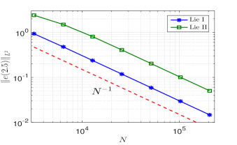
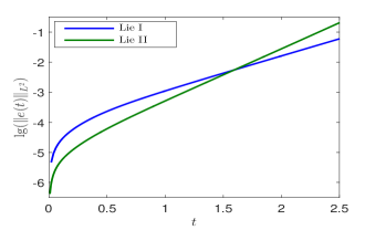
Figure 1. Temporal errors of the Lie-Trotter splitting (3.8) and (3.10) for the solitary wave (6.1).

Fig. 1 displays the temporal errors of the Lie-Trotter splitting method (3.8) & (3.10) for the solitary wave. The left plot displays the errors at $t_{N}=T=2.5$ under different values of $N$. It can be clearly seen that via both cases of temporal grid, the Lie-Trotter splitting method converges at the first order in time. The right plot shows the evolution of the error when the step number $N$ is fixed as $N=25000$. We observe that the error increases exponentially in time for both cases and the error of Lie I increases a bit slower than that of Lie II, which suggests to choose Lie I for long time simulation.

Fig. 2 shows the error $\|e(2.5)\|_{L^{2}}$ for the methods Strang I and Strang II. It can be clearly observed that the splitting scheme converges at the second order in time and the error of Strang I is far less than that of Strang II. Moreover, for the method Strang II, it leads to a correct solution and is convergent quadratically only when the step number $N$ is large enough $N\geqslant N_{T}$. Fig. 3 depicts the evolution of the error obtained via Strang I and Strang II with fixed step number $N=25000$. We are surprised to find that the error of Strang I method increases linearly with respect to time while the error of Strang II increases exponentially in time by noticing that the longitudinal axis represents the error (left plot in Fig. 3) and the logarithm of error (right plot in Fig. 3), respectively. The excellent convergence behavior of Strang I is different from that of Lie I and we can benefit a lot in practical computation, especially for long time simulation. We postpone the analytical study of this method to a future work.

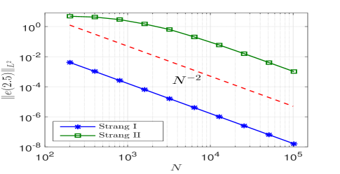
Figure 2. Temporal errors of the Strang splitting scheme (3.9)-(3.10) for the solitary wave solution (6.1) under different step numbers.

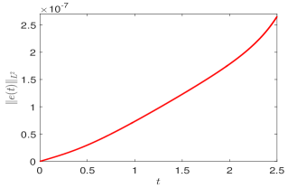
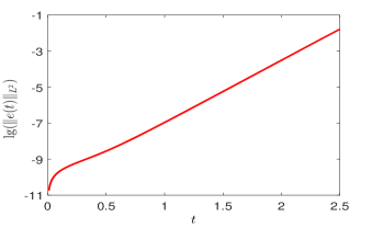
Figure 3. Error evolution by using Strang I (left) and Strang II (right) for the solitary wave (6.1).

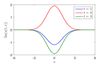
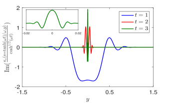
Figure 4. Dynamics of $u(t,x)$ (left) and $\kappa(s,y)$ (right) for the solitary wave (6.1).

For the solitary wave, it is easily checked that direct classical methods for $u$ work well since dispersion does not occur. On the contrary, the transform (3.1) (and (3.2)) makes the “essential” support of the solution $v$ (and $\kappa$) shrink exponentially with respect to time, as is shown in Fig. 4. This requires that the mesh size $h$ has to be set tinier and tinier as time evolves in order to capture the correct solution, which introduces huge costs if one keeps the computational domain fixed. However, this difficulty can be overcome by shrinking the computational region correspondingly in time, which enables the computational cost to be comparable with the direct splitting methods for (1.3) (regularized version).

This suggests that a reasonable way to proceed may be to first simulate (1.3) directly: if the solution is not dispersive, then nothing specific is needed (apart from the regularization of the logarithm). If the solution is dispersive (which is always the case when $\lambda>0$), then boundary effects become strong, and it is more efficient to consider (3.4) and use Strang I method via (3.9)–(3.10) on a nonuniform grid $\{s_{n}=\frac{\tanh(\omega t_{n})}{\omega}\}$.

Example 2. We set $\lambda=-3$ and $\omega=2$ in the equation (1.3). We consider the following several cases:
(i). $u_{0}(x)=2e^{-\alpha x^{2}/2}$ for $\alpha=2$;
(ii). $u_{0}(x)=2e^{-\alpha x^{2}/2}$ for $\alpha=1/2$;
(iii). $u_{0}(x)=\mathrm{sech}(x^{2}/2)$.

According to Proposition 2.1, for $\lambda=-3$, $\omega=2$, there exist two stationary solutions. The ODE (2.4)

$$\ddot{\mu}=\left(\frac{1}{\mu^{2}}-k_{-}\right)\left(\frac{1}{\mu^{2}}-k_{+}\right)\mu,\quad k_{\pm}=-\lambda\pm\sqrt{\lambda^{2}-\omega^{2}},$$

produces different trajectories due to different initial data for $\mu$, which is illustrated in Fig. 5 displaying the phase portrait for the equation (2.4).

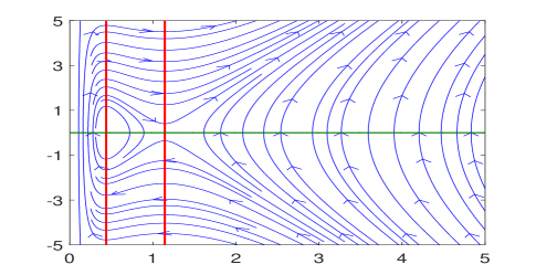
Figure 5. Phase portraits for the ODE (2.4) with $\omega=2$ and $\lambda=-3$.

For Case (i), $\alpha=2$ corresponds to $\mu(0)=1/\sqrt{\alpha}=1/\sqrt{2}$, $\dot{\mu}(0)=0$, which lies in the region producing time periodic solution $\mu(t)$, as seen from Fig. 5. This is confirmed by the dynamics shown in Fig. 6. We remark here that Fig. 6 is obtained by the standard Strang splitting method for (1.3) directly to avoid necessary treatments including adaptive mesh refinement and computational domain cut, since there is no dispersion for $u$.

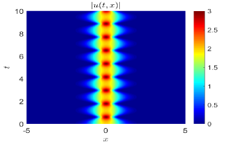
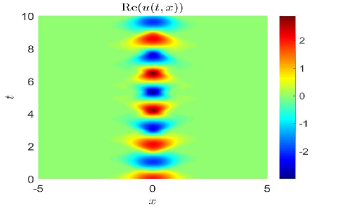
Figure 6. Dynamics of $u$ for Case (i) initial data in Example 2.

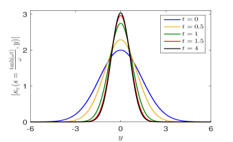
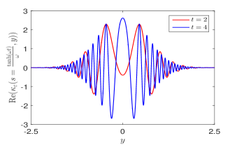
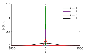
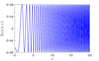
Figure 7. Dynamics of $\kappa$ (top) and $u$ (bottom) for Case (ii) initial data in Example 2.

Fig. 7 shows the dynamics of $\kappa_{\varepsilon}(s,y)$ for Case (ii) initial data by using Strang I method till $T=4$, or equivalently $s=\tanh(4\omega)/\omega$ with time step $\tau=0.0001$ and mesh size $h=1/2^{10}$. It can be observed that $\kappa_{\varepsilon}$, or accordingly $\kappa$, is well localized in space and $|\kappa(s,y)|$ stays almost invariant after some time (cf. the top left one in Fig. 7), however, the argument of $\kappa$ varies in time (the top right one in Fig. 7). Moreover, $\kappa$ oscillates in space. The bottom part in Fig. 7 shows the profile of $u(t,x)$ obtained by (3.10), which shows the dispersion of $u$. The right one displays $\operatorname{Re}(u(4,x))$, which shows that $u$ is highly oscillatory in space. The oscillation is more and more drastic when observed further away from the origin, which agrees with the transformation (3.10), due to the term $\exp\left(i\frac{\omega}{2}x^{2}\tanh(\omega t_{n})\right)$. Because of the rapid expansion and drastic oscillation in space, it is a disaster if one solves (1.3) directly.

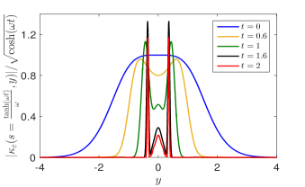
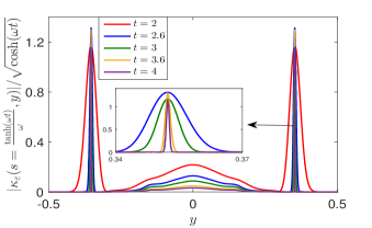
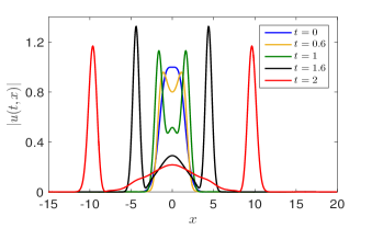
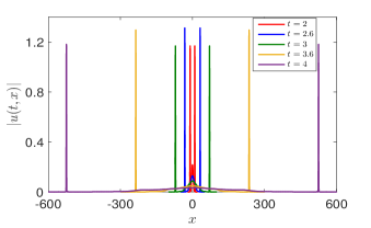
Figure 8. Dynamics of $\kappa(s,y)$ (top) and $u(t,x)$ (bottom) for Case (iii) in Example 2.

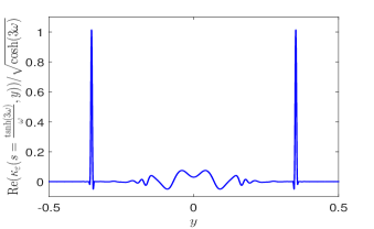
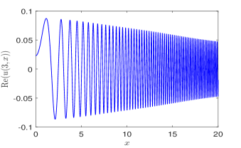
Figure 9. The profile of ($\operatorname{Re}\kappa_{\varepsilon}(s=\frac{\tanh(3\omega)}{\omega},y)$) (left) and $\operatorname{Re}(u(3,x))$ (right) for Case (iii) in Example 2.

Fig. 8 shows the profile of $\kappa(s,y)$ for Case (iii) initial data. Different from Case (ii) where the modulus of $\kappa$ keeps invariant after some time, here the modulus keeps increasing with respect to time, which is illustrated in the top graphics. The wave is split into two symmetric wave packets and a wave in between. As time evolves, the width of the two wave packets gets narrower and narrower. With the formulation (3.10), we get the dynamics of $u(t,x)$ in the bottom in Fig. 8. We observe that the initial wave is split into two symmetric breathers which spread out quickly (exponentially) in space with modulus varying periodically in time and a dispersive wave in between. Fig. 9 displays the profile of $\operatorname{Re}(\kappa)$ and $\operatorname{Re}(u)$ at $t=3$, which suggests the feasibility of solving $u$ via the formulation (3.10) and the virtual difficulty of solving $u$ directly.

Example 3. We set $\lambda=-2$ and $\omega=2$ in the equation (1.3), in which case there exists a continuous family of solitary wave when $u_{0}(x)=Ae^{-\alpha x^{2}/2}$ for $\alpha=2$ (or, equivalently $\mu(0)=1/\sqrt{2}$), according to Proposition 2.1, that can be illustrated from the phase portrait for the ODE (2.4) (cf. Fig. 10). We consider the following three cases for the initial data $u_{0}$:
(i). $u_{0}(x)=2e^{-\alpha x^{2}/2}$ for $\alpha=3$;
(ii). $u_{0}(x)=2e^{-\alpha x^{2}/2}$ for $\alpha=1/2$;
(iii). $u_{0}(x)=\mathrm{sech}(x^{2}/2)$.

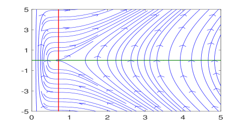
Figure 10. Phase portraits for the ODE (2.4) with $\omega=2$ and $\lambda=-2$.

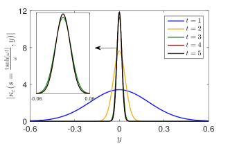
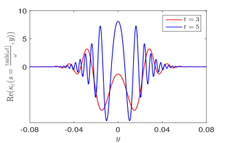
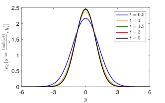
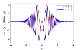
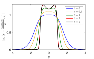
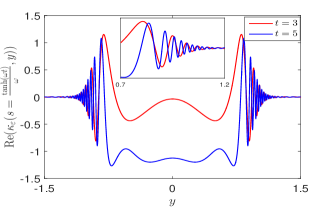
Figure 11. Dynamics of $\kappa$ for Cases (i)-(iii) (up to down) in Example 3.

Fig. 11 shows the dynamics of $\kappa$ until $s=\frac{\tanh(\omega T)}{\omega}$ for $T=5$ by using the method Strang I with $\tau=0.0002$ and $h=1/2^{12}$ on a computational domain $\Omega=(-10,10)$ with periodic boundary condition. We observe that for all three cases, the modulus $|\kappa|$ remain invariant after some time while the variation of the argument introduces the oscillation of $\kappa$ in space. This suggests that $|u|$ decreases exponentially in time, with rate $e^{-\omega t/2}$ in view of (3.10). Moreover, the argument of $\kappa$ introduces more and more oscillation in space as time involves (cf. the right column in Fig. 11).

Example 4. We set $\lambda=1$ and $\omega=2$ in the equation (1.3), in which case there exists no stationary solution for equation (2.4). We consider the following two cases for the initial data $u_{0}$:
(i). $u_{0}(x)=\mathrm{sech}(x^{2}/2)\sin(x)$;
(ii). $u_{0}(x)=2e^{-(x-3)^{2}/4}+2e^{-(x+3)^{2}}$.

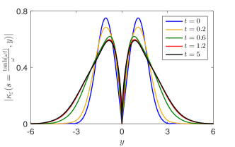
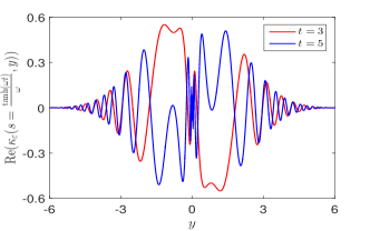
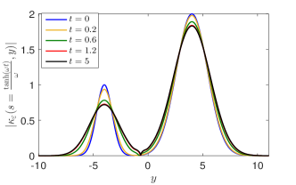
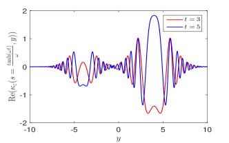
Figure 12. Dynamics of $\kappa$ for Cases (i)-(ii) (up to down) in Example 4.

Fig. 12 shows the dynamics of $\kappa$ until $s=\frac{\tanh(\omega T)}{\omega}$ for $T=5$ with $\tau=0.0002$ and $h=1/2^{12}$ on a computational domain $\Omega=(-20,20)$ with periodic boundary condition. We observe that the behavior is similar to that in Example 3, the modulus can attain the invariant state soon and more and more mild oscillations are created as time evolves. With the formulation (3.1), the dispersion and oscillation properties of $u$ can be clearly revealed.

Next we display some numerical experiments for dynamics of the solution $v$ for the equation (4.4), or accordingly the dynamics of $u$ (through (4.9)) for the power nonlinearity case (4.1). We still use Strang I method for temporal discretization with $\tau=0.0002$ and $h=1/2^{10}$ as the spatial mesh size on a computational domain $\Omega=(-20,20)$ with periodic boundary condition.

Example 5. We set $\lambda=1$, $\omega=2$ in the equation (4.1) with different $\sigma$ and initial data $u_{0}$:
(i). $u_{0}(x)=2e^{-x^{2}}$;
(ii). $u_{0}(x)=\mathrm{sech}(x^{2}/2)\sin(x)$.

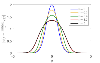
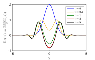
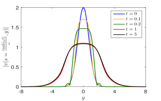
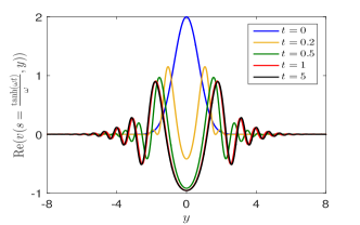
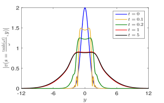
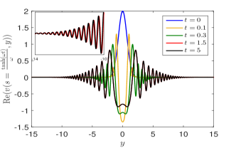
Figure 13. Dynamics of $v$ with $\sigma=1,2,3$ (up to down) for Case (i) initial data in Example 5.

Figs. 13 and 14 display the dynamics of $v$ for Cases (i) and (ii) initial data, respectively. We observe that for both cases and all chosen $\sigma=1,2,3$, both the modulus $|v|$ and the argument varies very slowly (almost invariant) after some time, which is different from the case with logarithmic nonlinearity where the argument varies quickly with respect to time. For Case (i) initial data, the “essential” support of the (almost) invariant state gets larger (cf. left column in Fig. 13) and more and more oscillation is created in space (cf. right column in Fig. 13) when $\sigma$ increases. While for Case (ii) initial data, one can hardly tell any remarkable difference for various choices of $\sigma$, as shown in Fig. 14.

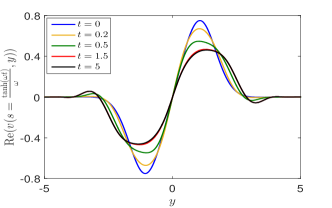
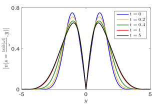
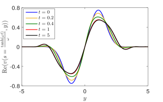
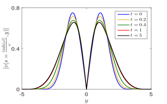
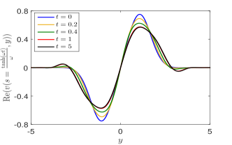
Figure 14. Dynamics of $v$ with $\sigma=1,2,3$ (up to down) for Case (ii) initial data in Example 5.

In the above examples, the numerical solution of (4.4) stays almost invariant after some time. This is understandable by noticing that the exponent in (4.6) gets very small as $t_{n}$ increases, and due to the rapid convergence toward the linear dynamics, recalled in (4.2), as well as the linear behavior, which involves, asymptotically as $t\to+\infty$, the same rescaling and phase shift as in (3.1).

Example 6. We set $\lambda=-1$, $\omega=2$ in the equation (4.1) with initial data $u_{0}(x)=2e^{-x^{2}}$ and different $\sigma$.

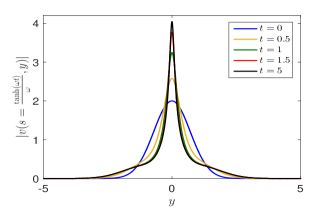
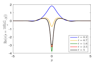
Figure 15. Dynamics of $v$ in the equation (4.5) with $\sigma=1$ in Example 6.

As was shown in [19], finite-time blow-up might occur when the parameters $\lambda$, $\omega$, $\sigma$ and $u_{0}$ satisfy some condition. Here we choose $\sigma=1,2,3$, respectively, and solve the equation (4.5) by Strang I method. For $\sigma=1$, the dynamics of $v$ is shown in Fig. 15. Similar results are obtained as in the case $\lambda>0$, which suggests that in this case, the solution in $u$ has the same dispersion as before, i.e., it disperses exponentially in time at the rate $e^{\omega t/2}$. While for $\sigma=3$, the dynamics of $v$ is displayed in Fig. 16, from which we observe that the solution concentrates around the origin quickly. This is in agreement with the virial computation leading to [19, Theorem 1.1, case 3]: in the present case we check that

$$\frac{1}{2}\|\nabla u_{0}\|_{L^{2}}^{2}+\frac{\lambda}{\sigma+1}\|u_{0}\|_{L^{2\sigma+2}}^{2\sigma+2}<-\frac{\omega^{2}}{2}\|xu_{0}\|_{L^{2}}^{2}-\omega\left|\operatorname{Im}\int\overline{u_{0}}x\cdot\nabla_{x}u_{0}\right|,$$

as every term can be computed in the Gaussian case, and so the solution blows up in the future and in the past. The right plot shows the dynamics of $\nabla v$, which suggests that blow-up (4.3) occurs at around $T=0.02445$. The situation is similar for $\sigma=2$, which is omitted here for brevity. In one word, the proposed method based on the formulation (3.1) is able to capture the correct dynamics for both dispersive solutions and finite-time blow-up solutions. It is superior than that by solving the original equation (4.1) directly when the finite-time blow-up does not occur so soon.

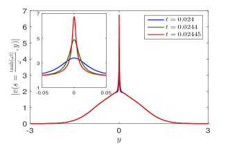
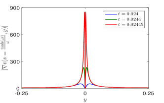
Figure 16. Dynamics of $v$ in the equation (4.5) with $\sigma=3$ in Example 6.

7. Conclusion

We proposed some time splitting methods for the Schrödinger equation with a logarithmic nonlinearity and a repulsive potential based on the generalized lens transform. This transformation can capture the main dispersion and oscillation in the solution. It neutralizes the possible boundary effects and enables the classical splitting methods to work smoothly for the equivalent formulation. This approach was extended to the case with a power nonlinearity. Error estimates for the semi-discrete Lie-Trotter splitting method were established for the equation with both types of nonlinearities. Finally we investigated the dynamics and revealed the dispersion property of the mentioned two types of equations with different parameters by employing the proposed methods.

References

- [1] E. R. Abraham, N. W. Ritchie, W. I. McAlexander, and R. G. Hulet, Photoassociative spectroscopy of long-range states of ultracold 6Li2 and 7Li2, J. Chem. Phys., 103 (1995), pp. 7773–7778.
- [2] X. Antoine, C. Besse, and P. Klein, Absorbing boundary conditions for the one-dimensional Schrödinger equation with an exterior repulsive potential, J. Comput. Phys., 228 (2009), pp. 312–335.
- [3] , Absorbing boundary conditions for the two-dimensional Schrödinger equation with an exterior potential part I: construction and a priori estimates, Math. Models Meth. Appl. Sci., 22 (2012), p. 1250026.
- [4] , Absorbing boundary conditions for the two-dimensional Schrödinger equation with an exterior potential, Numer. Math., 125 (2013), pp. 191–223.
- [5] A. H. Ardila, Orbital stability of Gausson solutions to logarithmic Schrödinger equations, Electron. J. Differential Equations, (2016), pp. Paper No. 335, 9.
- [6] A. H. Ardila, L. Cely, and M. Squassina, Logarithmic Bose-Einstein condensates with harmonic potential, Asymptotic Anal., 116 (2020), pp. 27–40.
- [7] A. V. Avdeenkov and K. G. Zloshchastiev, Quantum Bose liquids with logarithmic nonlinearity: Self-sustainability and emergence of spatial extent, J. Phys. B: Atomic, Molecular Optical Phys., 44 (2011), p. 195303.
- [8] W. Bao, R. Carles, C. Su, and Q. Tang, Error estimates of a regularized finite difference method for the logarithmic Schrödinger equation, SIAM J. Numer. Anal., 57 (2019), pp. 657–680.
- [9] , Regularized numerical methods for the logarithmic Schrödinger equation, Numer. Math., 143 (2019), pp. 461–487.
- [10] W. Bao, R. Carles, C. Su, and Q. Tang, Error estimates of local energy regularization for the logarithmic Schrödinger equation, Math. Models Meth. Appl. Sci., (to appear, 2022).
- [11] J. A. Barceló, A. Ruiz, and L. Vega, Some dispersive estimates for Schrödinger equations with repulsive potentials, J. Funct. Anal., 236 (2006), pp. 1–24.
- [12] C. Besse, B. Bidégaray, and S. Descombes, Order estimates in time of splitting methods for the nonlinear Schrödinger equation, SIAM J. Numer. Anal., 40 (2002), pp. 26–40.
- [13] I. Białynicki-Birula and J. Mycielski, Nonlinear wave mechanics, Ann. Physics, 100 (1976), pp. 62–93.
- [14] , Gaussons: Solitons of the logarithmic Schrödinger equation, Special issue on solitons in physics, Phys. Scripta, 20 (1979), pp. 539–544.
- [15] B. Bouharia, Stability of logarithmic Bose–Einstein condensate in harmonic trap, Mod. Phys. Lett. B, 29 (2015), p. 1450260.
- [16] H. Buljan, A. Šiber, M. Soljačić, T. Schwartz, M. Segev, and D. Christodoulides, Incoherent white light solitons in logarithmically saturable noninstantaneous nonlinear media, Phys. Rev. E, 68 (2003), p. 036607.
- [17] J. P. Burke Jr, C. H. Greene, and J. L. Bohn, Multichannel cold collisions: Simple dependences on energy and magnetic field, Phys. Rev. Lett., 81 (1998), p. 3355.
- [18] R. Carles, Critical nonlinear Schrödinger equations with and without harmonic potential, Math. Models Methods Appl. Sci., 12 (2002), pp. 1513–1523.
- [19] , Nonlinear Schrödinger equations with repulsive harmonic potential and applications, SIAM J. Math. Anal., 35 (2003), pp. 823–843.
- [20] R. Carles and G. Ferriere, Orbital stability of Gausson solutions to logarithmic Schrödinger equations, Nonlinearity, 34 (2021), pp. 8283–8310.
- [21] R. Carles and I. Gallagher, Universal dynamics for the defocusing logarithmic Schrödinger equation, Duke Math. J., 167 (2018), pp. 1761–1801.
- [22] R. Carles and L. Gosse, Numerical aspects of nonlinear Schrödinger equations in the presence of caustics, Math. Models Methods Appl. Sci., 17 (2007), pp. 1531–1553.
- [23] R. Carles and C. Su, Nonuniqueness and nonlinear instability of Gaussons under repulsive harmonic potential, arXiv:2107.10024, (2021).
- [24] , Scattering and uniform in time error estimates for splitting method in NLS. Preprint, archived at https://hal.archives-ouvertes.fr/hal-03403443, 2021.
- [25] T. Cazenave, Stable solutions of the logarithmic Schrödinger equation, Nonlinear Anal., 7 (1983), pp. 1127–1140.
- [26] T. Cazenave, Semilinear Schrödinger equations, vol. 10 of Courant Lecture Notes in Mathematics, New York University Courant Institute of Mathematical Sciences, New York, 2003.
- [27] W. Choi and Y. Koh, On the splitting method for the nonlinear Schrödinger equation with initial data in , Discrete Contin. Dyn. Syst., 41 (2021), pp. 3837–3867.
- [28] A. Gallagher and D. E. Pritchard, Exoergic collisions of cold Na∗-Na, Phys. Rev. Lett., 63 (1989), p. 957.
- [29] B. Gao, Repulsive interaction, Phys. Rev. A, 59 (1999), p. 2778.
- [30] L. Greengard and J.-Y. Lee, Accelerating the nonuniform fast Fourier transform, SIAM Review, 46 (2004), pp. 443–454.
- [31] T. Hansson, D. Anderson, and M. Lisak, Propagation of partially coherent solitons in saturable logarithmic media: A comparative analysis, Phys. Rev. A, 80 (2009), p. 033819.
- [32] E. F. Hefter, Application of the nonlinear Schrödinger equation with a logarithmic inhomogeneous term to nuclear physics, Phys. Rev. A, 32 (1985), pp. 1201–1204.
- [33] L. I. Ignat, A splitting method for the nonlinear Schrödinger equation, J. Differ. Equations, 250 (2011), pp. 3022–3046.
- [34] L. I. Ignat and E. Zuazua, Dispersive properties of numerical schemes for nonlinear Schrödinger equations, in Foundations of computational mathematics, Santander 2005. Selected papers based on the presentations at the international conference of the Foundations of Computational Mathematics (FoCM), Santander, Spain, June 30 – July 9, 2005., Cambridge: Cambridge University Press, 2006, pp. 181–207.
- [35] , Numerical dispersive schemes for the nonlinear Schrödinger equation, SIAM J. Numer. Anal., 47 (2009), pp. 1366–1390.
- [36] S. Jiang, L. Greengard, and W. Bao, Fast and accurate evaluation of nonlocal Coulomb and dipole-dipole interactions via the nonuniform FFT, SIAM J. Sci. Comput., 36 (2014), pp. B777–B794.
- [37] W. Krolikowski, D. Edmundson, and O. Bang, Unified model for partially coherent solitons in logarithmically nonlinear media, Phys. Rev. E, 61 (2000), pp. 3122–3126.
- [38] E. Lorin, S. Chelkowski, and A. Bandrauk, A numerical Maxwell–Schrödinger model for intense laser–matter interaction and propagation, Comput. Phys. Commun., 177 (2007), pp. 908–932.
- [39] C. Lubich, On splitting methods for Schrödinger-Poisson and cubic nonlinear Schrödinger equations, Math. Comp., 77 (2008), pp. 2141–2153.
- [40] S. D. Martino, M. Falanga, C. Godano, and G. Lauro, Logarithmic Schrödinger-like equation as a model for magma transport, Europhys. Lett., 63 (2003), pp. 472–475.
- [41] J. Miller, R. Cline, and D. Heinzen, Photoassociation spectrum of ultracold Rb atoms, Phys. Rev. Lett., 71 (1993), p. 2204.
- [42] R. Napolitano, J. Weiner, C. J. Williams, and P. S. Julienne, Line shapes of high resolution photoassociation spectra of optically cooled atoms, Phys. Rev. Lett., 73 (1994), p. 1352.
- [43] U. Niederer, The maximal kinematical invariance groups of the harmonic oscillator, Helv. Phys. Acta, 46 (1973), pp. 191–200.
- [44] C. Orzel, S. Bergeson, S. a. Kulin, and S. Rolston, Time-resolved studies of ultracold ionizing collisions, Phys. Rev. Lett., 80 (1998), p. 5093.
- [45] P. Paraschis and G. E. Zouraris, On the convergence of the Crank-Nicolson method for the logarithmic Schrödinger equation. Submitted, 2021.
- [46] M. Reed and B. Simon, Methods of modern mathematical physics. IV Analysis of Operators, Academic Press, New York, 1978.
- [47] W. C. Stwalley, Simple long-range model and scaling relations for the binding of isotopic hydrogen atoms to isotopic helium surfaces, Chem. Phys. Lett., 88 (1982), pp. 404–408.
- [48] C. Zhang and X. Zhang, Bound states for logarithmic Schrödinger equations with potentials unbounded below, Calc. Var. Partial Differential Equations, 59 (2020), pp. Paper No. 23, 31.
- [49] K. G. Zloshchastiev, Logarithmic nonlinearity in theories of quantum gravity: Origin of time and observational consequences, Grav. Cosmol., 16 (2010), pp. 288–297.
- [50] K. G. Zloshchastiev, Spontaneous symmetry breaking and mass generation as built-in phenomena in logarithmic nonlinear quantum theory, Acta Phys. Pol. B, 42 (2010), pp. 261–292.