All-order correlation of single excitons in nanocrystals using a
$\mathbf{k}\cdot\mathbf{p}$ envelope-function approach: application to lead-halide perovskites

Abstract

We discuss a variety of many-body approaches, within effective-mass and $\mathbf{k}\cdot\mathbf{p}$ envelope-function formalisms, for calculating correlated single excitons in semiconductor nanocrystals (NCs) to all orders in the electron-hole Coulomb interaction. These approaches are applied to NCs of the lead-halide perovskite CsPbBr₃, which typically present excitons in intermediate confinement with physical observables often strongly renormalized by correlation (e.g., radiative decay rate enhanced by a factor of about 7 relative to a mean-field approach, for a NC of edge length 11 nm). The many-body methods considered include the particle-hole Bethe-Salpeter equation, configuration interaction with single excitations, and the random-phase approximation with exchange (RPAE), which are shown to be closely related to each other but to treat $\mathbf{k}\cdot\mathbf{p}$ corrections differently, with RPAE being the most complete method. The methods are applied to calculate the correlation energy, the radiative lifetime, and the long-range Coulomb contribution to the fine structure of the ground-state exciton. In the limit of large NC sizes, the numerical results are shown to agree well with analytical results for this limit, where these are known. Correlated excited states of the single exciton are used to calculate the one-photon absorption cross section; the shape of the resulting cross-section curve (versus laser wavelength) at threshold and up to an excitation energy of about 1 eV is in good agreement with experimental cross sections. The equations for the methods are explicitly adapted to spherical symmetry (involving radial integrals and angular factors) and in this form permit a rapid computation for systems in intermediate confinement.

I Introduction

In 2015, Protesescu et al. [1] reported a new class of semiconductor nanocrystal (NC) materials, all-inorganic lead-halide perovskites CsPbX₃ (X = Cl, Br, I), having exceptional optoelectronic properties. These NCs emit and absorb strongly, are free from blinking, and the emission frequency can be tuned over the whole visible range by varying the NC size and the halide composition X (including mixtures of different halides) [1, 2]. This has led to numerous recent applications [3] to light-emitting diodes [4, 5], lasers [6, 7], and single-photon sources [8], among others.

The typical size range of the synthesized NCs is 6–16 nm [1, 9, 10, 2], which is comparable to or greater than the semiconductor Bohr diameter ($2a_{B}\approx 6$ nm for CsPbBr₃; see Sec. III.1). Consequently, excitons in these NCs are in the regime of intermediate confinement, with partially formed bound excitons having a strong correlation between electron and hole. This correlation can have important consequences. For instance, the radiative decay rate of the band-edge exciton in CsPbBr₃ is enhanced [11, 12] by factors of order 3–16 (depending on NC size in the range 6–16 nm) compared to its value calculated assuming noninteracting carriers [2] or a mean-field treatment of the carrier-carrier Coulomb interaction [13]. In general, special many-body techniques are necessary to treat intermediate confinement theoretically.

In this paper, we revisit the question of correlated single excitons in the context of inorganic lead-halide perovskite NCs. A commonly used approach to compute exciton properties in NCs is configuration interaction (CI) [12, 14, 15, 16]. Quantum Monte Carlo has also been used [15]. Recent applications to NCs of CsPbX₃ have involved Hartree-Fock (HF) and low orders of many-body perturbation theory (MBPT) [17, 13], and a one-parameter variational method [2, 18, 19] introduced by Takagahara [12].

We employ an envelope-function approach [20] and consider both the effective-mass approximation (EMA) and $\mathbf{k}\cdot\mathbf{p}$ models in which the valence band (VB) and conduction band (CB) are coupled, such as the $4\times 4$ and $8\times 8$ $\mathbf{k}\cdot\mathbf{p}$ models [21]. The latter enable one to compute the “$\mathbf{k}\cdot\mathbf{p}$ corrections” to the EMA, which account for nonparabolic terms in the band dispersion as well as VB-CB mixing induced by the finite size of the NC [22]. We consider approaches to correlation in which the carrier-carrier Coulomb interaction is treated to all orders of perturbation theory. We start from a CI expansion, a basic all-order approach, and then generalize this to include a more complete treatment of $\mathbf{k}\cdot\mathbf{p}$ corrections. An important aspect of our formalism is that the equations are adapted explicitly to spherical symmetry, involving 1D radial integrals and angular factors, which leads to a computationally efficient procedure in intermediate confinement. Applications are given to NCs of CsPbBr₃ and compared with recent experiments.

The paper is organized as follows. In Sec. II, we discuss the all-order many-body formalisms that we employ. The spherical reduction of the many-body equations to radial integrals and angular factors is given in the Appendix. The applications to CsPbBr₃ are then described in Sec. III. First, in Sec. III.1, we give the material parameters for bulk CsPbBr₃ needed as input to the EMA and $\mathbf{k}\cdot\mathbf{p}$ models. Some of these parameters remain rather uncertain at present. We also discuss the “quasi-cubic” spherical confining potential used to model the cuboid NCs of CsPbBr₃. Applications are then given to the correlation energy (Sec. III.2), the ground-state radiative lifetime (Sec. III.3), the long-range Coulomb contribution to the exciton fine structure (Sec. III.4), and the one-photon absorption cross section (Sec. III.5). In Secs. III.2–III.4 we also discuss the analytical results that can be derived for the EMA in two cases: noninteracting carriers and in the limit of large NC sizes. Partly as a test of our methods, we check where possible that in the large-size limit our numerical procedures give the expected results.

Our conclusions are given in Sec. IV. Throughout, all formulas are given in atomic units (a.u.), $\hbar=|e|=m_{0}=4\pi\epsilon_{0}=1$.

II All-order correlated excitons

We consider a set of interacting carriers (electrons and holes) confined by a mesoscopic potential $V_{\text{ext}}(\mathbf{r})$. The bulk band structure is described by a $\mathbf{k}\cdot\mathbf{p}$ Hamiltonian $h_{\mathbf{k}\cdot\mathbf{p}}$ and carrier states are expressed in terms of products of envelope and Bloch functions [20]. The total Hamiltonian is

$$H=\sum_{ij}\{i^{\dagger}j\}\langle i|h_{\mathbf{k}\cdot\mathbf{p}}+V_{\text{ext}}|j\rangle+\frac{1}{2}\sum_{ijkl}\{i^{\dagger}j^{\dagger}lk\}\langle ij|g_{12}|kl\rangle\,,$$ (1)

where $i,j,\ldots$, etc., refer to the electron states in the bands (valence and conduction) included in the calculation, and the notation $\{i_{1}^{\dagger}i_{2}^{\dagger}\ldots j_{1}j_{2}\ldots\}$ indicates a normally ordered product of creation (and annihilation) operators for electron states $i_{1},i_{2},\ldots$ (and $j,j_{2},\ldots$ ). The Hamiltonian $h_{\mathbf{k}\cdot\mathbf{p}}$ can can include a $\mathbf{k}\cdot\mathbf{p}$ coupling term between the VB and the CB, as in the $8\times 8$ or $4\times 4$ $\mathbf{k}\cdot\mathbf{p}$ models [21]. Alternatively, the VB and CB can be uncoupled, as in EMA models [20]. We consider both cases in the following.

In envelope-function formalisms, the Coulomb interaction is a sum of long-range (LR) and short-range (SR) terms [23],

$$g_{12}=g_{12}^{\text{LR}}+g_{12}^{\text{SR}}\,.$$ (2)

The LR term has the form of the usual Coulomb interaction

$$g_{12}^{\text{LR}}=\frac{1}{\varepsilon_{\text{in}}|\mathbf{r}_{1}-\mathbf{r}_{2}|}\,,$$ (3)

including a suitable dielectric constant $\varepsilon_{\text{in}}$ for the semiconductor material (which should correspond to low frequencies and a length scale of the size of the NC). We will not do so in the applications here, but the LR Coulomb interaction can also be generalized using macroscopic electrostatics [24] to a system of dielectrics, where induced polarization charges form near the boundaries between different materials—for example, in studies of the effect of the dielectric mismatch with the environment [25].

The SR term is a contact interaction [23],

$$g_{12}^{\text{SR}}=\gamma^{\text{SR}}\delta^{3}(\mathbf{r}_{1}-\mathbf{r}_{2})\,.$$ (4)

In discussions of exciton fine structure, the constant $\gamma^{\text{SR}}$ is proportional to the exchange Coulomb matrix element between the Bloch states of the VB and CB [23, [][[Sov.Phys.JETP33, 108(1971)].]pikus-71-sqd]. The SR term $g_{12}^{\text{SR}}$ is formally of order $(L_{\text{atom}}/L_{\text{meso}})^{2}$ [23], where $L_{\text{meso}}$ the mesoscopic length scale (the size of the quantum dot or the semiconductor Bohr radius) and $L_{\text{atom}}$ is the atomistic length scale. In a finite-size system, the quantity $L_{\text{atom}}/L_{\text{meso}}$ is also the small parameter that appears in $\mathbf{k}\cdot\mathbf{p}$ perturbation theory, $\mathbf{k}\cdot\mathbf{p}\sim L_{\text{atom}}/L_{\text{meso}}$, and the SR Coulomb interaction thus has a leading order $O[(\mathbf{k}\cdot\mathbf{p})^{2}]$. By contrast, the LR Coulomb interaction typically gives larger contributions of order $O(1)$ in $\mathbf{k}\cdot\mathbf{p}$ perturbation theory, with the $\mathbf{k}\cdot\mathbf{p}$ terms providing small corrections (see below). An exception can occur when the leading orders of the LR Coulomb term are suppressed for some reason. This happens in the exciton fine structure, where the leading LR Coulomb term is also $O[(\mathbf{k}\cdot\mathbf{p})^{2}]$ and the LR and SR terms thus yield contributions with a similar order of magnitude (see below and Sec. III.4). We will consider only the LR term in our applications, $g_{12}=g_{12}^{\text{LR}}$, although the general many-body formalism applies to the SR term as well.

We choose a single-particle basis $|i\rangle$ for the calculations satisfying

$$(h_{\mathbf{k}\cdot\mathbf{p}}+V_{\text{ext}}+U)|i\rangle=\epsilon_{i}|i\rangle\,,$$ (5)

where $U$ is a mean field, which is in principle arbitrary. Possible choices are an independent-particle basis $U=0$, or a HF basis $U=V_{\text{HF}}$, such as a configuration-averaged HF basis [17, 13], which takes account of the electron-hole ($e$-$h$) interaction in a mean-field approximation. We will take $V_{\text{ext}}$ and $U$ to be spherically symmetric. This will lead to computationally efficient procedures in which only the radial dimension needs to be treated numerically, while the angular dimensions can be handled analytically. Even though NCs of inorganic perovskites are cuboid [1], they can be well approximated for many purposes (e.g., ground-state energies, exciton fine structure, absorption cross sections) by a spherical “quasi-cubic” potential [27, 17, 13, 28]. Nonspherical terms in $V_{\text{ext}}$, arising from shape corrections to the NC or from the underlying crystal lattice, can in principle be treated later in the calculation as perturbations.

Noninteracting or mean-field states are physically appropriate only in the strong-confinement limit of small NC sizes $R$, where the carrier-carrier Coulomb energy is small compared to the kinetic energy and thus yields only a small perturbation of the independent-particle picture. As the NC grows in size and eventually exceeds the semiconductor Bohr radius $R>a_{B}$, partially bound excitons begin to form and an exciton expressed in the basis (5) acquires strong correlation corrections [11, 12].

We are interested here in studying such a confined exciton to all orders in the Coulomb interaction $g_{12}$. As a first step, we consider CI in the space of all single-exciton states [12, 14, 15, 16]. In this approach, a general correlated exciton state $|\alpha\rangle$ is written

$$|\alpha\rangle=\sum_{eh}\mathcal{X}_{eh}^{\alpha}|\psi_{eh}\rangle\,,$$ (6)

where $|\psi_{eh}\rangle$ is an uncorrelated single-exciton state containing an electron $e$ and a hole $h$,

$$|\psi_{eh}\rangle=\{e^{\dagger}h\}|0\rangle\,,$$ (7)

with $|0\rangle$ the effective vacuum (no carriers present in the NC). The amplitudes $\mathcal{X}_{eh}^{\alpha}$ in Eq. (6) are found from the CI eigenvalue problem

$$\sum_{e^{\prime}h^{\prime}}\langle\psi_{eh}|H|\psi_{e^{\prime}h^{\prime}}\rangle\mathcal{X}_{e^{\prime}h^{\prime}}^{\alpha}=\omega_{\alpha}\mathcal{X}_{eh}^{\alpha}\,,$$ (8)

and are normalized according to

$$\sum_{eh}|\mathcal{X}_{eh}^{\alpha}|^{2}=1\,.$$ (9)

To determine the matrix of the Hamiltonian $H$ in Eq. (8), we add and subtract the mean field $U$ from Eq. (1),

$$H = \sum_{i}\{i^{\dagger}i\}\epsilon_{i}+\frac{1}{2}\sum_{ijkl}\{i^{\dagger}j^{\dagger}lk\}\langle ij|g_{12}|kl\rangle$$ (10)

$${}+\sum_{ij}\{i^{\dagger}j\}\langle i|(-U)|j\rangle\,,$$

from which it follows that

$$\langle\psi_{eh}|H|\psi_{e^{\prime}h^{\prime}}\rangle = (\epsilon_{e}-\epsilon_{h})\delta_{ee^{\prime}}\delta_{hh^{\prime}}$$ (11)

$${}+\langle e|(-U)|e^{\prime}\rangle\delta_{hh^{\prime}}-\langle h^{\prime}|(-U)|h\rangle\delta_{ee^{\prime}}$$

$${}-\langle eh^{\prime}|g_{12}|e^{\prime}h\rangle+\langle eh^{\prime}|g_{12}|he^{\prime}\rangle\,.$$

Many-body diagrams for $\sum_{e^{\prime}h^{\prime}}\langle\psi_{eh}|H|\psi_{e^{\prime}h^{\prime}}\rangle\mathcal{X}_{e^{\prime}h^{\prime}}^{\alpha}$ are shown in Figs. 1(a)–(e).

To solve the eigenvalue problem (8), we generate a basis set containing all basis states $|e\rangle$ and $|h\rangle$ up to a high energy cutoff and compute the matrix elements $\langle\psi_{eh}|H|\psi_{e^{\prime}h^{\prime}}\rangle$. It is then possible to extract the eigenvalues $\omega_{\alpha}$ and eigenvectors $\mathcal{X}_{eh}^{\alpha}$ for the correlated ground-state exciton, $\alpha=0$, together with as many excited exciton states $\alpha>0$ as are desired. We find that the exciton energies $\omega_{\alpha}$ are nearly independent of the choice of mean field $U=0$ or $U=V_{\text{HF}}$ (there is no difference, for practical purposes, between these two choices of $U$). The main role of a HF mean field $U=V_{\text{HF}}$ in this formalism is that fewer basis states $|e\rangle$ and $|h\rangle$ are required to obtain a given precision (basis-set truncation error), since the HF basis states already contain mean-field information about the $e$-$h$ interaction and are more physical. We will refer to this approach as CI singles (CIS).

Figure 1: Excitations present in the various approaches to correlated excitons. Diagrams (a)–(e) represent $\sum_{e^{\prime}h^{\prime}}\langle\psi_{eh}|H|\psi_{e^{\prime}h^{\prime}}\rangle\mathcal{X}_{e^{\prime}h^{\prime}}^{\alpha}$ and correspond (in order) to the five terms in Eq. (11) for the CIS method. The BSE approach is given by the four diagrams (a)–(d). The RPAE method includes diagrams (a)–(e) and additionally the diagrams (f) and (g), which represent $\sum_{e^{\prime}h^{\prime}}B_{eh,e^{\prime}h^{\prime}}\mathcal{Y}_{e^{\prime}h^{\prime}}^{\alpha}$ and correspond (in order) to the two terms in Eq. (15). Notation: dashed horizontal line, Coulomb interaction; thick horizontal line, all-order amplitude; horizontal line with cross, potential counter-term $-U$.

The matrix element of a one-body operator $M=\sum_{ij}\{i^{\dagger}j\}\langle i|M|j\rangle$ between a correlated exciton state $|\alpha\rangle$ and the NC ground state $|0\rangle$ in the CIS approach is

$$\langle\alpha|M|0\rangle=\sum_{eh}(\mathcal{X}_{eh}^{\alpha})^{*}\langle e|M|h\rangle\,.$$ (12)

For example, $M$ could be the momentum operator that enters in interband absorption and emission [20].

When $V_{\text{ext}}+U$ is spherically symmetric, the basis states $|e\rangle$ and $|h\rangle$ have exact total angular momentum quantum numbers $F_{e}$ and $F_{h}$, respectively, which couple to an exact total angular momentum $F_{\text{tot}}$ for an exciton state [22]. Parity is also an exact quantum number. In the Appendix, we give the reduction of Eqs. (8)–(12) to radial integrals and angular factors for the spherical case. The computational gain in making this reduction is not only that 1D radial integrals are much faster to evaluate than 3D integrals, but also that the sums over magnetic substates can be performed analytically, so that the effective sizes of the basis set and the matrix $\langle\psi_{eh}|H|\psi_{e^{\prime}h^{\prime}}\rangle$ are much smaller. In the presence of nonspherical terms, these angular-momentum quantum numbers are only approximate.

In envelope-function $\mathbf{k}\cdot\mathbf{p}$ approaches, when the electron band index changes at one vertex of a Coulomb interaction, the matrix element is suppressed, being formally of order $O(\mathbf{k}\cdot\mathbf{p})$ in $\mathbf{k}\cdot\mathbf{p}$ perturbation theory [20]. Small “$\mathbf{k}\cdot\mathbf{p}$ corrections” of this sort correspond to nonparabolic terms in the electron dispersion relation and to VB-CB mixing induced by the finite size of the confining potential $V_{\text{ext}}$ [22]. The $\mathbf{k}\cdot\mathbf{p}$ corrections to Coulomb matrix elements can be picked up straightforwardly in $\mathbf{k}\cdot\mathbf{p}$ approaches in which the VB and CB are coupled, such as the $8\times 8$ or $4\times 4$ $\mathbf{k}\cdot\mathbf{p}$ models [21], where they arise as cross terms between small and large components of the carrier wave functions in the expression for the matrix element [17, 13]. Referring to Fig. 1, we see that in diagram (e), which corresponds to the last term in Eq. (11), the band index necessarily changes (from the VB to the CB) at both vertices of the Coulomb interaction, so that this term is formally of order $O[(\mathbf{k}\cdot\mathbf{p})^{2}]$. Diagram (e) corresponds to the $e$-$h$ exchange interaction. In contrast, the direct $e$-$h$ Coulomb interaction in diagram (d) has no change of band index at either vertex (for states $e$ and $e^{\prime}$ in the same CB, and states $h$ and $h^{\prime}$ in the same VB) and the term is therefore formally of $O(1)$ in $\mathbf{k}\cdot\mathbf{p}$ perturbation theory. It follows that to a good approximation we can drop the last (exchange) term $\langle eh^{\prime}|g_{12}|he^{\prime}\rangle$ in Eq. (11) and take only the first four terms. We will refer to this simplified approach as the particle-hole Bethe-Salpeter equation or BSE approach.

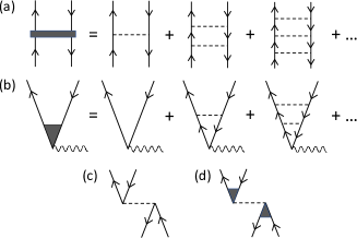
Figure 2: (a) Effective two-body interaction formed by summing all particle-hole ladder diagrams (arrows pointing up indicate electron states, arrows pointing down hole states); (b) all-order vertex correction to a one-body operator (e.g., momentum operator for interband absorption); (c) first-order Coulomb exchange interaction for exciton fine structure; (d) all-order Coulomb exchange interaction.

The relation to the particle-hole BSE can be seen by considering the perturbative (iterative) solution of the CI eigenvalue equation (8). The $O(1)$ diagram shown in Fig. 1(d), when iterated, generates an effective two-body interaction given by the sum of all particle-hole ladder diagrams [29], shown in Fig. 2(a). Use of the correlated final-state wave function $|\alpha\rangle$ to evaluate a matrix element of a one-body operator (12) will then bring in an all-order “vertex correction,” shown in Fig. 2(b), in which the Coulomb ladders connect the ingoing and outgoing states of the one-body operator. For NCs in intermediate confinement, the vertex correction can enhance the absorption rate by large factors [11, 12], for example, by as much as 3–16 for the ground-state exciton in NCs of the inorganic perovskite CsPbBr₃ [2, 13].

In the EMA, in which $\mathbf{k}\cdot\mathbf{p}$ corrections are absent, the BSE approach is entirely of order $O(1)$. In the following, we will denote this case BSE₀. It is also possible to use the BSE approach when the basis states are generated within a VB-CB-coupled $\mathbf{k}\cdot\mathbf{p}$ approximation, such as the $4\times 4$ or $8\times 8$ $\mathbf{k}\cdot\mathbf{p}$ models. This approach, which we denote BSE_k⋅p, brings in a subset of $\mathbf{k}\cdot\mathbf{p}$ corrections associated with the basis states. Clearly, further $\mathbf{k}\cdot\mathbf{p}$ corrections can be obtained by using the CIS approach instead, which includes additionally the $O[(\mathbf{k}\cdot\mathbf{p})^{2}]$ exchange diagram in Fig. 1(e). However, a still more complete treatment of $\mathbf{k}\cdot\mathbf{p}$ corrections is provided by an approach analogous to the random-phase approximation with exchange (RPAE) used in atomic and molecular physics [30] and cluster physics [31].

In RPAE, the CI eigenvalue problem (8) is replaced by a $2\times 2$ block eigenvalue problem [30]

$$\left(\begin{array}[]{cc}A&B\\ B^{*}&A^{*}\end{array}\right)\left(\begin{array}[]{c}\bm{\mathcal{X}}^{\alpha}\\ \bm{\mathcal{Y}}^{\alpha}\end{array}\right)=\omega_{\alpha}\left(\begin{array}[]{cc}1&0\\ 0&-1\end{array}\right)\left(\begin{array}[]{c}\bm{\mathcal{X}}^{\alpha}\\ \bm{\mathcal{Y}}^{\alpha}\end{array}\right)\,.$$ (13)

Here, $\bm{\mathcal{X}}^{\alpha}$ and $\bm{\mathcal{Y}}^{\alpha}$ are vectors of amplitudes $\mathcal{X}_{eh}^{\alpha}$ and $\mathcal{Y}_{eh}^{\alpha}$ in the space of uncorrelated excitons $(e,h)$, and the matrix $A$ is identical to that appearing in the CIS eigenvalue problem (8),

$$A_{eh,e^{\prime}h^{\prime}}=\langle\psi_{eh}|H|\psi_{e^{\prime}h^{\prime}}\rangle\,,$$ (14)

which is given in detail by Eq. (11). The matrix $B$ is

$$B_{eh,e^{\prime}h^{\prime}}=-\langle ee^{\prime}|g_{12}|h^{\prime}h\rangle+\langle ee^{\prime}|g_{12}|hh^{\prime}\rangle\,.$$ (15)

RPAE thus includes the dominant correlation diagrams of the BSE approach, Figs. 1(a)–(d), the additional exchange diagram of CIS, Fig. 1(e), and two further diagrams associated with the $B$ matrix, shown in Figs. 1(f) and (g). These two diagrams are both of order $O[(\mathbf{k}\cdot\mathbf{p})^{2}]$ in $\mathbf{k}\cdot\mathbf{p}$ perturbation theory. Physically, the $B$ matrix accounts for two-particle/two-hole correlations in the ground state [30]. The RPAE eigenvector is normalized according to

$$\sum_{eh}(|\mathcal{X}_{eh}^{\alpha}|^{2}-|\mathcal{Y}_{eh}^{\alpha}|^{2})=1\,,$$ (16)

and the matrix element (12) in RPAE becomes

$$\langle\alpha|M|0\rangle=\sum_{eh}[(\mathcal{X}_{eh}^{\alpha})^{*}\langle e|M|h\rangle+(\mathcal{Y}_{eh}^{\alpha})^{*}\langle h|M|e\rangle]\,.$$ (17)

The angular reduction of Eqs. (13)–(17) for a spherically symmetric potential is given in the Appendix.

Note that the many-body formalisms BSE, CIS, and RPAE, presented in Eqs. (6)–(17), apply to any single-particle basis $|i\rangle$ and not just to the envelope-function basis that we use in our applications. In Eq. (5), the term $h_{\mathbf{k}\cdot\mathbf{p}}+V_{\text{ext}}$ can be reinterpreted as any suitable effective single-particle Hamiltonian describing states of the finite-size NC.

III Application to perovskite nanocrystals

III.1 Parameters and model

Inorganic lead-halide perovskites are “inverted” direct-gap semiconductors having a $p_{1/2}$-like CB and an $s$-like VB. The VB maximum ($R_{6}^{+}$) and CB minimum ($R_{6}^{-}$) lie at the $R$ point of the Brillouin zone [1, 2]. This VB-CB pair can be described by the $4\times 4$ $\mathbf{k}\cdot\mathbf{p}$ model [32, 33, 2] or used for EMA calculations. The $p_{1/2}$-like CB is split by spin-orbit coupling from a higher-lying $p_{3/2}$-like band, whose minimum ($R_{8}^{-}$) lies about 1 eV above the minimum of the $p_{1/2}$-like band [2]. The $s$-like VB together with the $p_{1/2}$- and $p_{3/2}$-like CBs can be described by an extended $8\times 8$ $\mathbf{k}\cdot\mathbf{p}$ model [21].

The bulk CsPbBr₃ material parameters that we use are summarized in Table 1. The bandgap $E_{g}$ and reduced effective mass $\mu^{*}=m_{e}^{*}m_{h}^{*}/(m_{e}^{*}+m_{h}^{*})$ of the $s$-like VB and $p_{1/2}$-like CB were measured by Yang et al. [33] for the orthorhombic phase of CsPbBr₃ at cryogenic temperatures. While $\mu^{*}$ is known experimentally, the individual effective masses $m_{e}^{*}$ and $m_{h}^{*}$ are not. However, there is theoretical [2, 1] and experimental [34] evidence that $m_{e}^{*}$ and $m_{h}^{*}$ are approximately equal in inorganic lead-halide perovskites, so we will assume $m_{e}^{*}=m_{h}^{*}$. The spin-orbit coupling parameter $\Delta_{\text{soc}}$ is defined as the energy splitting of the $p_{3/2}$- and $p_{1/2}$-like CBs at the $R$ point; we estimate $\Delta_{\text{soc}}$ from a fit to the experimental absorption spectra (see Sec. III.5). Finally, the “effective” dielectric constant $\varepsilon_{\text{eff}}$ was inferred by Yang et al. [33] from the bulk exciton binding energy (see also Ref. [35]). Since $\varepsilon_{\text{eff}}$ applies to a length scale of order the semiconductor Bohr radius $a_{B}$, we use $\varepsilon_{\text{in}}=\varepsilon_{\text{eff}}$ to screen the carrier-carrier Coulomb interactions [Eq. (3)].

The Kane parameter $E_{P}$ has also not been measured. Estimates of $E_{P}$ were made in Ref. [17] based on the $4\times 4$ and $8\times 8$ $\mathbf{k}\cdot\mathbf{p}$ models discussed above, together with the assumption that remote bands (those not included in the model) make zero contribution. The resulting values $E_{P}^{(4\times 4)}$ and $E_{P}^{(8\times 8)}$ are given in Table 1 and can be seen to differ significantly. Given that the only difference between the two values is the inclusion of the $p_{3/2}$-like CB in $E_{P}^{(8\times 8)}$, it seems likely that other remote bands may make further significant contributions to $E_{P}$. An estimate using density-functional theory (DFT) [2] found $E_{P}=39.9$ eV, which seems quite high. As in Ref. [17], we take the view that $E_{P}$ is presently uncertain, a conservative range being $10\,\text{eV}\leq E_{P}\leq 40\,\text{eV}$. We will assume a value $E_{P}=20$ eV in our applications that is intermediate between $E_{P}^{(4\times 4)}$ and $E_{P}^{(8\times 8)}$.

Table 1: Bulk material parameters for CsPbBr₃ used in this paper. $E_{P}^{(4\times 4)}$ and $E_{P}^{(8\times 8)}$ are estimates of the Kane parameter derived in Ref. [17] from the $4\times 4$ and $8\times 8$ $\mathbf{k}\cdot\mathbf{p}$ models. The parameters $\varepsilon_{\text{eff}}$ and $\varepsilon_{\text{opt}}$ are the effective and optical dielectric constants of CsPbBr₃, respectively, and $\varepsilon_{\text{out}}$ is the optical dielectric constant of the surrounding medium. $\Delta_{\text{soc}}$ is the spin-orbit coupling parameter of the $8\times 8$ $\mathbf{k}\cdot\mathbf{p}$ model. Further explanation is given in Sec. III.1.

	CsPbBr3
$\mu^{*}$ ($\times m_{0}$)	$0.126$
$m_{e}^{*}=m_{h}^{*}$ ($\times m_{0}$)	$0.252$
$E_{g}$ (eV)	$2.342$
$E_{P}^{(4\times 4)}$ (eV)	$27.9$
$E_{P}^{(8\times 8)}$ (eV)	$16.4$
$E_{P}$ (eV)	$20.0$
$\Delta_{\text{soc}}$ (eV)	$0.8$
$\varepsilon_{\text{eff}}$	$7.3$
$\varepsilon_{\text{opt}}$	$4.84$
$\varepsilon_{\text{out}}$	$2.4$

NCs of CsPbBr₃ are cuboid [1]. For the above material parameters, one finds $2a_{B}=6.1$ nm, implying that NCs with edge lengths $L$ in the experimentally interesting range $L=6$–16 nm are in the regime of intermediate confinement, with strongly correlated excitons.

We take the confining potential to be a spherical well with infinite walls

$$V_{\text{ext}}^{\text{sph}}(r)=\left\{\begin{matrix}0\text{, if }r<R\\ \infty\text{, otherwise}\end{matrix}\right.\,.$$ (18)

The radius $R$ is chosen to be

$$R=L/\sqrt{3}\,,$$ (19)

which ensures that the noninteracting ground-state energy of a carrier (hole or electron) matches that in a cubic well with edge length $L$ [27, 17]. This quasi-cubic spherical potential can be shown to reproduce well other properties of a cubic well, such as the Coulomb energy of the $1S_{e}$-$1S_{h}$ exciton [17], the correlation energies of the trion and biexciton [17], and the one- [13] and two-photon [28] absorption cross sections.

III.2 Correlation energy of ground-state exciton

An example of a calculation of the correlation energy is given in Table 2. We here use the BSE₀ method (in the EMA) with a configuration-averaged HF basis set [17, 37] $U=V_{\text{HF}}$. The states of the basis set are cut off at principal quantum numbers $n_{\text{max}}=12$ in each angular-momentum channel ($s$, $p_{1/2}$, $p_{3/2}$, …, etc.). We then perform a series of calculations with the orbital angular momentum of the basis set truncated at $l_{\text{max}}=K$ for all $K$ in the range $1\leq K\leq 12$, giving a set of total exciton energies $E_{\text{tot}}(K)$. For $K\geq 2$, the partial-wave contribution $\delta E(K)$ for orbital angular momentum $K$ is defined as $\delta E(K)=E_{\text{tot}}(K)-E_{\text{tot}}(K-1)$. Since we define the correlation energy as the difference between the total energy and the configuration-averaged HF energy, $E_{\text{corr}}=E_{\text{tot}}-E_{\text{HF}}$, we can take the contribution for $K\leq 1$ to be $\delta E(K\leq 1)=E_{\text{tot}}(1)-E_{\text{HF}}$.

Table 2: Contribution $\delta E(K)$ of individual partial waves to the correlation energy of the ground-state $1S_{e}$-$1S_{h}$ exciton ($F_{\text{tot}}=1$), for NCs of CsPbBr₃ with edge lengths $L=9$ nm and 12 nm. Calculations are performed with the BSE₀ method using an EMA basis set. The correlation energy is here defined as the difference between the total exciton energy and the exciton energy in the configuration-averaged HF approximation (see Ref. [17] for more details), $E_{\text{corr}}=E_{\text{tot}}-E_{\text{HF}}$. We find $E_{\text{HF}}=0.08756199$ Ha for $L=9$ nm and $E_{\text{HF}}=0.08640365$ Ha for $L=12$ nm. Notation: $K$ is the partial wave (see text); ‘extrap.’ is the extrapolated sum of terms for $K=13$ to infinity. Units: mHa.

$K$	$L=9$ nm	$L=12$ nm
$\leq 1$	$-0.02624$	$-0.02782$
2	$-0.21087$	$-0.21166$
3	$-0.06176$	$-0.07328$
4	$-0.02343$	$-0.03096$
5	$-0.01053$	$-0.01491$
6	$-0.00534$	$-0.00792$
7	$-0.00297$	$-0.00455$
8	$-0.00177$	$-0.00277$
9	$-0.00112$	$-0.00178$
10	$-0.00074$	$-0.00119$
11	$-0.00050$	$-0.00082$
12	$-0.00036$	$-0.00058$
extrap.	$-0.00123$	$-0.00206$
Total	$-0.34683(1)$	$-0.38030(1)$

From Table 2, one sees that the correlation energy of the ground-state exciton $1S_{e}$-$1S_{h}$ is dominated by the contribution $K=2$, but higher partial waves also make significant contributions. Asymptotically for large $K$, one finds $\delta E(K)\sim 1/K^{3}$, which enables us to make an estimate of the contribution from $K=13$ to infinity. The estimated numerical error from the principal-quantum-number cutoff and partial-wave extrapolation is given in the final line. Note that, at the level of approximation used here (EMA and BSE₀), the two possible total angular momenta $F_{\text{tot}}=0$ and 1 of the ground-state $1S_{e}$-$1S_{h}$ exciton should be degenerate. However, it turns out that the partial-wave contributions for $F_{\text{tot}}=0$ and 1 are slightly different (e.g., for an edge length $L=9$ nm, $\delta E(2)=-0.21087$ mHa for $F_{\text{tot}}=1$ and $\delta E(2)=-0.17266$ mHa for $F_{\text{tot}}=0$). Nevertheless, we find that the final extrapolated energy for the two different values of $F_{\text{tot}}$ agree to within the estimated error shown in the table (which applies to $F_{\text{tot}}=1$), thus providing a useful test of the numerics.

A feature of this approach is that the partial-wave expansion becomes more slowly convergent as the NC size $L$ increases. This can be seen in Table 2, where the relative contribution to the correlation energy from the extrapolated terms $K\geq 13$ is greater for $L=12$ nm than for $L=9$ nm. In fact, the method eventually becomes unwieldy for edge lengths $L\gtrsim 50$ nm owing to the slow convergence, but for intermediate confinement in the experimentally interesting size range $6\,\text{nm}\leq L\leq 16\,\text{nm}$, one can readily achieve energies converged to a fractional error of 10^-3 or better in a few seconds of calculation on a single core.

Figure 3 shows the ground-state confinement energy in various many-body approximations (but all using the EMA), as a function of the NC edge length for $L=8$–30 nm. The confinement energy here is defined as

$$E_{\text{conf}}=E_{\text{tot}}-E_{g}\,.$$ (20)

Two cases can be handled analytically in the EMA. First, for noninteracting carriers, the ground-state single-particle wave function is

$$\psi_{1S}(\mathbf{r})=(2\pi R)^{-1/2}\frac{1}{r}\sin\left(\frac{\pi r}{R}\right)\,,$$ (21)

and the noninteracting confinement energy of a $1S_{e}$-$1S_{h}$ exciton is

$$E_{\text{non}}=\frac{\pi^{2}}{2\mu R^{2}}\,,$$ (22)

which tends to zero in the bulk limit $R\rightarrow\infty$.

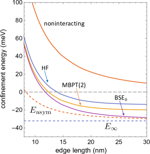
Figure 3: Ground-state exciton confinement energy [Eq. (20)] for a NC of CsPbBr₃ vs. NC edge length, in various approximations. All approaches assume the EMA. Continuous lines (top to bottom): ‘noninteracting’, noninteracting carriers; HF, configuration-averaged Hartree-Fock (following Ref. [17]); MBPT(2), many-body perturbation theory up to second order (following Ref. [17]); BSE₀, particle-hole Bethe-Salpeter equation. Dashed lines (top to bottom): $E_{\text{asym}}$, the large-$R$ asymptotic form of the confinement energy, Eq. (25); $E_{\infty}$, the $R\rightarrow\infty$ limit of the confinement energy, Eq. (26).

The bulk limit for interacting particles can also be handled analytically in the EMA, by solving a two-body Schrödinger equation [29],

$$\left(-\frac{1}{2m_{e}^{*}}\nabla_{e}^{2}-\frac{1}{2m_{h}^{*}}\nabla_{h}^{2}+\frac{1}{\varepsilon_{\text{in}}|\mathbf{r}_{e}-\mathbf{r}_{h}|}\right)\Psi(\mathbf{r}_{e},\mathbf{r}_{h})$$

$$\quad\quad\quad\quad\quad\quad\quad\quad\quad=\left(E_{\text{tot}}-E_{g}\right)\Psi(\mathbf{r}_{e},\mathbf{r}_{h})\,,$$ (23)

where $\Psi(\mathbf{r}_{e},\mathbf{r}_{h})$ goes to zero at the NC boundary. In Eq. (23), the electron and hole are effectively regarded as different species of particle, with one particle of each type present. It follows that a CI solution of Eq. (23) is formally identical to the method we called BSE₀ in Sec. II. In particular, since the electron and hole are regarded as distinguishable, the wave function $\Psi(\mathbf{r}_{e},\mathbf{r}_{h})$ is not required to be antisymmetric under interchange of electron and hole coordinates, and so the final exchange term in Eq. (11) is absent, as in the definition of the BSE₀ method. Also, as mentioned above, the spin-independence of the Hamiltonian has the consequence that the solutions for $F_{\text{tot}}=0$ and 1 are degenerate.

In the large-$R$ limit, Eq. (23) can be solved using relative $\mathbf{r}=\mathbf{r}_{e}-\mathbf{r}_{h}$ and center-of-mass (CM) $\mathbf{R}_{\text{CM}}=(m_{e}^{*}\mathbf{r}_{e}+m_{h}^{*}\mathbf{r}_{h})/(m_{e}^{*}+m_{h}^{*})$ coordinates,

$$\Psi(\mathbf{r}_{e},\mathbf{r}_{h})=\psi_{\text{CM}}(\mathbf{R}_{\text{CM}})\psi_{\text{rel}}(\mathbf{r})\,.$$ (24)

This solution represents a bound exciton with CM fluctuations. We are interested here in the ground state. The CM wave function $\psi_{\text{CM}}(\mathbf{R}_{\text{CM}})$ then has the same form as Eq. (21), and the relative wave function $\psi_{\text{rel}}(\mathbf{r})$ is the $1s$ hydrogen-like solution for effective mass $\mu$ (and a dielectric constant $\varepsilon_{\text{in}}$). The large-$R$ asymptotic confinement energy, including the CM contribution, is

$$E_{\text{asym}}(R)=\frac{\pi^{2}}{2(m_{e}^{*}+m_{h}^{*})R^{2}}-\frac{\mu}{2\varepsilon_{\text{in}}^{2}}\,.$$ (25)

In the limit $R\rightarrow\infty$, the confinement energy is the bulk $1s$ exciton binding energy,

$$E_{\infty}=-\frac{\mu}{2\varepsilon_{\text{in}}^{2}}\,,$$ (26)

which is $E_{\infty}=-32.17$ meV for the parameters in Table 1.

Figure 3 shows that configuration-averaged HF picks up only about 45% of the exciton binding energy in the large-$R$ limit. This is improved to about 65% using MBPT up to 2nd order. At $L=30$ nm, however, the all-order BSE₀ solution is within only 4% of its asymptotic value $E_{\text{asym}}(R)$ (25); at this size, the CM energy in Eq. (25) is still significant. We also see that 2nd-order MBPT gives a good account of the correlation energy for smaller NC sizes $L\lesssim 10$ nm, including the strong-confinement limit. For larger sizes $10\text{ nm}\lesssim L\lesssim 16\text{ nm}$ of experimental interest, however, BSE₀ is significantly different from HF, MBPT, and $E_{\text{asym}}(R)$; all-order approaches thus become the preferred method of calculation for these sizes.

A discussion of $\mathbf{k}\cdot\mathbf{p}$ corrections to the correlation energy will be left to Sec. III.4. These corrections in general lift the degeneracy between the solutions for $F_{\text{tot}}=0$ or 1 and contribute to the exciton fine structure.

III.3 Radiative lifetime of the ground-state exciton

The radiative lifetime $\tau_{\alpha}$ of an exciton state $\alpha$ is given by [11, 13]

$$\frac{1}{\tau_{\alpha}}=\frac{4}{9}\frac{n_{\text{out}}\omega_{\alpha}}{c^{3}}f_{\varepsilon}^{2}\left|M_{\alpha}\right|^{2}\,,$$ (27)

where $n_{\text{out}}=\sqrt{\varepsilon_{\text{out}}}$ is the refractive index of the surrounding medium, with $\varepsilon_{\text{out}}$ its optical dielectric constant, $\omega_{\alpha}$ is the frequency of the emitted photon (total exciton energy), and $M_{\alpha}=\langle\alpha(F_{\text{tot}})\|\kern 0.82993ptM\kern 0.59998pt\|0\rangle$ is the reduced momentum matrix element, which is given by Eq. (49). A selection rule for one-photon emission requires $F_{\text{tot}}=1$, otherwise $M_{\alpha}=0$. The quantity $f_{\varepsilon}$ is the dielectric screening factor, defined as the ratio of photon electric field inside the NC to that at infinity, which we take to have the value for a sphere [24] (see Refs. [2] and [13] for further discussion),

$$f_{\varepsilon}^{\text{sph}}=\frac{3\varepsilon_{\text{out}}}{\varepsilon_{\text{opt}}+2\varepsilon_{\text{out}}}\,.$$ (28)

As in the previous section, two cases of interest can be handled analytically within the EMA. First, for noninteracting carriers the reduced momentum matrix element for the ground-state $1S_{e}$-$1S_{h}$ exciton is given by [13]

$$\left|M_{\alpha}\right|^{2}=\left|\langle 1S_{e}|1S_{h}\rangle\right|^{2}\left|\langle J_{\text{CB}}\|\kern 0.82993ptp\kern 0.59998pt\|J_{\text{VB}}\rangle\right|^{2}=E_{P}\,.$$ (29)

Here, $\langle 1S_{e}|1S_{h}\rangle=1$ is the overlap of envelope functions, and $\langle J_{\text{CB}}\|\kern 0.82993ptp\kern 0.59998pt\|J_{\text{VB}}\rangle$ is the reduced interband momentum matrix element between Bloch states; this satisfies $\left|\langle J_{\text{CB}}\|\kern 0.82993ptp\kern 0.59998pt\|J_{\text{VB}}\rangle\right|^{2}=E_{P}$, which can be regarded as the definition of the Kane parameter $E_{P}$ [13]. Hence, for noninteracting particles the lifetime of the $1S_{e}$-$1S_{h}$ exciton is

$$\frac{1}{\tau_{\text{non}}}=\frac{4}{9}\frac{n_{\text{out}}}{c^{3}}f_{\varepsilon}^{2}\left(E_{g}+\frac{\pi^{2}}{2\mu R^{2}}\right)E_{P}\,.$$ (30)

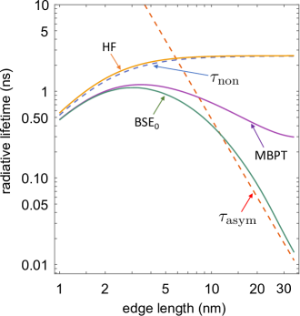
Figure 4: Log-log plot of the radiative lifetime of the $1S_{e}$-$1S_{h}$ ground-state exciton of a NC of CsPbBr₃ vs. NC edge length, in various approximations. All theories assume the EMA. Dashed lines: $\tau_{\text{asym}}$, large-$R$ asymptotic form of the lifetime [Eq. (32)]; $\tau_{\text{non}}$, lifetime for noninteracting particles [Eq. (30)]. Continuous lines (top to bottom): HF, configuration-averaged Hartree-Fock; MBPT, many-body perturbation theory up to first order (following Ref. [13]); BSE₀, particle-hole Bethe-Salpeter equation.

The other case is the large-$R$ limit for interacting carriers. Here one makes use of the bound-exciton wave function $\Psi(\mathbf{r}_{e},\mathbf{r}_{h})$ (24) and generalizes the overlap $\langle 1S_{e}|1S_{h}\rangle$ in Eq. (29) to [11]

$$\int\Psi(\mathbf{r}_{e},\mathbf{r}_{h})\delta^{3}(\mathbf{r}_{e}-\mathbf{r}_{h})\,d^{3}\mathbf{r}_{e}d^{3}\mathbf{r}_{h}$$

$$\quad\quad\quad\quad=\psi_{\text{rel}}(\bm{0})\int\psi_{\text{CM}}(\mathbf{r}^{\prime})\,d^{3}\mathbf{r}^{\prime}$$

$$\quad\quad\quad\quad=\frac{2\sqrt{2}}{\pi}\left(\frac{\mu R}{\varepsilon_{\text{in}}}\right)^{3/2}\,,$$ (31)

which gives the large-$R$ asymptotic form of the lifetime [11],

$$\frac{1}{\tau_{\text{asym}}}=\frac{4}{9}\frac{n_{\text{out}}}{c^{3}}f_{\varepsilon}^{2}\left(E_{g}-\frac{\mu}{2\varepsilon_{\text{in}}^{2}}\right)E_{P}\left(\frac{8}{\pi^{2}}\frac{\mu^{3}R^{3}}{\varepsilon_{\text{in}}^{3}}\right)\,.$$ (32)

For large $R$, the lifetime thus goes as $\tau\sim 1/R^{3}$.

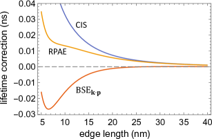
Figure 5: Plot of $\mathbf{k}\cdot\mathbf{p}$ corrections to the lifetime of the $1S_{e}$-$1S_{h}$ ground-state exciton of a NC of CsPbBr₃ vs. NC edge length, for various levels of theory. The $\mathbf{k}\cdot\mathbf{p}$ correction is defined relative to the BSE₀ value (Fig. 4), which corresponds to zero. Continuous curves (top to bottom): CIS, configuration-interaction singles; RPAE, random-phase approximation with exchange; BSE_k⋅p, particle-hole Bethe-Salpeter equation using basis states of the $4\times 4$ $\mathbf{k}\cdot\mathbf{p}$ model.

These analytical results together with various numerical results are shown in Fig. 4 as a function of NC edge length. One sees that the mean-field HF approach gives almost the same lifetime as noninteracting carriers, and both tend to a constant as $L\rightarrow\infty$. Correlation has a large effect as $L$ increases, however. Although MBPT up to first order [13] accounts quite well for the lifetime in the strong-confinement limit $L\ll 2a_{B}=6.1$ nm, it deviates significantly from both BSE₀ and $\tau_{\text{asym}}$ in intermediate confinement and also has the wrong large-$R$ limit [13]. In intermediate confinement, only BSE₀ gives a satisfactory description of the radiative lifetime.

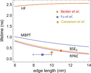
Figure 6: Comparison of theoretical and experimental lifetimes of NCs of CsPbBr₃. Continuous lines (top to bottom): HF, configuration-averaged Hartree-Fock (Ref. [13]); MBPT, many-body perturbation theory up to first order (Ref. [13]); BSE₀, particle-hole Bethe-Salpeter equation using EMA basis states; RPAE, random-phase approximation with exchange using basis states of the $4\times 4$ $\mathbf{k}\cdot\mathbf{p}$ model. Experimental values: Becker et al., Ref. [2]; Fu et al., Ref. [38]; Canneson et al., Ref. [39].

The $\mathbf{k}\cdot\mathbf{p}$ corrections to the radiative lifetime are shown in Fig. 5 using various approaches within the $4\times 4$ $\mathbf{k}\cdot\mathbf{p}$ model. Overall, the $\mathbf{k}\cdot\mathbf{p}$ corrections are small, up to about 5% of the lifetime in intermediate confinement. However, the more complete RPAE approach gives significantly different results from CIS and BSE_k⋅p and, in situations where $\mathbf{k}\cdot\mathbf{p}$ corrections are of interest, is therefore to be preferred.

Our results are compared with the available experimental data (at cryogenic temperatures) in Fig. 6. In the size range of interest, the all-order methods give significantly improved agreement with experiment and bring the theory into good agreement with the measurement of Becker et al. [2]. However, the decay rate is approximately proportional to the Kane parameter $E_{P}$ [see, e.g., Eq. (32)], whose value is presently quite uncertain. A larger value of $E_{P}$ might favor the other measurements. We also note that the measurements disagree with themselves by up to a factor of 2. Further discussion of possible errors in both theory and experiment is given in Ref. [13].

Finally, we note that, in our discussion of the large-$R$ limit of the lifetime [Eq. (32)], we have assumed an idealized situation in which the carriers remain in a single pure quantum state (the ground state) for all NC sizes $R$. For sufficiently large sizes at finite temperature, this assumption will fail and the predicted decrease in lifetime as $1/R^{3}$ will break down [12]. However, Fig. 6 makes it clear that a strong renormalization due to correlation is observable in the experimental data for the synthesized NC sizes at cryogenic temperatures.

III.4 Fine structure: long-range Coulomb interaction

In this section we illustrate the application of all-order methods to the ground-state exciton fine structure, focusing on one contribution, the LR Coulomb interaction (3), which has received much attention recently [40, 18, 41, 19]. Other contributions to the fine structure (with comparable size) include the SR Coulomb interaction (4) [2, 18, 41, 19], NC shape and lattice deformations [40, 18, 41], and a possible strong Rashba interaction [2, 18, 42].

The leading Coulomb contribution to exciton fine structure is the exchange interaction, Figs. 2(c) and (d) [23, 26]. As discussed in Sec. II, this term is formally of order $O[(\mathbf{k}\cdot\mathbf{p})^{2}]$ in $\mathbf{k}\cdot\mathbf{p}$ perturbation theory. In the present approach, $\mathbf{k}\cdot\mathbf{p}$ corrections enter via the small components of the wave function in VB-CB-coupled methods such as the $4\times 4$ $\mathbf{k}\cdot\mathbf{p}$ model. By keeping track of both large and small components when evaluating Coulomb matrix elements, the $\mathbf{k}\cdot\mathbf{p}$ corrections then propagate “automatically” to the final energy. It is thus possible to extract the fine-structure contribution directly by taking the difference of the total energy for the $F_{\text{tot}}=1$ and $F_{\text{tot}}=0$ fine-structure states of the ground-state exciton, testing this difference carefully for numerical significance.

In Fig. 7, we show the LR fine-structure contribution calculated this way in various many-body approximations as a function of NC size. A positive value of the fine structure indicates that the $F_{\text{tot}}=1$ state is higher in energy than the $F_{\text{tot}}=0$ state. Note that the only all-order method shown in the figure is CIS. The BSE_k⋅p method does not reproduce the fine structure accurately. This happens because BSE_k⋅p (like BSE₀) excludes the last term in Eq. (11) [Fig. 1(e)], which is the term that generates the exchange energy [Figs. 2(c) and (d)]. The RPAE method does include this term, but the additional fine-structure $\mathbf{k}\cdot\mathbf{p}$ corrections contained in RPAE relative to CIS are very small, giving a modification of only about 1% or less of the CIS result over the range of sizes shown. As with the radiative lifetime, correlation is seen to be a very important effect in intermediate confinement, and the all-order CIS or RPAE methods give significantly different results from HF and MBPT in this regime.

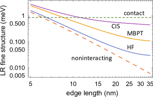
Figure 7: Log-log plot of LR fine structure for a NC of CsPbBr₃ vs. NC edge length, in various approximations. All approaches use the $4\times 4$ $\mathbf{k}\cdot\mathbf{p}$ model. Dashed lines (top to bottom): ‘contact’, large-$R$ asymptotic value calculated assuming an effective contact interaction, Eqs. (33) and (35); ‘noninteracting’, noninteracting carriers, Eq. (34). Continuous lines (top to bottom): CIS, configuration-interaction singles; MBPT, many-body perturbation theory up to first order; HF, configuration-averaged Hartree-Fock. The curve for RPAE is indistinguishable from that for CIS, while BSE_k⋅p accounts poorly for the LR fine structure and is not shown (see text for further discussion).

As before, it is possible to make analytical progress in two cases within the EMA. Using external-leg wave-function corrections to first order in $\mathbf{k}\cdot\mathbf{p}$ perturbation theory, it can be shown [26, 43, 44] that the lowest-order exchange energy, Fig. 2(c), is given in a spherical approximation by the matrix element of the effective contact interaction,

$$\tilde{g}_{12}=\frac{4\pi}{3}\frac{1}{\varepsilon_{\text{in}}\omega_{\alpha}^{2}}\delta^{3}(\mathbf{r}_{1}-\mathbf{r}_{2})\mathbf{p}_{1}\cdot\mathbf{p}_{2}\,.$$ (33)

Here, $\omega_{\alpha}$ is the exciton energy, $\delta^{3}(\mathbf{r}_{1}-\mathbf{r}_{2})$ acts only on the envelope wave functions, and $\mathbf{p}_{1}\cdot\mathbf{p}_{2}$ acts only on the Bloch functions. The operator (33) is strictly valid only when the external states in Fig. 2(c) are $S$ states. For external states of higher angular momentum, a second term with quadrupole symmetry in principle also contributes [44].

Evaluating the matrix element $\langle eh|\tilde{g}_{12}|he\rangle$ using the noninteracting $1S_{e}$ and $1S_{h}$ wave functions (21) gives the LR fine structure for noninteracting particles [19, 18]

$$\mathcal{F}_{\text{non}}=\frac{4\pi}{9}\frac{E_{P}}{\varepsilon_{\text{in}}}\left(E_{g}+\frac{\pi^{2}}{2\mu R^{2}}\right)^{-2}\frac{\xi}{R^{3}}\,,$$ (34)

where $\xi\approx 0.672$1. We can use this expression to test our numerics, by comparing $\mathcal{F}_{\text{non}}$ with the fine structure calculated numerically from the lowest-order exchange diagram, Fig. 2(c), using noninteracting $1S$ states on the external legs that were generated numerically in the $4\times 4$ $\mathbf{k}\cdot\mathbf{p}$ model (including large and small components). We find agreement with Eq. (34) to about one part in $10^{4}$ for large $R$. This exercise fails when the external states have orbital angular momentum greater than zero, because the effective operator in Eq. (33) excludes the quadrupole term.

An estimate of the LR fine structure in the large-$R$ limit can also be made, by evaluating the expectation value $\langle\Psi|\tilde{g}_{12}|\Psi\rangle$ using the bound-exciton wave function $\Psi$ in Eq. (24). This yields

$$\mathcal{F}_{\text{asym}}=\frac{4\pi}{9}\frac{E_{P}}{\varepsilon_{\text{in}}}\left(E_{g}-\frac{\mu}{2\varepsilon_{\text{in}}^{2}}\right)^{-2}\left(\frac{1}{\pi}\frac{\mu^{3}}{\varepsilon_{\text{in}}^{3}}\right)\,.$$ (35)

$\mathcal{F}_{\text{asym}}$ is a constant, representing the LR fine-structure contribution of the bulk exciton, with a value $\mathcal{F}_{\text{asym}}=0.869$ meV for the parameters in Table 1. However, Eq. (35) is only approximate, because the derivation implicitly assumes external states with angular momentum greater than zero on the external legs of the effective operator $\tilde{g}_{12}$ (33). This can be seen by expressing the diagram in Fig. 2(d) in terms of all-order CI amplitudes (6),

$$\mathcal{F}_{\alpha}=\sum_{ehe^{\prime}h^{\prime}}(\mathcal{X}_{e^{\prime}h^{\prime}}^{\alpha})^{*}\mathcal{X}_{eh}^{\alpha}\langle e^{\prime}h|g_{12}|h^{\prime}e\rangle\,.$$ (36)

The sum here is over all exciton channels $(e,h)$ and $(e^{\prime},h^{\prime})$, implying contributions from $P$, $D$, etc., states in the Coulomb matrix element.

A numerical estimate of the large-$R$ limit can instead be made using the all-order CIS method, which is set up to handle the angular couplings in full generality. From Fig. 7, one sees that the LR fine structure is not quite asymptotic (constant) at $L=35$ nm and has a numerical value that is of the same order of magnitude as $\mathcal{F}_{\text{asym}}$, but about half the size.

As mentioned in Sec. II, the contribution of the SR Coulomb interaction to the exciton fine structure is also formally of order $O[(\mathbf{k}\cdot\mathbf{p})^{2}]$, and studies have shown that the SR and LR fine-structure contributions are comparable [18, 19, 40]. The leading SR fine-structure term can be included in the CIS and RPAE approaches by putting $g_{12}=g_{12}^{\text{LR}}+g_{12}^{\text{SR}}$ in the exchange term $\langle eh^{\prime}|g_{12}|he^{\prime}\rangle$ [Fig. 1(e)] in Eq. (11). The $O(1)$ particle-hole ladder terms, generated by iterating Fig. 1(d), will then provide the vertex-renormalization terms in Fig. 2(d), which are also important for the SR fine structure.

III.5 One-photon absorption cross section

The one-photon absorption cross section for laser frequency $\omega$ can be written [45, 11]

$$\sigma^{(1)}(\omega)=\sum_{\alpha}T_{\alpha}^{(1)}\Delta_{\alpha}(\omega-\omega_{\alpha})\,,$$ (37)

where $T_{\alpha}^{(1)}$ is the one-photon “transition strength” to a final-state exciton $\alpha$ with energy $\omega_{\alpha}$, and $\Delta_{\alpha}(\omega-\omega_{\alpha})$ is a line-shape function for this transition. The transition strength is given by

$$T_{\alpha}^{(1)}=\frac{4\pi^{2}}{3}\frac{f_{\varepsilon}^{2}}{n_{\text{out}}c\omega}\left|M_{\alpha}\right|^{2}\,,$$ (38)

involving the same quantities as Eq. (27).

To evaluate Eq. (37), we extract a large number of correlated exciton states $\alpha$ using the CIS (8) or RPAE (13) eigenvalue equations, from the ground state up to a high energy cutoff (typically a few hundred eigenstates up to an excitation energy of several eV). The computed transition strengths $T_{\alpha}^{(1)}$ are then broadened using the phenomenological approach of Ref. [13] (which should be consulted for more details). A Gaussian line-shape function is chosen emphasizing inhomogeneous broadening mechanisms,

$$\Delta_{\alpha}(\omega-\omega_{\alpha})=\frac{1}{\sigma_{\alpha}\sqrt{2\pi}}\exp\left[-\frac{(\omega-\omega_{\alpha})^{2}}{2\sigma_{\alpha}^{2}}\right]\,,$$ (39)

with width parameters

$$\sigma_{\alpha}^{2}=\left(\sigma_{\alpha}^{\text{size}}\right)^{2}+\left(\sigma_{\alpha}^{\text{other}}\right)^{2}\,.$$ (40)

The width $\sigma_{\alpha}^{\text{size}}$ is a transition-dependent term representing the range of NC sizes present in the ensemble, which we take as $\delta L/L\approx 5$% for CsPbBr₃ [9]. Other broadening mechanisms are represented by $\sigma_{\alpha}^{\text{other}}$, which is given the constant value 80 meV for all transitions except the ground-state exciton, for which we take $\sigma_{\alpha}^{\text{other}}=52$ meV. Because the line-shape functions are normalized to unity, $\int_{0}^{\infty}\Delta_{\alpha}(\omega-\omega_{\alpha})\,d\omega=1$, the broadening parameters do not change significantly the average value of the computed cross section $\sigma^{(1)}$, only the appearance of substructure related to individual transitions $T_{\alpha}^{(1)}$. The broadening parameters above, which are physically reasonable, were chosen to reproduce approximately the resolution of individual transitions observed in the experimental absorption spectra of Ref. [9] for an edge length of $L=9.4$ nm (see inset to Fig. 8).

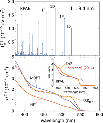
Figure 8: One-photon absorption for a NC of CsPbBr₃ with edge length $L=9.4$ nm. Upper panel: Transition strengths $T_{\alpha}^{(1)}$, Eq. (38), calculated within RPAE using the $8\times 8$ $\mathbf{k}\cdot\mathbf{p}$ model. The quantum numbers of some dominant transitions are indicated; $1S$ indicates a final-state exciton $1S_{e}$-$1S_{h}$, $1P$ indicates $1P_{e}$-$1P_{h}$, etc. Lower panel: continuous lines show one-photon absorption cross sections $\sigma^{(1)}$ calculated in various approximations. HF: configuration-averaged Hartree-Fock; MBPT: many-body perturbation theory up to first order (following Ref. [13]); BSE_k⋅p: particle-hole Bethe-Salpeter approach using single-particle states from the $8\times 8$ $\mathbf{k}\cdot\mathbf{p}$ model. The dashed line, which is nearly coincident with the BSE_k⋅p line, indicates the RPAE approximation. Inset of lower panel: unnormalized one-photon absorption cross section (arbitrary units) taken from the experiment of Chen et al. [9] for a NC of edge length $L=9.4$ nm. The experimental absorption cross section is scaled so that the threshold peak ($1S_{e}$-$1S_{h}$) has the same numerical value as the theoretical BSE_k⋅p curve.

A study of excitons at cryogenic temperatures in bulk (CH₃NH₃)PbBr₃ [46], which may be expected to have a similar band structure to CsPbBr₃, showed a sharp absorption line at an excitation energy of 1.07 eV above threshold. This was attributed to transitions from the $s$-like VB ($R_{6}^{+})$ to the $p_{3/2}$-like CB ($R_{8}^{-})$ at the $R$ point of the Brillouin zone; higher-lying structures around 1.6 eV above threshold were attributed to transitions to the $p_{1/2}$-like CB at the $M$ point. The absorption spectra of NCs of CsPbBr₃ [10, 9] show analogous features in the form of steps in the absorption cross section, the first occurring around 0.6–0.8 eV above threshold (e.g., see the inset to Fig. 8). Interpreted as the threshold for absorption to the $p_{3/2}$-like CB band at the $R$ point ($R_{6}^{+}\rightarrow R_{8}^{-}$), this implies a value of about 0.6–0.8 eV for the spin-orbit coupling parameter $\Delta_{\text{soc}}$ discussed in Sec. III.1 (with small corrections due to the confinement shifts present in the NC spectra, which have an order of magnitude of several tens of meV for an edge length of 9 nm, as shown in Fig. 3). DFT calculations for CsPbBr₃ [2, 18] show a similar energy ordering of band-structure features to that observed for (CH₃NH₃)PbBr₃ in Ref. [46], although the predicted value of $\Delta_{\text{soc}}$ is somewhat larger (e.g., $\Delta_{\text{soc}}=1.54$ eV in Ref. [18]).

For this calculation, we use the $8\times 8$ $\mathbf{k}\cdot\mathbf{p}$ model discussed in Sec. III.1 in order to include the secondary absorption threshold to the $p_{3/2}$-like CB, assuming $\Delta_{\text{soc}}=0.8$ eV. The $8\times 8$ $\mathbf{k}\cdot\mathbf{p}$ model also involves Luttinger parameters $\gamma_{i}$ ($i=1$–3) [21], which describe the effective-mass and intraband couplings within the $p_{3/2}$-like CB. The Luttinger parameters are not known for CsPbBr₃; we choose $\gamma_{i}$ such that $\tilde{\gamma}_{i}=0$, where $\tilde{\gamma}_{i}$ is the contribution to $\gamma_{i}$ from remote bands (not included in the $8\times 8$ $\mathbf{k}\cdot\mathbf{p}$ model). Transition strengths obtained using RPAE are shown in Fig. 8 (upper panel). The first few dominant transitions are to excitons of the form $1l_{e}$-$1l_{h}$ (where $l$ denotes orbital angular momentum), which give nonzero overlaps $\langle 1l_{e}|1l_{h}\rangle$ in Eq. (29) for the noninteracting case. However, correlation and $\mathbf{k}\cdot\mathbf{p}$ corrections allow numerous other transitions with reduced strength, such as $2S_{e}$-$1S_{h}$, which add to the overall absorption strength. Also, a line such as $1P_{e}$-$1P_{h}$ has a small fine structure, with components $1(P_{1/2})_{e}$-$1(P_{1/2})_{h}$, $1(P_{3/2})_{e}$-$1(P_{1/2})_{h}$, $1(P_{1/2})_{e}$-$1(P_{3/2})_{h}$, and $1(P_{3/2})_{e}$-$1(P_{3/2})_{h}$.

Theoretical absorption cross sections after line broadening are shown in the lower panel of Fig. 8 and compared to the experimental cross section of Chen et al. [9] for a NC of edge length 9.4 nm. As discussed in Ref. [13], measurements of the absolute cross section, which have been performed in some cases for particular wavelengths, disagree with each other by up to an order of magnitude. We therefore focus here on the shape of the absorption curve. The all-order cross sections from BSE_k⋅p and RPAE are found to be in good qualitative agreement with the measured cross section of Ref. [9]. Similar agreement is found with Ref. [10], where the absorption curve for $L=9.2$ nm has a similar shape near threshold, with a step around 0.6 eV above threshold. The threshold peak (at about 510 nm) is a transition to the $1S_{e}$-$1S_{h}$ exciton. A weaker transition around 470 nm is just visible in the experimental (and theoretical) curve, and is due mainly to a combination of the $1P_{e}$-$1P_{h}$, $1D_{e}$-$1D_{h}$, and $1F_{e}$-$1F_{h}$ transitions. The secondary transition to the $p_{3/2}$-like CB (around 410 nm) is perhaps more pronounced in the theoretical curve than in the measurement. The strength of this transition relative to the threshold transition is fixed in our approach by the $8\times 8$ $\mathbf{k}\cdot\mathbf{p}$ model, in which the $4\times 4$ $\mathbf{k}\cdot\mathbf{p}$ model is embedded with the ratios of coupling constants constrained by symmetry. However, the ratio of the cross section at 375 nm to its value at the threshold peak is in good agreement with experiment.

Note that the theoretical $1S_{e}$-$1S_{h}$ threshold peak, which is based on a band gap measured at cryogenic temperatures (Table 1), is redshifted by about 0.1 eV compared to the experimental peak, which was measured at room temperature or above. This is likely due to the temperature-dependent shift of the band gap and possibly also to a change of crystal phase [33]. A better fit to the experiment could have been found by choosing $E_{g}$ to be about 0.1 eV larger, compensated by a value of $\Delta_{\text{soc}}$ that is about 0.1 eV smaller, so that the step in the absorption curve occurs at the same wavelength.

Table 3: Transition strengths and renormalization factors for the principal one-photon-absorption transitions in Fig. 8. The columns HF, MBPT (1st-order), and RPAE give the transition strengths summed over fine-structure components, Eq. (41), for the indicated model (units: $10^{-15}$ eV cm²). The renormalization factors $\beta_{\text{MBPT}}$ and $\beta_{\text{RPAE}}$ are the enhancement of the transition strength relative to the HF model.

Transition	HF	MBPT	RPAE	$\beta_{\text{MBPT}}$	$\beta_{\text{RPAE}}$
1S	$0.21$	$0.66$	$1.02$	$3.1$	$4.8$
1P	$0.58$	$1.46$	$1.38$	$2.5$	$2.4$
1D	$0.88$	$2.00$	$1.75$	$2.3$	$2.0$
1F	$1.12$	$2.09$	$1.73$	$1.9$	$1.6$

In Fig. 8, the cross section for HF can be seen to be qualitatively different, rising steadily from a weak threshold peak. The cross section obtained using 1st-order MBPT [13] is a partial improvement on the HF cross section. To understand this phenomenon in more detail, we consider the transition strength of the first few dominant transitions in the various approaches. We find that the various many-body treatments tend to redistribute the transition strength among the fine-structure components in different ways. Since the fine-structure lines are nearly coincident and only the sum of their transition strengths contributes to the observable cross section, for this analysis we therefore sum the transition strength over fine-structure components,

$$\tilde{T}_{\alpha}^{(1)}=\sum_{F,F^{\prime}}T_{\alpha}^{(1)}(F,F^{\prime})\,.$$ (41)

Summed transition strengths are given in Table 3. We also give the enhancement or renormalization factor $\beta$ due to correlation, which is defined as the ratio of $\tilde{T}_{\alpha}^{(1)}$ in a given many-body approach to its value at HF level.

The renormalization factor for the threshold $1S_{e}$-$1S_{h}$ transition is large, about 4.8 for $L=9.4$ nm, and increases further (approximately as $L^{3}$) for larger $L$. This is the same enhancement factor that applies to the radiative decay rate of the ground-state exciton discussed in Sec. III.3. However, as emphasized in Ref. [13], the renormalization factor decreases rapidly with increasing energy, approaching unity. In fact, while 1st-order MBPT underestimates the $1S_{e}$-$1S_{h}$ enhancement factor, it overestimates slightly the factor for the excited-state transitions. The effect of this is that the absorption cross section in an all-order approach tends to have a more prominent threshold peak, followed by a “leveling out” of the cross section at higher energies, bringing the shape of the absorption cross section into better agreement with experiment.

IV Conclusions

We have presented various many-body formalisms, within a $\mathbf{k}\cdot\mathbf{p}$ envelope-function approach, for treating all-order correlated single excitons in NC quantum dots. These formalisms apply both to the EMA and to $\mathbf{k}\cdot\mathbf{p}$ models in which the VB and CB are coupled, such as the $4\times 4$ $\mathbf{k}\cdot\mathbf{p}$ model. The latter allow one to treat the “$\mathbf{k}\cdot\mathbf{p}$ corrections” to the EMA. The simplest many-body approach, valid to order $O(1)$ in $\mathbf{k}\cdot\mathbf{p}$ perturbation theory, was BSE₀ using an EMA basis set. The most complete treatment of $\mathbf{k}\cdot\mathbf{p}$ corrections was given by RPAE. The various formalisms were explicitly adapted to spherical symmetry and expressed in terms of radial integrals and angular factors. The resulting approaches are very rapid and accurate for systems in intermediate confinement, where correlation effects are in general strong (the methods typically require a few seconds of computation time on a single core).

To illustrate these techniques, we considered a class of semiconductor NCs of great recent interest, inorganic lead-halide perovskites such as CsPbBr₃. The most commonly synthesized size range of these NCs corresponds to intermediate confinement. We showed that in this size range, the all-order methods gave significant improvements in accuracy compared to mean-field methods (HF) or to perturbative methods (MBPT to first or second order), and were significantly more accurate also than asymptotic results that can be derived analytically for the infinite-size limit. This was shown to be true for the correlation energy, the radiative lifetime of the ground-state exciton, and the LR Coulomb contribution to the exciton fine structure. Partly as a test of our methods, we also checked that the all-order formalism had the expected large-size limit, where this was known.

The all-order correlation formalism allows one to generate correlated excited states rigorously. We used excited states to investigate the one-photon absorption cross section, where the all-order methods were shown to give a significant improvement in the shape of the cross section (versus laser wavelength) near and just above threshold. Also, because the $\mathbf{k}\cdot\mathbf{p}$ corrections are integrated directly into the all-order formalism for VB-CB-coupled models, the approach allows one to calculate the LR exciton fine structure, an order $O[(\mathbf{k}\cdot\mathbf{p})^{2}]$ effect, by direct subtraction of the total energy of the fine-structure levels. In other problems, such as the exciton correlation energy or lifetime, the $\mathbf{k}\cdot\mathbf{p}$ corrections were found to be quite small (e.g., up to about 5% for the lifetime). However, it was shown that, in situations where these $\mathbf{k}\cdot\mathbf{p}$ corrections are interesting, the more complete RPAE method can give significantly different $\mathbf{k}\cdot\mathbf{p}$ corrections than the other methods, such as BSE_k⋅p, and RPAE is therefore to be preferred.

We considered only single excitons in this paper. Other excitonic systems, such as trions or biexcitons, can be treated by generalized CI approaches [15, 16] or quantum Monte Carlo [15].

*

Appendix A Angular reduction

In this Appendix, we give the reduction of the all-order equations to radial integrals and angular factors for a spherically symmetric potential $V_{\text{ext}}+U$ [Eq. (5)]. The basis states $|e\rangle$ and $|h\rangle$ have definite total angular momentum $F_{e}$ and $F_{h}$ arising from a coupling of orbital, spin, and Bloch band angular momenta [22]; $F_{e}$ and $F_{h}$ couple in turn to a definite total angular momentum $F_{\text{tot}}$ (and parity) for each exciton state. (Here, $F_{e}$ and $F_{h}$ are half-integers and $F_{\text{tot}}$ is an integer.)

It follows that the amplitudes $\mathcal{X}_{eh}^{\alpha}$ and $\mathcal{Y}_{eh}^{\alpha}$ in Eqs. (8) and (13) can be expressed in terms of Clebsch-Gordon coefficients and reduced amplitudes $\mathcal{\bar{X}}_{eh}^{\alpha}$ and $\mathcal{\bar{Y}}_{eh}^{\alpha}$, which do not depend on the magnetic substates $m_{e}$ and $m_{h}$ of $e$ and $h$,

$$\mathcal{X}_{eh}^{\alpha} =\sum_{F_{\text{tot}}M_{\text{tot}}}\mathcal{\bar{X}}_{eh}^{\alpha}(F_{\text{tot}})$$

$$\quad\quad\times(-1)^{F_{h}-m_{h}}\langle F_{e}m_{e},F_{h}-m_{h}|F_{\text{tot}}M_{\text{tot}}\rangle\,,$$ (42)

$$\mathcal{Y}_{eh}^{\alpha} =\sum_{F_{\text{tot}}M_{\text{tot}}}\mathcal{\bar{Y}}_{eh}^{\alpha}(F_{\text{tot}})$$

$$\quad\quad\times(-1)^{F_{e}-m_{e}}\langle F_{e}-m_{e},F_{h}m_{h}|F_{\text{tot}}M_{\text{tot}}\rangle\,.$$ (43)

The equation for $\mathcal{X}_{eh}^{\alpha}$ corresponds to the coupling of $e$ and $h$ in Eq. (7) to a total angular momentum $F_{\text{tot}}$, summed over all allowed values of $F_{\text{tot}}$, with the phase factor and minus sign $-m_{h}$ appearing because $h$ is associated with an annihilation operator in Eq. (7) [47]. In the coefficient $\mathcal{Y}_{eh}^{\alpha}$, the roles of $e$ and $h$ are interchanged [for example, see Eq. (17)].

The Coulomb matrix element can also be expressed in terms of a reduced two-body matrix element $X_{K}(abcd)$ [47],

$$\langle ab|g_{12}|cd\rangle=\sum_{K=0}^{\infty}\sum_{M=-K}^{K}(-1)^{F_{a}+F_{b}+K-m_{a}-m_{b}-M}$$

$$\quad\times\left(\begin{matrix}F_{a}&K&F_{c}\\ -m_{a}&M&m_{c}\end{matrix}\right)\left(\begin{matrix}F_{b}&K&F_{d}\\ -m_{b}&-M&m_{d}\end{matrix}\right)X_{K}(abcd)\,,$$ (44)

where $K$ is a multipole that is in practice limited by angular-momentum and parity selection rules. In Refs. [13] and [37], expressions are given for $X_{K}(abcd)$ in terms of the radial functions and the quantum numbers of the states $a$, $b$, $c$, and $d$ in the $4\times 4$ $\mathbf{k}\cdot\mathbf{p}$ and EMA models.

The RPAE eigenvalue equation for reduced amplitudes $\mathcal{\bar{X}}_{eh}^{\alpha}$ and $\mathcal{\bar{Y}}_{eh}^{\alpha}$ is found by substituting Eqs. (42)–(44) into Eq. (13) and summing over magnetic substates using methods of Racah algebra [47]. One finds

$$\left(\begin{array}[]{cc}\bar{A}&\bar{B}\\ \bar{B}&\bar{A}\end{array}\right)\left(\begin{array}[]{c}\bar{\bm{\mathcal{X}}}^{\alpha}\\ \bar{\bm{\mathcal{Y}}}^{\alpha}\end{array}\right)=\omega_{\alpha}\left(\begin{array}[]{cc}1&0\\ 0&-1\end{array}\right)\left(\begin{array}[]{c}\bar{\bm{\mathcal{X}}}^{\alpha}\\ \bar{\bm{\mathcal{Y}}}^{\alpha}\end{array}\right)\,,$$ (45)

where the reduced matrices $\bar{A}$ and $\bar{B}$ are

$$\bar{A}_{eh,e^{\prime}h^{\prime}}(F_{\text{tot}})=(\epsilon_{e}-\epsilon_{h})\delta_{ee^{\prime}}\delta_{hh^{\prime}}$$

$$\quad+\langle e|(-U)|e^{\prime}\rangle\delta_{hh^{\prime}}-\langle h^{\prime}|(-U)|h\rangle\delta_{ee^{\prime}}$$

$$\quad-(-1)^{F_{\text{tot}}+F_{e^{\prime}}+F_{h^{\prime}}}\sum_{K=0}^{\infty}\left\{\begin{matrix}F_{h}&K&F_{h^{\prime}}\\ F_{e^{\prime}}&F_{\text{tot}}&F_{e}\end{matrix}\right\}X_{K}(eh^{\prime}e^{\prime}h)$$

$$\quad-(-1)^{F_{\text{tot}}+F_{e^{\prime}}+F_{h^{\prime}}}\frac{1}{2F_{\text{tot}}+1}X_{F_{\text{tot}}}(eh^{\prime}he^{\prime})\,,$$ (46)

and

$$\bar{B}_{eh,e^{\prime}h^{\prime}}(F_{\text{tot}}) = -\sum_{K=0}^{\infty}\left\{\begin{matrix}F_{h}&K&F_{e^{\prime}}\\ F_{h^{\prime}}&F_{\text{tot}}&F_{e}\end{matrix}\right\}X_{K}(ee^{\prime}h^{\prime}h)$$ (47)

$${}-\frac{1}{2F_{\text{tot}}+1}X_{F_{\text{tot}}}(ee^{\prime}hh^{\prime})\,.$$

The equations for different values of $F_{\text{tot}}$ and parity decouple, giving one eigenvalue equation for each $F_{\text{tot}}$ and parity. A matrix element $\langle a|(-U)|b\rangle$ in Eq. (46) is the matrix element of a radial potential $-U(r)$, implying that $F_{a}=F_{b}$ and that the states $a$ and $b$ have the same parity. Note that the reduced matrices $\bar{A}$ and $\bar{B}$ given by these equations are real and symmetric.

The RPAE normalization condition (16) becomes

$$\sum_{eh}\left[|\bar{\mathcal{X}}_{eh}^{\alpha}(F_{\text{tot}})|^{2}-|\bar{\mathcal{Y}}_{eh}^{\alpha}(F_{\text{tot}})|^{2}\right]=1\,,$$ (48)

and the reduced matrix element of a one-body operator $M$ with spherical tensor rank $\kappa$ is given by

$$\langle\alpha(F_{\text{tot}})\|\kern 0.82993ptM\kern 0.59998pt\|0\rangle=\delta(F_{\text{tot}},\kappa)\sum_{eh}\left[\bar{\mathcal{X}}_{eh}^{\alpha}(F_{\text{tot}})\langle e\|\kern 0.82993ptM\kern 0.59998pt\|h\rangle\right.$$

$$\quad\quad\quad\quad\left.{}+(-1)^{F_{e}+F_{h}+\kappa}\,\bar{\mathcal{Y}}_{eh}^{\alpha}(F_{\text{tot}})\langle h\|\kern 0.82993ptM\kern 0.59998pt\|e\rangle\right]\,.$$ (49)

An important case is the momentum operator, $M=p$, which arises in interband absorption and emission [20]. Expressions for $\langle a\|\kern 0.82993ptp\kern 0.59998pt\|b\rangle$ in the $4\times 4$ $\mathbf{k}\cdot\mathbf{p}$ model (and in the EMA) are given in Appendix A of Ref. [13], in the form of radial integrals and angular factors, and including all $\mathbf{k}\cdot\mathbf{p}$ corrections arising from the small and large components of the wave functions. In one-photon absorption, the selection rule in Eq. (49) becomes $\delta(F_{\text{tot}},1)$, corresponding to the conservation of angular momentum for absorption of a photon from the NC ground state.

In the CIS approach, only the $\bar{A}$ matrix enters and the reduced eigenvalue equation becomes

$$\bar{A}\,\bar{\bm{\mathcal{X}}}^{\alpha}=\omega_{\alpha}\bar{\bm{\mathcal{X}}}^{\alpha}\,.$$ (50)

The BSE formalism is obtained as usual from the CIS formalism by dropping the last term in Eq. (46). In CIS and BSE, the normalization and reduced matrix elements are given by Eqs. (48) and (49), respectively, with $\bar{\mathcal{Y}}_{eh}^{\alpha}=0$.

References

- Protesescu et al. [2015] L. Protesescu, S. Yakunin, M. I. Bodnarchuk, F. Krieg, R. Caputo, C. H. Hendon, R. X. Yang, A. Walsh, and M. V. Kovalenko, Nanocrystals of cesium lead halide perovskites (CsPbX3, X = Cl, Br, and I): Novel optoelectronic materials showing bright emission with wide color gamut, Nano Lett. 15, 3692 (2015).
- Becker et al. [2018] M. A. Becker, R. Vaxenburg, G. Nedelcu, P. C. Sercel, A. Shabaev, M. J. Mehl, J. G. Michopoulos, S. G. Lambrakos, N. Bernstein, J. L. Lyons, T. Stöferle, R. F. Mahrt, M. V. Kovalenko, D. J. Norris, G. Rainò, and A. L. Efros, Bright triplet excitons in caesium lead halide perovskites, Nature 553, 189 (2018).
- Chaudhary et al. [2021] B. Chaudhary, Y. K. Kshetri, H. S. Kim, S. W. Lee, and T. H. Kim, Current status on synthesis, properties and applications of CsPbX3 (X = Cl, Br, I) perovskite quantum dots/nanocrystals, Nanotechnology 32, 502007 (2021).
- Li et al. [2016] G. R. Li, F. W. R. Rivarola, N. J. L. K. Davis, S. Bai, T. C. Jellicoe, F. de la Pena, S. C. Hou, C. Ducati, F. Gao, R. H. Friend, N. C. Greenham, and Z. K. Tan, Highly efficient perovskite nanocrystal light-emitting diodes enabled by a universal crosslinking method, Adv. Mater. 28, 3528 (2016).
- Deng et al. [2016] W. Deng, X. Z. Xu, X. J. Zhang, Y. D. Zhang, X. C. Jin, L. Wang, S. T. Lee, and J. S. Jie, Organometal halide perovskite quantum dot light-emitting diodes, Adv. Funct. Mater. 26, 4797 (2016).
- Yakunin et al. [2015] S. Yakunin, L. Protesescu, F. Krieg, M. I. Bodnarchuk, G. Nedelcu, M. Humer, G. De Luca, M. Fiebig, W. Heiss, and M. V. Kovalenko, Low-threshold amplified spontaneous emission and lasing from colloidal nanocrystals of caesium lead halide perovskites, Nat. Commun. 6, 8056 (2015).
- Pan et al. [2015] J. Pan, S. P. Sarmah, B. Murali, I. Dursun, W. Peng, M. R. Parida, J. Liu, L. Sinatra, N. Alyami, C. Zhao, E. Alarousu, T. K. Ng, B. S. Ooi, O. M. Bakr, and O. F. Mohammed, Air-stable surface-passivated perovskite quantum dots for ultra-robust, single- and two-photon-induced amplified spontaneous emission, J. Phys. Chem. Lett. 6, 5027 (2015).
- Utzat et al. [2019] H. Utzat, W. W. Sun, A. E. K. Kaplan, F. Krieg, M. Ginterseder, B. Spokoyny, N. D. Klein, K. E. Shulenberger, C. F. Perkinson, M. V. Kovalenko, and M. G. Bawendi, Coherent single-photon emission from colloidal lead halide perovskite quantum dots, Science 363, 1068 (2019).
- Chen et al. [2017] J. S. Chen, K. Zidek, P. Chabera, D. Z. Liu, P. F. Cheng, L. Nuuttila, M. J. Al-Marri, H. Lehtivuori, M. E. Messing, K. L. Han, K. B. Zheng, and T. Pullerits, Size- and wavelength-dependent two-photon absorption cross-section of CsPbBr3 perovskite quantum dots, J. Phys. Chem. Lett. 8, 2316 (2017).
- Brennan et al. [2017] M. C. Brennan, J. E. Herr, T. S. Nguyen-Beck, J. Zinna, S. Draguta, S. Rouvimov, J. Parkhill, and M. Kuno, Origin of the size-dependent Stokes shift in CsPbBr3 perovskite nanocrystals, J. Am. Chem. Soc. 139, 12201 (2017).
- Efros and Efros [1982] A. L. Efros and A. L. Efros, Interband absorption of light in a semiconductor sphere, Sov. Phys. Semicond. 16, 772 (1982).
- Takagahara [1987] T. Takagahara, Excitonic optical nonlinearity and exciton dynamics in semiconductor quantum dots, Phys. Rev. B 36, 9293 (1987).
- Nguyen et al. [2020a] T. P. T. Nguyen, S. A. Blundell, and C. Guet, One-photon absorption by inorganic perovskite nanocrystals: A theoretical study, Phys. Rev. B 101, 195414 (2020a).
- Chang and Xia [1998] K. Chang and J. B. Xia, Spatially separated excitons in quantum-dot quantum well structures, Phys. Rev. B 57, 9780 (1998).
- Shumway et al. [2001] J. Shumway, A. Franceschetti, and A. Zunger, Correlation versus mean-field contributions to excitons, multiexcitons, and charging energies in semiconductor quantum dots, Phys. Rev. B 63, 155316 (2001).
- Tyrrell and Tomic [2015] E. J. Tyrrell and S. Tomic, Effect of correlation and dielectric confinement on excitons in CdTe/CdSe and CdSe/CdTe type-II quantum dots, J. Phys. Chem. C 119, 12720 (2015).
- Nguyen et al. [2020b] T. P. T. Nguyen, S. A. Blundell, and C. Guet, Calculation of the biexciton shift in nanocrystals of inorganic perovskites, Phys. Rev. B 101, 125424 (2020b).
- Sercel et al. [2019a] P. C. Sercel, J. L. Lyons, D. Wickramaratne, R. Vaxenburg, N. Bernstein, and A. L. Efros, Exciton fine structure in perovskite nanocrystals, Nano Lett. 19, 4068 (2019a).
- Tamarat et al. [2019] P. Tamarat, M. I. Bodnarchuk, J.-B. Trebbia, R. Erni, M. V. Kovalenko, J. Even, and B. Lounis, The ground exciton state of formamidinium lead bromide perovskite nanocrystals is a singlet dark state, Nat. Mater. 18, 717 (2019).
- Kira and Koch [2012] M. Kira and S. W. Koch, Semiconductor Quantum Optics (Cambridge University Press, New York, 2012).
- Efros and Rosen [2000] A. L. Efros and M. Rosen, The electronic structure of semiconductor nanocrystals, Annu. Rev. Mater. Sci. 30, 475 (2000).
- Ekimov et al. [1993] A. I. Ekimov, F. Hache, M. C. Schanneklein, D. Ricard, C. Flytzanis, I. A. Kudryavtsev, T. V. Yazeva, A. V. Rodina, and A. L. Efros, Absorption and intensity-dependent photoluminescence measurements on CdSe quantum dots—assignment of the 1st electronic-transitions, J. Opt. Soc. Am. B 10, 100 (1993).
- Knox [1963] R. S. Knox, Theory of Excitons, edited by F. Seitz and D. Turnbull, Solid State Physics, Supplement 5 (Academic, New York, 1963).
- Jackson [1998] J. D. Jackson, Classical Electrodynamics, 3rd ed. (Wiley, New York, 1998).
- Karpulevich et al. [2019] A. Karpulevich, H. Bui, Z. Wang, S. Hapke, C. P. Ramirez, H. Weller, and G. Bester, Dielectric response function for colloidal semiconductor quantum dots, J. Chem. Phys. 151, 224103 (2019).
- Pikus and Bir [1971] G. E. Pikus and G. L. Bir, Exchange interaction in excitons in semiconductors, Zh. Eksp. Teor. Fiz. 60, 195 (1971).
- Sercel et al. [2019b] P. C. Sercel, J. L. Lyons, N. Bernstein, and A. L. Efros, Quasicubic model for metal halide perovskite nanocrystals, J. Chem. Phys. 151, 234106 (2019b).
- Blundell et al. [2021] S. A. Blundell, T. P. T. Nguyen, and C. Guet, Calculation of two-photon absorption by nanocrystals of , Phys. Rev. B 103, 045415 (2021).
- Mahan [2000] G. D. Mahan, Many-Particle Physics, 3rd ed. (Kluwer Academic/Plenum Publishers, New York, 2000).
- Amusia and Cherepkov [1975] M. Y. Amusia and N. A. Cherepkov, Many-electron correlations in scattering processes, in Case Studies in Atomic Physics, Vol. 5(2) (North-Holland, Amsterdam, 1975) pp. 47–179.
- Guet and Johnson [1992] C. Guet and W. R. Johnson, Dipole excitations of closed-shell alkali-metal clusters, Phys. Rev. B 45, 11283 (1992).
- Even et al. [2014] J. Even, L. Pedesseau, and C. Katan, Analysis of multivalley and multibandgap absorption and enhancement of free carriers related to exciton screening in hybrid perovskites, J. Phys. Chem. C 118, 11566 (2014).
- Yang et al. [2017] Z. Yang, A. Surrente, K. Galkowski, A. Miyata, O. Portugall, R. J. Sutton, A. A. Haghighirad, H. J. Snaith, D. K. Maude, P. Plochocka, and R. J. Nicholas, Impact of the halide cage on the electronic properties of fully inorganic cesium lead halide perovskites, ACS Energy Lett. 2, 1621 (2017).
- Fu et al. [2017a] J. Fu, Q. Xu, G. Han, B. Wu, C. H. A. Huan, M. L. Leek, and T. C. Sum, Hot carrier cooling mechanisms in halide perovskites, Nat. Commun. 8, 1 (2017a).
- Shcherbakov-Wu et al. [2021] W. Shcherbakov-Wu, P. C. Sercel, F. Krieg, M. V. Kovalenko, and W. A. Tisdale, Temperature-independent dielectric constant in CsPbBr3 nanocrystals revealed by linear absorption spectroscopy, J. Phys. Chem. Lett. 12, 8088 (2021).
- Dirin et al. [2016] D. N. Dirin, I. Cherniukh, S. Yakunin, Y. Shynkarenko, and M. V. Kovalenko, Solution-grown CsPbBr3 perovskite single crystals for photon detection, Chem. Mater. 28, 8470 (2016).
- Nguyen [2020] T. P. T. Nguyen, A theoretical study of correlation effects of N electrons in semiconductor nanocrystals: Applications to optoelectronic properties of perovskite nanocrystals, Ph.D. thesis, Univ. Grenoble Alpes, France (2020).
- Fu et al. [2017b] M. Fu, P. Tamarat, H. Huang, J. Even, A. L. Rogach, and B. Lounis, Neutral and charged exciton fine structure in single lead halide perovskite nanocrystals revealed by magneto-optical spectroscopy, Nano Lett. 17, 2895 (2017b).
- Canneson et al. [2017] D. Canneson, E. V. Shornikova, D. R. Yakovlev, T. Rogge, A. A. Mitioglu, M. V. Ballottin, P. C. M. Christianen, E. Lhuillier, M. Bayer, and L. Biadala, Negatively charged and dark excitons in CsPbBr3 perovskite nanocrystals revealed by high magnetic fields, Nano Lett. 17, 6177 (2017).
- Ben Aich et al. [2019] R. Ben Aich, I. Saidi, S. Ben Radhia, K. Boujdaria, T. Barisien, L. Legrand, F. Bernardot, M. Chamarro, and C. Testelin, Bright-exciton splittings in inorganic cesium lead halide perovskite nanocrystals, Phys. Rev. Appl. 11, 034042 (2019).
- Ben Aich et al. [2020] R. Ben Aich, S. Ben Radhia, K. Boujdaria, M. Chamarro, and C. Testelin, Multiband model for tetragonal crystals: Application to hybrid halide perovskite nanocrystals, J. Phys. Chem. Lett. 11, 808 (2020).
- Swift et al. [2021] M. W. Swift, J. L. Lyons, A. L. Efros, and P. C. Sercel, Rashba exciton in a 2D perovskite quantum dot, Nanoscale 13, 16769 (2021).
- Takagahara [1993] T. Takagahara, Effects of dielectric confinement and electron-hole exchange interaction on excitonic states in semiconductor quantum dots, Phys. Rev. B 47, 4569 (1993).
- Tong and Wu [2011] H. Tong and M. W. Wu, Theory of excitons in cubic III-V semiconductor GaAs, InAs and GaN quantum dots: Fine structure and spin relaxation, Phys. Rev. B 83, 235323 (2011).
- Elliott [1957] R. J. Elliott, Intensity of optical absorption by excitons, Phys. Rev. 108, 1384 (1957).
- Tanaka et al. [2003] K. Tanaka, T. Takahashi, T. Ban, T. Kondo, K. Uchida, and N. Miura, Comparative study on the excitons in lead-halide-based perovskite-type crystals CH3NH3PbBr3 CH3NH3PbI3, Solid State Commun. 127, 619 (2003).
- Brink and Satchler [1994] D. M. Brink and G. R. Satchler, Angular Momentum, 3rd ed. (Clarendon Press, Oxford, 1994).