Phase and amplitude evolution in the network of triadic interactions of the Hasegawa-Wakatani system

Abstract

Hasegawa-Wakatani system, commonly used as a toy model of dissipative drift waves in fusion devices is revisited with considerations of phase and amplitude dynamics of its triadic interactions. It is observed that a single resonant triad can saturate via three way phase locking where the phase differences between dominant modes converge to constant values as individual phases increase in time. This allows the system to have approximately constant amplitude solutions. Non-resonant triads show similar behavior only when one of its legs is a zonal wave number. However when an additional triad, which is a reflection of the original one with respect to the $y$ axis is included, the behavior of the resulting triad pair is shown to be more complex. In particular, it is found that triads involving small radial wave numbers (large scale zonal flows) end up transferring their energy to the subdominant mode which keeps growing exponentially, while those involving larger radial wave numbers (small scale zonal flows) tend to find steady chaotic or limit cycle states (or decay to zero). In order to study the dynamics in a connected network of triads, a network formulation is considered including a pump mode, and a number of zonal and non-zonal subdominant modes as a dynamical system. It was observed that the zonal modes become clearly dominant only when a large number of triads are connected. When the zonal flow becomes dominant as a ’collective mean field’, individual interactions between modes become less important, which is consistent with the inhomogeneous wave-kinetic picture. Finally, the results of direct numerical simulation is discussed for the same parameters and various forms of the order parameter are computed. It is observed that nonlinear phase dynamics results in a flattening of the large scale phase velocity as a function of scale in direct numerical simulations.

I Introduction

Two dimensional Hasegawa-Wakatani equations[1] with proper zonal response consist of an equation of plasma vorticity

$$\frac{\partial}{\partial t}\nabla^{2}\Phi+\hat{\mathbf{z}}\times\nabla\Phi\cdot\nabla\nabla^{2}\Phi=C\left(\widetilde{\Phi}-\widetilde{n}\right)+D_{\Phi}\left(\nabla^{2}\Phi\right)$$ (1)

and an equation of continuity

$$\frac{\partial}{\partial t}n+\hat{\mathbf{z}}\times\nabla\Phi\cdot\nabla n+\kappa\partial_{y}\Phi=C\left(\widetilde{\Phi}-\widetilde{n}\right)+D_{n}\left(n\right)\;\text{,}$$ (2)

with the $E\times B$ velocity defined as $\boldsymbol{v}_{E}=\hat{\mathbf{z}}\times\nabla\Phi$ in normalized form and $\widetilde{\Phi}=\Phi-\left\langle\Phi\right\rangle$ where $\left\langle\Phi\right\rangle$ denotes averaging in $y$ (i.e. poloidal) direction. Here $n$ is the fluctuating particle density normalized to a background density $n_{0}$, $\Phi$ is the electrostatic potential normalized to $T/e$, $\kappa$ is the diamagnetic velocity normalized to speed of sound, $C$ is the so called adiabaticity parameter, which is a measure of the electron mobility and $D_{\Phi}$ and $D_{n}$ are dissipation functions for vorticity and particle density respectively. For fluctuations we have $D_{\Phi}\left(\nabla^{2}\widetilde{\Phi}\right)=\nu\nabla^{4}\widetilde{\Phi}$ from kinematic viscosity, whereas for the zonal flows $D_{\Phi}\left(\nabla^{2}\overline{\Phi}\right)=-\nu_{ZF}\nabla^{2}\overline{\Phi}$ from large scale friction. Unless the system represents a renormalized formulation, $D_{n}$ should actually be zero, however here we include it for completeness and numerical convenience and take it to have the same form as the vorticity dissipation with diffusion $D_{n}\left(\widetilde{n}\right)=D\nabla^{2}\widetilde{n}$ and particle loss $D\left(\overline{n}\right)=-D_{ZF}\overline{n}$.

The Hasegawa Wakani model, was initially devised as a simple, nonlinear model of dissipative drift wave turbulence in tokamak plasmas. It has the same nonlinear structure as the passive scalar turbulence [2] -with vorticity evolving according to 2D Navier-Stokes equations- or more complex problems such as rotating convection [3, 4]. From a plasma physics perspective it can be considered as the minimum non-trivial model for plasma turbulence, since it has i) linear instability (e.g. Hasegawa-Mima model does not [5]), ii) finite frequency (so that resonant interactions are possible [6]), and iii) a proper treatment of zonal flows[7]. The model is well known to generate high levels of large scale zonal flows, especially for $C\gtrsim 1$ [8, 9, 10]. It has been studied in detail for many problems in fusion plasmas including dissipative drift waves in tokamak edge [11, 12], subcritical turbulence[13], trapped ion modes [14], intermittency [15, 16], closures [17, 18, 19], feedback control [20], information geometry [21] and machine learning [22]. Variations of the Hasegawa-Wakatani model are regularly used for describing turbulence in basic plasma devices[23, 24, 25].

Formation of large scale structures, in particular Zonal flows in drift wave turbulence is one of the key issues in the study of turbulence in fusion plasmas, which can be formulated in terms of modulational instability of either a gas of drift wave turbulence using the wave kinetic formulation [26] or a small number of drift modes[27], resulting in various forms of complex amplitude equations such as the celebrated nonlinear Schrödinger equation (NLS) [28]. It is also common to talk about zonal flows as resulting from a process of inverse cascade[29, 30]and their back reaction on turbulence[31, 32] results in predator-prey dynamics, possibly leading up to the low to high confinement transition in tokamaks[33, 34]. While the role of the complex phases in nonlinear evolution of the amplitudes, especially in the context of structure formation, for example as in the case of soliton formation in NLS, was always well known, its particular importance for zonal flow formation in toroidal geometry has been underlined recently[35].

Here we revisit the Hasegawa-Wakatani system, with proper zonal response, as a minimum system that allows a description of zonal flow formation in drift wave turbulence, and study interactions between various number of modes from three wave interactions to the full spectrum of modes described by direct numerical simulations, focusing in particular on phase dynamics and the possibility of phase locking and synchronization. It turns out that while resonant three wave interactions involving unstable and damped modes favor phase locking (i.e. a state where the differences between individual phases remain roughly constant as they increase together), interactions involving zonal flows (i.e. four wave interactions including the triad reflected with respect to the $y$ axis), seems to have a complicated set of possible outcomes depending on if the zonal flow wave number is larger or smaller than the pump wave-number. It therefore becomes critical to study a “network” of connected triads in order to see the collective effects of a number of triads on the evolution of zonal flows and of the relative phases between modes. Two different network configurations are considered: that with a single $k_{y}$ and many different $q$’s, and that with a single $q$ but many different $k_{y}$’s. Note that the algorithm that we use computes all possible interactions between the modes in a given collection of triads and then computes the interaction coefficients and evolves the system nonlinearly according to those.

Finally we consider the results from direct numerical simulations (DNS) using a pseudo-spectral 2D Hasegawa-Wakatani solver. The DNS and the network models correspond exactly, in the sense that if we consider an $N_{x}\times N_{y}$ grid and consider all the possible triads in such a grid and solve this problem using our network solver, we obtain exactly the same problem (including the boundary conditions that are periodic) as the DNS. The results of the DNS show qualitatively similar behavior to the two network models that we considered. However looking at the evolution of phases, we observe a nonlinear flattening of the phase velocity for large scales computed as a function of $x$, suggesting nonlinear structure formation in the classical sense of nonlinearity balancing dispersion resulting in a constant velocity propagation at least for large r scale structures. These vortex-like structures that move at a constant velocity are also clearly visible in the time evolution of density and vorticity fields.

The rest of the paper is organized as follows. In the remainder of the introduction, the Hasegawa-Wakatani system is reformulated in terms of its linear eigenmodes and the amplitude and phase equations for these eigenmodes, writing out explicitly the nonlinear terms that appear in this formulation. In Section II, different types of interactions among dissipative drift waves are considered using these linear eigenmodes, starting with the basic three wave interaction. After showing that there is no qualitative difference between a near resonant and an exactly resonant (within numerical accuracy) triad, the details of the phase dynamics of such a single triad are discussed. In Section III, the interaction with zonal flows are considered. It is noted that when we consider a triad and its reflection with respect to its pump wave-number together as a pair, the behavior of the system is qualitatively different from the single triad case. After a discussion of order parameters for this system, a network formulation is considered and the results from such a network model is presented. Finally the reslts from direct numerical simulations of the Hasegawa-Wakatani system is discussed and compared with those earlier results based on reduced number of triads. Section IV is conclusion.

I.1 Linear Eigenmodes

We can write the Hasegawa-Wakatani system in Fourier space for non-zonal modes (i.e. $k_{y}\neq 0$) as follows:

$$\partial_{t}\Phi_{k}+\left(A_{k}-B_{k}\right)\Phi_{k}=\frac{C}{k^{2}}n_{k}+N_{\Phi k}$$ (3)

$$\partial_{t}n_{k}+\left(A_{k}+B_{k}\right)n_{k}=\left(C-i\kappa k_{y}\right)\Phi_{k}+N_{nk}$$ (4)

where

$$A_{k}=\frac{1}{2}\left[\left(Dk^{2}+C\right)+\left(\frac{C}{k^{2}}+\nu k^{2}\right)\right]$$ (5)

and

$$B_{k}=\frac{1}{2}\left[\left(Dk^{2}+C\right)-\left(\frac{C}{k^{2}}+\nu k^{2}\right)\right]\;\text{.}$$ (6)

using the simpler notation $\Phi_{\mathbf{k}}\rightarrow\Phi_{k}$ and defining:

$$N_{nk}=\frac{1}{2}\sum_{\triangle}\hat{\mathbf{z}}\times\mathbf{p}\cdot\mathbf{q}\left(\Phi_{p}^{*}n_{q}^{*}-\Phi_{q}^{*}n_{p}^{*}\right)$$ (7)

and

$$N_{\Phi k}=\frac{1}{2}\sum_{\triangle}\frac{\hat{\mathbf{z}}\times\mathbf{p}\cdot\mathbf{q}\left(q^{2}-p^{2}\right)\Phi_{p}^{*}\Phi_{q}^{*}}{k^{2}}\;\text{.}$$ (8)

Diagonalizing the linear terms we can write:

$$\partial_{t}\xi_{k}^{\pm}+i\omega_{k}^{\pm}\xi_{k}^{\pm}=N_{\xi k}^{\pm}$$ (9)

with the complex eigen-frequencies $\omega_{k}^{\pm}=\omega_{rk}^{\pm}+i\gamma_{k}^{\pm}$ that can be written as:

$$\omega_{k}^{\pm}=\Omega_{k}^{\pm}-iA_{k}$$

with

$$\Omega_{k}^{\pm}=\pm\left(\sigma_{k}\sqrt{\frac{H_{k}-G_{k}}{2}}+i\sqrt{\frac{H_{k}+G_{k}}{2}}\right)$$ (10)

where $\sigma_{k}=\text{sign}\left(\kappa k_{y}\right)$,

$$H_{k}=\sqrt{G_{k}^{2}+C^{2}\kappa^{2}k_{y}^{2}/k^{4}}\;\text{,}$$ (11)

and

$$G_{k}\equiv\left(B_{k}^{2}+\frac{C^{2}}{k^{2}}\right)\;\text{.}$$ (12)

This allows us to write the two linear eigenmodes as:

$$\xi_{k}^{s_{k}}=n_{k}+\frac{k^{2}}{C}\left[B_{k}-i\Omega_{k}^{s_{k}}\right]\Phi_{k}\;\text{.}$$ (13)

where $s_{k}=\pm$. The nonlinear terms in (9) become:

$$N_{\xi k}^{s_{k}}=N_{nk}+\frac{k^{2}}{C}\left(B_{k}-i\Omega_{k}^{s_{k}}\right)N_{\Phi k}\;\text{,}$$ (14)

and the inverse transforms can be written as:

$$\Phi_{k}=\frac{i}{2}\frac{C}{k^{2}}\sum_{s_{k}}\frac{\xi_{k}^{s_{k}}}{\Omega_{k}^{s_{k}}}$$ (15)

$$n_{k}=-\frac{i}{2}\sum_{s_{k}}\frac{1}{\Omega_{k}^{s_{k}}}\left(B_{k}+i\Omega_{k}^{s_{k}}\right)\xi_{k}^{s_{k}}\;\text{.}$$ (16)

Considering the inviscid limit, $\left\{D,\nu\right\}\rightarrow 0$ and $k_{y}\rightarrow O\left(\epsilon\right)$, where we keep terms only up to $O\left(\epsilon\right)$ we obtain:$k$

$$\xi_{k}^{+}=n_{k}+\left(k^{2}-i\frac{\kappa k_{y}}{2A_{k}^{2}}\right)\Phi_{k}$$

$$\xi_{k}^{-}=n_{k}-\left(1+i\frac{\kappa k_{y}}{2A_{k}^{2}}\right)\Phi_{k}\;\text{,}$$

which means that one could loosely refer to these two modes as the potential vorticity mode (i.e. $\xi_{k}^{+}=n_{k}+k^{2}\Phi_{k}$) and the non-adiabatic electron density mode (i.e. $\xi_{k}^{-}=n_{k}-\Phi_{k}$), somewhat similar to the real space decomposition used in Ref. 36. Since the equations are already diagonal for $k_{y}=0$ modes, we can use $\xi_{k}^{+}=k^{2}\Phi_{k}$ and $\xi_{k}^{-}=n_{k}$ for those (or $\overline{\Phi}_{k}$ and $\overline{n}_{k}$ explicitly as we will do below).

Notice that the two eigenmodes in (13) are not orthogonal. They have the same frequencies (in opposite directions) but different growth rates with $\gamma_{k}^{+}>\gamma_{k}^{-}$ (with $\gamma_{k}^{-}<0$, while $\gamma_{k}^{+}$ can be positive or negative depending on the wave-number). The full nonlinear initial value problem can be solved using linear eigenmodes by first computing $\xi_{k}^{s_{k}}\left(0\right)$ from (13), and then advancing those to $\xi_{k}^{s_{k}}\left(t\right)$ using (9), where the linear matrix is now diagonal (but the nonlinear coupling terms are rather complicated), and finally going back to compute $\Phi_{k}\left(t\right)$ and $n_{k}\left(t\right)$ using (15-16). Obviously, this approach does not involve any kind of approximation.

I.2 Amplitude and Phase Equations

Substituting $\xi_{k}^{\pm}=\chi_{k}^{\pm}e^{i\phi_{k}^{\pm}}$ into (9), we get:

$$\partial_{t}\left(\chi_{k}^{\pm}e^{i\phi_{k}^{\pm}}\right)+i\omega_{k}^{\pm}\chi_{k}^{\pm}e^{i\phi_{k}^{\pm}}=\left|N_{\xi k}^{\pm}\right|e^{i\phi_{k}^{N_{\xi\pm}}}\;\text{,}$$ (17)

taking the real part we obtain the amplitude equations:

$$\left(\partial_{t}-\gamma_{k}^{\pm}\right)\chi_{k}^{\pm}=\left|N_{\xi k}^{\pm}\right|\cos\left(\phi_{k}^{N_{\xi\pm}}-\phi_{k}^{\pm}\right)$$ (18)

and taking the imaginary part and dividing by $\chi_{k}^{\pm}$ we get the phase equations:

$$\partial_{t}\phi_{k}^{\pm}=-\omega_{kr}^{\pm}+\frac{\left|N_{\xi k}^{\pm}\right|}{\chi_{k}^{\pm}}\sin\left(\phi_{k}^{N_{\xi\pm}}-\phi_{k}^{\pm}\right)\;\text{.}$$ (19)

The form of the amplitude equation (18) means that the fixed point for the amplitude evolution is determined by the phase difference between $N_{\xi k}^{s_{k}}$ and $\xi_{k}^{s_{k}}$ for each $s_{k}$. However such a fixed point keeps evolving since the phases themselves increase linearly with the linear frequency while being deformed by the nonlinear terms. Note that if the nonlinear phase is dominated by a slowly evolving mean phase (could be the case if the nonlinear interactions are dominated by the theractions with a zonal flow), the individual phases will be attracted to this nonlinear mean phase, since if the individual phase is behind the nonlinear phase, the $\sin\left(\phi_{k}^{N_{\xi\pm}}-\phi_{k}^{\pm}\right)$ will be positive, causing the individual phase to accelerate, whereas if the individual phase is ahead of the nonlinear phase it will be slowed down. However since we have linear frequencies it is impossible for individual phases to become phase locked directly with the slow nonlinear phase. Instead the nonlinear term plays a role akin to that of the ponderomotive force in parametric instability.

I.3 Nonlinear Terms

In order to compute $N_{\xi k}^{\pm}$ in terms of $\xi_{k}^{\pm}$, we need to go back to $\Phi_{k}$ and $n_{k}$ using (15-16), compute the nonlinear terms (7-8) using those and combine them as in (14). They can then be written in the form:

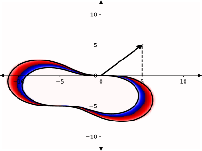
Figure 1: The resonance manifold $\Delta\omega=\omega_{\mathbf{k}r}^{+}+\omega_{\mathbf{p}r}^{+}+\omega_{\mathbf{q}r}^{+}=0$ of the Hasegawa-Wakatani system for the case $C=1.0$, $\kappa=0.2$, $\nu=D=10^{-3}$ is shown corresponding to the wave vector $\mathbf{k}=\left(5,5\right)$ that is shown explicitly. Any $\mathbf{p}$ that falls onto the region inside the resonance manifold (shown here with a finite width of $\pm 0.04$ with $\Delta\omega>0$ in red and $\Delta\omega<0$ in blue if in color) gives $\Delta\omega\approx 0$ (with $\mathbf{q}=-\mathbf{k}-\mathbf{p}$). As discussed in the text, because of the fact that the $\left(+\right)$ and $\left(-\right)$ modes have the same frequency (but opposite direction of propagation in $y$ direction) all possible combinations of $\left(+\right)$ and $\left(-\right)$ modes resonate on the same manifold.

$$N_{\xi k}^{s_{k}}=\frac{1}{2}\sum_{\triangle}\sum_{s_{p},s_{q}}M_{kpq}^{s_{k}s_{p}s_{q}}\xi_{p}^{s_{p}*}\xi_{q}^{s_{p}*}$$ (20)

in terms of the linear eigenmodes, where the sum is over $s_{p},s_{q}=\left\{\left(+,+\right),\left(+,-\right),\left(-,+\right),\left(-,-\right)\right\}$ for $s_{k}=\left(+,-\right)$. The nonlinear interaction coefficients in (20) can be written (i.e. between 3 non-zonal modes) as:

$$M_{\xi kpq}^{s_{k}s_{p}s_{q}} =m_{kpq}^{s_{k}s_{p}s_{q}}\bigg{[}q^{2}\left(B_{q}-i\Omega_{q}^{s_{q}*}\right)$$

$$-p^{2}\left(B_{p}-i\Omega_{p}^{s_{p}*}\right)-\left(q^{2}-p^{2}\right)\left(B_{k}-i\Omega_{k}^{s_{k}}\right)\bigg{]}$$ (21)

where

$$m_{kpq}^{s_{k}s_{p}s_{q}}\equiv\frac{C\hat{\mathbf{z}}\times\mathbf{p}\cdot\mathbf{q}}{4\Omega_{p}^{s_{p}*}\Omega_{q}^{s_{q}*}q^{2}p^{2}}$$

and $\Omega_{k}^{\pm}$ is given in (10).

Note that these coefficients are complex, and have different phases in general. In other words the explicit forms of (19) can be written as:

$$\partial_{t}\phi_{k}^{s_{k}} =-\omega_{kr}^{s_{k}}+\sum_{\triangle}\sum_{s_{p},s_{q}}\frac{\left|M_{\xi kpq}^{s_{k}s_{p}s_{q}}\right|\left|\xi_{p}^{s_{p}}\right|\left|\xi_{q}^{s_{q}}\right|}{\left|\xi_{k}^{s_{k}}\right|}$$

$$\times\sin\left(\theta_{M_{kpq}}^{s_{k}s_{p}s_{q}}-\phi_{p}^{s_{p}}-\phi_{q}^{s_{q}}-\phi_{k}^{s_{k}}\right)$$ (22)

where $\theta_{M_{kpq}}^{s_{k}s_{p}s_{q}}$ is the phase of the nonlinear interaction coefficient $M_{\xi kpq}^{s_{k}s_{p}s_{q}}$.

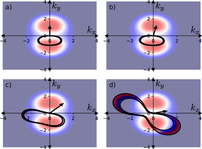
Figure 2: The resonance manifold, shown on top of the growth rate where red corresponds to $\gamma_{\mathbf{k}}^{+}>0$ and blue to $\gamma_{\mathbf{k}}^{+}<0$ for a) the most unstable model on the grid $\mathbf{k}=\left(0,1.125\right)$, b) a nearby mode with a small $k_{x}$ component $\mathbf{k}=\left(0.250,1.125\right)$, c) a mode with $k_{x}=k_{y}$ that is $\mathbf{k}=\left(1.125,1.125\right)$ and finally d) a mode that has $k_{x}\gg k_{y}$ with $\mathbf{k}=\left(1.125,0.125\right)$.

II Interactions among drift waves

II.1 Three wave interactions

Consider three separate modes $k$, $p$ and $q$ that satisfy the triadic interaction condition $\mathbf{k}+\mathbf{p}+\mathbf{q}=0$, possibly in the presence of other modes. The nonlinear term for the wave number $k$ can then be divided into the interaction with the pair $p$ and $q$, and the interaction with the rest of the modes (if they exist). If the three wave interaction that we consider is resonant, slightly off-resonance, or completely non-resonant, its evolution is likely to be different, which can be considered as different scenarios. It may also be possible to model the effects of rest of the modes as background forcing, modification of the linear terms (à la eddy damping) or simply as stochastic noise. Thus separating the nonlinear term into the interaction with the pair $p$ and $q$ (i.e. $N_{\xi kpq}^{\pm}$) and the interaction with the rest of the modes (i.e. $\delta N_{\xi kpq}^{\pm}$), we can write:

$$\partial_{t}\xi_{k}^{\pm}+i\omega_{k}^{\pm}\xi_{k}^{\pm}=N_{\xi kpq}^{\pm}+\delta N_{\xi kpq}^{\pm}$$ (23)

where

$$N_{\xi kpq}^{\pm}= M_{\xi kpq}^{\pm++}\xi_{p}^{+*}\xi_{q}^{+*}+M_{\xi kpq}^{\pm+-}\xi_{p}^{+*}\xi_{q}^{-*}$$

$$+M_{\xi kpq}^{\pm-+}\xi_{p}^{-*}\xi_{q}^{+*}+M_{\xi kpq}^{\pm--}\xi_{p}^{-*}\xi_{q}^{-*}$$

with $M_{\xi kpq}^{\pm\pm\pm}$ being (complex) nonlinear interaction coefficients, and

$$\delta N_{\xi kpq}^{\pm}=N_{\xi k}^{\pm}-N_{\xi kpq}^{\pm}\;\text{.}$$

The $p$ and $q$ modes evolve similarly:

$$\partial_{t}\xi_{p}^{\pm}+i\omega_{p}^{\pm}\xi_{p}^{\pm}=N_{\xi pqk}^{\pm}+\delta N_{\xi pqk}^{\pm}$$ (24)

$$\partial_{t}\xi_{q}^{\pm}+i\omega_{q}^{\pm}\xi_{q}^{\pm}=N_{\xi qkp}^{\pm}+\delta N_{\xi qkp}^{\pm}$$ (25)

Notice that, since there are two eigenmodes (23-25) represent 6 equations. One can therefore consider resonances between $3$ growing modes, $2$ growing modes and a damped mode, or a growing mode and $2$ damped modes etc. However since the frequencies are the same with opposing signs, and due to the condition that the flow field is real, we have both $k_{y}$ and $-k_{y}$ components, whenever we have a resonance say of the form $\omega_{\mathbf{k}}^{+}+\omega_{\mathbf{p}}^{+}+\omega_{\mathbf{q}}^{+}=0$, (with $\mathbf{k}+\mathbf{p}+\mathbf{q}=0$), we also have $\omega_{\mathbf{k}}^{-}+\omega_{\mathbf{p}}^{-}+\omega_{\mathbf{q}}^{-}=0$, $\omega_{\mathbf{k}}^{+}-\omega_{-\mathbf{p}}^{-}-\omega_{-\mathbf{q}}^{-}=0$ or $\omega_{-\mathbf{k}}^{-}-\omega_{\mathbf{p}}^{+}-\omega_{\mathbf{q}}^{+}=0$ etc. In other words, whenever we have a resonance for three $+$ modes, we also have all the other combinations. The form of the resonance manifold can be seen in figures 1 and 2, for $C=1$, $\kappa=0.2$, and $\nu=D=10^{-3}$, which we will refer to as the “$C=1$ case”.

The three wave interaction system (23-25) can be implemented numerically without much difficulty by dropping the $\delta N_{\xi}$ terms above. One can also formulate the same three wave interaction problem in the original variables $\Phi_{k}$, $\Phi_{p}$, $\Phi_{q}$, $n_{k}$, $n_{p}$ and $n_{q}$ using the form (3-4) before the transformation, and then transform the result using (13). Obviously those two approaches are numerically equivalent and naturally they give exactly the same results. We used this to verify that the eigenmode computation was correct. While in general it is unclear if the eigenmode formulation provides any concrete advantage apart from diagonalizing the linear system, the advantage becomes self-evident if the resulting fluctuations have $\xi_{k}^{+}\gg\xi_{k}^{-}$ and we can drop the $\xi_{k}^{-}$ mode for example.

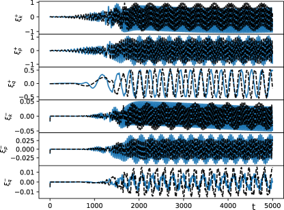
Figure 3: Comparison between exact or near resonances, with real parts of each eigenmode shown for each wave number as labeled on the left side of the figure. The solid line is the exact (i.e. $\Delta\omega\approx 2\times 10^{-15}$) resonance of $\mathbf{k}=\left(0,1.125\right)$ with $\mathbf{p}=\left(-0.5,-1.0632325265492\right)$ whereas the dashed line is the near resonance with $\mathbf{p}=\left(-0.5,-1.0\right)$ and $\Delta\omega\approx 0.01$. While some details change, the overall behavior, and saturation levels are actually very similar.

II.1.1 Is there a difference between exact and near resonances?

We first pick a primary wave-number $\mathbf{k}=\left(0,1.125\right)$ which is the linearly most unstable mode on a grid with $dk_{x}=dk_{y}=0.125$ for the $C=1.0$ case and consider the resonance manifold as shown in figure 2a in order to pick a second wave-number $\mathbf{p}=\left(-0.5,-1.0\right)$ as the point on the $k$-space grid that is closest to the resonance manifold. The third wave-number $\mathbf{q}$ is computed from $\mathbf{k}+\mathbf{p}+\mathbf{q}=0$. While a direct numerical simulation only has the wave-numbers on grid points, a three wave equation solver is not constrained to such a grid. We can instead compute $\mathbf{p}$ to be exactly on the resonance manifold -at least within some numerical precision- for example by choosing $\mathbf{p}=\left(-0.5,-1.0632325265492\right)$. Solving the three wave equations numerically, using these slightly different sets of wave-numbers, we find that having exact resonance or near resonance (i.e. $\Delta\omega\approx 2\times 10^{-15}$ vs. $\Delta\omega\approx 0.01$ ) does not make much difference in terms of time evolution (see figure ), while picking something like $\mathbf{p}=\left(-0.5,-1.5\right)$, which gives $\Delta\omega\approx 0.07$ (with $\omega_{k}\approx 0.1$ for comparison) gives a completely different time evolution, where one of the modes keeps growing linearly without being able to couple to the other two. We verified this for a bunch of different sets of wave numbers, and while there are some differences in detail, generally both exactly resonant or near resonant triads lead to saturation but non-resonant triads can not saturate, possibly due to lack of efficient interactions. The boundary between what can be considered a near resonant vs. non-resonant interaction can actually be defined using this criterion. In particular, it seems that the triads with one of the frequencies much smaller than the other two (i.e. $\omega_{q}\ll\omega_{p}\sim\omega_{k}$) tend to support larger overall $\Delta\omega$, and nonetheless reach saturation. However it is not clear whether these observations from a single triad continue to hold when many triads are interacting with each other.

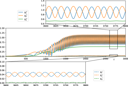
Figure 4: Time evolution of the amplitudes of the eigenmodes for $C=1$ case with $\mathbf{k}=\left(0,1.125\right)$ and $\mathbf{p}=\left(-0.5,-1.0\right)$. We have a “saturated” state with oscillating amplitudes. It seems that as $k$ and $p$ (the two unstable modes and the two larger legs of the triads) exchange energy, $q$ plays the role of the mediator.

II.2 Phase Evolution

Considering the (unwrapped) phase evolution of each of the modes of the near resonant triad with $\mathbf{k}=\left(0,1.125\right)$ and $\mathbf{p}=\left(-0.5,-1.0\right)$, we observe that while some amplitude evolution continues, the phases converge towards straight lines, implying more or less constant frequencies in the final stage. These nonlinear frequencies are substantially shifted with respect to the initial linear frequencies due to the effect of nonlinear terms. However it appears that the system remains in resonance as the sum of the final nonlinear frequencies remain very close to zero. In fact, it appears that the “near resonant” system evolves towards resonance as a result of these nonlinear corrections, since $\Delta\omega$ decreases from the beginning towards the end.

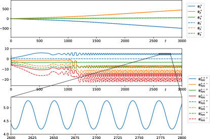
Figure 5: Time evolution of the phases $\varphi_{k}^{\pm}$ and their sums $\psi_{kpq}^{s_{p}s_{q}s_{k}}$ for $C=1$ case with $\mathbf{k}=\left(0,1.125\right)$ and $\mathbf{p}=\left(-0.5,-1.0\right)$. Saturation of the amplitudes as seen in figure 4 is accompanied by a nonlinear frequency shift as shown in the top plot and the saturation of the $\psi_{kpq}^{s_{p}s_{q}s_{k}}$’s as shown in the bottom plot. Note that $\psi_{kpq}^{s_{p}s_{q}s_{k}}=\text{const.}$ would correspond to phase locking.

Using (18) and (19) with the assumption that $\partial_{t}\chi_{k}^{\pm}\approx 0$ and $\partial_{t}\phi_{k}^{\pm}=-\omega_{k,\text{nl}}^{\pm}$ is a constant, we obtain the nonlinear frequency shift, i.e. $\delta\omega_{kr}^{\pm}=\omega_{k,\text{nl}}^{\pm}-\omega_{kr}^{\pm}$ as:

$$\delta\omega_{kr}^{\pm}=\text{sign}\left(\omega_{kr}\right)\sqrt{\frac{\left|N_{\xi k}^{\pm}\right|^{2}}{\left|\xi_{k}^{\pm}\right|^{2}}-\gamma_{k}^{\pm 2}}\;\text{,}$$ (26)

which can be computed given the final amplitudes and the nonlinear interaction coefficients (21). For example for the case above the smoothed saturated amplitudes are shown in the table:

	$k,+$	$p,+$	$q,+$	$k,-$	$p,-$	$q,-$
$\left|\xi\right|$	$0.89$	$0.93$	$0.52$	$0.041$	$0.040$	$0.0017$
$\omega_{r}$	$0.099$	$-0.088$	$-0.020$	$-0.099$	$0.088$	$0.020$
$\gamma$	$4.2\times 10^{-3}$	$3.1\times 10^{-3}$	$-1.8\times 10^{-4}$	$-1.8$	$-1.8$	$-4.8$
$\omega_{\text{nl}}$	$0.20$	$-0.19$	$-0.016$	$0.20$	$-0.19$	$-0.016$
$\delta\omega$	$0.11$	$-0.11$	$-0.075$	$-1.06$	$1.12$	$23.2$

Table 1: Saturated amplitudes, linear frequencies, linear growth rates, the final nonlinear frequencies and the $\delta\omega$’s that are computed from (26), rounded to two significant figures for the $C=1$ case with $\mathbf{k}=\left(0,1.125\right)$ and $\mathbf{p}=\left(-0.5,-1.0\right)$. Note that the basic assumption of (26) works only for linearly unstable modes, and for those $\delta\omega$ is not far from $\omega_{\text{nl}}-\omega_{r}$.

In order to elucidate dynamics of the phases in a triad, we define the sums of phases as a separate variable following Ref. 37:

$$\psi_{kpq}^{s_{k}s_{p}s_{q}}\equiv\varphi_{k}^{s_{k}}+\varphi_{p}^{s_{p}}+\varphi_{q}^{s_{q}}\;\text{.}$$ (27)

We observe that while the phases keep increasing in time, for a steady state, the phase differences should remain bounded. We can write the equations for the amplitudes as

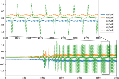
Figure 6: Time derivatives of the phases $\varphi_{k}^{\pm}$ for $C=1$ case with $\mathbf{k}=\left(0,1.125\right)$ and $\mathbf{p}=\left(-0.5,-1.0\right)$, corresponding to nonlinear frequencies. Notice that while $d\varphi_{q}^{-}/dt$ appears to oscillate wildly, since its amplitude $\chi_{q}^{-}$ is vanishingly small, as can be seen in figure 4, these oscillations are not important for the rest of the dynamics.

$$\partial_{t}\chi_{k}^{s_{k}} -\gamma_{k}^{s_{k}}\chi_{k}^{s_{k}}$$

$$= \sum_{\sigma_{p},\sigma_{q}}m_{kpq}^{s_{k}\sigma_{p}\sigma_{q}}\cos\left(\delta_{kpq}^{s_{k}\sigma_{p}\sigma_{q}}-\psi_{kpq}^{s_{k}\sigma_{p}\sigma_{q}}\right)\chi_{p}^{\sigma_{p}}\chi_{q}^{\sigma_{p}}$$ (28)

which contain the phases only through their sums (i.e. $\psi$ variables). We can also write an equation for the $\psi_{kpq}^{s_{k}s_{p}s_{q}}$ explicitly as:

$$\partial_{t}\psi_{kpq}^{s_{k}s_{p}s_{q}} +\text{$\left(\omega_{k}^{s_{k}}+\omega_{p}^{s_{p}}+\omega_{p}^{s_{q}}\right)$}$$

$$=\sum_{\sigma_{p},\sigma_{q}}m_{kpq}^{s_{k}\sigma_{p}\sigma_{q}}\sin\left(\delta_{kpq}^{s_{k}\sigma_{p}\sigma_{q}}-\psi_{kpq}^{s_{k}\sigma_{p}\sigma_{q}}\right)\frac{\chi_{p}^{\sigma_{p}}\chi_{q}^{\sigma_{q}}}{\chi_{k}^{s_{k}}}$$

$$+\sum_{\sigma_{q},\sigma_{k}}m_{pqk}^{s_{p}\sigma_{q}\sigma_{k}}\sin\left(\delta_{pqk}^{s_{p}\sigma_{q}\sigma_{k}}-\psi_{pqk}^{s_{p}\sigma_{q}\sigma_{k}}\right)\frac{\chi_{q}^{\sigma_{q}}\chi_{k}^{\sigma_{k}}}{\chi_{p}^{s_{p}}}$$

$$+\sum_{\sigma_{k},\sigma_{p}}m_{qkp}^{s_{q}\sigma_{k}\sigma_{p}}\sin\left(\delta_{qkp}^{s_{q}\sigma_{k}\sigma_{p}}-\psi_{qkp}^{s_{q}\sigma_{k}\sigma_{p}}\right)\frac{\chi_{k}^{\sigma_{k}}\chi_{p}^{\sigma_{p}}}{\chi_{q}^{s_{q}}}\;\text{.}$$ (29)

While the form of (29) looks terribly complicated (e.g. when we expand the sums we have $8$ equations, each of whom having $12$ terms on their right hand side) it is useful for insight into phase locking. For example by setting $\partial_{t}\psi_{kpq}^{s_{k}s_{p}s_{q}}=0$ in (29), and $\partial_{t}\chi_{k}^{s_{k}}=0$ in (28), we can obtain constant amplitude, phase locked solutions, if such solutions exist. Unfortunately, even the computation of this “fixed point” requires numerical analysis. We can also integrate (28-29) numerically, which gives exactly the same result as the system in terms of $\xi_{k}^{\pm}$.

III Interactions with Zonal Flows

When two non-zonal modes interact with a zonal one the evolution equations and the nonlinear interaction coefficients are different from non-zonal three wave interactions discussed in the previous section. Using the original variables $\Phi_{k}$ and $n_{k}$ as in (3-4), zonal and non-zonal modes interact with the same nonlinear interaction coefficients but different linear propagators. However, when we diagonalize the linear propagator, the nonlinear interaction coefficients for zonal and non-zonal modes differentiate.

In particular we have

$$M_{kpq}^{\phi s_{p}s_{q}}=-\frac{\hat{\mathbf{z}}\times\mathbf{p}\cdot\mathbf{q}\left(q^{2}-p^{2}\right)C^{2}}{4\Omega_{p}^{s_{p}*}\Omega_{q}^{s_{q}*}k^{2}p^{2}q^{2}}$$ (30)

$$M_{kpq}^{ns_{p}s_{q}}=\frac{\hat{\mathbf{z}}\times\mathbf{p}\cdot\mathbf{q}C}{4\Omega_{p}^{s_{p}*}\Omega_{q}^{s_{q}*}p^{2}q^{2}}\bigg{[} \left(B_{q}-i\Omega_{q}^{s_{q}*}\right)q^{2}$$

$$-\left(B_{p}-i\Omega_{p}^{s_{p}*}\right)p^{2}\bigg{]}$$ (31)

$$M_{kpq}^{s_{k}\phi s_{q}}=i\frac{\hat{\mathbf{z}}\times\mathbf{p}\cdot\mathbf{q}}{2\Omega_{q}^{s_{q}*}q^{2}}\bigg{[} \left(B_{q}-i\Omega_{q}^{s_{q}*}\right)q^{2}$$

$$-\left(B_{k}-i\Omega_{k}^{s_{k}}\right)\left(q^{2}-p^{2}\right)\bigg{]}$$ (32)

$$M_{kpq}^{s_{k}ns_{q}}=i\frac{\hat{\mathbf{z}}\times\mathbf{p}\cdot\mathbf{q}C}{2\Omega_{q}^{s_{q}*}q^{2}}$$ (33)

so that for three waves $k$, $p$ and $q$ with $q_{y}=0$, we can write:

$$\partial_{t}\overline{\Phi}_{q}+\nu_{ZF}\overline{\Phi}_{q}=\sum_{s_{k},s_{p}}M_{qkp}^{\phi s_{k}s_{p}}\xi_{k}^{s_{k}*}\xi_{p}^{s_{p}*}$$ (34)

$$\partial_{t}\overline{n}_{q}+D_{ZF}\overline{n}_{q}=\sum_{s_{k},s_{p}}M_{qkp}^{ns_{k}s_{p}}\xi_{k}^{s_{k}*}\xi_{p}^{s_{p}*}$$ (35)

$$\partial_{t}\xi_{k}^{s_{k}}+i\omega_{k}^{s_{k}}\xi_{k}^{s_{k}}=\sum_{s_{p}}M_{kpq}^{s_{k}s_{p}\phi}\xi_{p}^{s_{p}*}\Phi_{q}^{*}+M_{kpq}^{s_{k}s_{p}n}\xi_{p}^{s_{p}*}n_{q}^{*}$$ (36)

$$\partial_{t}\xi_{p}^{s_{p}}+i\omega_{p}^{s_{p}}\xi_{p}^{s_{p}}=\sum_{s_{p}}M_{pqk}^{s_{p}\phi s_{k}}\Phi_{q}^{*}\xi_{k}^{s_{k}*}+M_{pqk}^{s_{p}ns_{k}}n_{q}^{*}\xi_{k}^{s_{k}*}\;\text{.}$$ (37)

We can write these in the form (23-25) by letting $\xi_{q}^{+}=\Phi_{q}$ and $\xi_{q}^{-}=n_{q}$ and paying attention to the form of the interaction coefficient $M_{\xi kpq}^{s_{k}s_{p}s_{q}}$ when one of the legs is zonal.

In order to study the interactions between two modes with a zonal flow in the Hasegawa-Wakatani system numerically, we pick a primary wave-number $\mathbf{k}=\left(0,1.125\right)$ which is the linearly most unstable mode on a grid with $dk_{x}=dk_{y}=0.125$ for the $C=1.0$ case. We choose $\mathbf{p}=\left(-0.5,-1.125\right)$ so that $\mathbf{q}=\left(0.5,0\right)$ is a zonal wave number. The $6$ field variables are now $\xi_{k}^{\pm}$, $\xi_{p}^{\pm}$, $\Phi_{q}$ and $n_{q}$ whose evolutions are shown in figure 7 for the case $C=1$, $\nu_{Z}=D_{Z}=0$ and $\gamma_{k}\gtrsim\gamma_{p}>0$. In the final state, the system finds a fixed point characterized by constant nonlinear frequency shifts, constant amplitudes and constant $\psi_{kpq}$’s. However this kind of steady state solution seems to be exclusive to the single triad case.

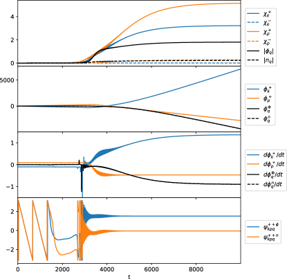
Figure 7: Time evolution of the three wave equations involving a zonal mode $q$, for the case $C=1$, $\nu_{Z}=D_{Z}=0$ and $\gamma_{k}\gtrsim\gamma_{p}>0$ with $k_{y}=1.125$ and $q=0.5$ [i.e. $\mathbf{k}=\left(0,k_{y}\right)$, $\mathbf{p}=\left(-q,-k_{y}\right)$ and $\mathbf{q}=\left(q,0\right)$]. The system reaches a steady state by introducing nonlinear frequencies in order to arrive at a state where the sums of phases $\psi_{kpq}$’s are constant. Note that it is $p$, which becomes the dominant mode in the final state and the existence of zonal flows does not lead to a complete suppression of turbulence. Instead the zonal flow acquires a constant nonlinear frequency.

III.1 Triad pairs

Because of the symmetry of the system, if we consider two wave-numbers $\mathbf{p}_{1}=-\mathbf{k}-\mathbf{q}$ and $\mathbf{p}_{2}=-\mathbf{k}+\mathbf{q}$ with $\mathbf{k}$ in $\hat{\mathbf{y}}$ and $\mathbf{q}$ in $\hat{\mathbf{x}}$ directions, we get two triads that are reflections of one another with respect to the axis defined by $\mathbf{k}$. Such a system involves four different wave-numbers connected with two different triads. Including the $p\rightleftarrows q$ transformation we have four triads as shown in figure 8. However as long as we use symmetric forms for the interaction coefficients, we can drop the two triads we obtain from the $p\rightleftarrows q$ transformation and count only two triads. Since the two triads of such a pair are reflections of one another, the nonlinear interaction coefficients differ only in sign while the complex frequencies are the same, and as there are two eigenmodes for each wave-number, we have $8$ equations. The equations for zonal modes can be written from (34-35) as:

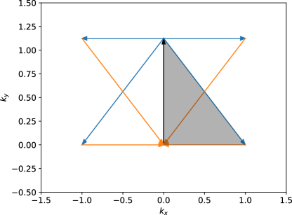
Figure 8: All the four triads involved in the interaction between the most unstable mode with $\mathbf{k}=k_{y}\hat{\mathbf{y}}$ with $k_{y}=1.125$ and a given zonal mode with $q=1.0$, obtained by reflection with respect to $\mathbf{k}$ and the exchange of $p$ and $q$ of the primary triad, which is shaded. The existence of the reflected triad is indeed important as it changes the qualitative behavior with respect to the single triad case.

$$\partial_{t}\Phi_{q}+\nu_{Z}\Phi_{q}=\sum_{s_{k},s_{p}}M_{qkp_{1}}^{\phi s_{k}s_{p}}\left(\xi_{k}^{s_{k}*}\xi_{p_{1}}^{s_{p_{1}}*}-\xi_{k}^{s_{k}}\xi_{p_{2}}^{s_{p_{2}}}\right)$$ (38)

$$\partial_{t}n_{q}+D_{Z}n_{q}=\sum_{s_{k},s_{p}}M_{qkp}^{ns_{k}s_{p}}\left(\xi_{k}^{s_{k}*}\xi_{p_{1}}^{s_{p}*}-\xi_{k}^{s_{k}}\xi_{p_{2}}^{s_{p}}\right)\;\text{,}$$ (39)

which is possible since $M_{\xi kp_{2}q}^{s_{k}s_{p}\left\{n,\phi\right\}}=-M_{\xi kp_{1}q}^{s_{k}s_{p}\left\{n,\phi\right\}}$ because $p_{2}^{2}=p_{1}^{2}$ and $p_{2y}=p_{1y}$ while $p_{2x}=-p_{2x}$. The equation for the primary mode, can be written as:

$$\partial_{t}\xi_{k}^{s_{k}}+i\omega_{k}^{s_{k}}\xi_{k}^{s_{k}} =\sum_{s_{p}}\bigg{[}M_{\xi kpq}^{s_{k}s_{p}\phi}\left(\Phi_{q}^{*}\xi_{p_{1}}^{s_{p}*}+\Phi_{q}\xi_{p_{2}}^{s_{p}*}\right)$$

$$+M_{\xi kpq}^{s_{k}s_{p}n}\left(n_{q}^{*}\xi_{p_{1}}^{s_{p}*}+n_{q}\xi_{p_{2}}^{s_{p}*}\right)\bigg{]}\;\text{,}$$ (40)

and the remaining two equations are the same as (37) but with different signs and conjugations:

$$\partial_{t}\xi_{p_{1}}^{s_{p}}+i\omega_{p_{1}}^{s_{p}}\xi_{p_{1}}^{s_{p}}=\sum_{s_{k}}\left(M_{\xi p_{1}kq}^{s_{p}s_{k}\phi}\Phi_{q}^{*}+M_{\xi p_{1}kq}^{s_{p}s_{k}n}n_{q}^{*}\right)\xi_{k}^{s_{k}*}$$ (41)

$$\partial_{t}\xi_{p_{2}}^{s_{p}}+i\omega_{p_{2}}^{s_{p}}\xi_{p_{2}}^{s_{p}}=-\sum_{s_{k}}\left(M_{\xi p_{1}kq}^{s_{p}s_{k}\phi}\Phi_{q}+M_{\xi p_{1}kq}^{s_{p}s_{k}n}n_{q}\right)\xi_{k}^{s_{k}*}$$ (42)

where $\omega_{p_{2}}^{s_{p}}=\omega_{p_{1}}^{s_{p}}$. Notice that this is also equivalent to one of the radial Fourier modes of a quasi-linear (e.g. zonostrophic) interaction, where for each field one would consider a single $p_{y}$ but the full spatial dependence in $x$.

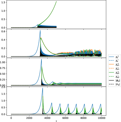
Figure 9: Evolution of a triad pair with the same parameters as figure 7, no zonal flow damping $\nu_{Z}=D_{Z}=0$ and $k_{y}=1.125$ [i.e. $\mathbf{k}=\left(0,k_{y}\right)$, $\mathbf{p}_{1}=\left(-q,-k_{y}\right)$, $\mathbf{p}_{2}=\left(q,-k_{y}\right)$ and $\mathbf{q}=\left(q,0\right)$] for four different values of $q=\left(1.0,1.5,2.0,4.0\right)$ from top to bottom for which the growth rates of the subdominant modes are $\gamma_{p}=\left(0.00099,-0.0016,-0.0042,-0.017\right)$ respectively. Note that apart from the second plot, which displays some chaotic behavior, the curves for $\xi_{p_{1}}^{+}$ and $\xi_{p_{2}}^{+}$ overlap almost exactly.

The results of the system (38-42) are shown in figure 9 for the $C=1$ case with $k_{y}=1.125$ [i.e. $\mathbf{k}=\left(0,k_{y}\right)$, $\mathbf{p}_{1}=\left(-q,-k_{y}\right)$, $\mathbf{p}_{2}=\left(q,-k_{y}\right)$ and $\mathbf{q}=\left(q,0\right)$] for $q=\left(1.0,1.5,2.0,4.0\right)$ from top to bottom respectively. For $q\leq k_{y}$ we have instability and $p$ keeps growing exponentially whereas for $q>k_{y}$ we get some sort of steady or limit cycle state. Performing a scan of $k_{y}$ and $q$ for this two triad system (keeping in mind that for $k_{y}>2$ we have no instability and therefore the pump mode decays) we observe that we can define a four wave interaction condition of the form $\omega_{kr}^{s_{k}}+\omega_{p1r}^{s_{p1}}+\omega_{p2r}^{s_{p2}}+\omega_{qr}^{s_{q}}=0$, which turns into $\Omega_{k}^{s_{k}}+2\Omega_{p}^{s_{p}}=0$ since $\omega_{qr}=0$ and $\omega_{p1r}=\omega_{p2r}=\omega_{pr}$. There seems to be $3$ distinct regions in figure X: for $q<1$, the $\xi_{p}^{+}$modes grow exponentially as in the top plot of figure 9, for the central region where $q\approx 1$, we have saturation and then somewhat chaotic evolution, and finally for $q\gg 1$, we observe limit cycle oscillations between $\xi_{k}^{+}$ and $\xi_{p}^{+}$ modes, mediated by zonal flows.

One is tempted to argue that since the $p$ with $p_{x}<p_{y}$ wins the competition to attract more energy, the cascade will proceed in this direction, and in the next step we can consider the interaction of this $\xi_{p}^{+}$ as the pump mode for the next triad etc. However, since each mode interacts with many triads simultaneously, the fact that $\xi_{p}^{+}$ wins the competition in the single triad (or one triad and its reflection) configuration does not really mean the energy will indeed go this way.

III.2 Triad Networks

In order to study the fate of the cascade, we need to consider multiple triads that are connected to one another. However as we add more zonal and non-zonal modes, it becomes quite complicated to keep track of all the interaction coefficients, conjugations etc. In order to simplify this task, we can divide the problem into two steps i) construction of a network of three body interactions and ii) computation of the evolution of the field variables on this network. For example for the above problem we need to consider a network of $N_{k}=4$ wave number nodes, coupled to $N_{t}=2$ triads, with $N_{f}=2$ fields in each node, with an interaction coefficient of the size $N_{f}\times N_{f}\times N_{f}$ for each connection. Since a network in Fourier space is made up of three body interactions, for each node, we can compute a list of interacting pairs and the interaction coefficients, so that we can write

$$\partial_{t}\xi_{\ell}^{i}+L_{\ell}^{ij}\xi_{\ell}^{j}=\frac{1}{2N}\sum_{\ell^{\prime},\ell^{\prime\prime}=\mathbf{i}_{\ell}}M_{\ell\ell^{\prime}\ell^{\prime\prime}}^{ijk}\left(\xi_{\ell^{\prime}}^{j}\right)^{c_{\ell^{\prime}}}\left(\xi_{\ell^{\prime\prime}}^{k}\right)^{c_{\ell^{\prime\prime}}}$$ (43)

where $\mathbf{i}_{\ell}$ is the list of precomputed interaction pairs for the node $\ell$. The indices $i$, $j$ and $k$ correspond to different fields (eigenmodes or $\Phi_{k}$ and $n_{k}$), the matrix $L_{\ell}^{ij}$ is the linear matrix in $k$ space (i.e. diagonal with the elements $i\omega_{\ell}^{\pm}$ for the eigenmodes), the $M_{\ell\ell^{\prime}\ell^{\prime\prime}}^{ijk}$ is the interaction coefficient for each interaction and $N$ is the number of independent wave number nodes so that when we reach the full grid, we have exactly the same interaction coefficients as the system formulated using discrete fast Fourier transforms (i.e. divided by $N_{x}\times N_{y}$). Finally if we write the triad interaction condition in the form $\mathbf{k}_{\ell}+\sigma_{\ell^{\prime}}\mathbf{k}_{\ell^{\prime}}+\sigma_{\ell^{\prime\prime}}\mathbf{k}_{\ell^{\prime\prime}}=0$ , where $\sigma$ are $\pm 1$, the $\left(\xi_{\ell^{\prime}}^{j}\right)^{c_{\ell^{\prime}}}$ are defined as:

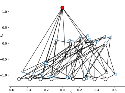
Figure 10: The structure of the network with a single $k_{y}$ with $k_{y}=1.125$ shown as a filled (red if in color) node. A reduced version with $q$ values that only go up to $0.5$ is shown for clarity. Notice that in this network while all of the $26$ triads involve one of the zonal modes, only $8$ of them involve the $q=0$ mode.

$$\left(\xi_{\ell^{\prime}}^{j}\right)^{c_{\ell^{\prime}}}=\begin{cases}\xi_{\ell^{\prime}}^{j}&\sigma_{\ell^{\prime}}=-1\\ \xi_{\ell^{\prime}}^{j*}&\sigma_{\ell^{\prime}}=+1\end{cases}$$

This is necessary unless we have the negative of each wave number vector as a separate node in the network.

Notice that when computing the nonlinear interaction coefficients for the eigenmodes, we would use (21) if all the nodes have nonzero $k_{y}$. In contrast we would use (30) and (31) if the receiving node (i.e. node $\ell$ ) is zonal or (32) and (33) if one of the interacting pairs (i.e. $\ell^{\prime}$ or $\ell^{\prime\prime}$) are zonal. Two or more zonal mode do not interact because of the geometric factor $\hat{\mathbf{z}}\times\mathbf{p}\cdot\mathbf{q}$, which appear in front of all the interaction coefficients.

Finally, if it makes sense to zero out some of the fields at a given wave-number (e.g. in eigenmode formulation, we may decide to throw away some damped modes), one may switch to a formulation where each node corresponds to a wave-number/field variable combination via $\left\{k_{x},k_{y},s_{k}\right\}\rightarrow\ell$. In this case, assuming that the linear matrix $L_{\ell}^{ij}$ in (43) diagonal takes the form:

$$\partial_{t}\xi_{\ell}+i\omega_{\ell}\xi_{\ell}=\frac{1}{N}\sum_{\ell^{\prime},\ell^{\prime\prime}=\mathbf{i}_{\ell}}M_{\ell\ell^{\prime}\ell^{\prime\prime}}\xi_{\ell^{\prime}}^{c_{\ell^{\prime}}}\xi_{\ell^{\prime\prime}}^{c_{\ell^{\prime\prime}}}$$ (44)

III.3 Order Parameters

The phases of wave-number nodes in Hasegawa-Wakatani turbulence evolve according to (19) or written explicitly as (22). This suggests that one can possibly define some kind of order parameter for this system. The usual definition of the Kuramoto order parameter can be written for the network formulation of (44) as:

$$z=re^{i\psi}=\frac{1}{N}\sum_{\ell}e^{i\varphi_{\ell}}$$ (45)

without explicitly distinguishing $+$ or $-$ modes. However this order parameter based on an unweighted sum is probably relevant only if all the oscillators were identical with all-to-all, unweighted couplings of the Kuramoto type. Instead we can use an amplitude filtered Kuramoto order parameter (i.e. the sum is computed only over the oscillators with an amplitude larger than a threshold), or define a weighted version of (45) as:

$$z=re^{i\psi}=\frac{\sum_{\ell}\chi_{\ell}e^{i\varphi_{\ell}}}{\sum_{\ell}\chi_{\ell}}$$ (46)

whose absolute value would tends towards $1$ if the relevant phases (i.e. those that have large amplitude) are the same. However note that the weighted order parameter tends towards $1$ also when one of the modes dominate over the others, while $\psi$ as defined in (46), can still be used as a mean phase.

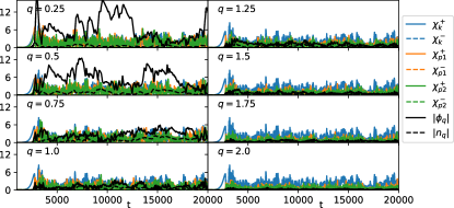
Figure 11: Time evolution for a number of triad pairs (as defined in section III.1) with different values of $q$ in the network of interacting triads for $C=1$ case with $\nu_{ZF}=D_{ZF}=10^{-3}$. A steady state turbulence level is observed, with elevated levels of zonal flows at large scales.

It would also make sense to look at the net effect on the nonlinear term on the phases instead. As discussed in Section I.2, since we can write:

$$\partial_{t}\varphi_{\ell}=-\omega_{\ell}+\frac{1}{N\chi_{\ell}}\text{Im}\left[\sum_{\ell^{\prime},\ell^{\prime\prime}=\mathbf{i}_{\ell}}M_{\ell\ell^{\prime}\ell^{\prime\prime}}\xi_{\ell^{\prime}}^{c_{\ell^{\prime}}}\xi_{\ell^{\prime\prime}}^{c_{\ell^{\prime\prime}}}e^{-i\varphi_{\ell}}\right]$$ (47)

for the evolution of the phase, we can define:

$$Z_{\ell}=R_{\ell}e^{i\psi_{\ell}}=\frac{1}{N\chi_{\ell}}\left(\sum_{\ell^{\prime},\ell^{\prime\prime}=\mathbf{i}_{\ell}}M_{\ell\ell^{\prime}\ell^{\prime\prime}}\xi_{\ell^{\prime}}^{c_{\ell^{\prime}}}\xi_{\ell^{\prime\prime}}^{c_{\ell^{\prime\prime}}}\right)$$ (48)

with $d_{\ell}$ being the number of interactions for the node $\ell$ (i.e. length of $\mathbf{i}_{\ell}$), as some kind of local order parameter for the node $\ell$, allowing us to write the phase equation as:

$$\partial_{t}\varphi_{\ell}=-\omega_{\ell}+R_{\ell}\sin\left(\psi_{\ell}-\varphi_{\ell}\right)\;\text{,}$$ (49)

which attracts the system towards $\varphi_{\ell}=\psi_{\ell}+2n\pi$.

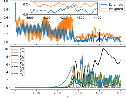
Figure 12: The top plot shows the order parameter $r$ defined in (45) or (46) as a function of time for a network with single $q$ and multiple $k_{y}$. The two definitions are in reasonable agreement apart from the peak around $t=2500$ for the weighted order parameter, which corresponds to the linear growth phase, where only a few modes around the most unstable mode dominate. This can be seen at the bottom plot where the amplitudes of a triad pair with $q=0.5$ and $k_{y}=1.125$ are shown. Around $t=2500$ the blue curve clearly dominates.

III.4 Specific network configurations

III.4.1 Network with a single $k_{y}$:

We consider a network of triad pairs as discussed in section III.1, with a single value of $k_{y}$ and $q$ values that go from $0.125$ to $4.0$ in steps of $0.125$. Notice that such a network has many different types of interactions as shown in figure 10, but all of those involve one of the zonal modes, which means that if we compute the inverse Fourier transform in the $x$ direction, the network can be seen to be equivalent to the single $k_{y}$, full-$x$, quasi-linear model [38, 39], since in both cases we have full spatial evolution but only nonlinear coupling is with the zonal flow.

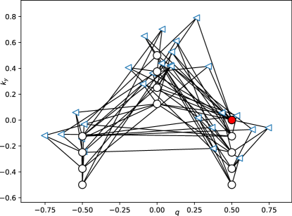
Figure 13: The structure of the network with a single $q=0.5$ zonal mode, shown as a filled (red if in color) node. A reduced version with $k_{y}$ values that only go up to $0.5$ is shown for clarity. Only $8$ of the full $26$ triads involve the zonal flow.

For the case $C=1$, without zonal flow damping (not shown) we observe that the zonal flows dominate and all the other modes decay to zero. This may well be what happens also in direct numerical simulations (DNS) eventually: what we observe in numerical simulations without zonal flow damping is a continual increase of zonal flows even for very long simulations.

In contrast, when we introduce zonal flow damping by letting $\nu_{ZF}=D_{ZF}=10^{-3}$, we get dynamics and $k$-spectra which look more like fully developed Hasegawa-Wakatani turbulence, as shown in figure 11, with high levels of zonal flows at large scales.

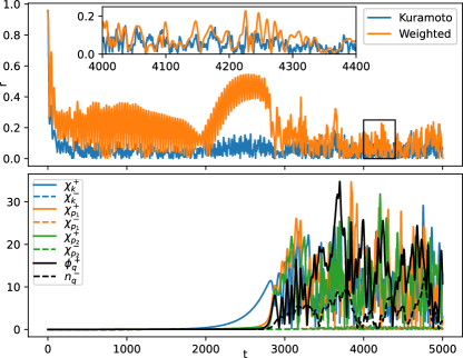
Figure 14: The top plot shows the order parameter $r$ defined in (45) or (46) as a function of time for a network with single $q$ and multiple $k_{y}$. The two definitions are in reasonable agreement apart from the peak around $t=2500$ for the weighted order parameter, which corresponds to the linear growth phase, where only a few modes around the most unstable mode dominate. This can be seen at the bottom plot where the amplitudes of a triad pair with $q=0.5$ and $k_{y}=1.125$ are shown. Around $t=2500$ the blue curve clearly dominates.

III.4.2 Network with a single $q$:

Here, we consider a network of triad pairs with a single $q$, and a grid of values of $k_{y}$ going from $0.125$ to $4.0$ in steps of $0.125$. A reduced version of such a network is shown in figure 13. Physically this network corresponds to the opposite case where we consider a single $q$ with the whole $y$ dynamics if we compute the inverse Fourier transform in $y$. Since it involves bunch of oscillators with different frequencies (as $\omega$ is mostly a function of $k_{y}$) that are coupled to each other and to a zonal mode that may play the role of a dominant mean field, it has the basic ingredients that may lead to synchronization.

Nonetheless numerical observations suggest that there is no obvious route to global synchronization in the three body network of interacting triads consisting of a zonal mode and drift waves of different $k_{y}$ either. The weighted order parameter shows a brief increase during the nonlinear saturation phase as the energy is transferred to the zonal flow, but otherwise remain close to zero, while the Kuramoto order parameter simply remains close to zero the whole time as can be seen in figure 14. Since we observed no qualitative difference between the runs with or without zonal flow damping for this case, we only show those with $\nu_{ZF}=D_{ZF}=10^{-3}$.

III.5 Direct numerical simulations

One can think of direct numerical simulation (DNS) on a regular rectangular grid as a “network” in Fourier space, in the sense that it consists of a collection of wave number nodes connected to each other through triadic interactions. In contrast to the networks that we considered that contain a single zonal mode, or a single $q=0$ mode, a regular rectangular grid has all the possible wave-numbers in a particular range, and it allows using more efficient methods for computing the convolution sums. In practice, the high resolution direct numerical simulations that we discuss here were performed with a standard pseudo-spectral solver (i.e. with periodic boundary conditions in both directions) using 2/3 rule for dealiasing and adaptive time stepping.

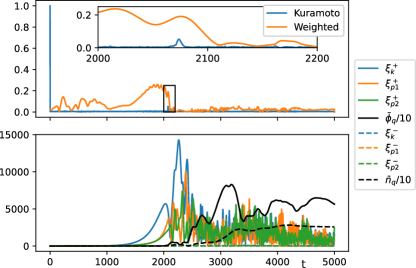
Figure 15: The top plot shows the order parameter $r$ defined in (45) or (46) as a function of time for a DNS. The bottom plot shows the amplitudes of a triad pair with $q=0.5$ and $k_{y}=1.125$ in order to compare with the earlier plots. The saturation levels for the amplitudes are different because of the normalization factor $N_{x}^{-1}N_{y}^{-1}$ in front of the nonlinear term implied in discrete Fourier transforms.

As with all the previous examples of single or multiple triads, or networks with a particular selection of nodes and triads, we use $C=1$, $\kappa=0.2$. Since we have a larger range of wave-numbers, we choose $\nu=D=10^{-4}$, with a box size of $L_{x}=L_{y}=16\pi$ and a padded resolution of $1024\times 1024$. The results show (see figures 15 and 16):

1. Initial linear growth followed by nonlinear saturation.

2. Formation and finally suppression of nonlinear of convective cells that transfer vorticity radially.

3. Consequent stratification of vorticity leading to a state dominated by zonal flows (as in figure 16).

4. Coherent nonlinear structures (e.g. vortices) that are advected by the zonal flows in regions of weak zonal shear, get sheared apart if they fall into a region of strong zonal shear.

Since the wave-like dynamics seems to be primarily in $y$ direction and reasonably localized in $x$, we can compute the Fourier transform in $y$ and plot phase of $\xi_{k_{y}}^{\pm}=\chi_{k_{y}}^{\pm}e^{i\phi_{k_{y}}^{\pm}}$ at each $x$, compute $\partial_{t}\phi_{k_{y}}^{\pm}\left(x,t\right)$ in order to compute the phase speeds (see figure 17). We can also compute an order parameter as a function of $x$ and $t$ from this data.

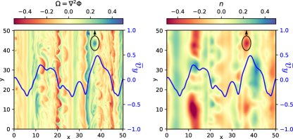
Figure 16: Snapshots of vorticity and density at t=5000 from DNS. The blue curve in both plots shows the zonal velocity whose values are given on the right hand axes. An example coherent vortex, that was moving upwards is encircled.

While it is clear from 15 that there is no global synchronization in direct numerical simulations, the plateau form of the phase velocity as a function of $k_{y}$ at the radii where it is positive for large scales, suggest that a process of phase locking similar to soliton formation in nonlinear Schrödinger equation, where nonlinearity would balance dispersion is at play for a range of $k_{y}$ values around the linearly unstable mode. While $\omega/k_{y}$ being the same across a range of $x$ and $k_{y}$ values is obviously very different from $\omega$ being the same. However if we note that the nonlinear dispersion relation takes the form $\omega\left(x,k_{y}\right)=\overline{v}_{\phi}\left(x\right)k_{y}$, at the lowest order we can see that the frequency in the frame moving with the zonal flow velocity becomes zero. This is roughly consistent with what we see in time evolution, where coherent structures like rotating vortices are advected by zonal flows. In order for such a detailed structure

IV Conclusion

A detailed analysis of triadic interactions formulated in terms natural frequencies reveals the complex nature of the dynamics of the phases and amplitudes in the Hasegawa Wakatani system. In particular, it is observed that a single resonant (or near resonant) triad, including a pump mode and two other modes, can saturate by adjusting the sums of phases of its legs ($\psi_{kpq}^{s_{k}s_{p}s_{q}}=\phi_{k}^{s_{k}}+\phi_{p}^{s_{p}}+\phi_{q}^{s_{q}}$) to be asymptotically constant, resulting in a set of nonlinearly shifted frequencies and constant amplitudes. When the interactions with zonal flows are considered, a similar saturation is possible for a single triad even without the condition of resonance. However this solution breaks down when we add the triad, which is the reflection of the original one with respect to the $y$ axis (or the wave-vector $\mathbf{k}$ vector). Instead we observe three different behavior for these triad pairs as a function of the radial wave number.

1. For smaller radial wave numbers, we find that the subdominant mode becomes the dominant one and grows exponentially. We call those unstable triads. They are associated with unstable subdominant modes.

2. For medium radial wave numbers, after an initial growth phase, the system saturates with a more or less chaotic evolution, where the energy goes back and forth between the modes. We call these saturated triads. They are associated with weakly unstable, or weakly damped subdominant modes.

3. For large radial wave numbers the system decays to a steady state solution after a number of limit cycle oscillations. In some cases, these limit cycle oscillations can continue until the end of the simulation time. We call these decaying triads (even though they don’t decay to zero but to a constant). They are associated with strongly damped subdominant modes.

In order to study the dynamics when those triads are connected to one another, we considered a network formulation where the wave numbers (or wave number eigenmode combinations) are considered as nodes, and each triad represents a three body interaction. It is shown while the zonal flow is almost never dominant in a single triad, when the whole triad network with a large number of triads is considered, the zonal modes become dominant almost in each triad. Thus, the system can reach a steady state where the zonal flow dominates as the other modes decay.

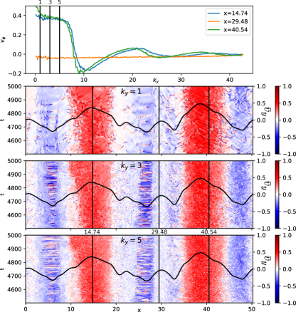
Figure 17: Profiles of phase velocity as a function of $k_{y}$, at three different values of $x$ (i.e. $14.74$, $29.48$ and $40.54$) averaged over $t=[4500,5000]$ shown at the top plot. The three plots that follow show the detailed time evolution (on the left $y$ axes) of phase velocity as a function of $x$ for three different values of $k_{y}$ (i.e. $1$, $3$ and $5$), together with the mean velocity profile shown for reference (on the right $y$ axes). The phase velocity is computed using $v_{\phi}=-\partial_{t}\phi_{k_{y}}^{+}\left(x,t\right)/k_{y}$. The $k_{y}$’s for which the time evolution is given and the $x$’s for which the phase velocities are shown are marked with horizontal lines in the corresponding figures.

In terms of triadic interactions, as the zonal flow becomes dominant, it plays the role of a collective mean field, in the sense that for each mode individual interactions with non-zonal modes start to become less important compared to the interaction with the zonal flow. This happens only when the number of triads is large enough so that the collective wins over the individual. It is interesting to note that this picture is qualitatively consistent with that of inhomogeneous wave-kinetic formulation, where the zonal flow is treated as a collective mean field, and the direct interaction between the modes are either dropped or modeled with a diffusion operator. This suggests that the wave-kinetic formulation may hold beyond its range of validity.

Playing with the range of radial wave-numbers of the network model, we observe that when the range includes only unstable triads [i.e. (i) above], or unstable and saturated triads [i.e. (i) and (ii) above] the network system remains unstable. It saturates only when we include a sufficient range of decaying triads, with subdominant modes with $\gamma_{p}^{+}<0$. This means that ’local coupling to damped modes’ (i.e. $\gamma_{p}^{-}$ modes even though $\gamma_{p}^{+}>0$) is not a real mechanism for turbulent saturation. However since the fact that $\gamma_{p}^{+}<0$ for those modes do not come directly from dissipation but rather the detailed form of the linear growth/damping whose form is determined by various parameters including dissipation, it is correct to argue that in contrast to the Kolmogorov picture where there is an injection scale, a dissipation scale and the inertial range in between, plasma turbulence can generate and dissipate energy in much closer scales, even though one may observe clear power law scalings.

One of the goals of the current paper was to study the effect of nonlinear synchronization of drift waves[40] on the turbulent cascade using a framework similar to the Kuramoto model[41], which has already been attempted using simple models in fusion plasmas[42, 43]. We hoped by considering a network of connected triads interacting with zonal flows we could setup a system that would tend toward synchronization through slight nonlinear modifications of the frequencies through their interactions with the zonal flow, playing the role of the control parameter. However due to particular form of the systematic dependency of the frequencies to the wave-numbers through the dispersion relation, such a system does not seem to tend towards synchronization. It should be checked whether or not the discretization resulting from boundary conditions, for example in cylindrical geometry change this picture drastically by impeding resonant interactions[44, 45] especially among large scale modes.

References

- Hasegawa and Wakatani [1983] A. Hasegawa and M. Wakatani, Pys. Rev. Lett 50, 682 (1983).
- Lesieur and Herring [1985] M. Lesieur and J. Herring, Journal of Fluid Mechanics 161, 77 (1985).
- Busse and Heikes [1980] F. H. Busse and K. E. Heikes, Science 208, 173 (1980).
- Currie and Tobias [2016] L. K. Currie and S. M. Tobias, Physics of Fluids 28, 017101 (2016).
- Hasegawa and Mima [1978] A. Hasegawa and K. Mima, Phys. Fluids 21, 87 (1978).
- Connaughton, Nazarenko, and Quinn [2015] C. Connaughton, S. Nazarenko, and B. Quinn, Physics Reports 604, 1 (2015).
- Diamond et al. [2005] P. H. Diamond, S.-I. Itoh, K. Itoh, and T. S. Hahm, PPCF 47, R35 (2005).
- Holland et al. [2007] C. Holland, G. R. Tynan, J. H. Y. A. James, D. Nishijima, M. Shimada, and N. Taheri, Plasma Physics and Controlled Fusion 49, A109 (2007).
- Pushkarev, Bos, and Nazarenko [2013] A. V. Pushkarev, W. J. T. Bos, and S. V. Nazarenko, Physics of Plasmas 20, 042304 (2013).
- Zhang and Krasheninnikov [2020] Y. Zhang and S. I. Krasheninnikov, Physics of Plasmas 27, 122303 (2020).
- Scott [1988] B. D. Scott, Journal of Computational Physics 78, 114 (1988).
- Koniges, Crotinger, and Diamond [1992] A. E. Koniges, J. A. Crotinger, and P. H. Diamond, Physics of Fluids B: Plasma Physics 4, 2785 (1992).
- Friedman and Carter [2015] B. Friedman and T. A. Carter, Physics of Plasmas 22, 012307 (2015).
- Sarto and Ghizzo [2017] D. D. Sarto and A. Ghizzo, Fluids 2 (2017), 10.3390/fluids2040065.
- Bos et al. [2010] W. Bos, B. Kadoch, S. Neffaa, and K. Schneider, Physica D: Nonlinear Phenomena 239, 1269 (2010), at the boundaries of nonlinear physics, fluid mechanics and turbulence: where do we stand? Special issue in celebration of the 60th birthday of K.R. Sreenivasan.
- Anderson and Hnat [2017] J. Anderson and B. Hnat, Physics of Plasmas 24, 062301 (2017).
- Gang et al. [1991] F. Y. Gang, P. H. Diamond, J. A. Crotinger, and A. E. Koniges, Physics of Fluids B: Plasma Physics (1989-1993) 3, 955 (1991).
- Hu, Krommes, and Bowman [1997] G. Hu, J. A. Krommes, and J. C. Bowman, Physics of Plasmas (1994-present) 4, 2116 (1997).
- Singh and Diamond [2021] R. Singh and P. H. Diamond, Plasma Physics and Controlled Fusion 63, 035015 (2021).
- Goumiri et al. [2013] I. R. Goumiri, C. W. Rowley, Z. Ma, D. A. Gates, J. A. Krommes, and J. B. Parker, Physics of Plasmas 20, 042501 (2013).
- Anderson et al. [2020] J. Anderson, E.-j. Kim, B. Hnat, and T. Rafiq, Physics of Plasmas 27, 022307 (2020).
- Heinonen and Diamond [2020] R. A. Heinonen and P. H. Diamond, Phys. Rev. E 101, 061201 (2020).
- Kasuya et al. [2007] N. Kasuya, M. Yagi, M. Azumi, K. Itoh, and S.-I. Itoh, Journal of the Physical Society of Japan 76, 044501 (2007).
- Vaezi et al. [2017] P. Vaezi, C. Holland, S. C. Thakur, and G. R. Tynan, Physics of Plasmas 24, 092310 (2017).
- Donnel et al. [2018] P. Donnel, P. Morel, C. Honoré, Ö. Gürcan, V. Pisarev, C. Metzger, and P. Hennequin, Physics of Plasmas 25, 062127 (2018).
- Smolyakov and Diamond [1999] A. I. Smolyakov and P. H. Diamond, Phys. Plasmas 6, 4410 (1999).
- Chen, Lin, and White [2000] L. Chen, Z. Lin, and R. White, Physics of Plasmas 7, 3129 (2000).
- Champeaux and Diamond [2001] S. Champeaux and P. Diamond, Physics Letters A 288, 214 (2001).
- Manz, Ramisch, and Stroth [2009] P. Manz, M. Ramisch, and U. Stroth, Phys. Rev. Lett. 103, 165004 (2009).
- Stroth, Manz, and Ramisch [2011] U. Stroth, P. Manz, and M. Ramisch, Plasma Physics and Controlled Fusion 53, 024006 (2011).
- Biglari, Diamond, and Terry [1990] H. Biglari, P. H. Diamond, and P. W. Terry, Phys. Fluids B 2, 1 (1990).
- Terry [2000] P. W. Terry, Rev. Mod. Phys. 72, 109 (2000).
- Malkov, Diamond, and Rosenbluth [2001] M. A. Malkov, P. H. Diamond, and M. N. Rosenbluth, Phys. Plasmas 8, 5073 (2001).
- Kim and Diamond [2003] E.-j. Kim and P. H. Diamond, Phys. Rev. Lett. 90, 185006 (2003).
- Guo and Diamond [2016] Z. B. Guo and P. H. Diamond, Phys. Rev. Lett. 117, 125002 (2016).
- Stoltzfus-Dueck, Scott, and Krommes [2013] T. Stoltzfus-Dueck, B. D. Scott, and J. A. Krommes, Physics of Plasmas 20, 082314 (2013).
- Bustamante and Kartashova [2009] M. D. Bustamante and E. Kartashova, Europhysics Letters 85, 34002 (2009).
- Bian et al. [2003] N. Bian, S. Benkadda, O. E. Garcia, J.-V. Paulsen, and X. Garbet, Physics of Plasmas 10, 1382 (2003).
- Sarazin et al. [2021] Y. Sarazin, G. Dif-Pradalier, X. Garbet, P. Ghendrih, A. Berger, C. Gillot, V. Grandgirard, K. Obrejan, R. Varennes, L. Vermare, and T. Cartier-Michaud, Plasma Physics and Controlled Fusion 63, 064007 (2021).
- Block et al. [2001] D. Block, A. Piel, C. Schröder, and T. Klinger, Phys. Rev. E 63, 056401 (2001).
- Kuramoto [1984] Y. Kuramoto, Chemical Oscillations, Waves, and Turbulence (Springer–Verlag, New York, 1984).
- Moradi, Anderson, and Gürcan [2015] S. Moradi, J. Anderson, and Ö. D. Gürcan, Physical Review E 92, 062930 (2015).
- Moradi, Teaca, and Anderson [2017] S. Moradi, B. Teaca, and J. Anderson, AIP Advances 7, 115213 (2017).
- Kartashova [1994] E. A. Kartashova, Phys. Rev. Lett. 72, 2013 (1994).
- Kartashova [2010] E. Kartashova, Nonlinear Resonance Analysis, by Elena Kartashova, Cambridge, UK: Cambridge University Press, 2010 1 (2010).