Energetic, tunable, highly-elliptically polarized higher harmonics generated by intense two-color counter rotating laser fields

Abstract

In this work, we demonstrate experimentally the efficient generation and tunability of energetic highly-elliptical high-harmonics in Ar gas, driven by intense two-color counter rotating laser electric fields. A bi-chromatic beam tailored by a MAZEL-TOV apparatus generates HHG, where the output spectrum of the highly elliptical HHG radiation can be tuned for a energy range of $\Delta$E$\HF$150 meV in the spectral range of $\HF$20 eV with energy per pulse E^XUV$\HF$400 nJ at the source. Furthermore we employ time-dependent density functional simulations to probe in-depth the dependence of the harmonic ellipticity and the strength of the isolated atto pulses on the driving field parameters and demonstrate the robustness of the HHG with the bichromatic field. We show how by properly tuning the central frequency of the second harmonic, the central frequency of the extreme ultraviolet (XUV) high harmonic radiation is continuously tuned. The demonstrated energy values largely exceed the output energy from many other laser driven attosecond sources reported so far and prove to be sufficient for inducing nonlinear processes in the atomic system. We envisage that such tunable energetic highly-elliptical HHG spectra can remove the facility restrictions from requirements of few-cycle driving pulses for isolated circular attosecond pulse generation.

I Introduction

Ultrafast chiral processes can be studied using high harmonic generation (HHG) (Baykusheva and Wörner, 2018; Ayuso et al., 2019; Cireasa et al., 2015; Heinrich et al., 2021; Neufeld and Cohen, 2018; Neufeld et al., 2019). HHG is an extreme nonlinear process, which depends on many parameters, such as the non-linear medium, the phase matching conditions, the peak intensity, the duration and the spectral phase of the driving pulse. By controlling these parameters it is possible to manipulate the spectral characteristics of the emitted extreme ultraviolet (XUV) radiation (Altucci et al., 1996; Chang et al., 1998; Lee et al., 2001; Winterfeldt et al., 2008). It has been demonstrated experimentally and theoretically that exploiting different mechanisms the harmonic HHG spectra can be influenced. Controlling parameters include the temporal chirp of the driving laser, the ionization-induced blue shift of the driver pulse in the generating medium (Froud et al., 2006; Altucci et al., 1996; Winterfeldt et al., 2008) and tuning the central wavelength of the driver using an optical parametric amplifier (Shan et al., 2002). HHG from linear polarized drivers produces harmonics with linear polarization and therefore severe limitations are imposed to the potential applications of an XUV HHG source Chordiya et al. (2023). In this context, the development of a tunable highly-elliptical XUV source adds an advanced tool. Such sources have recently emerged as a central topic of ultrafast science promising invaluable insights into chiroptical phenomena taking place on ultrashort time scales. Ultrashort circularly polarized pulses in the XUV domain have been generated at large-scale facilities, such as free-electron lasers(McNeil and Thompson, 2010; Higley et al., 2016; Lutman et al., 2016) and femto-sliced synchrotrons (Khan et al., 2006; Yamamoto et al., 2011; Čutić et al., 2011). In an effort to make such sources more broadly available, table-top sources based on high-harmonic generation (HHG) have also been developed (Kfir et al., 2015; Comby et al., 2020; Ferré et al., 2015; Hickstein et al., 2015; Vassakis et al., 2021; Comby et al., 2022).

The energy content of laser driven highly-elliptical or circularly polarized XUV radiation was limited to the pJ range per pulse (Kfir et al., 2015; Comby et al., 2020; Ferré et al., 2015; Hickstein et al., 2015) until recently when energy content in the nJ range were demonstrated in ref.(Vassakis et al., 2021). It is known that the recollision mechanism, which describes the HHG, entails that a stronger chiral response arises at the cost of a greatly suppressed high harmonic emission signal (Cireasa et al., 2015). Thus, the generation of energetic highly elliptical high harmonics is also a decisive step towards chiral-matter investigations.

In the present work, tunable energetic highly-elliptical HHG in the XUV regime is theoretically studied and experimentally demonstrated, exploiting two-color counter rotating electric fields under loose focusing geometry. The output spectrum of the highly elliptical HHG radiation can be tuned for an energy range of $\Delta$E$\HF$150 meV in the spectral range of $\HF$20 eV with energy per pulse E^XUV$\HF$400 nJ at the source.This is to our knowleeedge, the highest reported energy content per laser pulse in the laser-driven highly elliptical/circularly polarized XUV radiation.

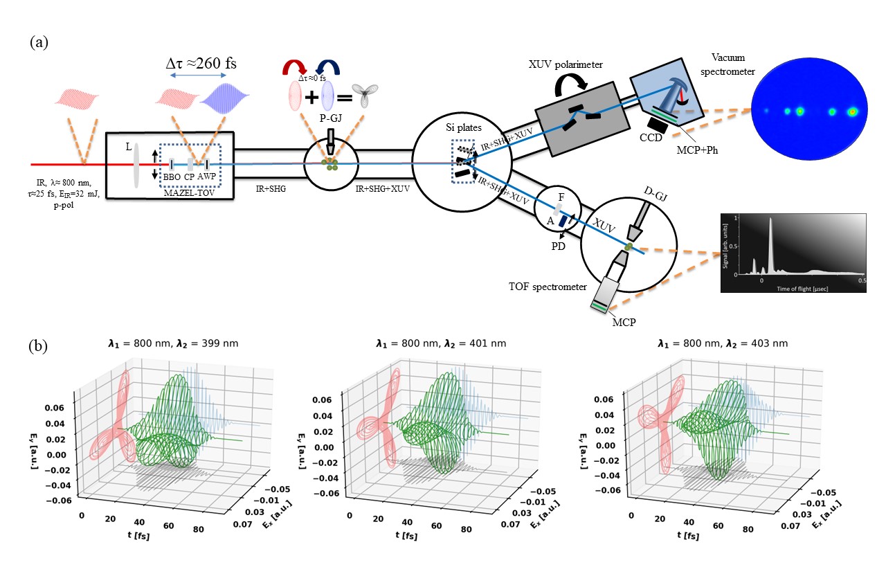
Figure 1: (a) Experimental apparatus for the generation of highly elliptical energetic tunable XUV radiation . A compact (15 cm long) MAZEL-TOV-like device is installed after a 3-m focal length lens (L). The device includes a BBO crystal, a calcite plate (CP) (both mounted independently on rotatable stages with high precision) and a rotatable super achromatic quarter waveplate(AWP). The two-color bi-circular field beam is focused into a pulsed gas jet filled with Ar (P-GJ). The generated XUV radiation is reflected towards the detection area by Si plates which consists of two branches. The first branch hosts a calibrated XUV photodiode (PD), a pulsed gas jet filled with Ar (D-GJ) and finally a $\mu$-metal shielded TOF spectrometer. The second branch hosts a rotating in-vacuum polarizer and consequently, the XUV radiation is diffracted by a spherical holohgraphic grating and detected by a microchannel-plate (MCP) detector coupled to a phosphor screen. (b) Calculated Bi-circular counter rotating electric field formed at the output of MAZEL-TOF-like device, based on our experimental parameters, with fundamental field having a central wavelength "$\lambda_{1}$" of 800 nm and three different second harmonic field wavelengths "$\lambda_{2}$", i.e., 399 (a), 401 (b), and 403 nm

II Adopted methodologies: experiments and simulations

For the experimental implementation, a compact MAch-ZEhnder-Less for Threefold Optical Virginia spiderwort-like (MAZEL-TOV-like (Kfir et al., 2016)) scheme is used to generate elliptically polarized HHG spectra. The technique is detailed in subsection 2.1, and schematically described in Fig. 1a. to In order to understand the spectral and temporal structure of the generated high-order harmonics our experimental characterizations and results are supported by theoretical simulations based on semi-classical approach, as elaborated in subsection 2.2 and time-dependent density functional theory in subsection 2.3, sub-cycle dynamics and crucial trends, identifying the factors in the estimated ellipticity of different harmonics.

II.1 Experimental Setup

The experiment was performed by exploiting the MW beamline of the Attosecond Science and Technology Laboratory (AST) at FORTH-IESL. The experiment utilizes a 10 Hz repetition rate Ti:Sapphire laser system delivering pulses with up to 400 mJ/pulse energy, $\tau_{L}$=25 fs duration and a carrier wavelength of 800 nm. The experimental set-up consists of three areas: the focusing and MAZEL-TOV-like (Kfir et al., 2016) device chamber, the harmonic generation chamber and the detection chambers (Fig.1). A laser beam of 3 cm outer diameter and energy of 32 mJ/pulse is passing through a 3 m focal-length lens with the MAZEL-TOV-like device positioned 1.25 meters downstream. The apparatus consists of a beta-phase barium borate crystal (BBO), a calcite plate and a super achromatic quarter waveplate. A fraction of the energy of the linear p-polarized fundamental pulse, is converted into a perpendicularly polarized (s-polarized) second harmonic field in a BBO (0.2 mm, cutting angle $29.20^{o}$ for type I phase matching). The conversion efficiency of the BBO crystal was maximized and it was found $\approx$ 30% at 403 nm. The run-out introduced by the BBO crystal for the SHG of 800 nm was determined to be 38.6 fs. It is noted that by placing the BBO after the focusing lens ensures that the wavefronts of the converging fundamental laser beam are reproduced into that of the second harmonic field. Therefore, the foci (placed close to a pulsed gas jet filled with Ar) of the $\omega$ and 2$\omega$ fields coincide along the propagation axis. Additionally, the beam passes through a calcite plate at almost normal incidence (AR coated, group velocity delay (GVD) compensation range 310-450 fs), which pre-compensates group delays introduced by the BBO crystal and the super achromatic quarter waveplate. The super achromatic waveplate converts the two-color linearly polarized pump into a bi-circular field, consisting of the fundamental field and its second harmonic, accumulating at the same time a group delay difference of ∼253 fs between the ∼400 nm and 800 nm central wavelengths. Assuming Gaussian optics, the intensity at the focus for the two components of the bi-circular polarized field is estimated to be $I_{\omega}$$\approx$$I_{2\omega}$$\approx$ 1x10¹⁴ W/cm². After the jet, the produced XUV co-propagates with the bi-circular driving fields towards a pair of Si plates, which are placed at 75^o reducing the p-polarization component of the fundamental and the second harmonic radiation while reflecting the harmonics (Takahashi et al., 2004) towards the detection area. The detection area conctinst of two branches. In the first branch which is placed directly after the first Si plate, a pair of 5 mm diameter apertures were placed in order to block the outer part of the $\omega$ and 2$\omega$ beams, while letting essentially the entire XUV through. A 150 nm thick Sn filter is attached to the second aperture, not only for the spectral selection of the XUV radiation, but also to eliminate the residual bicircular field. A calibrated XUV photodiode (XUV PD) can be introduced into the beam path in order to measure the XUV pulse energy. The transmitted beam enters the detection chamber, where the spectral characterization of the XUV radiation takes place. The characterization is achieved by recording the products of the interaction between the XUV beam and the Ar atoms. The electrons produced by the interaction of Ar atoms with the unfocused XUV radiation were detected by a $\mu$-metal shielded time-of-flight (TOF) spectrometer. The spectral intensity distribution of the XUV radiation is obtained by measuring the single-photon ionization photo-electron (PE) spectra induced by the XUV radiation with photon energy higher than the $I_{p}$ of Ar ($I_{pAr}$=15.76 eV). In the second branch and after the Si plate, a rotating in-vacuum polarizer is installed and consequently, the XUV radiation is diffracted by a spherical holographic grating and detected by a microchannel-plate detector (MCP) coupled with a phosphor screen.

II.2 Simulations

II.2.1 Semi-classical approach

In order to have an intuitive picture of the HHG by two color bi-circular polarized fields, we performed calculations based on the semicalssical approach where the theoretical framework and detailed analysis can be found elsewhere (Milosevic et al., 2000). In our supplementary material IV.4, we present an abbreviated analysis which is based on Strong Field Approximation (SFA)(Lewenstein et al., 1994) adapted in the case of these electric fields.

Within this model, the radiation at orders 3n$\pm 1$ (with n=1,2,3,…), emitted from a single atom exposed to a intense bi-chromatic driving electric field E(t) with the associated vector potential A(t) = − $\int\mathbf{E}(t)dt$ can be fully characterized by the Fourier transform of the time-dependent dipole moment. Details of this analysis can be found elsewhere (Nayak et al., 2019).

II.2.2 Time dependent density functional formalism

The time-dependent electron dynamics in Argon under the influence of bi-chromatic counter rotating (BCCR) laser fields are investigated based on ab-initio calculation within time dependent density functional theory (TDDFT) approach (Runge and Gross, 1984) in the real-time and real-space grids as implemented in the octopus computational package (Andrade et al., 2012, 2015). Thus, a more detailed and a more complete picture of these dynamics are presented.

The driving laser fields, as described in terms of an electric field, are polarized in the x-y plane and dipole approximation is considered. In addition, the contributions from magnetic component of the electromagnetic field and any other relativistic terms, such as spin-orbit coupling are neglected. The combined electric field is a superposition of two counter rotating laser fields, and is given as in 1.

$$\begin{split}E(t)=\sum_{i=1,2}E_{i}&\cos{\bigg{(}\frac{(t-\tau_{\omega 1})}{\tau_{\omega i}}\bigg{)}^{2}}\Bigg{[}\cos{\bigg{(}\omega_{i}(t-\tau_{\omega 1})\bigg{)}}\boldsymbol{e_{x}}+\\ &a_{i}\sin{\bigg{(}\omega_{i}(t-\tau_{\omega 1})\bigg{)}}\boldsymbol{e_{y}}\Bigg{]}\end{split}$$ (1)

where $e_{x}$ and $e_{y}$ are the two mutually perpendicular unit vectors. We considered two counter rotating fields of $a_{1}$ = $-a_{2}\leavevmode\nobreak\ =\leavevmode\nobreak\ 1$ with $E_{1}\leavevmode\nobreak\ =\leavevmode\nobreak\ E_{2}\leavevmode\nobreak\ =E_{0}$. The peak laser intensity is expressed in terms of field strength $E_{0}:I=E_{0}^{2}I_{a}$, where $I_{a}=3.51\times 10^{16}\leavevmode\nobreak\ W/cm^{2}$ is the atomic intensity unit. The peak intensity is $I=1\times 10^{14}\leavevmode\nobreak\ W/cm^{2}$. $\cos{\bigg{(}\frac{(t-\tau_{\omega 1})}{\tau_{\omega i}}\bigg{)}^{2}}$ denotes the envelope of the pulse, where $\tau_{\omega 1}$ is the total duration of the fundamental pulse, that may be defined in terms of full width at half maximum of intensity (FWHM), $\tau_{p}:\tau_{\omega 1}=\tau_{p}/(2\arccos{(2^{-1/4})})$, where $\tau_{p}=25$ fs. $\tau_{\omega 2}$ is the pulse duration of the second harmonic field, which is defined as $\tau_{\omega 2}=\tau_{\omega 1}/\sqrt{2}$. A central wavelength $\lambda_{1}=800$ nm is used for the fundamental field and four different wavelengths are used for the second harmonic field, which are $\lambda_{2}=399,\leavevmode\nobreak\ \text{or}\leavevmode\nobreak\ 400,\leavevmode\nobreak\ \text{or}\leavevmode\nobreak\ 401,\leavevmode\nobreak\ \text{or}\leavevmode\nobreak\ 403$ nm.

The initial states are obtained from self-consistent solutions of wave functions at the density functional theory (DFT) level. Later, those states are propagated by using the approximated enforced time-resolved symmetry (AETRS) method, with $\Delta t\leavevmode\nobreak\ =\leavevmode\nobreak\ 0.3$ a.u. time-steps. Rest of the TDDFT input parameters are presented in the supplementary material (IV.3). The harmonic spectral properties are calculated from the resulting dipole acceleration signal, which has components that are both parallel and perpendicular to the laser polarization. The harmonic spectrum $HHG(\omega)$ is obtained from the Fourier transformation of the time-dependent dipole acceleration a(t) and can be written as (Chu and Chu, 2001; Burnett et al., 1992),

$$HHG(\omega)=\bigg{|}\mathcal{FT}\bigg{(}\int_{-\infty}^{\infty}{a(t)\leavevmode\nobreak\ dt}\bigg{)}\bigg{|}^{2},$$ (2)

where, $\mathcal{FT}$ is the Fourier transform.

Three of the different bichromatic circularly polarized field variations having coplanar counter-rotating components, that are used in both experiment and simulations in our work, are shown in Fig. 1(b).

III Results and analysis

III.1 Highly-elliptical XUV radiation spectral characteristics

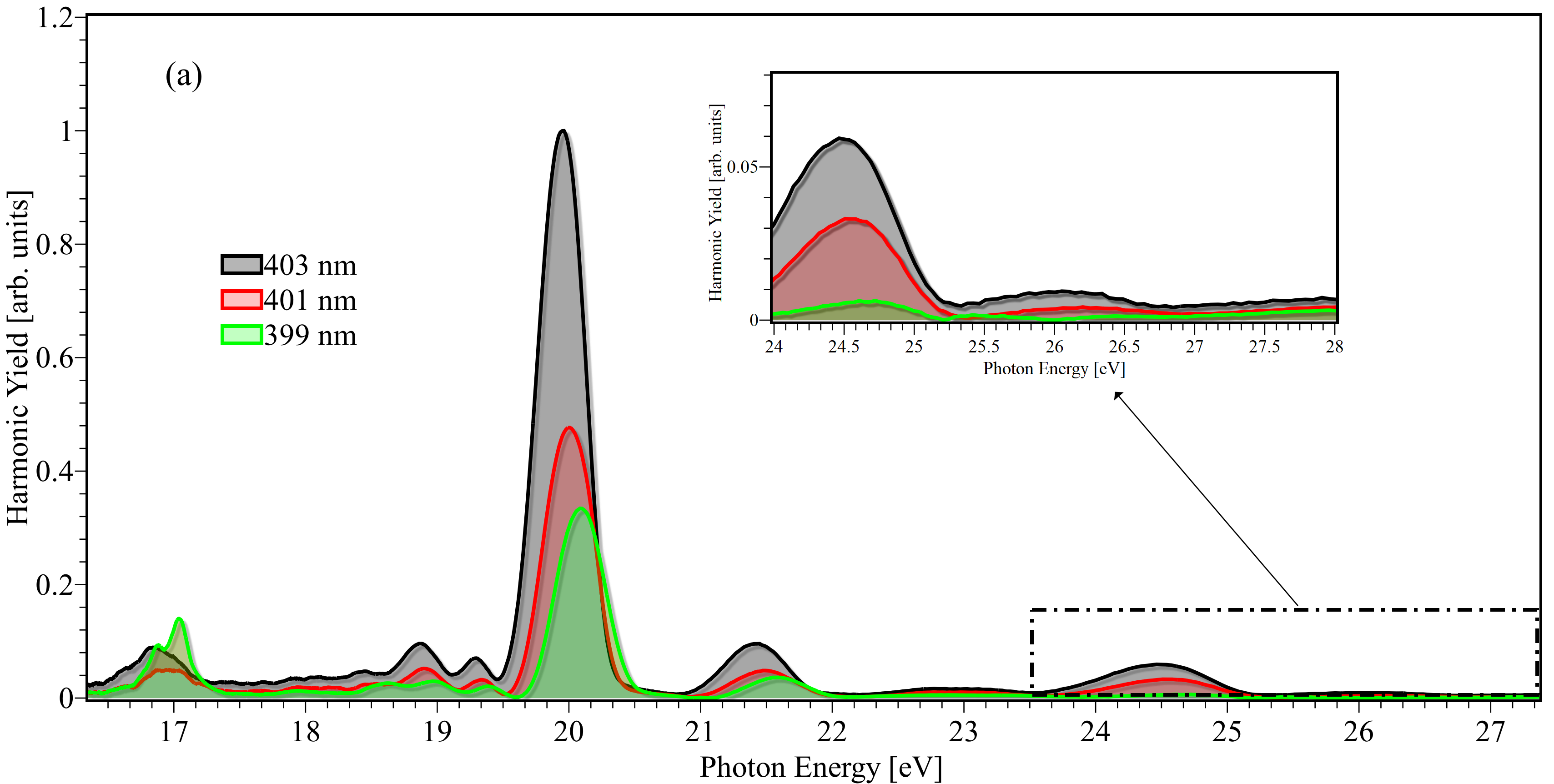
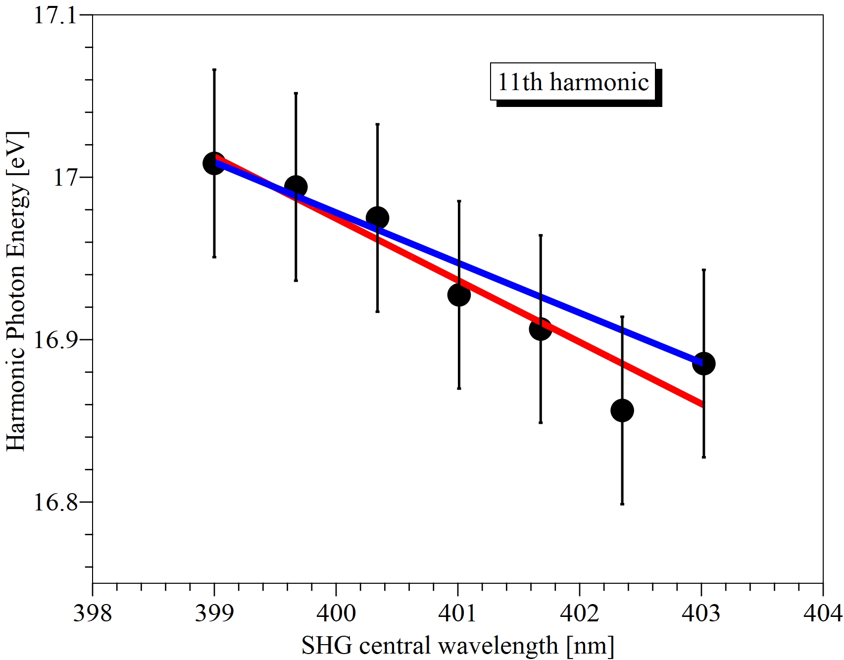
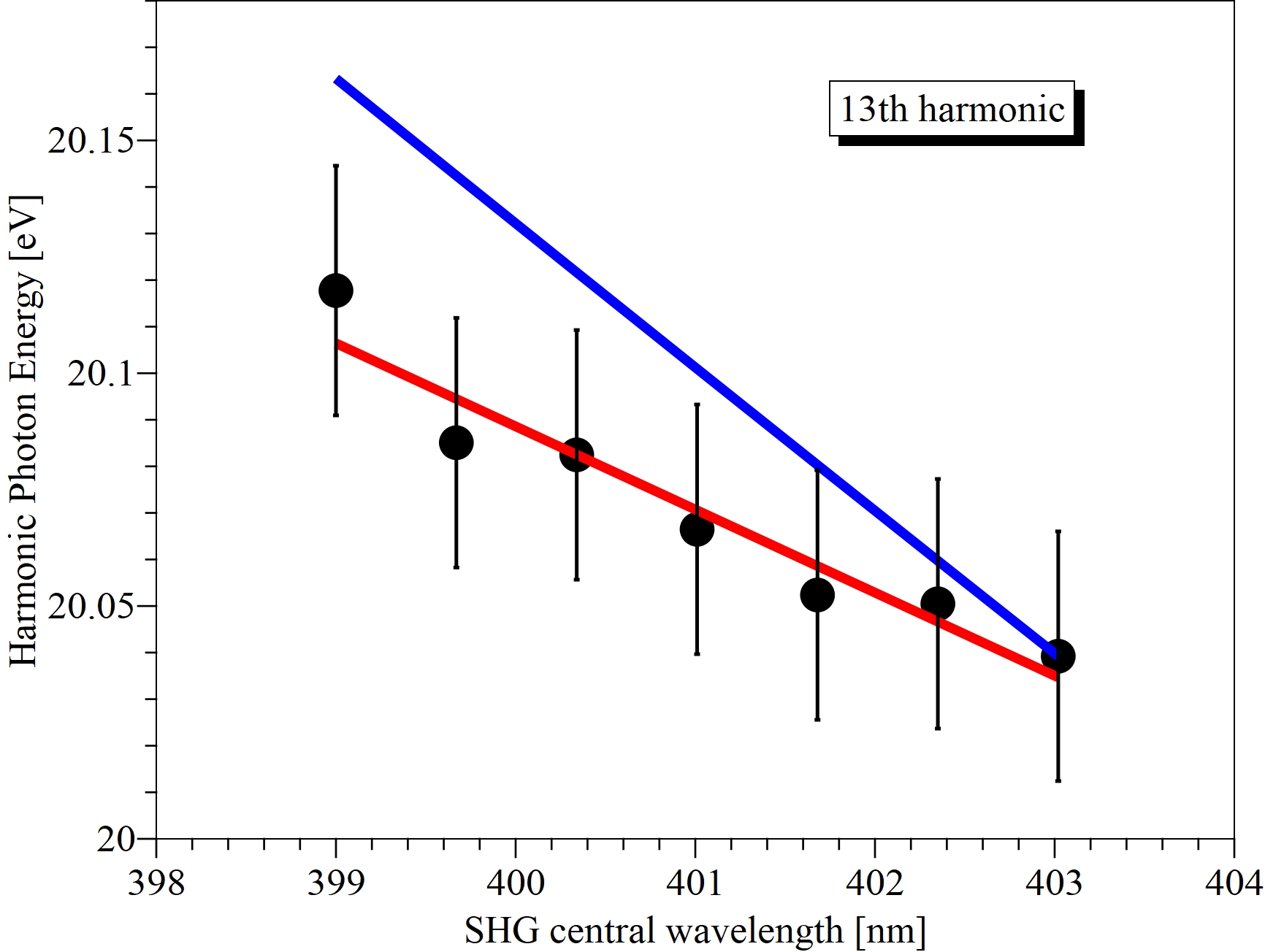
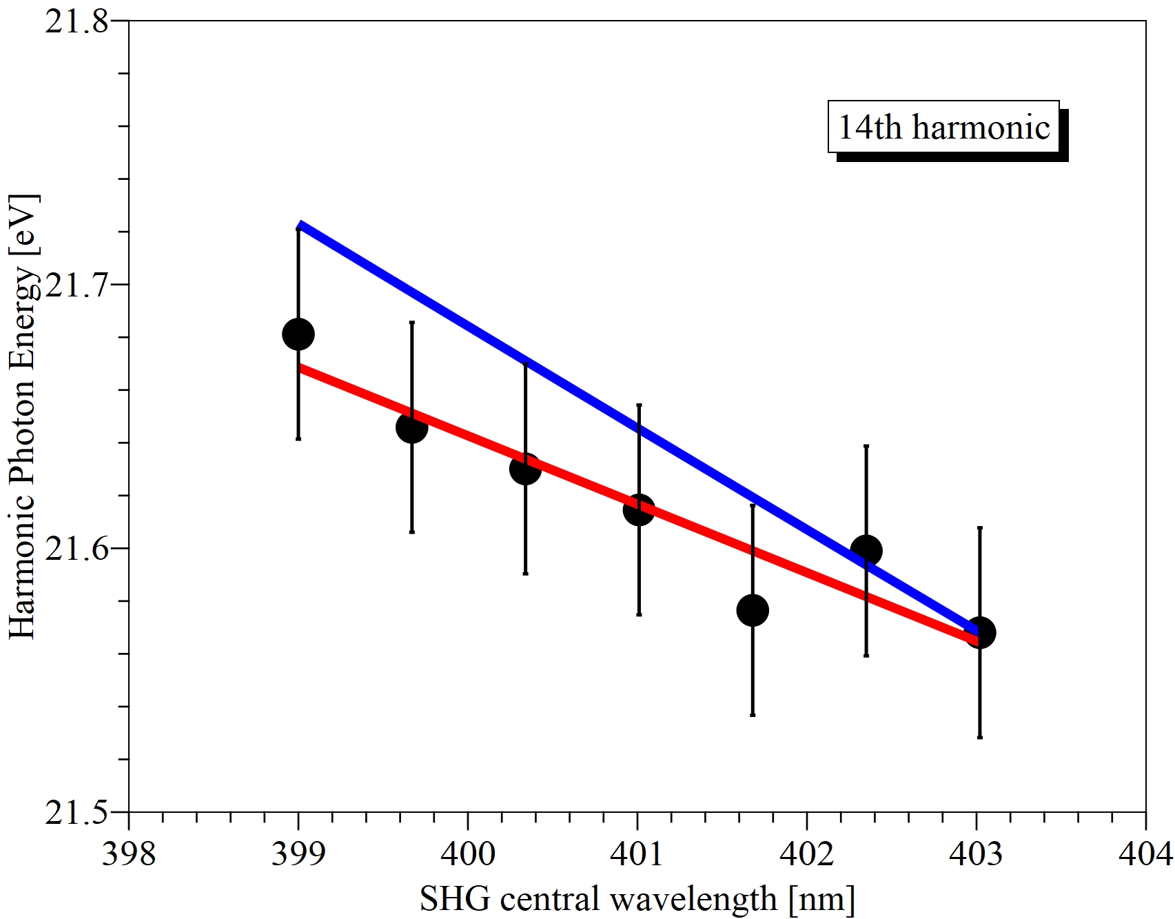
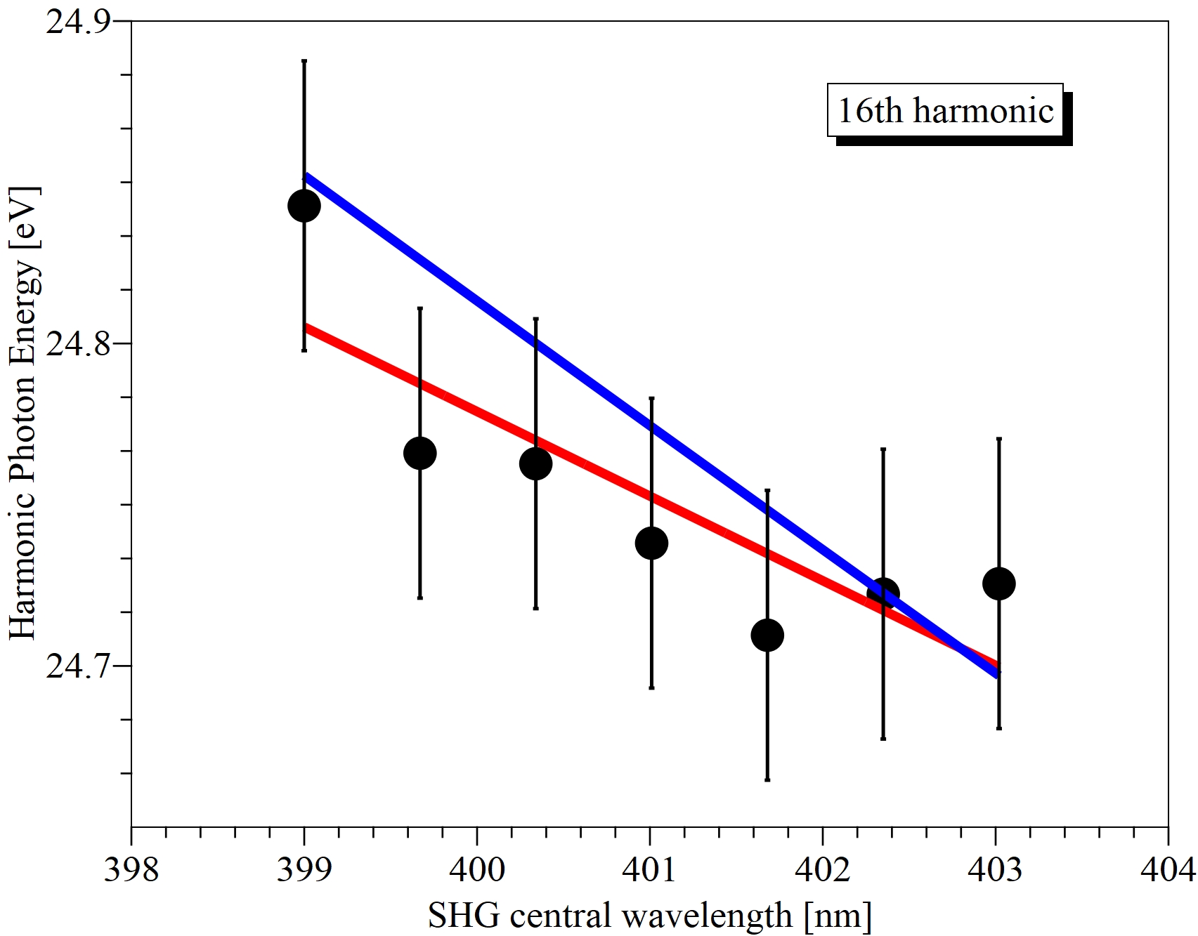
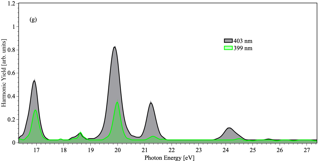
Figure 2: (a) Characteristic highly-elliptical HHG spectra for three different values of central SHG wavelength. The maximum energy shift observed is in the order of $\Delta$E$\HF$150 meV. (b),(c),(d),(e) Complementary analysis of the detectable harmonics (11^th,13^th,14^th and 16^th). An linear dependence of central HHG energy on the central wavelength of the SHG is observed. The blue line depicts the same dependence calculated from the energy conservation of the annihilated driver photons and the emitted XUV photon. Figure 2(g) presents highly-elliptical HHG spectra obtained by the vacuum spectrometer.

For the spectral characterization of the highly-elliptical XUV radiation different PE spectra were recorded as a function of the angle $\Delta$$\theta$ of the BBO crystal installed in the MAZEL-TOV-like device. Characteristic highly-elliptical HHG spectra are presented in Fig.2(a) for three different positions of $\Delta$$\theta$. An energy shift is clearly observed towards higher photon energies when the the angle ($\Delta$$\theta$) between the propagation axis of the IR driving field and the BBO crystal is increased. Additionally, in Fig.2(b),(c),(d),(e) complementary measurements of the detectable harmonics by the TOF spectrometer are presented. Finally, Fig. 2(g) presents highly-elliptical HHG spectra obtained by the vacuum spectrometer for reason of completeness. It is revealed that central HHG energy indicating almost linear dependence on the central wavelength of the SHG. The maximum energy shift observed is in the order of $\Delta$E$\HF$150meV. The observed blue shift can be attributed to the energy conservation of the HHG process by two color BCCR electric fields. From energy conservation, the harmonic frequencies generated by these fields is given as

$$\varOmega_{(n_{1},n_{2})}=n_{1}\cdot\omega+n_{2}\cdot\beta\omega$$ (3)

where, $n_{1}$ and $n_{2}$ are integer numbers that are associated with the number of photons involved in the process of HHG at angular frequencies $\omega$ and $\beta\omega$, respectively. On the other hand, parity and spin angular momentum conservation requires that $\varDelta n=n_{1}-n_{2}$=$\pm 1$. Therefore, in the case of 13^th harmonic and $1.985\leq\beta\leq 2.005$ (which reflects our experimental conditions), the unique pair ($n_{1},n_{2}$) associated with this harmonic is equal to (5,4). It becomes evident that a linear dependence of the generated harmonic photon energy is expected as a function of the parameter $\beta$ (as confirmed in Table 1).

In Fig.2(b),(c),(d),(e), is depicted with the blue line this dependence calculated from the energy conservation of the annihilated driver photons and the emitted XUV photons (Table 1)(Fleischer et al., 2014)

harmonic	(n1,n2)	$\Delta E/\Delta\lambda$ [eV/nm]
11th	(3,4)	-0,03086
13th	(5,4)	-0,03086
14th	(4,5)	-0,03858
16th	(6,5)	-0,03858
17th	(5,6)	-0,04656

Table 1: The slope $\Delta E/\Delta\lambda$ [eV/nm] respect to each harmonic order. For each harmonic order, the corresponding channel is also displayed, where n₁ is the number of photons of the fundamental field and n₂ is the number of photons of the second harmonic field.

From another perspective, this characteristic blue shift can be interpreted in the framework of Strong Field Approximation (SFA)(Lewenstein et al., 1994; Milosevic et al., 2000). The active electron acquires different complex phase in the continuum for each central SHG wavelength. This leads to constructive interference at different spectral positions inside the highly-elliptical HHG spectrum resulting to the observed blue shift in the energy domain.

III.2 Polarimetric investigation

The emitted harmonic radiation after the reflection of a Si plate is sent through a rotating in-vacuum polarizer, which consists of two UV protected silver(Ag)-coated and one UV protected aluminum-coated(Al) mirrors mounted on a common plate. The angle of incidence on each mirror is $75^{o}(Ag)$-$60^{o}(Al)$-$75^{o}(Ag)$ . Finally, the harmonic radiation is diffracted using a spherical holographic grating (platinum coated, 2400 G/mm) and detected by a multichannel-plate detector (MCP) coupled to a phosphor screen. The contrast of the rotating in-vacuum polarizer, was extracted by polarimetric measurements of the linear p-polarized XUV radiation (MAZEL-TOV-like device out of the beam line) which is presented in Fig. 3(a) and it was found to be R = 2.2 $\pm$ 0.1 by fitting the imperfect polarizer equation 18 (For the mathematical extraction of the imperfect polarizer equation see Section IV.2) . Polarimetric measurements were performed for the 10^th, 11^th, 13^th, 14^th harmonics as a function of the angle $\Delta$$\theta$. Therefore, polarization scans were acquired during which the polarizer was rotated between 0° and 360° in step of $\sim$8° and averaging of 40 pulses per step.

From these scans the ellipticity of the high harmonics as a function of the BBO angle was derived. The measurement of the state of polarization of the HHG spectra confirmed highly-elliptical polarization reaching ellipticities up to $\sim 70$% at $\sim$22 eV as it is presented in Fig. 4(a). No dependence on the central wavelength of the SHGwas found. Briefly, the polarization state of these highly elliptical harmonics was extracted by fitting the imperfect polarizer equation (18 of the Supplementary Material) on the raw data of the polarization scans keeping as only known parameter the contrast of the polarizer R = 2.2 $\pm$ 0.1. In the present configuration used for the characterization of the harmonic ellipticity includes the Si plate which reflects highly elliptical harmonic emission to the XUV polarimeter. This optical component provides marginally different reflectivity for the s and p polarization component of the XUV radiation affecting also the measured ellipticity of the HHG radiation. By calculating the reflectivity of the Si plate for the two polarization orientations by using the corresponding Fresnel equations using the refractive indexes taken from Palik et al.(Palik, 1997) and for each harmonic component the values of ellipticity at the source can be estimated. Therefore, ellipticities up to $\sim 85$% at $\sim$22 eV were found as it is shown in Fig. 4(b). These ellipticity values in conjuction with the high energy content of the XUV pulses, reveal a source adequate for in applications like control and imaging of ultrafast magnetism in magnetic materials (Kfir et al., 2017; Jilili et al., 2023; Siegrist et al., 2019), in ultrafast chiral matter investigations (Ferré et al., 2015) and also in the investigation of circular dichroism in atomic systems (Hofbrucker et al., 2018; Lambropoulos, 1972; Mayer et al., 2022) where intense highly-elliptical/cicrcularly polarized XUV radiation is necessary for inducing nonlinear processes(Lambropoulos, 1972).

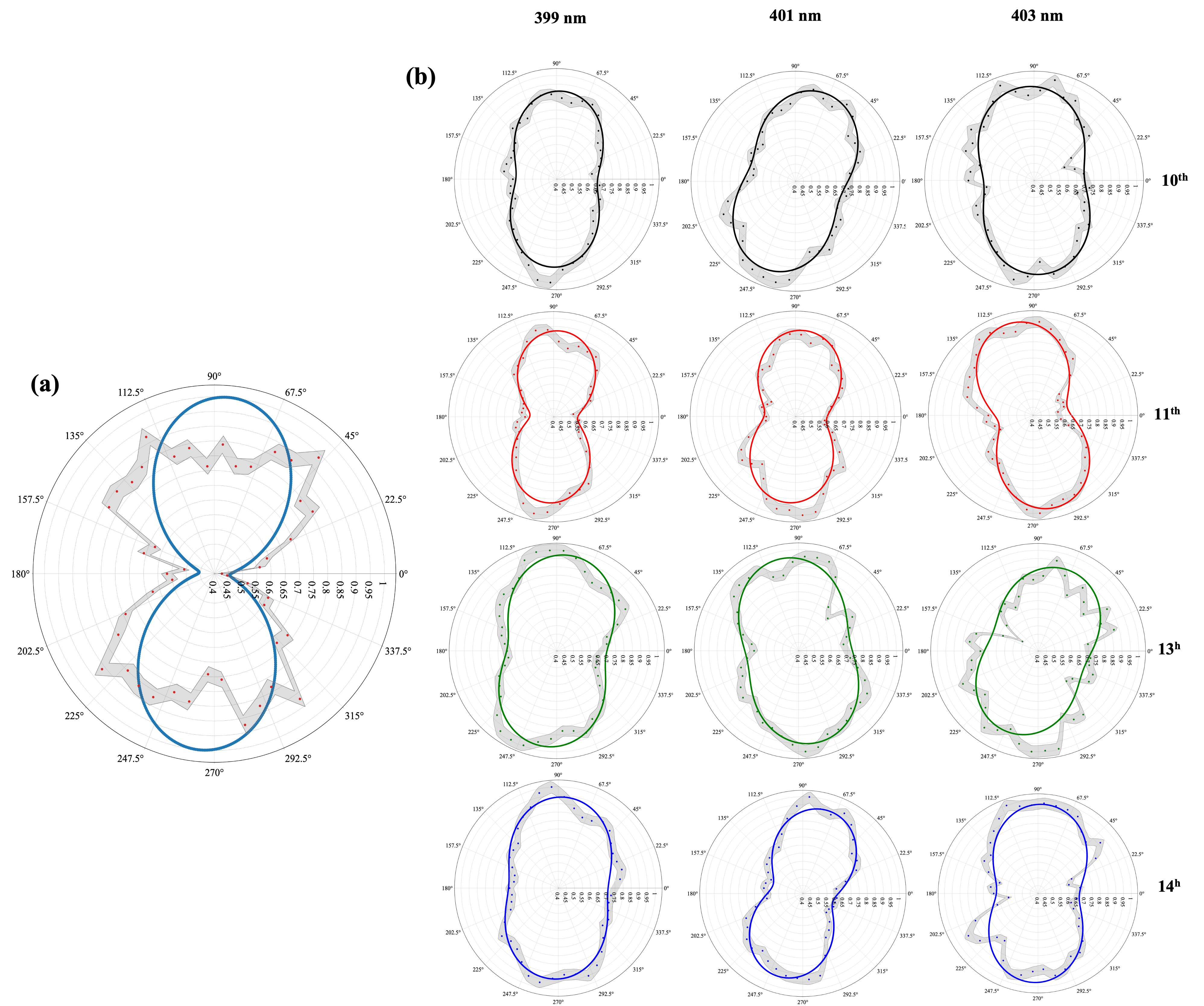
Figure 3: (a) Characteristic polarimetric measurment for the 11^th harmonic of the linear polarized driver. (b) Polarization scan for the 10^th, 11^th, 13^th, 14^th harmonics using for three different values of the BBO turning angle $\Delta$$\vartheta$ with respect to the propagation axis of the 25-fs IR laser pulse of the driver and thus different phase matching SHG central wavlelengths.

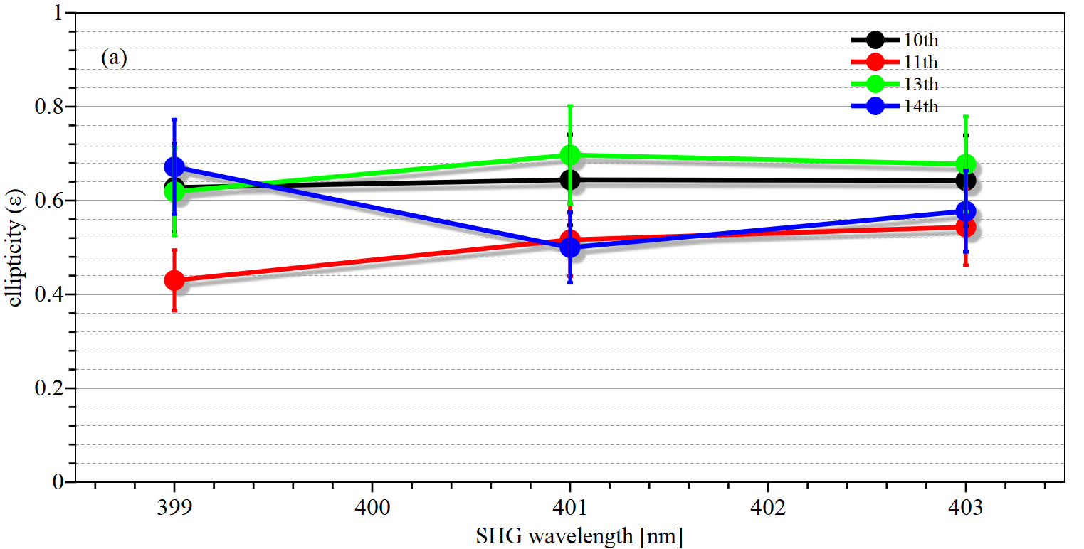
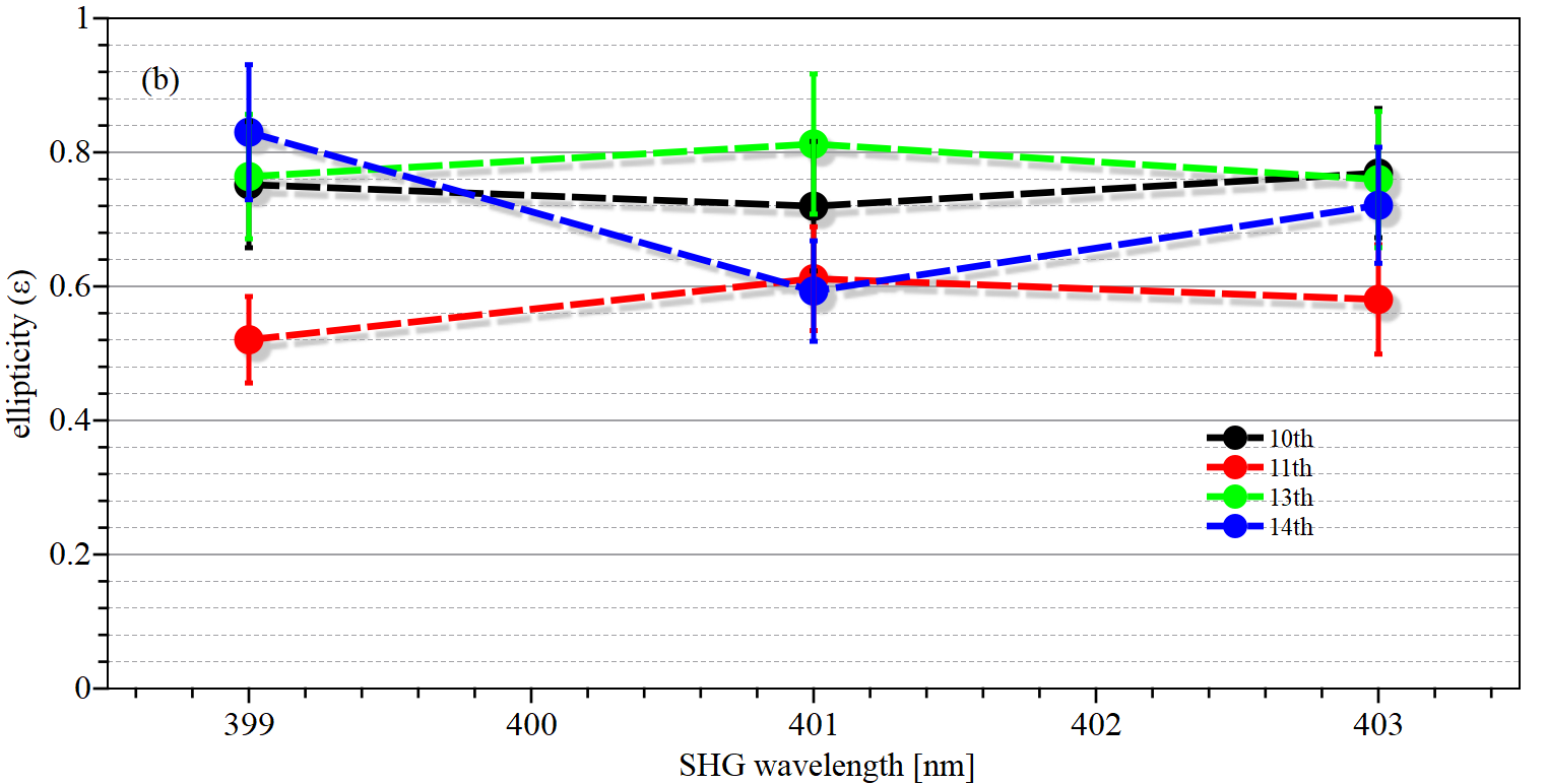
Figure 4: (a)The dependence of ellipticity on the central wavelegth of the SHG of the fundamental frequency at the detection area and (b)the reconsructed ellipticity values at the source .

III.3 Energy Content estimation

The energy content estimation of the XUV radiation was estimated by applying the experimental procedure similar to the one reported in Vassakis et al. (Vassakis et al., 2021) and it was found to be E^XUV$\HF$400 nJ per XUV pulse at the source. Briefly, the energy of the highly elliptical XUV radiation emitted per pulse is estimated at a first step by measuring the linearly polarized XUV pulse energy by means of an XUV photodiode and comparing the HHG spectra depicted in the measured photoelectron spectrum of Ar atoms upon interaction with highly elliptically and linearly polarized XUV light (see Fig. 5) at the same detection conditions. Additionally, the single-photon photoelectron angular distributions were taken into account for each highly elliptical harmonic in the case of Ar(Schönhense, 1980) and in order to check how they affect the detection in the case of our experimental configuration. From all the above, we can deduce the energy per pulse of the highly-elliptical XUV emission. This major improvement with respect to the previous reported value ($\HF$100 $nJ$ at the source)(Vassakis et al., 2021) was due to the improvement of the focusing conditions and the increased input laser energy (32 mJ) of the TW 10 Hz laser system. It should be stressed that no depletion of the atomic target (Ar) was observed during these experimental investigations and therefore higher energy content of highly elliptical XUV radiation is expected by increasing the input energy, therefore the limit for the driving laser energy was set by the possible damage threshold of the optical components. The estimated number of photons per harmonic per pulse at the source is shown in Table 2

Harmonic order	Number of photons per pulse
11th	$\sim$1.4x1010
13th	$\sim$8.4x1010
14th	$\sim$8x109
16th	$\sim$2.3x109
17th	$\sim$3.2x108

Table 2: Number of photons per harmonic order per pulse at the source when Ar is used as generating medium.

III.4 The Semiclassical analysis of HHG spectra and phases

According to the semi-classical approach, the HHG from bi-circular harmonic fields has different characteristics compared to the case of linear monochromatic polarized driver fields. It was shown in (Milosevic et al., 2000) that the main contribution to the harmonic emission comes from electrons with Re(t)<$\nicefrac{{T_{L}}}{{3}}$ (where$T_{L}$is the fundamental laser period). Here it should be stressed that because of the threefold electric field which is raised by the superposition of the bi-circular electric fields, only one trajectory mostly contribute during the process of HHG, in contrast to the case of linear monochromatic drivers where two trajectories contribute to harmonic emission, namely short and long (Kruse et al., 2010; Balcou et al., 1997; Bellini et al., 1998; Peatross and Meyerhofer, 1995).

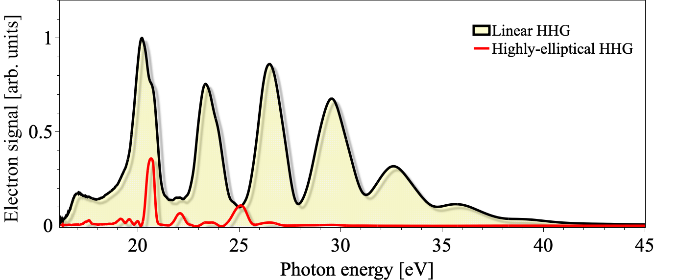
Figure 5: Typical PE spectra of Ar induced by the linear p-polarized and highly-elliptical XUV radiation generated by Ar at the same detection conditions, after the optimization of harmonic emission is realized in both cases.

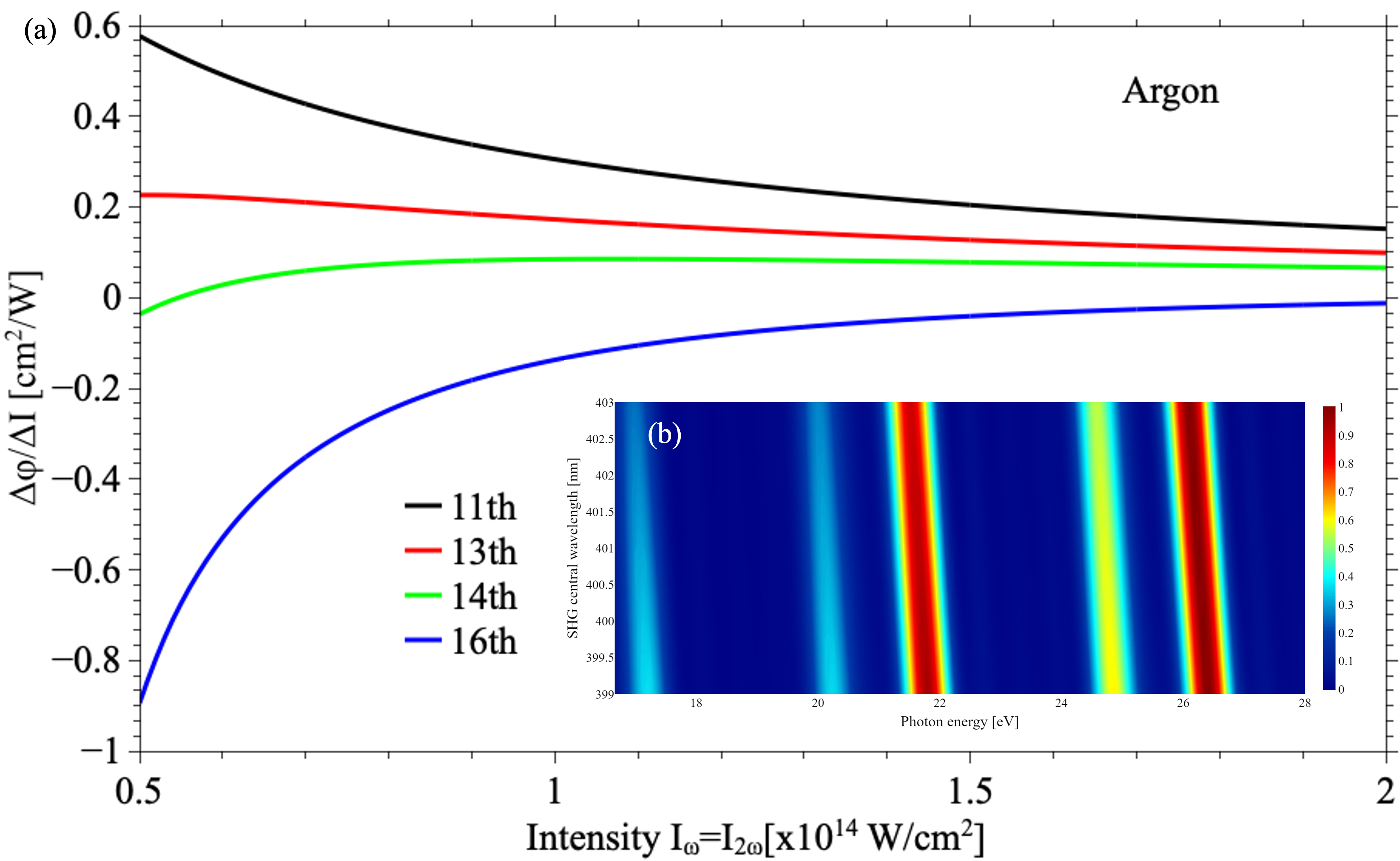
Figure 6: (a) Harmonic phase of the 3n$\pm$1 harmonics (n=4,5) as a function of the intensity of the two components of the bi-circular counter rotating fields. Parameters used in the calculations: laser central wavelength 800 nm, 400nm second harmonic, pulse peak intensity $I_{\omega}=I_{2\omega}$, Argon. (b) Harmonic spectra as as a function of the SHG central wavalength. Parameters used in the calculations: fundamental central wavelength $\lambda_{1}$ = 800 nm and tuning the second harmonic central wavelength between 399 nm$\leq\lambda_{2}\leq$403 nm , pulse peak intensity $I_{\omega}=I_{2\omega}$=1×10¹⁴ W/cm², Argon.

Fig. 6 (a)represents the harmonic phase of the 3n$\pm$1 harmonics (n = 4,5,6) as a function of the intensity in the case where $\text{I}_{\omega}$=$\text{I}_{2\omega}$ of the two components of the bi-circular counter rotating fields. Ar atomic target is used as the generation medium. The result is that the slope of the phase as a function of the intensity for each harmonic is small. This is indicative of a strong collective response when loose focusing geometry is applied(Fleischer et al., 2014; Kfir et al., 2015; Orfanos et al., 2019, 2020; Tzallas et al., 2005). For equal intensities of the laser field components $I_{\omega}=I_{2\omega}$ the cutoff law is $E_{max}$=1.2$I_{p}$+3.17$U_{p}$, where $U_{p}$=$U_{p\omega}$+$U_{p2\omega}$ (Milosevic et al., 2000; Hasović et al., 2016).

Using this semi-classical three step model (Milosevic et al., 2000; Lewenstein et al., 1994) the HHG spectrum was also calculated for different SHG central wavelengths (399 nm $\leq\lambda_{2}\leq$403 nm). It is shown here theoretically (Fig. 6(b)) and verified experimentally in Sec. III.1 that the harmonic photon energy follows a linear dependence on the SHG central wavelength.

III.5 Probing the dynamical origin of the highly ellipticity harmonics with TDDFT

In this work, the peak intensity of the fundamental and the second harmonic fields are taken as $1\times 10^{14}W/cm^{2}$. As shown in Fig. 1(b) the total electric field has a trefoil pattern. The harmonic generation and tunability of the photon energy of the emitted harmonics in Argon atom is obtained by combining a circular polarized light with a fundamental frequency $\omega_{1}$ ($\lambda_{1}$ = 800 nm) with its counter-rotating second harmonic $\omega_{2}$ ($\lambda_{2}$ = 399 nm or 400 nm or 401 nm or 403 nm). The harmonic radiation is plotted as the sum of absolute square of the two polarization components (x and y), as shown in linear and logarithmic-scale in Fig. 7(a) and Fig. 7(b), respectively. The HHG spectrum in Fig. 7(b) displays a distinct structural peak in the lower frequency range of 15-30 eV.

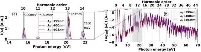
Figure 7: High-order harmonic spectra of an Argon atom in linear scale (a) and logarithmic scale (b) obtained under the influence of BCCR laser field. A wavelength of $\lambda_{1}$ = 800 nm for the fundamental laser field is fixed and the wavelengths of the second harmonic field is varied, i.e. $\lambda_{2}$ = 399, 400, and 403 nm. Energy shift in the high harmonic spectra as a function of second harmonic laser field’s wavelength is shown in panel ’a’.

We find that the emitted harmonic spectral features such as the HHG intensity, polarization states of the harmonics, show strong dependence on the wavelength and intensity ratio of the two driving field components in the BCCR field. The dependence of the generated harmonic spectrum on the SHG central wavelength, as obtained from our TDDFT analysis show very good agreement with the theoretical calculations presented in III.4. A maximum HHG central energy shift of $\sim$150 meV is also observed by tuning the second harmonic wavelength, as shown in Fig. 7a supporting the experimental results of III.1.

We investigate how the ellipticity of the emitted harmonics varies as a function of second harmonic wavelength. For illustration purpose we show for $\lambda_{2}\leavevmode\nobreak\ =\leavevmode\nobreak\ 401$ nm the ellipticity of the 14th emitted harmonics in Fig. 8(a). As shown in Fig. 8(b),a super-Gaussian filter is applied around the 14th harmonic field (red curve) of which is shown in Fig. 8(c). A slice at the peak the harmonic field is selected and an ellipse is fitted to it (blue dashed curve). By taking the ratio of semi-minor and semi-major axis, the ellipticity is calculated. The dependence of second harmonic field wavelength on the ellipticity of the emitted harmonics is shown in Fig. 8(d).

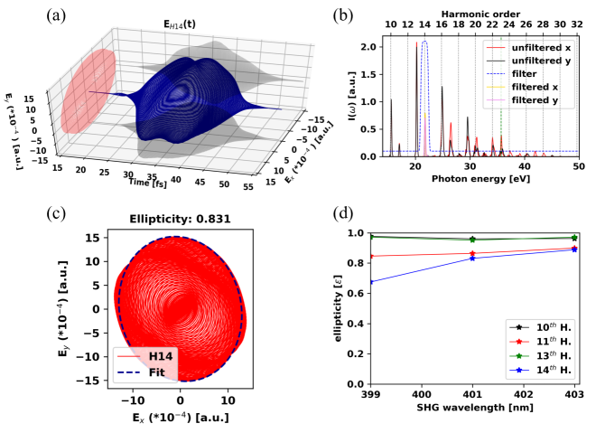
Figure 8: High harmonic generation from Argon using a BCCR laser field with $\lambda_{1}$ = 800 nm and $\lambda_{2}$ = 401 nm. (a) Temporal evolution of the ellipticity of the emitted Harmonics super-Gaussian filtered around 14^th harmonic. (b) Computed HHG spectrum from Argon, Super-Gaussian filtered (blue curve) around 14^th harmonic. The green colored vertical dashed line is the harmonic cutoff. (c) The resulting harmonic field of the filtered harmonics (in red) is sliced at its maximum and fitted to an ellipse (in blue).(d) Effect of second harmonic frequency on the ellipticity of the harmonics

We observe that by using the peak intensities of the fundamental field ($1\times 10^{14}\leavevmode\nobreak\ W/cm^{2}$), the harmonic ellipticity corresponding to the BCCR field induced HHG emission is significantly reduced for all harmonic orders detectable in TOF spectrometer, indicating prominent depolarization effects. In particular, by examining harmonic orders 10^th to 14^th (see Fig. 8d), we find that the calculated ellipticity varies from 0.65–0.98, same as in our experimental results, without showing any predictable particular order, while 10^th and 13^th harmonic show close-to-circularity elliptic nature. Estimated degree of polarization of individual harmonic orders exhibit similar gross features and magnitudes to that obtained from our experimental results.

The difference of the harmonics ellipticity values derived from the experimental data in Fig. 4 and those extracted from the TDDFT calculations in Fig. 8(d) can be attributed to different factors related to the HHG process itself and also in deviations from the optimal experimental conditions. Lou Barreau et al. (Barreau et al., 2018) showed that the breaking of the dynamical symmetry of the three atto-pulses in the $\omega$ cycle (which is the case of when the two color counter-rotating driving fields are applied) would result in a decreased harmonic ellipticity, emission of the 3q harmonic orders and possibly depolarization. This kind of breaking can be induced either by the driving fields imperfect circular polarizations(Milosevic et al., 2000; Fan et al., 2015) , due to imperfect overlap(Álvaro Jiménez-Galán et al., 2017) or by the anisotropic generating medium.(Baykusheva et al., 2016; Yuan and Bandrauk, 2018) Note that macroscopic effects can further affect the polarization of the harmonics (Antoine et al., 1996; Kfir et al., 2015).

IV Conclusions

In conclusion, we report a method to produce tunable energetic highly-elliptical XUV radiation. The approach is based on gas-phase HHG driven by two-color bi-circular polarized fields, produced by a MAZEL–TOV-like device. The approach is applied in the linearly polarized MW XUV beamline at FORTH-IESL, under loose focusing conditions. By properly tuning the central frequency of the second harmonic of the fundamental frequency, the central frequency of the XUV HHG can be continuously tuned. By performing polarimetric measurements ellipticities up to $\sim 85$% at $\sim$22 eV were achieved. No clear dependence on the BBO angle of rotation was observed. The energy per driving laser pulse, in the spectral region $\HF$20 eV, was found to be in the range of E^XUV$\HF$400 nJ per laser pulse at the source. The maximum energy shift observed was $\Delta$E$\HF$150 meV which is in good agreement with the theoretical calculations.

Overall, by combining of state-of-the-art experiments, semi-classical analysis and TDDFT simulations, we demonstrate efficient generation and characterization of highly energetic and elliptic high harmonic spectra from Argon, and also identify the dynamical origin and spectral, temporal nature of the generated elliptic high order harmonics. We find that the proposed technique to generate and tune the BCCR field under suitable focusing conditions can result in highly energetic ( 400 nJ at the source) elliptically polarized harmonic spectra, with a linear dependence of the central HHG energy on the central wavelength of the SHG. While certain harmonics regions demonstrate a high degree of ellipticity (almost tending to circularity, for example, 10^th or 13^th harmonics), other detectable high harmonics demonstrate lower ellipticity. Similar features are also confirmed with our TDDFT simulations. By suitably tuning and improving the focusing conditions, we could achieve a high value of the energy content per pulse of the highly-elliptical XUV emission ( 400 nJ at the source), which is much higher than previously reported results. Hence, employing our approach based on short pulse driving laser, and by varying the SHG central wavelength, it is possible to achieve spatially varying elliptically polarized high harmonics that can be utilized in imaging and spectroscopic applications in the materials Chatziathanasiou et al. (2019), chemical, and nano sciences Kahaly and Waghmare (2008), as well as to probe the chirality sensitive processes.

Supplementary Material

IV.1 BBO Crystal spectral characteristics

The BBO crystal is mounted on a high precision motorized rotational stage and the spectral properties of the SHG can be tuned as a function of the turning angle $\Delta$$\vartheta$ with respect to the propagation axis of the 25-fs IR laser pulse. For a monochromatic fundamental wave, the turning angle corresponds to the phase-mismatching angle at the given fundamental wavelength. For a broadband laser pulse, however, the turning angle means the variation in the phase-matching angle, and the central SHG wavelength is subsequently tuned with respect to the phase-matching angle.

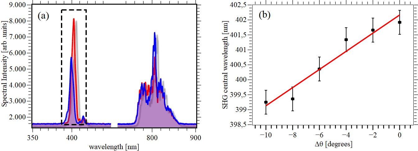
Figure 9: (a)Spectral distributions of the fundamental and SHG pulses for the two extreme positions of the turning angle $\Delta$$\theta$ with the propagation axis of the 25-fs IR laser pulse.(b) SHG central wavelength as a function of angle $\Delta$$\theta$.

It was verified experimentally (Fig. 9(b)) that the central wavelength of the SHG pulse varies linearly with the turning angle $\Delta$$\theta$, and the wavelength variation $\Delta\lambda$₂ of the SHG pulse can be approximately expressed as $\Delta$$\lambda$₂$\HF$0.3 $\Delta$$\theta$ ($-10^{o}\leq\Delta\theta\leq 0^{o}$) for the BBO (0.2 mm, cutting angle 29.20 for type I phase matching) used in the experiment. The corresponding spectral distributions of the fundamental and SHG for two extreme positions of the turning angle $\Delta$$\theta$ are shown in Fig. 9(a).

IV.2 Polarization - Reflective polarizer - Proof of equations used

The ellipticity of the highly elliptical XUV radiation produced through HHG was extractedusing the XUV polarimeter. The analysis of the polarization state of the incident light is achieved via a EUV reflective polarization analyzer, which functions as a non-ideal linear polarizer/analyzer. The polarization of light and its control are often described using Jones vectors and matrices. Jones vectors describe the polarization state of light. Jones matrices describe the effect of different optical devices and processes on the polarization state. They are operators that act on the incoming Jones vector and produce the out-coming Jones vector. The electric field of a monochromatic (of angular frequency $\omega$) plane electromagnetic wave propagating along the z axis can be written as:

$$\left(\begin{array}[]{c}E_{x}(t)\\ E_{y}(t)\\ 0\end{array}\right)=\left(\begin{array}[]{c}E_{0x}(t)e^{i(kz-\omega t+\varphi_{x})}\\ E_{0y}(t)e^{i(kz-\omega t+\varphi_{y})}\\ 0\end{array}\right)=\left(\begin{array}[]{c}E_{0x}(t)e^{i\varphi_{x}}\\ E_{0y}(t)e^{i\varphi_{y}}\\ 0\end{array}\right)e^{i(kz-\omega t)}$$ (4)

where $k=\omega/c$.

The Jones vector is defined as the vector $\left(\begin{array}[]{c}E_{0x}(t)e^{i\varphi_{x}}\\ E_{0y}(t)e^{i\varphi_{y}}\\ 0\end{array}\right)$, or simply

$$\left(\begin{array}[]{c}E_{0x}(t)e^{i\varphi_{x}}\\ E_{0y}(t)e^{i\varphi_{y}}\end{array}\right)$$ (5)

Linearly polarized light occurs when the direction of the electric field remains constant, which means that the plane of polarization (defined by the electric field and the direction of propagation) is constant (or more precisely, parallel to the same plane). Linearly polarized light at an angle $\theta$ with the x axis is described by the Jones vector $\left(\begin{array}[]{c}cos\theta\\ sin\theta\end{array}\right)$ as $\varphi_{x}-\varphi_{y}$ must be zero or an integer multiple of $\pi$.

Elliptically polarized light (with circular polarization being a special case) is generally described by the Jones vector

$$\left(\begin{array}[]{c}E_{0x}(t)\\ E_{0y}(t)e^{i\epsilon}\end{array}\right)$$ (6)

The field vector describes an ellipse on the transverse plane (i.e. the plane perpendicular to the direction of propagation). Special case of elliptically polarized light is circularly polarized (CP) light. Right hand CP light is described by the Jones vector $\frac{1}{\sqrt{2}}\left(\begin{array}[]{c}1\\ -i\end{array}\right)$ and left hand CP light is described by the Jones vector $\frac{1}{\sqrt{2}}\left(\begin{array}[]{c}1\\ i\end{array}\right)$.

Changes in the state of polarization can be achieved via several physical processes, such as reflection, scattering, refraction, and transmission. As previously mentioned, an optical element that transforms the polarization state into another is described by the Jones matrix acting on the incoming Jones vector:

$$\left[\begin{array}[]{c}E_{x}^{{}^{\prime}}\\ E_{y}^{{}^{\prime}}\end{array}\right]=\left[\begin{array}[]{cc}M_{11}&M_{12}\\ M_{21}&M_{22}\end{array}\right]\left[\begin{array}[]{c}E_{x}\\ E_{y}\end{array}\right]$$ (7)

IV.2.1 Jones matrix for a polarizer

A linear polarizer does not affect the vibration direction of either $E_{x}$ or $E_{y}$ . This means that in 7 $M_{12}=M_{21}=$0 and $\begin{array}[]{c}E_{x}^{{}^{\prime}}=p_{x}E_{x}\\ E_{y}^{{}^{\prime}}=p_{y}E_{y}\end{array}$, $0\leq p_{x},p_{y}\leq 1$. Thus, the Jones matrix is written as:

$$J_{p}=\left[\begin{array}[]{cc}p_{x}&0\\ 0&p_{y}\end{array}\right]$$ (8)

where we set$M_{12}=p_{x}$ and $M_{21}=p_{y}$.

For an ideal horizontal polarizer, $J_{p}=\left[\begin{array}[]{cc}1&0\\ 0&0\end{array}\right]$, while for an ideal vertical polarizer $J_{p}=\left[\begin{array}[]{cc}0&0\\ 0&1\end{array}\right]$. For a non-ideal polarizer both $p_{x}$ and $p_{y}$ have non zero values, but one is usually much smaller than the other. When a linear polarizer is rotated by an angle $\frac{\theta}{}$ then the Jones matrix needs to be accordingly rotated, using the rotation matrix. R=$\left[\begin{array}[]{cc}\cos\theta&\sin\theta\\ -\sin\theta&\cos\theta\end{array}\right]$ , i.e.

$$J_{p}(\theta)=R^{-1}J_{p}R=\left[\begin{array}[]{cc}\cos\theta&-\sin\theta\\ \sin\theta&\cos\theta\end{array}\right]\left[\begin{array}[]{cc}p_{x}&0\\ 0&p_{y}\end{array}\right]\left[\begin{array}[]{cc}\cos\theta&\sin\theta\\ -\sin\theta&\cos\theta\end{array}\right]=\left[\begin{array}[]{cc}p_{x}\cos^{2}\theta+p_{y}sin^{2}\theta&(p_{x}-p_{y})\sin\theta\cos\theta\\ -(p_{x}-p_{y})\sin\theta\cos\theta&p_{x}\sin^{2}\theta+p_{y}\cos^{2}\theta\end{array}\right]$$ (9)

For the ideal case, for a horizontal polarizer, $p_{x}=1$ and $p_{y}=0$ and hence the Jones matrix becomes

$$J_{p}(\theta)=\left[\begin{array}[]{cc}\cos^{2}\theta&-\sin\theta\cos\theta\\ -\sin\theta\cos\theta&\sin^{2}\theta\end{array}\right]$$ (10)

Polarization by reflection can be described by the Jones matrix of a non-ideal lineal polarizer.

IV.2.2 Malus’ law for an ideal and a real linear polarizer

Let us assume that the incident electric field is linearly polarized along the x axis, and can be described by the Jones vector $\left(\begin{array}[]{c}1\\ 0\end{array}\right)$. Then, according to 10 the resulting Jones vector will be given by $\left[\begin{array}[]{cc}\cos^{2}\theta&-\sin\theta\cos\theta\\ -\sin\theta\cos\theta&\sin^{2}\theta\end{array}\right]\left(\begin{array}[]{c}1\\ 0\end{array}\right)=\left(\begin{array}[]{c}\cos^{2}\theta\\ -\sin\theta\cos\theta\end{array}\right)$.Where, amplitude of the emerging electric field will be therefore equal to $E_{ox}\cos\theta\sqrt{\cos^{2}\theta+\sin^{2}\theta}$ and hence the intensity of light ($\propto E^{2}$) will be given by

$$I=I_{0}\cos^{2}\theta$$ (11)

which is Malus law for an ideal linear polarizer.

For a non-ideal polarizer, Malus law can be generalized using 9 instead of 10, as follows:

$$\left[\begin{array}[]{c}E_{x}^{{}^{\prime}}\\ E_{y}^{{}^{\prime}}\end{array}\right]=\left[\begin{array}[]{cc}p_{x}\cos^{2}\theta+p_{y}sin^{2}\theta&(p_{x}-p_{y})\sin\theta\cos\theta\\ -(p_{x}-p_{y})\sin\theta\cos\theta&p_{x}\sin^{2}\theta+p_{y}\cos^{2}\theta\end{array}\right]\left(\begin{array}[]{c}1\\ 0\end{array}\right)=E_{0x}\left(\begin{array}[]{c}p_{x}\cos^{2}\theta+p_{y}sin^{2}\theta\\ -(p_{x}-p_{y})\sin\theta\cos\theta\end{array}\right)$$ (12)

and

$$I=I_{0}\left(p_{x}\cos^{2}\theta+p_{y}sin^{2}\theta\right)^{2}+\left((p_{x}-p_{y})\sin\theta\cos\theta\right)^{2}=I_{0}\left[p_{x}\cos^{2}\theta+p_{y}\sin^{2}\theta\right]$$ (13)

This can also be re-written using the extinction ratio

$$R=\frac{p_{x}^{2}}{p_{y}^{2}}$$ (14)

as $I=I_{0}p_{x}\left[\cos^{2}\theta+R\sin^{2}\theta\right]$, which becomes identical to 11 for $p_{x}=1$ and $p_{y}=0$.

IV.2.3 Malus law for a EUV reflective analyzer

13 can be further generalized, if the polarizer (as is the case with the reflective analyzer developed in FO.R.T.H.-I.E.S.L. and utilized for the polarimetric investigation presented in this manuscript) also causes dephasing between the two components of the electric field. In this case the Jones matrix can be written in the more general form

$$J_{p}=\left[\begin{array}[]{cc}p_{x}e^{i\psi_{x}}&0\\ 0&p_{y}e^{i\psi_{y}}\end{array}\right]$$ (15)

We shall assume that the incident light is elliptically polarized as in 6 which can be equivalently written in the form

$$\left(\begin{array}[]{c}E_{0x}(t)e^{i\epsilon/2}\\ E_{0y}(t)e^{-i\epsilon/2}\end{array}\right)$$ (16)

Following the same methodology, we can write for the emerging field:

$$\left[\begin{array}[]{c}E_{x}^{{}^{\prime}}\\ E_{y}^{{}^{\prime}}\end{array}\right]=\left[\begin{array}[]{cc}p_{x}e^{i\psi_{x}}\cos^{2}\theta+p_{y}e^{i\psi_{y}}sin^{2}\theta&(p_{x}e^{i\psi_{x}}-p_{y})\sin\theta\cos\theta\\ -(p_{x}e^{i\psi_{x}}-p_{y}e^{i\psi_{y}})\sin\theta\cos\theta&p_{x}e^{i\psi_{x}}\sin^{2}\theta+p_{y}e^{i\psi_{y}}\cos^{2}\theta\end{array}\right]\left(\begin{array}[]{c}E_{0x}(t)e^{i\epsilon/2}\\ E_{0y}(t)e^{-i\epsilon/2}\end{array}\right)$$ (17)

The intensity is then proportional to

$$I(\theta,\varepsilon)\propto E_{x}^{{}^{\prime}2}+E_{y}^{{}^{\prime}2}=p_{x}^{2}\left[E_{0x}^{2}(\cos^{2}\theta+R\sin^{2}\theta)+E_{0y}^{2}(R\cos^{2}\theta+\sin^{2}\theta)+E_{0x}^{2}E_{0y}^{2}(R-1)\sin 2\theta\cos\varepsilon\right]$$ (18)

where, R is given by 14 .

One can use 18 to derive the ratio $E_{0y}/E_{0x}$ for the incident light, from the measured distribution of intensity as a function of $\theta$, by noting the values of I at $\theta=0(I_{1})$ and $\theta=\pi/2(I_{2})$:

$$I_{1}\propto p_{x}^{2}\left[E_{0x}^{2}+RE_{0y}^{2}\right]$$ (19)

$$I_{2}\propto p_{x}^{2}\left[E_{0x}^{2}R+E_{0y}^{2}\right]$$ (20)

where $\beta=\frac{E_{0x}^{2}}{E_{0y}^{2}}$.

So

$$\frac{E_{0x}}{E_{0y}}=\sqrt{\frac{R-c}{cR-1}}$$ (21)

,with $c\equiv contrast=\frac{I_{1}}{I_{2}}$ .

IV.3 TDDFT setup

The exponential of the Hamiltonian is calculated using LANCZOS method given in Castro et al. (Castro et al., 2004) and the XC potential is represented by the local density approximation (LDA) (Marques et al., 2012; Onida et al., 2002). All the calculations were performed using fully relativistic Hartwigsen, Goedecker, and Hutter (HGH) pseudopotentials (Hartwigsen et al., 1998). To understand the multielectron dynamics of Argon, single Ar atom is placed in a parallelepiped simulation box of size 40 Bohr along each of the three (x,y,z) cartesian directions, which includes 4 Bohr of absorbing regions on either sides of the Argon. The absorbing regions are treated using well-recognized mask function (Koushki et al., 2018; Joachain et al., 2011; Mauger et al., 2019), that ensures prevention of unphysical reflection of field-accelerated electrons at the border of the simulation box. The real-space cell was sampled along all the three directions by a grid spacing of 0.18 Å.

IV.4 The Semiclassical analysis of HHG spectra and phases

In order to have an intuitive picture of the HHG by two color bi-circular polarized fields, we performed calculations based on the semicalssical approach where the theoretical framework and detailed analysis can be found elsewhere (Milosevic et al., 2000). Here we present an abbreviated analysis which is based on Strong Field Approximation (SFA)(Lewenstein et al., 1994) adapted in the case of these electric fields.

Within this model, the radiation at orders 3n$\pm 1$ (with n=1,2,3,…), emitted from a single atom exposed to a intense bi-chromatic driving electric field E(t) with the associated vector potential A(t) $=-\int\mathbf{E}(t)dt$ can be fully characterized by the Fourier transform of the time-dependent dipole moment.

$$\mathbf{x}(\omega)=-i\int_{-\infty}^{\infty}\left\langle\varPsi(t)|\hat{\mathbf{x}}|\varPsi(t)\right\rangle e^{-i\omega t}dt=$$

$$=-i\int_{-\infty}^{\infty}dt{}_{r}\int_{-\infty}^{t_{r}}dt_{i}\int d^{3}\mathbf{p}\times[\mathbf{d}^{\ast}(\mathbf{p}-\mathbf{A}(t_{r}))\cdot\mathbf{E}(t_{i})]$$

$$\mathbf{d}(\mathbf{p}-\mathbf{A}(t_{i}))\times e^{-iS(\mathbf{p},t_{i},t_{r})}+c.c.]$$ (22)

In eq. 22, $\left|\Psi(t)\right\rangle$ denotes the time-dependent wave function of the electron that evolves according to the Schrodinger’s equation, and $\mathbf{\hat{x}=-r}$ is the dipole operator. The temporal integration leads to an integration over the three-dimensional momentum of the active electron $\mathbf{p}$, the ionization time t_i, and recombination time t_r. Moreover, $d(p)=\left\langle p\right|r\left|\psi\right\rangle$ is the dipole matrix element, with the initial bound state $\left|\psi\right\rangle$ and a plane-wave state of momentum p, $\left|\psi\right\rangle=e^{-ipr}$ and for the case of the hydrogen-like atoms can be approximated as(Lewenstein et al., 1994):

$$\mathbf{d}(\mathbf{p})=i(\frac{1}{\pi\alpha})^{\nicefrac{{3}}{{4}}}\frac{\mathbf{p}}{\alpha}e^{-\frac{p^{2}}{2\alpha}}$$ (23)

where $\alpha$ takes the value in the order of $I_{p}$ which is the ionization potential of the atomic target.

In the exponent of eq. 22 the quantity S denotes the quasi-classical action that the active electron experiences during its excursion:

$$S(\mathbf{p},t_{i},t_{r})=\int_{t_{i}}^{t_{r}}dt^{\prime\prime}(\frac{[p-A(t^{\prime\prime})]}{2}+I_{p})$$ (24)

Since the quasi-classical action in eq. 24 varies much faster than the other factors, it is not necessary to solve the five dimensional integral for the dipole moment but we can limit the evaluation of the integral over to the stationary point of the classical action, $\nabla_{p}S(\mathbf{p_{s}},t_{i},t_{r})=0$, where the quantity $\mathbf{p_{s}}$ is the stationary value of the momentum, which can be obtained by equating the derivative of the action in eq. 24with respect to $\mathbf{p}$ to zero. The complex phase is given by the equation:

$$\Theta(\mathbf{p_{s}},t_{i},t_{r})=\omega t_{r}-S(\mathbf{p_{s}},t_{i},t_{r})$$ (25)

Saddle-point approximation (SPA) requires the solution of the saddle-point equations Nayak et al. (2019),obtained by equating the derivatives of eq. 25 with respect to $t_{i}$and $t_{r}$ to zero.

$$\nabla_{p}S(\mathbf{p_{s}},t_{si},t_{sr})=x(t_{sr})-x(t_{si})=0$$ (26)

$$\frac{\partial\Theta(\mathbf{p_{s}},t_{i},t_{r})}{\partial t_{i}}\mid_{t_{si}}=\frac{1}{2}[\mathbf{p_{s}}-\mathbf{A}(t_{si})]^{2}+I_{p}$$ (27)

$$\frac{\partial\Theta(\mathbf{p_{s}},t_{i},t_{r})}{\partial t_{i}}\mid_{t_{sr}}=-\frac{1}{2}[\mathbf{p_{s}}-\mathbf{A}(t_{si})]^{2}-I_{p}+\omega$$ (28)

where all energies are expressed in terms of the photon energy, and the right-hand side of eq. 28 denotes the energy corresponding to photons with frequency $\omega$. Eq. 26 indicates that the only relevant electron trajectories are those where the electron leaves the atom at time t_si and returns at time t_sr. Equation 27 describes energy conservation in the process of tunneling Nayak et al. (2019), where the electron must have a negative kinetic energy at t_si, leading to a complex value of t. Finally, eq. 28 is the energy conservation law at the moment of recombination.

Using the stationary phase approximation Chatziathanasiou et al. (2019), the Fourier transform of the dipole moment, x($\omega$) (eq. 22) can be written as a coherent superposition of the contributions from the complex electron quantum paths corresponding to the complex saddle-point solutions $(\mathbf{p_{s}},t_{si},t_{sr})$. In the spirit of Feynman’s path integrals (Salières et al., 2001) , can be expressed as:

$$\mathbf{x}(\omega)=\underset{s}{\sum}\frac{i2\pi}{\sqrt{det(S^{\prime\prime})}}[\frac{\pi}{\varepsilon-i\frac{(t_{sr}-t_{si})}{2}}]^{\nicefrac{{3}}{{2}}}\mathbf{d^{\ast}}(\mathbf{p}_{s}-\mathbf{A}(t_{sr}))$$

$$\times[\mathbf{\mathbf{E}(t_{si})\cdot d}(\mathbf{p_{s}}-\mathbf{A}(t_{si}))]\times e^{-iS(\mathbf{p},t_{si},t_{sr})+\omega t_{sr}}]$$ (29)

where $det(S^{\prime\prime})$ is the determinant of the 2×2 matrix of the second derivatives of $\Theta(\mathbf{p_{s}},t_{i},t_{r})$ (See eq. 25) with respect to t_i and t_r and the term $[\frac{\pi}{\varepsilon-i\frac{(t_{sr}-t_{si})}{2}}]^{\nicefrac{{3}}{{2}}}$ is related to the wave-packet spreading (Sansone et al., 2004).