Highlighting Object Category Immunity for the Generalization of Human-Object Interaction Detection

Abstract

Human-Object Interaction (HOI) detection plays a core role in activity understanding. As a compositional learning problem (human-verb-object), studying its generalization matters. However, widely-used metric mean average precision (mAP) maybe not enough to model the compositional generalization well. Here, we propose a novel metric, mPD (mean Performance Degradation), as a complementary of mAP to evaluate the performance gap among compositions of different objects and the same verb. Surprisingly, mPD reveals that previous state-of-the-arts usually do not generalize well. With mPD as a cue, we propose Object Category (OC) Immunity to advance HOI generalization. Concretely, our core idea is to prevent model from learning spurious object-verb correlations as a short-cut to over-fit the train set. To achieve OC-immunity, we propose an OC-immune network that decouples the inputs from OC, extracts OC-immune representations and leverages uncertainty quantification to generalize to unseen objects. In both conventional and zero-shot experiments, our method achieves decent improvements. To fully evaluate the generalization, we design a new and more difficult benchmark, on which we present significant advantage. The code is available at https://github.com/Foruck/OC-Immunity.

1 Introduction

Human-Object Interaction (HOI) detection recently attracts enormous attention. It is generally defined as detecting $\langle human,verb,object\rangle$ triplets (Chao et al. 2018) from still images, which is a sub-task of visual relationship detection (Lu et al. 2016, 2018). It plays an important role in robot manipulation (Hayes and Shah 2017), surveillance event detection (Lu, Shi, and Jia 2013; Adam et al. 2008), trajectory prediction (Sun et al. 2021; Sun, Jiang, and Lu 2020), video understanding (Pang et al. 2020, 2021), etc.

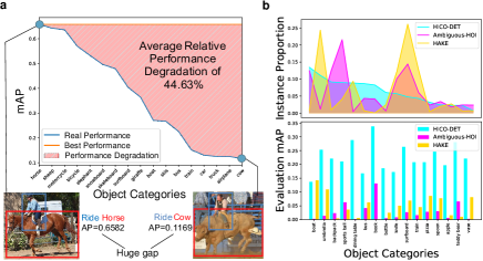
Figure 1: Previous HOI learning methods usually generalize poorly (a) on different object categories; (b) on test set with different object category (OC) distributions. (a). mPD visualization of VCL (Hou et al. 2020) on verb ride. Lower mPD indicates better generalization. (b) Object category distribution and corresponding VCL mAP of different datasets Chao et al. (2018); Li et al. (2020a, 2019b).

Recently, impressive progress has been made in this field (Li et al. 2019c; Hou et al. 2020; Peyre et al. 2019; Li et al. 2020a), and the most widely-used metric mAP (mean Average Precision) has reached an impressive level. However, the compositional generalization problem is still open: they provide limited performance on test samples with the same verbs but rarely seen or unseen object categories. To illustrate this phenomenon more clearly, we propose a novel metric to directly measure generalization in HOI learning, named mPD (mean Performance Degradation). In detail, for a given verb and its available objects, we compute the relative performance gap between the best and the rest verb-object compositions (i.e., the lower, the better). As illustrated in Fig. 1a, previous methods (Hou et al. 2020) usually fail to achieve satisfying mPD, resulting in limited generalization: polarized performances on datasets with diverse object distributions, as shown in Fig. 1b.

Previous methods usually seek HOI generalization from compositional learning (Hou et al. 2020; Bansal et al. 2020). A common way is to import novel objects via language priors (Peyre et al. 2019; Wang et al. 2020; Bansal et al. 2020) and model the similarity between seen and unseen categories, then translate $\langle verb$-$(seen),$ $object$-$(seen)\rangle$ to $\langle verb$-$(seen),$ $object$-$(unseen)\rangle$. This is intuitive but maybe not enough to process the enormous variety: object categories are inexhaustible. Instead, we propose a new perspective: object category (OC) immunity: the performance gap among compositions of different objects for the same verb is a kind of OC-related bias. Due to the imbalanced verb-object distribution, models could learn spurious verb-object correlation as a shortcut to over-fit the training set. To avoid this, we prevent our model from relying too heavily on OC information. This enables it to generalize better to rare/unseen objects. In other words, we adopt OC-immunity to trade-off between fitting and generalization.

In light of this, we propose a new HOI learning paradigm to improve generalization. (1) We introduce OC-immunity, with which the model could rely less on object category and provide better performance for unfamiliar objects. In detail, firstly, we disentangle the inputs of the multi-stream structure (Chao et al. 2018; Li et al. 2019c) from object category. Then, each stream would perform verb classification and uncertainty quantification (Kendall and Gal 2017) concurrently, enabling them to avoid overconfidence when they do not know. Thus, they are expected to be less confident about their mistakes, which is meaningful when encountering unseen objects. (2) For object feature inherently holding category information, we design an OC-immune method via synthesizing object features of different categories as one to mix the category information, thus mitigating the spurious verb-object correlations. Meanwhile, given the compositional characteristic of HOI, the prediction combination of multi-stream is crucial. So we propose calibration-aware unified inference to exploit the unique advantages of different streams. That is, first calibrating streams separately by a variant of Platt scaling (Platt et al. 1999) and then combining multi-prediction regarding uncertainty. (3) As an extra benefit, uncertainty quantification provides an option to utilize data without HOI labels, which can reduce bias and advance generalization. For evaluation, we conduct experiments on HICO-DET (Chao et al. 2018) under both conventional (Chao et al. 2018) and zero-shot settings (Shen et al. 2018; Hou et al. 2020), showing considerable improvements. To further demonstrate the efficacy of our method, we design a benchmark for HOI generalization, on which impressive advantage is also achieved.

Our contribution includes: 1) We propose mean performance degradation (mPD) to quantify HOI generalization. 2) Object category immunity is introduced to HOI learning with a novel paradigm. 3) A novel benchmark is devised to facilitate researches on HOI generalization. 4) Our proposed method achieves impressive improvements for both conventional and zero-shot HOI detection.

2 Related Works

HOI Learning: Large datasets (Chao et al. 2018; Gupta and Malik 2015; Kuznetsova et al. 2020) have been released. Meanwhile, many deep learning-based methods (Gkioxari et al. 2018; Li et al. 2020a; Peyre et al. 2019; Hou et al. 2020; Li et al. 2020c; Fang et al. 2021a, b, 2018a) have been proposed. Chao et al. (2018) proposed multi-stream framework followed by subsequent works (Gao, Zou, and Huang 2018; Li et al. 2019c; Gao et al. 2020; Hou et al. 2020). Qi et al. (2018) and Wang, Zheng, and Yingbiao (2020) used graphical model to address HOI detection. Gkioxari et al. (2018) estimated the interacted object locations. Gao, Zou, and Huang (2018) and Wan et al. (2019) adopted self-attention to correlate the human, object, and context. Li et al. (2019c) modeled interactiveness to suppress non-interactive pairs given human pose (Fang et al. 2017; Li et al. 2019a). Li et al. (2020a) used 3D human information (You et al. 2021) to enhance HOI learning, while Hou et al. (2020) exploited the compositional characteristic of HOI. Also, some works (Peyre et al. 2019; Kim et al. 2020; Zhong et al. 2020) utilized the relationship between HOIs. Liao et al. (2020) and Fang et al. (2018b) directly detected HOI pairs.

Zero-shot HOI Detection has become a new focus recently (Shen et al. 2018; Bansal et al. 2020; Peyre et al. 2019; Hou et al. 2020; Wang et al. 2020). Shen (Shen et al. 2018) first proposed to factorize HOI into verb classification and object classification. Some works (Bansal et al. 2020; Peyre et al. 2019; Wang et al. 2020) utilized language prior to reason about the relationship between objects for zero-shot generalization. Hou et al. (2020) made use of the compositional characteristic of HOI to generate novel HOI types. As described, most of them adopt object knowledge to reason about objects, suffering from inexhaustibility.

Uncertainty Quantification models what a model does not know. There has been increasing literature in uncertainty estimation of deep learning models (Bishop et al. 1995; Kendall and Gal 2017; Gal and Ghahramani 2016; Lee and AlRegib 2020; Blundell et al. 2015; Lee et al. 2015). Some methods (Bishop et al. 1995; Blundell et al. 2015) are based on Bayesian Neural Network, estimating the distribution of network parameters and producing Bayesian approximation of epistemic uncertainty. MC-Dropout (Gal and Ghahramani 2016) sampled a discrete model from Bayesian parameter distribution. Moreover, Kendall and Gal (2017) used direct estimation for aleatoric uncertainty and MC-Dropout for epistemic uncertainty. There has also been ensemble-based methods (Lee et al. 2015) and gradient-based methods (Lee and AlRegib 2020). In this paper, we adopt the aleatoric uncertainty estimation in (Kendall and Gal 2017).

Calibration aims to improve the quality of the output confidence of a model. Platt scaling (Platt et al. 1999) has been shown effective while simple. In this work, we adopt Platt scaling to calibrate the output probability of our model.

3 Method

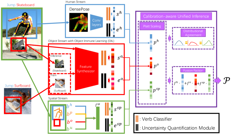
Figure 2: Overview of our pipeline. We design a multi-stream structure facilitated with uncertainty quantification, then calibration-aware unified inference unifies multi-stream into the final prediction $\mathcal{P}$. $s^{h},s^{o},s^{sp}$ are the verb classification logits, and $e^{h},e^{o},e^{sp}$ are the predicted log variances.

In this section, we first formulate the proposed HOI generalization metric. With the metric, our goal is improving generalization by introducing OC-immunity to HOI learning. To this end, we modify the multi-stream structure (Li et al. 2019c; Chao et al. 2018) to realize OC-immunity by disentangling the inputs and devising a new OC-immune learning method. Furthermore, we utilize uncertainty quantification to unify multi-stream concerning calibration.

3.1 Generalization Quantification in HOI

Generalization has been a central obstacle to HOI understanding. Though previous methods (Li et al. 2020a; Hou et al. 2020) provide impressive results of mAP, the generalization performance is still limited in transfer experiments and zero-shot settings (Hou et al. 2020; Bansal et al. 2020; Peyre et al. 2019; Shen et al. 2018). In other words, the relation between mAP and the generalization ability is not as explicit as we expect. This reminds us that widely-used mAP might not be sufficient to evaluate the performance of HOI detection, especially for generalization. To quantify the generalization ability of an HOI learning model, we propose a novel metric, mPD (mean Precision Degradation). For verb $v\in V$, we denote the object categories available for $v$ as $O_{v}$, $AP_{\langle v,o\rangle}$ as the average precision for HOI composition $\langle v,o\rangle$. Then mPD is formulated as:

$$mPD = \frac{1}{|V|}\mathop{\sum}_{v\in V}\frac{AP_{\langle v,o_{max}\rangle}-\bar{AP_{v}}}{AP_{\langle v,o_{max}\rangle}},$$ (1)

where $o_{max}$=$\mathop{\textrm{argmax}}_{o}AP_{\langle v,o\rangle}$, $\bar{AP_{v}}$=$\frac{1}{|O_{v}|}\mathop{\sum}_{o\in O_{v}}AP_{\langle v,o\rangle}$ is the mean AP for compositions $\langle v,o\rangle$ with $o\in O_{v}$. mPD measures performance gap between the best-detected composition and the rest. The higher the mPD is, the larger performance gap a model might present on different objects, in other words, worse generalization. As shown in Fig. 1a and Fig. 6, mPD reveals previous method (Hou et al. 2020) has huge performance gap among different objects with the same verb, which limits generalization. To address this, we utilize OC-immunity as a proxy to narrow the generalization gap.

3.2 OC-Immune Network

The performance gap could result from spurious object-verb correlations learned by model as a short-cut to over-fit the training set. Previous methods intend to achieve generalization by taking more object categories (OC) into consideration with the help of language priors (Hou et al. 2020; Peyre et al. 2019; Bansal et al. 2020), learn the unseen objects via their similarity with the seen objects. However, there exists an inherent limitation: We can not exhaust all the objects due to their variety and visual diversity. While we take this from another view: an inherently OC-immune representation of HOI. The idea is to encourage the model to focus more on interaction-related information instead of OC-related information, thus weakening the influence of object categories. To achieve this, we resort to the multi-stream structure in HOI learning (Chao et al. 2018; Li et al. 2019c). Despite the relatively poor generalization of previous methods, we find this structure has an inherent relation to OC-immunity.

In the multi-stream structure, each stream is designed to perform inference based on one specific element: human, object, or spatial configuration, while the human stream and spatial stream are inherently object-immune by ideal design. However, in previous works, this structure performs poorly as an OC-immune model (Fig. 1a). This is because though the separated streams seem to ignore the object category information, the features used are still entangled with object. Previous works (Chao et al. 2018; Gao, Zou, and Huang 2018; Li et al. 2019c) usually adopt pre-trained object detectors (Ren et al. 2015) as feature extractor, and utilize ROI pooling to get features for different elements. Some of them (Gao, Zou, and Huang 2018; Li et al. 2019c) also enhance spatial stream with human ROI feature. These violate the object-immune principle in two aspects. First, the object detector extracted features are trained to classify object categories, e.g., COCO (Lin et al. 2014) 80 objects, thus inevitably strongly correlated to OC. Second, human and object boxes in HOI pairs usually overlap, therefore, ROI pooling may introduce OC information to human features. To address these violations, we disentangle the feature used by each stream and design different structures for each stream correspondingly, as shown in Fig. 2. Especially, since the object feature inherently holds category information, a new OC-immune learning method is designed for object stream.

Human Stream For human stream, we use COCO (Lin et al. 2014) pre-trained DensePose (Alp Güler, Neverova, and Kokkinos 2018) to extract human feature. It provides a pure geometric encoding of human information, which is totally object-immune. As shown in Fig. 3(a), the conventional ROI pooling feature and DensePose feature distribute diversely, while DensePose feature is more robust to the overlap with objects. We use multiple convolution layers with batch normalization and ReLU activation, followed by global average pooling to encode the input into features, then employ an MLP to perform verb classification.

Object Stream To obtain OC-immune representations, we design a new OC-immune learning method including an object feature synthesizer, an object classifier, and a verb classifier, which are all MLP-based. With two object ROI features as input, the synthesizer outputs a synthesized feature, which is expected to be the intermediate of the two inputs. That is, for example, if we employ the synthesizer to synthesize an object feature with object category labels of “apple” and another with “pear”, the expected result that object classifiers provide for this synthesized vector should be 0.5 for “apple” and “pear”. To achieve this, we first train an object classifier with original data. Then, we freeze the object classifier and train the synthesizer to follow the above rules. Finally, we train our verb classifier with the synthesizer. In detail, for a training object feature, we would randomly duplicate it or sample another object feature of similar object categories (those could be imposed similar verbs, e.g., eating apple and banana), then feed them to the synthesizer and verb classifier, use their intermediate verb label as supervision. In inference, the object feature would be duplicated and fed into the synthesizer and the verb classifier. The idea is to expose the verb classifier to feature with ambiguous or corrupted object category information, while still keeping the verb semantics within the feature. This weakens the correlation between verb and OC that could be perceived by the verb classifier, encouraging the classifier to resort to other clues. Thus, the influence imposed by OC on the verb classifier would be weakened. To show the immunity of our verb classifier, we visualize features extracted by COCO (Lin et al. 2014) pre-trained Faster-RCNN (Ren et al. 2015) and the last FC of our verb classifier in Fig. 3(b). As illustrated, the latter is less correlated with OC than the former.

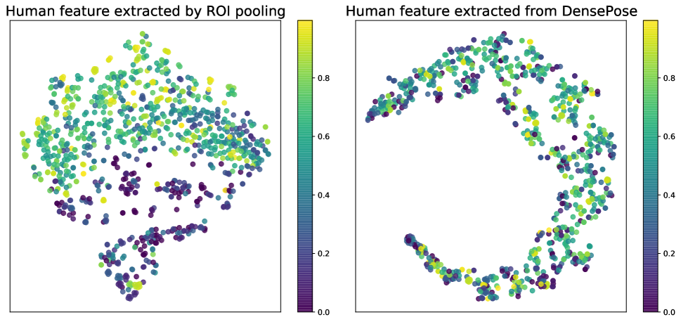
(a) Human feature involving HOI $\it{ride\ bicycle}$, extracted by ROI Pooling and DensePose. The more a human instance overlaps with an object, the brighter it is painted.

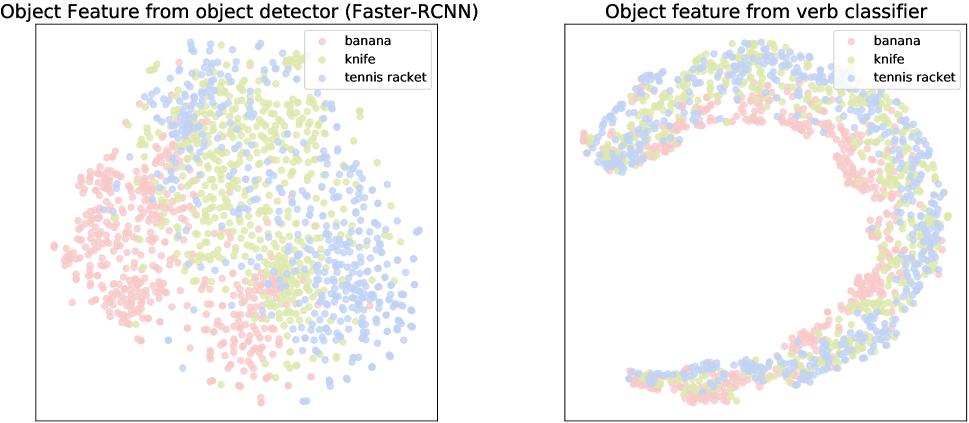
(b) Object feature of $\it{banana},\ \it{knife},\ \it{tennis\ racket}$, from COCO pre-trained Faster-RCNN and the last FC of our verb classifier. Different colors indicate different object categories.

Figure 3: t-SNE (Maaten and Hinton 2008) visualization of differently extracted features.

Spatial Stream Previously, some works (Chao et al. 2018; Li et al. 2019c) directly concatenate human features with spatial configuration features for spatial stream, which violates the object-immune principle as stated before. Therefore, we employ only human and object bounding boxes $b^{h},b^{o}\in\mathbb{R}^{2\times 2}$ and 2D human pose $b^{p}\in\mathbb{R}^{k\times 2}$ to encode the HOI spatial information, where $k$ is the number of human keypoints. We normalize the coordinates of bounding boxes and pose into feature vector $f^{sp}$. In detail, denote the tight union bounding box of $b^{h},b^{o}$ as $b^{u}\in\mathbb{R}^{2\times 2}$ (represented by the upper-left and bottom-right points), we get $f^{sp}$=$\rm{Flatten}(\frac{\rm{concat}(b^{h},b^{o},b^{p})-b^{u}[0,:]}{b^{u}[1,:]-b^{u}[0,:]})$, where $\rm{Flatten}(\cdot)$ indicates the transformation to a vector. Finally, $f^{sp}$ is fed into an MLP to classify the verbs.

Uncertainty Quantification Module Moreover, we corporate an additional MLP as uncertainty quantification module in each stream, following the aleatoric uncertainty estimation in (Kendall and Gal 2017). Each data point is assumed to possess a fixed uncertainty. Then, each stream not only outputs a logit $s$ for verb $v\in V$, but also estimates the uncertainty by log variance $e$. Thus, loss for a sample of verb $v$ is $L^{s}$=$||\frac{\sigma(s)-y}{\exp(e)}||^{2}+\frac{1}{2}e$ following the logistic regression setting in (Kendall and Gal 2017), where $y$ indicates whether sample has verb $v$. Concurrent with the correct prediction, the loss encourages the model to have higher uncertainty on unfamiliar samples while avoiding being uncertain to all the samples. Overall, the model would output higher uncertainty for samples of unfamiliar object categories, thus reduce the overconfident mistakes and advance generalization.

Calibration-Aware Unified Inference. With separately trained three streams, we need to unify them into one final result without loss of immunity and detection performance. Given the inherent compositional characteristic of HOI, it is crucial to explore how to unify multi-stream knowledge. To this end, instead of simple addition or multiplication (Li et al. 2019c; Gao, Zou, and Huang 2018), we propose calibration-aware unified inference as shown in Fig. 2, which exploits the learned uncertainty quantification, imports more flexibility, and preserves unique advantages of each stream. Denote the output logit vectors of three streams as $s^{*}$ and the log variance vectors as $e^{*}$, where $*$ is $h,o$ or $sp$. First, separate calibration is imposed on three streams. Intuitively, the more uncertain a prediction is, the less it should contribute to the final result. Thus, the calibrated prediction of the streams are formulated as $p^{*}$=$Sigmoid(\frac{w^{*}\cdot s^{*}+c^{*}}{\exp(e^{*})})\cdot det^{h}\cdot det^{o}$, $w^{*}$, $c^{*}$ are learnable scaling parameters following (Platt et al. 1999), and $det^{h}$, $det^{o}$ are the object detection confidences from the object detector. The parameters are trained to minimize the BCE loss as Eq. 6 on the validation set, thus helping each separate stream to achieve well-calibration. The objective is formulated as $L^{*}=L_{ent}(p^{*},y)$, $y\in[0,1]^{|V|}$ is the label vector. Second, we impose a distributional agreement loss among the three streams, which is formulated as $L_{agree}=|\rm{mean}\it{(p^{h}_{j}-p^{o}_{j})}|+|\rm{mean}\it{(p^{o}_{j}-p^{sp}_{j})}|+|\rm{mean}\it{(p^{sp}_{j}-p^{h}_{j})}|$, where $p^{h}_{j}$ denotes all the predictions of $p^{h}$ for verb $v_{j}$, the same is for $p^{o}_{j}$ and $p^{sp}_{j}$. This constraint does not require different streams output same value for the same data point like (Li et al. 2020a). Instead, it expects different streams to have similar average outcomes for a set of data points, which is more flexible. Finally, to achieve better overall performance and calibration, we learn fusion factors $f^{h}$, $f^{o}$ and $f^{sp}$ on the validation set, where $f^{h},f^{o},f^{sp}>0$ and $f^{h}$ $+$ $f^{o}$ $+$ $f^{sp}$ = $1$. The final unified inference score is formulated as $\mathcal{P}$=$f^{h}\cdot p^{h}+f^{o}\cdot p^{o}+f^{sp}\cdot p^{sp}$. We use a BCE loss $L_{uni}$=$-(\log(1-\mathcal{P})(1-y)+\log(\mathcal{P})y)$ as the objective. The total calibration loss is formulated as $L_{cal}$=$\beta(L^{h}$+$L^{o}$+$L^{sp})$+$\gamma L_{agree}$+$L_{uni}$, where $\beta$ and $\gamma$ are both weighting factors. The parameters of each stream are frozen during calibration.

Overall, we introduce OC-immunity to the multi-stream structure, encouraging it to be insensitive to object categories while keeping representative to verbs. Thus, our model is robust against different object distributions. Meanwhile, the uncertainty quantification module provides clues on how much the model output could be trusted. It prevents the model from committing over-confident mistakes, boosting its generalization on unfamiliar objects. Finally, the proposed calibration-aware unified inference helps exploit most of each stream in the result, bringing better generalization.

4 Experiment

In this section, we first introduce our uncertainty-guided training strategy. Then, we introduce the adopted datasets, metrics and implementation details. Next, we compare our method with previous state-of-the-arts on multiple HOI datasets (Chao et al. 2018; Li et al. 2020a, 2019b). At last, ablation studies are conducted.

4.1 Uncertainty-Guided Training

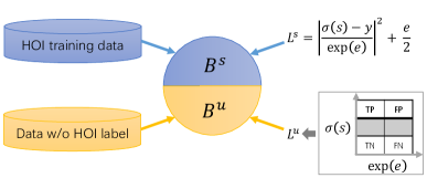
Figure 4: With uncertainty estimation, we are enabled to utilize data without HOI label as an extra benefit.

Besides conventional fully-supervised training, we could enhance our model with data without HOI labels as an extra benefit. Previous methods fail to exploit unlabeled data since only verb predictions are provided, but no clue is there for correctness. While our uncertainty quantification could additionally provide ambiguous but trustworthy pseudo label of correctness, enabling the model to generate pseudo labels for the unlabeled data and further boost both verb classification and uncertainty quantification in a self-training manner. We collect data from validation set of OpenImage (Kuznetsova et al. 2020) as extra unlabeled data and extract the required features for different streams as in Sec. 3. With these, we can operate uncertainty-guided training using unlabeled data as shown in Fig. 4.

A mini-batch $B$ is mixed of labeled data $B^{s}$=$\{b^{s}\}$ and unlabeled data $B^{u}$=$\{b^{u}\}$. For labeled sample $b^{s}\in B^{s}$ and verb $v$, the model outputs logit $s^{s}$ and log variance $e^{s}$. Thus, the loss for $b^{s}$ is calculated following $L^{s}$ as stated before. For unlabeled sample $b^{u}\in B^{u}$ and verb $v$, we define the result evaluation (true positive, false positive, true negative and false negative) with respect to $B^{s}$, then calculate loss $L^{u}$ for them as shown in Fig. 5. First, we compute thresholds $p^{p}$, $p^{n}$, $p^{m}$, $\epsilon$ as Eq. 2-5, where $\sigma(x)=\frac{1}{1+\exp(-x)}$:

$$p^{p} = \max(\mathop{\rm{mean}}_{b^{s},y^{s}=1}(\sigma(s^{s})),\mathop{\max}_{b^{s},y^{s}=0}(\sigma(s^{s}))),$$ (2)

$$p^{n} = \min(\mathop{\rm{mean}}_{b^{s},y^{s}=0}(\sigma(s^{s})),\mathop{\min}_{b^{s},y^{s}=1}(\sigma(s^{s}))),$$ (3)

$$p^{m} = \frac{1}{2}(p^{p}+p^{n}),$$ (4)

$$\epsilon = \mathop{\rm{mean}}_{b^{s}}(\exp(e^{s})).$$ (5)

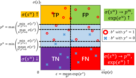
Figure 5: We divide unlabeled samples into TP, TN, FP, and FN according to the output confidence and uncertainty. Based on this, loss is designed to tune the model.

Then, for unlabeled instance $b^{u}$, if $\sigma(s^{u})$ is higher than $\sigma(s^{s})$ of all labeled negative samples ($b^{s}\in B^{s},y^{s}$=$0$) and the mean $\sigma(s^{s})$ of all labeled positive samples ($b^{s}\in B^{s},y^{s}$ = $1$), formulated as $\sigma(s^{u})>p^{p}$, we define it as a positive sample. Similarly, if $\sigma(s^{u})$ is lower than $\sigma(s^{s})$ of all labeled positive samples and the mean $\sigma(s^{s})$ of all labeled negative samples, we define it as a negative sample. Next, if the variance $\exp(e^{u})$ is lower than the mean variance of all labeled samples $b^{s}\in B^{s}$, we define it as a true sample, otherwise a false sample. With these definitions, we construct loss based on BCE loss (Eq. 6) for the unlabeled samples as Eq. 7:

$$L_{e}(p,y)=-(\log(1-p)(1-y)+\log(p)y),$$ (6)

$$L^{u}=\left\{\begin{array}[]{rcl}L_{e}(\sigma(s^{u}),p^{m})-e^{u},&\sigma(s^{u})>p^{p},\sigma(e^{u})>\epsilon,\\ L_{e}(\sigma(s^{u}),1),&\sigma(s^{u})>p^{p},\sigma(e^{u})<\epsilon,\\ L_{e}(\sigma(s^{u}),p^{m})-e^{u},&\sigma(s^{u})<p^{n},\sigma(e^{u})>\epsilon,\\ L_{e}(\sigma(s^{u}),0),&\sigma(s^{u})<p^{n},\sigma(e^{u})<\epsilon,\\ 0,&otherwise\end{array}\right.$$ (7)

The loss is straightforward: For TP/TN samples, we suppose these samples are labeled with corresponding $y^{u}$, and impose BCE loss on them, while we neither punish nor encourage the uncertainty estimation to avoid bias. For FP/FN samples, we expect the model to be uncertain and the prediction to be mediocre. For the samples defined neither positive nor negative, we identify them as unfamiliar samples and impose no loss on them, since they receive expected mediocre prediction. The overall loss of mini-batch $B$ for each stream is represented as $L_{ugt}=\frac{1}{|V|}(\mathop{\sum}\limits_{b^{s}\in B^{s}}\mathop{\sum}\limits_{v\in V}\frac{L^{s}}{|B^{s}|}+\mathop{\sum}\limits_{b^{u}\in B^{u}}\mathop{\sum}\limits_{v\in V}\frac{\alpha L^{u}}{|B^{u}|})$, where $\alpha$ is a weighting factor. With the designed loss, our model could generate trustworthy pseudo-label, regularize the verb classification and uncertainty estimation, and further boost generalization. The corresponding analysis is detailed in Sec. 4.4-4.8.

4.2 Dataset and Metric

We adopt three large-scale HOI detection benchmarks: HICO-DET (Chao et al. 2018), Ambiguous-HOI (Li et al. 2020a), and self-compiled HAKE (Li et al. 2019b) test set. The detailed statistics of the datasets are illustrated in the supplementary material. For all three datasets, we evaluate our HICO-DET trained model using mAP following Chao et al. (2018): true positive should accurately locate human/object and classify the verb. The proposed mPD is evaluated under Default mode on verbs available for multiple object categories.

4.3 Implementation Details

We re-split HICO-DET training set into train set and validation set, roughly a 6:4 split. And we collect 10,434 images from OpenImage validation set (Kuznetsova et al. 2020) as extra unlabeled data, containing 43,553 human instances, 77,485 object instances and 636,649 pairs. In the following, ‘train‘ refers to training on the train set and unlabeled data, while ‘calibrate‘ refers to calibrating on the validation set. All three streams are separately trained by SGD optimizer with learning rate of 7e-3. We train human stream for 50 epochs, the other two for 40 epochs. The unified calibration takes 2 epochs with SGD optimizer, learning rate of 1e-3, $\beta$ = $1$, and $\gamma$ = $0.1$. All experiments are conducted on a single NVIDIA Titan Xp GPU. Please refer to the supplementary material for more details.

4.4 Results on Conventional HOI Detection

	mPD $\downarrow$	mAP Default $\uparrow$			mAP Known Object $\uparrow$
Method		Full	Rare	Non-Rare	Full	Rare	Non-Rare
Shen et al. (2018)	-	6.46	4.24	7.12	-	-	-
HO-RCNN (Chao et al. 2018)	-	7.81	5.37	8.54	10.41	8.94	10.85
Gkioxari et al. (2018)	-	9.94	7.16	10.77	-	-	-
GPNN (Qi et al. 2018)	-	13.11	9.34	14.23	-	-	-
Xu et al. (2019)	-	14.70	13.26	15.13	-	-	-
iCAN (Gao, Zou, and Huang 2018)	0.4699	14.84	10.45	16.15	16.26	11.33	17.73
Wang et al. (2019)	-	16.24	11.16	17.75	17.73	12.78	19.21
TIN (Li et al. 2019c)	0.4313	17.03	13.42	18.11	19.17	15.51	20.26
No-Frills (Gupta, Schwing, and Hoiem 2019)	-	17.18	12.17	18.68	-	-	-
Zhou and Chi (2019)	-	17.35	12.78	18.71	-	-	-
PMFNet (Wan et al. 2019)	-	17.46	15.65	18.00	20.34	17.47	21.20
Peyre et al. (2019)	0.4314	19.40	14.60	20.90	-	-	-
Ulutan, Iftekhar, and Manjunath (2020)	-	19.80	16.05	20.91	-	-	-
DJ-RN (Li et al. 2020a)	0.4121	21.34	18.53	22.18	23.69	20.64	24.60
Ours	0.3836	21.95	20.89	22.27	24.79	23.82	25.08
PPDM (Liao et al. 2020)	0.3930	21.73	13.78	24.10	24.58	16.65	26.84
Bansal et al. (2020)	-	21.96	16.43	23.62	-	-	-
VCL (Hou et al. 2020)	0.4106	23.63	17.21	25.55	25.98	19.12	28.03
IDN (Li et al. 2020b)	0.3876	26.29	22.61	27.39	28.24	24.47	29.37
Ours	0.3905	25.44	23.03	26.16	27.24	24.32	28.11
iCAN (Gao, Zou, and Huang 2018)	0.3441	33.38	21.43	36.95	-	-	-
TIN (Li et al. 2019c)	0.3421	34.26	22.90	37.65	-	-	-
Peyre et al. (2019)	0.3203	34.35	27.57	36.38	-	-	-
VCL (Hou et al. 2020)	0.3097	38.97	29.99	41.65	-	-	-
IDN (Li et al. 2020b)	-	43.98	40.27	45.09	-	-	-
Ours	0.2971	41.32	35.57	43.03	-	-	-

Table 1: Results on HICO-DET (Chao et al. 2018). The first part adopted COCO pre-trained detector. HICO-DET fine-tuned detector is used in the second part. GT human-object pair boxes are used in the last part.

HICO-DET: Quantitative results are demonstrated in Tab. 1, compared with previous state-of-the-art methods using different object detectors. The results are evaluated following Chao et al. (2018): Full (600 HOIs), Rare (138 HOIs), and Non-Rare (462 HOIs) in Default and Known Object mode. Also, we compare mPD with some open-sourced algorithms in Tab. 1. As shown, our method provides an impressive mAP of 21.95 (Default Full) and outperforms all previous algorithms on mPD (0.3836) with COCO (Lin et al. 2014) pre-trained object detector. And it achieves similar performance with IDN (Li et al. 2020b) using HICO-DET fine-tuned object detector and GT human-object pairs. It is even comparable with very recent transformer-based methods (e.g., Kim et al. (2021): mAP 25.73, mPD 0.3978) with much larger capacity.

Ambiguous-HOI (Li et al. 2020a) is adopted to further evaluate our model on unfamiliar data. As shown in Tab. 2, our model provides competitive mAP and considerable improvement on mPD over previous state-of-the-arts, proving its robustness against object category distribution.

HAKE test set: Results are illustrated in Tab. 2. Some previous open-sourced SOTA are compared. We could observe the superior performance of our method even with domain shift, demonstrating the generalization ability of our model.

	Ambiguous-HOI		HAKE test set
Method	mPD $\downarrow$	mAP $\uparrow$	mPD $\downarrow$	mAP $\uparrow$
iCAN (Gao, Zou, and Huang 2018)	0.5060	8.14	0.5324	9.66
TIN (Li et al. 2019c)	0.4890	8.22	0.4792	10.45
Peyre et al. (2019)	0.4935	9.72	0.5132	12.03
DJ-RN (Li et al. 2020a)	0.4800	10.37	-	-
Ours	0.4715	10.45	0.4736	14.26

Table 2: Results comparison on Ambiguous-HOI (Li et al. 2020a) and newly designed test set from HAKE.

4.5 Results on Zero-shot HOI Detection

To demonstrate the generalization ability of our method, we evaluate the performance of our method under zero-shot settings. 120 of the 600 HOI categories in HICO-DET (Chao et al. 2015) are selected as unseen categories (Shen et al. 2018; Hou et al. 2020). We adopt the non-rare first selection (Hou et al. 2020), which is more difficult. Instances of the unseen categories are removed during training, while the test set is unchanged. mAP is reported under three settings (Full, Seen, Unseen) with Default mode. mPD is evaluated for open-sourced methods (Hou et al. 2020) and our method. Comparison is conducted among several previous methods under the same setting. As shown in Tab. 3, our method considerably outperforms previous methods. More experiments are in the supplementary material.

	mPD $\downarrow$	mAP $\uparrow$
Method		Full	Seen	Unseen
Shen et al. (2018)	-	6.26	-	5.62
VCL (Hou et al. 2020)	0.4877	12.76	13.67	9.13
Ours	0.4415	14.80	15.70	11.21
Bansal et al. (2020)	-	12.26	12.60	10.93
VCL (Hou et al. 2020)	0.4531	18.06	18.52	16.22
Ours	0.4194	19.85	20.23	18.34

Table 3: Results of zero-shot HOI detection. The first part adopted COCO pre-trained detector. HICO-DET fine-tuned detector is used for the second part.

4.6 Visualization

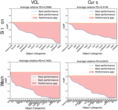
Figure 6: mPD comparison of VCL and ours.

We visualize mPD comparison of VCL (Hou et al. 2020) and ours in Fig. 6. As shown, our method shows similar or even lower best AP while still outperforming VCL (Hou et al. 2020) by providing less performance degradation, implying that we manage to achieve a better trade-off. More visualizations are included in the supplementary material.

4.7 Ablation Study

We conduct ablation studies on HICO-DET (Chao et al. 2018) with COCO (Lin et al. 2014) pre-trained Faster-RCNN (Ren et al. 2015). For more ablation studies please refer to the supplementary material.

OC-immune learning (OIL):. We remove the synthesizer and train the verb classifier directly with raw data. As shown, the performance for Non-rare set barely hurts, while both mPD and Rare mAP decrease substantially. This sustains the effectiveness of OIL in mitigating the performance gap between different objects with same verb.

Uncertainty quantification module (UQM): Its removal results in a 0.52 mAP drop and marginal mPD increase. The performance on Rare hurts more than that on Non-Rare, indicating the importance of UQM for unfamiliar samples.

Calibration-aware unified inference (CUI): If we jump the calibration stage, and directly fuse the three streams, mAP suffers by 0.79, proving the crucial role of CUI.

Extra data: Without the extra data, we get mAP of 20.05 and mPD of 0.3987, which is still competitive. In additional, we achieve 25.44 mAP and 0.3905 mPD using HICO-DET fine-tuned detector with no extra data, which is comparable with even very recent transformer methods (Kim et al. (2021) with mAP of 25.73 and mPD of 0.3978).

Different streams: Spatial stream provides the best individual result, despite its simplicity. The three streams on their own do not provide superior performance, while the combination stands out. Meanwhile, individual streams are of high mPD, while the final result gives significantly lower mPD, indicating the importance of combination. Impressively, object stream performs better on Rare set than on Non-Rare set, implying the effectiveness of the OC-immune learning.

$L_{agree}$: We evaluate $L_{agree}$ by removing it and replace it with that in (Li et al. 2020a). As shown, $L_{agree}$ mostly benefits performance on Rare set, and our distributional agreement loss is slightly better than the point-level agreement.

	mPD $\downarrow$	mAP Default $\uparrow$
Method		Full	Rare	Non-Rare
Ours	0.3836	21.95	20.89	22.27
w/o OIL	0.4001	21.34	18.46	22.20
w/o UQM	0.3860	21.43	19.86	21.90
w/o CUI	0.3871	21.16	20.31	21.42
w/o Extra Data	0.3987	20.05	18.66	20.47
Human stream	0.4927	10.81	10.09	11.03
Object stream	0.4891	10.29	11.15	10.03
Spatial stream	0.4487	15.61	13.81	16.15
w/o $L_{agree}$	0.3860	21.71	20.20	22.17
$L_{agree}$ from Li et al. (2020a)	0.3855	21.81	20.50	22.21

Table 4: Ablation study results.

4.8 Analysis on Uncertainty-guided Training

To verify the definitions statistically, we select 400 samples from HICO-DET (Chao et al. 2018) training set as labeled data and 400 samples from HICO-DET test set as unlabeled data, then we generate pseudo labels for the unlabeled data and calculate their quality as shown in Tab. 5. Most GT TP and FP samples, which are of main consideration in HOI, correspond well with the pseudo labels.

	Pseudo TP	Pseudo FP
Percent of GT TP	76.98%	48.48%
Percent of GT FP	23.02%	51.52%

Table 5: Pseudo label distribution.

5 Conclusion

In this paper, we proposed a novel metric mPD as a complement of mAP for measurement of generalization. Based on mPD, we raised to seek generalization via OC-immunity, and designed a new OC-immune network, achieving impressive improvements for both conventional and zero-shot generalization HOI detection.

References

- Adam et al. (2008) Adam, A.; Rivlin, E.; Shimshoni, I.; and Reinitz, D. 2008. Robust Real-Time Unusual Event Detection using Multiple Fixed-Location Monitors. IEEE Transactions on Pattern Analysis and Machine Intelligence, 30(3): 555–560.
- Alp Güler, Neverova, and Kokkinos (2018) Alp Güler, R.; Neverova, N.; and Kokkinos, I. 2018. Densepose: Dense human pose estimation in the wild. In Proceedings of the IEEE Conference on Computer Vision and Pattern Recognition, 7297–7306.
- Bansal et al. (2020) Bansal, A.; Rambhatla, S. S.; Shrivastava, A.; and Chellappa, R. 2020. Detecting Human-Object Interactions via Functional Generalization. AAAI.
- Bishop et al. (1995) Bishop, C. M.; et al. 1995. Neural networks for pattern recognition. Oxford university press.
- Blundell et al. (2015) Blundell, C.; Cornebise, J.; Kavukcuoglu, K.; and Wierstra, D. 2015. Weight uncertainty in neural networks. arXiv preprint arXiv:1505.05424.
- Chao et al. (2018) Chao, Y.-W.; Liu, Y.; Liu, X.; Zeng, H.; and Deng, J. 2018. Learning to detect human-object interactions. In WACV.
- Chao et al. (2015) Chao, Y. W.; Wang, Z.; He, Y.; Wang, J.; and Deng, J. 2015. HICO: A Benchmark for Recognizing Human-Object Interactions in Images. In ICCV.
- Fang et al. (2018a) Fang, H.-S.; Cao, J.; Tai, Y.-W.; and Lu, C. 2018a. Pairwise body-part attention for recognizing human-object interactions. In ECCV.
- Fang et al. (2017) Fang, H.-S.; Xie, S.; Tai, Y.-W.; and Lu, C. 2017. RMPE: Regional Multi-person Pose Estimation. In ICCV.
- Fang et al. (2021a) Fang, H.-S.; Xie, Y.; Shao, D.; Li, Y.-L.; and Lu, C. 2021a. DecAug: Augmenting HOI Detection via Decomposition. In AAAI.
- Fang et al. (2021b) Fang, H.-S.; Xie, Y.; Shao, D.; and Lu, C. 2021b. DIRV: Dense Interaction Region Voting for End-to-End Human-Object Interaction Detection. In AAAI.
- Fang et al. (2018b) Fang, H.-S.; Xu, Y.; Wang, W.; Liu, X.; and Zhu, S.-C. 2018b. Learning Pose Grammar to Encode Human Body Configuration for 3D Pose Estimation. In AAAI.
- Gal and Ghahramani (2016) Gal, Y.; and Ghahramani, Z. 2016. Dropout as a bayesian approximation: Representing model uncertainty in deep learning. In international conference on machine learning, 1050–1059.
- Gao et al. (2020) Gao, C.; Xu, J.; Zou, Y.; and Huang, J.-B. 2020. DRG: Dual Relation Graph for Human-Object Interaction Detection. In ECCV.
- Gao, Zou, and Huang (2018) Gao, C.; Zou, Y.; and Huang, J.-B. 2018. iCAN: Instance-Centric Attention Network for Human-Object Interaction Detection. In BMVC.
- Gkioxari et al. (2018) Gkioxari, G.; Girshick, R.; Dollár, P.; and He, K. 2018. Detecting and recognizing human-object interactions. In CVPR.
- Gupta and Malik (2015) Gupta, S.; and Malik, J. 2015. Visual semantic role labeling. arXiv preprint arXiv:1505.04474.
- Gupta, Schwing, and Hoiem (2019) Gupta, T.; Schwing, A.; and Hoiem, D. 2019. No-Frills Human-Object Interaction Detection: Factorization, Appearance and Layout Encodings, and Training Techniques. In ICCV.
- Hayes and Shah (2017) Hayes, B.; and Shah, J. A. 2017. Interpretable models for fast activity recognition and anomaly explanation during collaborative robotics tasks. In 2017 IEEE International Conference on Robotics and Automation (ICRA), 6586–6593. IEEE.
- Hou et al. (2020) Hou, Z.; Peng, X.; Qiao, Y.; and Tao, D. 2020. Visual Compositional Learning for Human-Object Interaction Detection. arXiv preprint arXiv:2007.12407.
- Kendall and Gal (2017) Kendall, A.; and Gal, Y. 2017. What uncertainties do we need in bayesian deep learning for computer vision? In Advances in neural information processing systems, 5574–5584.
- Kim et al. (2021) Kim, B.; Lee, J.; Kang, J.; Kim, E.-S.; and Kim, H. J. 2021. HOTR: End-to-End Human-Object Interaction Detection with Transformers. In CVPR. IEEE.
- Kim et al. (2020) Kim, D.-J.; Sun, X.; Choi, J.; Lin, S.; and Kweon, I. S. 2020. Detecting human-object interactions with action co-occurrence priors. arXiv preprint arXiv:2007.08728.
- Kuznetsova et al. (2020) Kuznetsova, A.; Rom, H.; Alldrin, N.; Uijlings, J.; Krasin, I.; Pont-Tuset, J.; Kamali, S.; Popov, S.; Malloci, M.; Kolesnikov, A.; Duerig, T.; and Ferrari, V. 2020. The Open Images Dataset V4: Unified image classification, object detection, and visual relationship detection at scale. IJCV.
- Lee and AlRegib (2020) Lee, J.; and AlRegib, G. 2020. Gradients as a Measure of Uncertainty in Neural Networks. In 2020 IEEE International Conference on Image Processing (ICIP), 2416–2420. IEEE.
- Lee et al. (2015) Lee, S.; Purushwalkam, S.; Cogswell, M.; Crandall, D.; and Batra, D. 2015. Why M heads are better than one: Training a diverse ensemble of deep networks. arXiv preprint arXiv:1511.06314.
- Li et al. (2019a) Li, J.; Wang, C.; Zhu, H.; Mao, Y.; Fang, H.-S.; and Lu, C. 2019a. Crowdpose: Efficient crowded scenes pose estimation and a new benchmark. In CVPR.
- Li et al. (2020a) Li, Y.-L.; Liu, X.; Lu, H.; Wang, S.; Liu, J.; Li, J.; and Lu, C. 2020a. Detailed 2D-3D Joint Representation for Human-Object Interaction. In CVPR.
- Li et al. (2020b) Li, Y.-L.; Liu, X.; Wu, X.; Li, Y.; and Lu, C. 2020b. HOI analysis: Integrating and decomposing human-object interaction. arXiv preprint arXiv:2010.16219.
- Li et al. (2019b) Li, Y.-L.; Xu, L.; Liu, X.; Huang, X.; Xu, Y.; Chen, M.; Ma, Z.; Wang, S.; Fang, H.-S.; and Lu, C. 2019b. Hake: Human activity knowledge engine. arXiv preprint arXiv:1904.06539.
- Li et al. (2020c) Li, Y.-L.; Xu, L.; Liu, X.; Huang, X.; Xu, Y.; Wang, S.; Fang, H.-S.; Ma, Z.; Chen, M.; and Lu, C. 2020c. PaStaNet: Toward Human Activity Knowledge Engine. In CVPR.
- Li et al. (2019c) Li, Y.-L.; Zhou, S.; Huang, X.; Xu, L.; Ma, Z.; Fang, H.-S.; Wang, Y.; and Lu, C. 2019c. Transferable Interactiveness Knowledge for Human-Object Interaction Detection. In CVPR.
- Liao et al. (2020) Liao, Y.; Liu, S.; Wang, F.; Chen, Y.; and Feng, J. 2020. PPDM: Parallel Point Detection and Matching for Real-time Human-Object Interaction Detection. In CVPR.
- Lin et al. (2014) Lin, T. Y.; Maire, M.; Belongie, S.; Hays, J.; Perona, P.; Ramanan, D.; Dollár, P.; and Zitnick, C. L. 2014. Microsoft COCO: Common Objects in Context. In ECCV.
- Lu et al. (2016) Lu, C.; Krishna, R.; Bernstein, M.; and Li, F. F. 2016. Visual Relationship Detection with Language Priors. In ECCV.
- Lu, Shi, and Jia (2013) Lu, C.; Shi, J.; and Jia, J. 2013. Abnormal Event Detection at 150 FPS in MATLAB. In Proceedings of the IEEE International Conference on Computer Vision (ICCV).
- Lu et al. (2018) Lu, C.; Su, H.; Li, Y.; Lu, Y.; Yi, L.; Tang, C.-K.; and Guibas, L. J. 2018. Beyond Holistic Object Recognition: Enriching Image Understanding with Part States. In CVPR.
- Maaten and Hinton (2008) Maaten, L. v. d.; and Hinton, G. 2008. Visualizing data using t-SNE. JMLR.
- Pang et al. (2021) Pang, B.; Peng, G.; Li, Y.; and Lu, C. 2021. PGT: A Progressive Method for Training Models on Long Videos. In CVPR.
- Pang et al. (2020) Pang, B.; Zha, K.; Cao, H.; Tang, J.; Yu, M.; and Lu, C. 2020. Complex sequential understanding through the awareness of spatial and temporal concepts. Nature Machine Intelligence, 2(5): 245–253.
- Peyre et al. (2019) Peyre, J.; Laptev, I.; Schmid, C.; and Sivic, J. 2019. Detecting rare visual relations using analogies. In ICCV.
- Platt et al. (1999) Platt, J.; et al. 1999. Probabilistic outputs for support vector machines and comparisons to regularized likelihood methods. Advances in large margin classifiers, 10(3): 61–74.
- Qi et al. (2018) Qi, S.; Wang, W.; Jia, B.; Shen, J.; and Zhu, S.-C. 2018. Learning Human-Object Interactions by Graph Parsing Neural Networks. In ECCV.
- Ren et al. (2015) Ren, S.; He, K.; Girshick, R.; and Sun, J. 2015. Faster R-CNN: Towards Real-Time Object Detection with Region Proposal Networks. In NIPS.
- Shen et al. (2018) Shen, L.; Yeung, S.; Hoffman, J.; Mori, G.; and Li, F. F. 2018. Scaling Human-Object Interaction Recognition Through Zero-Shot Learning. In WACV.
- Sun, Jiang, and Lu (2020) Sun, J.; Jiang, Q.; and Lu, C. 2020. Recursive Social Behavior Graph for Trajectory Prediction. In CVPR.
- Sun et al. (2021) Sun, J.; Li, Y.; Fang, H.-S.; and Lu, C. 2021. Three Steps to Multimodal Trajectory Prediction: Modality Clustering, Classification and Synthesis. arXiv preprint arXiv:2103.07854.