Activity Mediated Globule to Coil Transition of a Flexible Polymer in Poor Solvent

Abstract

Understanding the role of self-propulsion on the conformational properties of active filamentous objects has relevance in biology. In this context, we consider a flexible bead-spring model polymer for which along with both attractive and repulsive interactions among the non-bonded monomers, activity for each bead works along its intrinsic direction of self-propulsion. We study its kinetics in the overdamped limit, following a quench from good to poor solvent condition. We observe that with low activities, though the kinetic pathways remain similar, the scaling exponent for the relaxation time of globule formation becomes smaller than that for the passive case. Interestingly, for higher activities when self-propulsion dominates over interaction energy, the polymer becomes more extended. In its steady state, the variation of the spatial extension of the polymer, measured via its gyration radius, shows two completely different scaling regimes: The corresponding Flory exponent changes from $1/3$ to $3/5$ similar to a transition of the polymer from a globular state to a self-avoiding walk. This can be explained by an interplay among three energy scales present in the system, viz., the “ballistic”, thermal, and interaction energy.

I Introduction

Various self-propelling objects over a diverse range can be recognized as “active” particles which became of significant research interest in the past two decades Chaté et al. (2008); Romanczuk et al. (2012); Elgeti et al. (2015); Cates and Tailleur (2015); Winkler and Gompper (2020); Shaebani et al. (2020); Sprenger et al. (2020). Different theoretical models followed by various experimental approaches using synthesized colloidal particles have been involved in understanding the properties of such systems Vicsek et al. (1995); Toner and Tu (1998); ten Hagen et al. (2011); Fily and Marchetti (2012); Farrell et al. (2012); McCandlish et al. (2012); Mishra et al. (2012); Redner et al. (2013); Stenhammar et al. (2014); Das (2017); Siebert et al. (2017); Digregorio et al. (2018); Löwen (2020); Paul et al. (2021a); Deseigne et al. (2012); Kumar et al. (2014); Ravichandran et al. (2017); Lau et al. (2009); Vutukuri et al. (2017); Harder et al. (2014); Kaiser et al. (2015); Eisenstecken et al. (2016); Isele-Holder et al. (2016); Eisenstecken et al. (2017); Duman et al. (2018); Bianco et al. (2018); Paul et al. (2022, 2021b). In recent years, notable attention has been paid to “real” biological systems as well Schliwa and Woehlke (2003); Backouche et al. (2006); Jülicher et al. (2007); Weber et al. (2015); Suzuki and Bausch (2017). Although the strategies for self-propulsion are not the same for “active” objects in different systems, emergence of various self-organized spatio-temporal patterns during their evolution, e.g., phase separation like in gas-liquid systems, coherent collective motion with long-range order, giant density fluctuations, etc., are quite generic at all length scales Romanczuk et al. (2012); Vicsek et al. (1995); Chaté et al. (2008); Elgeti et al. (2015); Sprenger et al. (2020); Mishra et al. (2012); McCandlish et al. (2012); Farrell et al. (2012); Paul et al. (2021a); Winkler and Gompper (2020); Fily and Marchetti (2012); Toner and Tu (1998); Cates and Tailleur (2015). For example, bacteria typically move using their filament-like cilia or flagella, whereas actin filaments of a cytoskeleton use molecular motors for their motion. On the other hand, flock of birds or herd of sheep control their motion by looking or interacting with their neighbors Chaté et al. (2008); Vicsek et al. (1995); Toner and Tu (1998).

The first minimal model regarding simulation of an “active” system was proposed by Vicsek et al. Vicsek et al. (1995). In the Vicsek model, the alignment activity rule provides a coherent motion of the constituents at sufficiently high density and low external noise Vicsek et al. (1995); Chaté et al. (2008). Another model is a system consisting of active Brownian particles (ABP) Fily and Marchetti (2012); Mishra et al. (2012); Farrell et al. (2012); McCandlish et al. (2012); Digregorio et al. (2018); Romanczuk et al. (2012); Löwen (2020); Stenhammar et al. (2014). For this the self-propulsion of a particle is mediated by its translational and rotational diffusion. At sufficiently high particle densities, this system shows activity induced phase separation in case of a completely repulsive interaction among them Digregorio et al. (2018). Whereas variations of both these models have been vastly used in the literature to understand the behavior of particle-like systems Shaebani et al. (2020); Chaté et al. (2008); Romanczuk et al. (2012); Farrell et al. (2012); McCandlish et al. (2012); Mishra et al. (2012); Stenhammar et al. (2014); Paul et al. (2021a); Das (2017); Siebert et al. (2017); Löwen (2020); Mishra et al. (2012); Digregorio et al. (2018); Redner et al. (2013), studies related to the dynamics of filament-like entities using such active particles are rather less Harder et al. (2014); Kaiser et al. (2015); Eisenstecken et al. (2016); Isele-Holder et al. (2016); Eisenstecken et al. (2017); Bianco et al. (2018); Paul et al. (2022, 2021b); Vutukuri et al. (2017); Das et al. (2021).

Filaments and polymeric objects are integral part of many biological systems. A passive polymer, i.e., in absence of any activity or self-propulsion, following a quench from good to poor solvent condition undergoes changes of its conformations from coil to a globular one Doi and Edwards (1986); Rubinstein and Colby (2003); Byrne et al. (1995); Kuznetsov et al. (1995); Klushin (1998); Halperin and Goldbart (2000); Abrams et al. (2002); Montesi et al. (2004); Kikuchi et al. (2005); Pham et al. (2008); Guo et al. (2011); Bunin and Kardar (2015); Majumder et al. (2017); Christiansen et al. (2017); Majumder et al. (2020). Kinetics of such collapse for a passive polymer has been studied extensively in the past few years, using both lattice Kuznetsov et al. (1995); Christiansen et al. (2017) and off-lattice models Byrne et al. (1995); Klushin (1998); Halperin and Goldbart (2000); Pham et al. (2008); Bunin and Kardar (2015); Majumder et al. (2017, 2020); Guo et al. (2011) as well as using all-atom simulations Majumder et al. (2019). Regarding this, the phenomenological description using the “pearl-necklace” model by Halperin and Goldbart Halperin and Goldbart (2000) is well accepted. Thus one asks whether such a description remains valid for active polymers as well and if not, then how the conformations and dynamical properties get affected due to active or self-propelling forces.

For an active polymer, its monomers can themselves be active (self-propelling) or can be activated by external forces from its environment Winkler and Gompper (2020). Actin filaments or microtubules in the cell cytoskeleton are good examples of linear filamentous objects Jülicher et al. (2007). They move using the motor proteins attached to them as well as due to external driving forces acting tangentially along their contour Jülicher et al. (2007); Isele-Holder et al. (2016); Jiang and Hou (2014). In absence of hydrodynamic effects, i.e., without conservation of local momentum, the dynamics of a filament consisting of active beads is mediated by their internal noise Kaiser et al. (2015); Eisenstecken et al. (2017, 2016). This resembles the motion of microswimmers with strong coupling among them within a medium. On the other hand, when a passive filament is immersed in a bath of active particles, the dynamics is governed by the force exerted on its beads due to collisions with the bath particles Harder et al. (2014); Eisenstecken et al. (2017). Hydrodynamic flows of the solvent also plays an important role on its properties Jiang and Hou (2014); Martin-Gomez et al. (2020).

As mentioned, studies involving active polymers are quite new. In experiments, a synthesized activated polymer can be realized using a chain of colloidal or Janus particles and then making it motile by applying an electric or magnetic field Yan et al. (2016); Daiki et al. (2018). In recent years, using analytical methods and computer simulations also a few studies looked at properties of active polymers Winkler and Gompper (2020); Eisenstecken et al. (2016, 2017); Bianco et al. (2018); Anand and Singh (2020); Das et al. (2021); Paul et al. (2022); Harder et al. (2014). Employing Brownian dynamics simulations, Bianco et al. Bianco et al. (2018) have observed conformational changes of a single polymer chain consisting of active beads for which the activity on a bead works along the tangent vector of the neighboring beads. In an earlier work Paul et al. (2022), we explored the kinetics of globule formation of a flexible polymer with increasing activity which was applied in a Vicsek-like alignment manner using underdamped Langevin dynamics. Such an activity helps in aligning the velocities of neighboring beads towards a particular direction and thus changes the pathway across the coil-globule transition.

In this paper, we conduct a comprehensive study of a coarse-grained flexible polymer chain consisting of active Brownian beads and look at its kinetics at very low temperature in a poor solvent condition. Instead of using activity via any explicit alignment interaction, here, for such an active Brownian polymer (ABPo) the self-propulsion on each bead acts along its intrinsic direction. Due to the translational and rotational diffusion of the beads and being driven by stochastic noises, the direction of propulsion changes with time. In addition to exploring the dynamics of the polymer with increasing activity using the Langevin equation in its overdamped limit, we also check the validity of different scaling laws known for a passive polymer in equilibrium.

The rest of the paper is organized as follows. In Sec. II we discuss the model and methods of our simulations. Then the results are presented in Sec. III followed by the conclusions in Sec. IV.

II Model and Methods

We consider a flexible bead-spring polymer chain where the monomers are connected in a linear way. The bonded interaction between successive monomers is modeled via the standard finitely extensible non-linear elastic (FENE) potential Milchev et al. (2001); Majumder et al. (2017, 2020); Paul et al. (2021b)

$$V_{\rm{FENE}}(r)=-\frac{K}{2}R^{2}{\rm{ln}}\bigg{[}1-\bigg{(}\frac{r-r_{0}}{R}\bigg{)}^{2}\bigg{]}\,,$$ (1)

where $r_{0}=0.7$ is the equilibrium bond length, $K$ is the spring constant which is set to $40$ and $R=0.3$ represents the maximum extension of the bonds from its equilibrium value.

The non-bonded monomer-monomer interaction with $r$ being the spatial separation between them, is modeled via the standard Lennard-Jones (LJ) potential Majumder et al. (2017); Paul et al. (2021b, a)

$$V_{\rm{LJ}}(r)=4\epsilon\bigg{[}\bigg{(}\frac{\sigma}{r}\bigg{)}^{12}-\bigg{(}\frac{\sigma}{r}\bigg{)}^{6}\bigg{]}\,,$$ (2)

where $\epsilon$ is the interaction strength which is set to unity, i.e., all the energies are measured in units of $\epsilon$. The bead diameter $\sigma$ is related to $r_{0}$ as $\sigma=r_{0}/2^{1/6}$. The repulsive part of the potential takes care of the excluded volume interaction. This potential has a minimum at $2^{1/6}\sigma\equiv r_{0}$.

For advantages in numerical simulations the potential is truncated and shifted at a cut-off distance $r_{c}=2.5\sigma$ such that the non-bonded pairwise interaction takes the form Frenkel and Smit (2002)

$$V_{\rm{NB}}(r)=\begin{cases}V_{\rm{LJ}}(r)-V_{\rm{LJ}}(r_{c})-(r-r_{c})\frac{dV_{\rm{LJ}}}{dr}\Big{|}_{r=r_{c}}r<r_{c}\,,\\ 0~{}~{}~{}~{}~{}~{}~{}~{}~{}\text{otherwise}\,,\end{cases}$$ (3)

which is continuous and differentiable at $r=r_{c}$, and has the same qualitative behavior as $V_{\rm{LJ}}$.

The dynamics of the ABPo chain is studied using overdamped Langevin equations. The activity for each bead works along its direction of self-propulsion which changes with time. For each active bead we work with the following equations for the translational and rotational motion Kaiser et al. (2015); Digregorio et al. (2018); Löwen (2020); Stenhammar et al. (2014),

$$\partial_{t}{\vec{r}}_{i}=\beta D_{\rm{tr}}[-\vec{\nabla}U_{i}+f_{p}\hat{n}_{i}]+\sqrt{2D_{\rm{tr}}}\,\vec{\Lambda}_{i}^{\rm{tr}},\\$$ (4)

and

$$\partial_{t}{\hat{n}}_{i}=\sqrt{2D_{\rm{rot}}}(\hat{n}_{i}\times\vec{\Lambda}_{i}^{\rm{rot}}).$$ (5)

Here $\vec{r}_{i}$ represents the position of the $i$-th particle, $U_{i}$ is the passive interaction consisting of both $V_{\rm{FENE}}$ (between bonded monomers) and $V_{\rm{NB}}$ (among the non-bonded monomers), $\beta=1/k_{B}T$ is the inverse temperature, and $f_{p}$ (same for all beads and constant over time) denotes the strength of the self-propulsion force acting along the unit vector $\hat{n}_{i}$. ‘$\times$’ represents the cross-product between two vectors. $\vec{\Lambda}_{i}^{\rm{tr}}$ and $\vec{\Lambda}_{i}^{\rm{rot}}$ are the random noises with zero-mean and unit-variance and are Delta-correlated over space and time given by

$$\langle\Lambda_{i\mu}(t)\Lambda_{j\nu}(t^{\prime})\rangle=\delta_{ij}\delta_{\mu\nu}\delta(t,t^{\prime})\,,$$ (6)

where $i,j$ are the particle indices and $\mu,\nu$ represent the Cartesian components. In Eqs. (4) and (5) $D_{\rm{tr}}$ and $D_{\rm{rot}}$ are, respectively, the translational and rotational diffusion constants of the beads. Their relative importance is defined as Elgeti et al. (2015); Eisenstecken et al. (2016); Stenhammar et al. (2014); Löwen (2020)

$$\Delta=\frac{D_{\rm{tr}}}{D_{\rm{rot}}\sigma^{2}}\,.$$ (7)

In our simulation we have fixed $\Delta=1/3$ Eisenstecken et al. (2016). $D_{\rm{tr}}$ is related to $\beta$ and the drag coefficient $\gamma$ as $D_{\rm{tr}}=1/\gamma\beta$, where we have chosen $\gamma=1$. $\partial_{t}$ represents the first-order time derivative. Time is measured in units of $\sigma^{2}\gamma/\epsilon$ ( $\propto 1/D_{\rm{rot}}=\sigma^{2}\gamma\beta$). For the simulations, we have set the integration time step to $10^{-5}$ in units of this timescale.

Following the literature, a dimensionless quantity, the Péclet number is defined as the ratio between the strength of the active force $f_{p}$ and the thermal force $k_{B}T/\sigma$ as Elgeti et al. (2015); Eisenstecken et al. (2016); Stenhammar et al. (2014); Löwen (2020)

$${Pe}=f_{p}\sigma/k_{B}T.$$ (8)

By choosing $T=0.1$ we keep the thermal noise small. For the passive case, $Pe=0$, this $T$ is well below the $\Theta$-transition temperature $T_{\theta}=2.646(4)$ Majumder et al. (2017). In the rest of the paper the results for different strength of the activity are presented in terms of $Pe$.

For both passive and active cases, the initial configurations are prepared at a high temperature where the polymer is in an extended coil state. Then the time evolution of this polymer is studied by tuning the activity parameter $f_{p}$. We considered chains with the number of beads $N$ varying over a wide range between $32\leq N\leq 380$ and Péclet numbers between $0\leq Pe<70$. $\langle\dots\rangle$ represents averaging over $100$ independent realizations (initial conditions and thermal noise).

III Results

We organize the presentation of our results into two subsections. In the first, we investigate the nonequilibrium kinetics of the polymer during its evolution towards the corresponding steady state. The properties of the steady-state conformations are then discussed in the second subsection.

III.1 Nonequilibrium kinetics

In Fig. 1 we show the typical nonequilibrium conformations for passive as well as a few active cases of the polymer. For all the cases we started at $t=0$ with an extended conformation of the polymer. As observed in a few earlier studies, the globule formation of the passive polymer occurs via “pearl-necklace” like arrangements of the monomers along the chain Klushin (1998); Halperin and Goldbart (2000); Majumder et al. (2017); Christiansen et al. (2017); Majumder et al. (2020). According to this description, in the first stage, after the quench, a few small clusters appear uniformly along the chain. During the second stage, which is known as the coarsening stage, the clusters grow in size when the monomers from their connecting bridges move diffusively and join them. Then as the lengths of the bridges decrease, these clusters meet each other and eventually merge to form a larger one. This process continues until a single cluster or globule forms. In the final stage, the beads within this globule rearrange themselves and form a more compact structure to minimize its surface energy. Here, after the formation of the globule, only the thermal fluctuations drive the rearrangement process of the beads in order to make the globule more spherical.

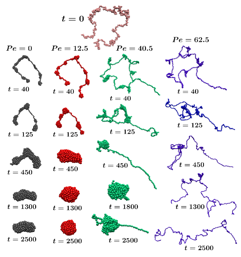
Figure 1: Conformations at different times $t$ (in units of $\sigma^{2}\gamma/\epsilon$) during the evolution of a polymer with $N=380$ for the passive ($Pe=0$) as well as for a few active cases. Snapshot corresponding to $t=0$ represents the starting conformation.

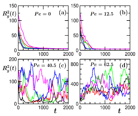
Figure 2: Plots of $R_{g}^{2}$ versus $t$ for a few typical individual runs with $N=380$ for different values of $Pe$ during time evolution of the polymer.

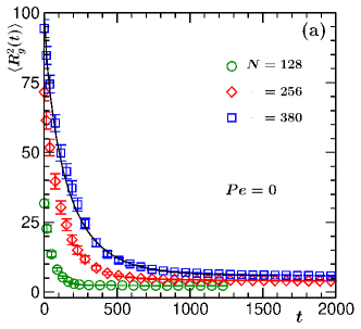
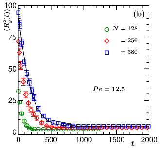
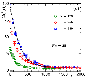
Figure 3: Plots of squared radius of gyration $\langle R_{g}^{2}(t)\rangle$ versus $t$ for (a) the passive case ($Pe=0$) and active chains with (b) $Pe=12.5$ and (c) $Pe=25$, for three different chain lengths.

Coming to active polymers, for low activity strength with $Pe=12.5$, as evident from Fig. 1, the conformations are somewhat similar to those for the passive case. One point to notice is that the final conformation looks somewhat more spherical. Now for $Pe=40.5$ the conformations of the ABPo look quite different than in the earlier cases. The intermediate “pearl-necklace”-like structures do not appear. Instead the polymer makes a “loop-like” structure. Then the end of the polymer where the “loop” has formed, coarsens faster than the other end resulting in a “head-tail”-like conformation. The “head” gradually increases in size by the addition of monomers from the “tail” part and eventually all the monomers become part of a single cluster. Proceeding further in time we observe that the polymer again slowly starts stretching from both the ends. For a much higher activity, with $Pe=62.5$, the conformations at early times look quite similar to the $Pe=40.5$ case. Then with increasing time we see that the polymer stretches more and more instead of collapsing. In this case, the final steady-state conformation of the polymer becomes a completely extended one.

For the quantification of kinetics across the coil-globule transition, we measure the squared radius of gyration defined as

$$R_{g}^{2}=\frac{1}{N}\sum_{i=1}^{N}(\vec{r}_{\rm{cm}}-\vec{r}_{i})^{2},$$ (9)

where $\vec{r}_{\rm{cm}}$ is the center-of-mass of the polymer given by

$$\vec{r}_{\rm{cm}}=\frac{1}{N}\sum_{i=1}^{N}\vec{r}_{i}.$$ (10)

From the average value of $R_{g}^{2}$ it is not possible to understand the fluctuations related to the conformations in each run. As an illustration we show in Figs. 2(a)-(d) the variation of $R_{g}^{2}$ versus $t$ for a few typical runs with $N=380$ at the $Pe$ values used in Fig. 1. For $Pe=0$ and $12.5$, $R_{g}^{2}$ decays monotonically and the individual runs mainly exhibit an up-down shift. Smaller values of $R_{g}^{2}$ close to $5$ for the runs indicate the formation of a globule. For $Pe=40.5$ one observes an oscillatory behavior for any individual run. After reaching a compact globule the structure again starts to extend due to activity of the beads, as seen from Fig. 1. Such oscillatory behavior can not be observed in averaged data as the corresponding times for collapse and re-expansion are not the same for different runs. Now for $Pe=62.5$ the polymer always extends from its starting point. This can be understood by looking at the values of $R_{g}^{2}$ on the $y$-axis.

Next in Fig. 3(a) we plot the average $\langle R_{g}^{2}\rangle$ versus $t$ in the passive case $Pe=0$, for three different values of the chain length. We see that the decay of $R_{g}^{2}$ becomes slower with increasing $N$ as observed earlier Majumder et al. (2017, 2020); Paul et al. (2022). To check for the active cases, in Figs. 3(b) and (c) we plot $\langle R_{g}^{2}\rangle$ versus $t$ for $Pe=12.5$ and $25$, respectively. For these also, we see a similar trend for the decay of $\langle R_{g}^{2}\rangle$ for different $N$ as observed for the passive case.

Table 1: Parameters $b_{0}$, $b_{1}$, $\tau_{c}$, and $\beta$ for different values of $Pe$, obtained by fitting the time dependence of the squared radius of gyration $\langle R_{g}^{2}\rangle$ with the ansatz (11). All data are for $N=380$.

$Pe$	$b_{0}$	$b_{1}$	$\tau_{c}$	$\beta$
0	5.77(9)	94(3)	148(10)	0.78(3)
6.25	4.71(2)	92(2)	119(9)	0.79(3)
12.5	4.59(2)	86(3)	177(10)	1.15(3)
18.75	4.75(2)	85(2)	207(12)	1.28(5)
25	5.03(2)	87(3)	264(19)	1.23(9)
31.25	7.1(7)	90(3)	386(34)	1.09(9)

To have a comparison regarding the relaxation of the ABPo towards its final steady state for different $Pe$, we fit our data with the form Majumder et al. (2017); Paul et al. (2022)

$$\langle R_{g}^{2}(t)\rangle=b_{0}+b_{1}\exp[-(t/\tau_{c})^{\beta}]\,,$$ (11)

where $b_{0}$ is the value of $\langle R_{g}^{2}\rangle$ at $t\to\infty$, i.e., the size of the polymer in its collapsed conformation, $\tau_{c}$ measures the required relaxation time to reach the collapsed state, and $b_{1}$ and $\beta$ are fitting parameters where $b_{1}$ is related to $R_{g}^{2}$ at $t=0$. For $\beta=1$, Eq. (11) corresponds to a purely exponential decay. The solid lines in Figs. 3(a)-(c) for $N=380$ show the resulting fits using the ansatz (11). In Table 1 we quote values of the fitting parameters for a few values of $Pe$. The errors for the fitting parameters are calculated using the Jackknife resampling method Efron (1982). In all cases, the fitted $\beta$ values differ from $1$. For very low activity, i.e., $Pe=6.25$, we see that $\tau_{c}$ is smaller than that for the passive case, indicating a much faster relaxation to the globule. Now with increasing $Pe$ the values of $\tau_{c}$ become larger showing a nonmonotonic behavior of the relaxation time with the variation of $Pe$. Larger error bars for $\tau_{c}$ with $Pe\geq 25$ are due to the presence of larger fluctuations in $R_{g}^{2}$. Interestingly, with increasing $Pe$ one also observes a nonmonotonicity in the values of $b_{0}$ which is related to the size of the globule in its steady state. Larger values of $b_{0}$ indicate that the globules are not completely spherical.

Now we consider the cases with higher activities, i.e., $Pe=40.5$ and $62.5$. As a qualitative comparison among different activities, in Fig. 4(a) we plot $\langle R_{g}^{2}\rangle$ versus time for different $Pe$ values for our longest considered chain, i.e., $N=380$. For $Pe=40.5$ the decay of $\langle R_{g}^{2}\rangle$ is much slower. For much higher activity with $Pe=62.5$, unlike the other cases, $\langle R_{g}^{2}\rangle$ increases from its starting point, reflecting that the steady-state conformation is an extended coil (cf. Fig. 1). Now, we ask whether a stretched conformation of the polymer is a generic feature for a high enough activity. To check for that, in the inset, we plot $\langle R_{g}^{2}\rangle$ versus $t$ for $Pe=62.5$ with two different starting conditions. Along with the data for the extended case similar to the main frame, we also present data for which the starting conformations of the ABPo are globules. Data are presented on a log-log scale to emphasize the differences of the values of $\langle R_{g}^{2}\rangle$ at small $t$. We see that, even after starting from entirely different initial conformations, $\langle R_{g}^{2}\rangle$ for both of them converges towards a similar value at large $t$. It confirms that for high enough $Pe$, when activity dominates over the inter-monomer interactions as well as the thermal fluctuations, the steady-state conformation of the polymer becomes an extended coil.

As another measure of such conformational change due to activity, in Fig. 4(b), we plot the average coordination number $\langle nn\rangle$ of a monomer versus time $t$ for different values of $Pe$ on a log-log scale. $nn$ is calculated by counting the number of beads within the cut-off radius $r_{c}=2.5\sigma$, around a monomer. For passive as well as for lower activities we see that $\langle nn\rangle$ increases with time and saturates for $t\geq 500$. This indicates the formation of a globule. For $Pe=40.5$, $\langle nn\rangle$ also increases but saturates at a smaller value. With higher activity $Pe=62.5$, on the other hand, $\langle nn\rangle$ decreases monotonically which suggests that the polymer becomes extended. As already mentioned, the activity works on each bead along its direction of self-propulsion and thus for very high activities the beads try to move far apart from each other and essentially the polymer becomes elongated.

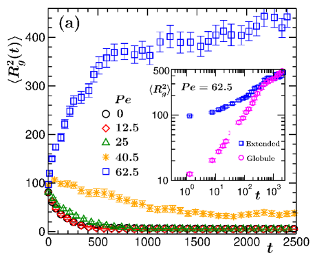
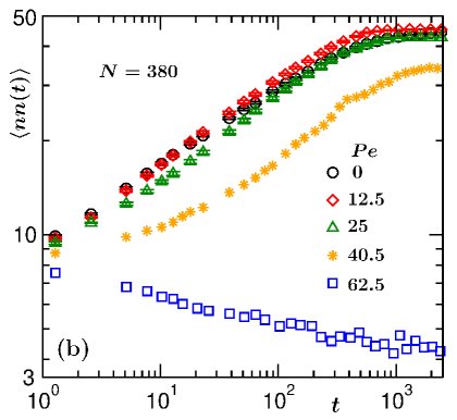
Figure 4: (a) Plot of $\langle R_{g}^{2}(t)\rangle$ versus $t$ for the passive and a few active cases. Inset shows data sets only with $Pe=62.5$, for which different colors mark the cases with starting conformations being extended or a globule one. (b) Log-log plot of the average coordination number $\langle nn\rangle$ of a monomer versus $t$ for the same $Pe$ values as in (a). All data sets are for $N=380$.

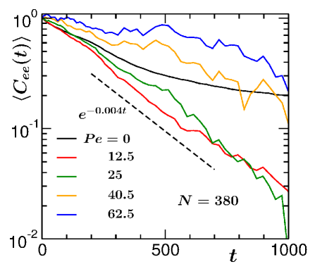
Figure 5: Semi-log plot of the normalized end-to-end vector correlation $\langle C_{ee}(t)\rangle$ versus $t$, on a semi-log scale, for different values of $Pe$. All data are for $N=380$. The dashed line shows an exponential function $\exp(-0.004t)$ as a guide to the eye.

To see the effect of increasing activity on the macroscopic conformational changes with time, we calculated the end-to-end vector correlations and compared them with those for the passive case. This two-time correlation is defined as Eisenstecken et al. (2017)

$$C_{ee}(t)=\vec{r}_{ee}(t)\cdot\vec{r}_{ee}(0)/\vec{r}^{~{}2}_{ee}(0)\,,$$ (12)

where $\vec{r}_{ee}$ stands for the end-to-end vector of the polymer given by

$$\vec{r}_{ee}=\vec{r}_{1}-\vec{r}_{N}\,.$$ (13)

In Fig. 5 we plot this normalized end-to-end vector autocorrelation $\langle C_{ee}(t)\rangle$ versus $t$ on a semi-log scale for the passive as well as for a few active cases. For all of them, starting from a coil conformation, we measure how rapidly the conformations change with time for different values of $Pe$. For lower activities ($Pe=12.5$ and $25$) $\langle C_{ee}(t)\rangle$ follows quite a similar trend as for the passive case until $t\approx 200$. This could be expected from Fig. 1 as the conformations for $Pe=0$ and $12.5$ look visually quite similar. After that initial regime $\langle C_{ee}(t)\rangle$ for $Pe=12.5$ deviates from the passive case and the decay becomes faster. In this regime, the decay is exponential-like and for $200\leq t\leq 700$ data look consistent with $\exp(-0.004t)$. With lower activities, though the final conformations are globules and the decay of $\langle R_{g}^{2}\rangle$ follows a similar trend as that for the passive case, the beads can rearrange themselves within the cluster more rapidly due to their self-propulsion. This certainly helps in modifying the structure of the ABPo and leads to a faster decay of $\langle C_{ee}\rangle$. Now for $Pe=40.5$ the decay of $\langle C_{ee}(t)\rangle$ is always slower compared to the passive and the lower activity cases. This is due to the intermediate conformational changes as observed in Fig. 1. With much higher activity, i.e., for $Pe=62.5$, the decay becomes even slower, as the polymer always remains in the extended state. For the passive case and also for the higher activities it seems like there are continuous changes in the slopes of the decay.

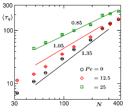
Figure 6: Log-log plot of $\langle\tau_{q}\rangle$, estimated from Eq. (14), versus chain length $N$ for the passive ($Pe=0$) and the active cases with $Pe=12.5$ and $25$. Solid lines represent the power law (15) for which the corresponding exponents are mentioned next to them.

From the previous plots we now have a good comparative picture of the nonequilibrium pathways towards the steady-state conformations of the ABPo for low and high values of $Pe$. Further, we investigate the scaling of the nonequilibrium relaxation time for the collapse. For this, we consider the lower values of $Pe$ for which the final state of the ABPo is a globule. Following earlier works Paul et al. (2022); Majumder et al. (2017), such a characteristic time $\tau_{q}$ can be estimated from the decay of $R_{g}^{2}$ as

$$R_{g}^{2}(t=\tau_{q})=q\Delta R_{g}^{2}+R_{g}^{2}(t\to\infty)\,,$$ (14)

where $R_{g}^{2}(t\to\infty)$ denotes the value of the gyration radius in the globular state and $\Delta R_{g}^{2}=R_{g}^{2}(0)-R_{g}^{2}(t\to\infty)$ measures the total decay. $\tau_{q}$ is the time at which $R_{g}^{2}$ decays to a fraction $q$ of its total decay. This definition is valid for the cases for which $R_{g}^{2}$ decays from its starting value. In our analysis we have taken $q=1/e$. This choice of $q$ is motivated by the exponential-like behavior of the fitting ansatz in Eq. (11) for the data shown in Fig. 3. A more detailed description regarding this can be found in Refs. Paul et al. (2022); Majumder et al. (2020). In Fig. 6 we plot $\langle\tau_{q}\rangle$ versus $N$ for the passive as well as for the active cases with $Pe=12.5$ and $25$. For all the cases, data show power-law behaviors as

$$\langle\tau_{q}\rangle\sim N^{z}\,,$$ (15)

with $z$ as a dynamical exponent Klushin (1998); Majumder et al. (2017, 2020). For the passive polymer case we see $z\simeq 1.35$. Our estimated value for $z$ matches quite well with a few earlier results using Brownian dynamics simulations in absence of hydrodynamics Klushin (1998); Pham et al. (2008); Abrams et al. (2002). However, the dynamics appears to be faster compared to Monte Carlo simulations Majumder et al. (2017, 2020). Now coming to the active cases, with lower activities the exponent $z$ appears to be smaller compared to the passive case. Our estimated values for the exponent $z$ are $\simeq 1.05$ and $\simeq 0.85$, for $Pe=12.5$ and $25$, respectively. This indicates that for lower activities the dynamics of collapse becomes faster than that for the passive case. This scenario is in contrast to the collapse dynamics observed for a polymer with the Vicsek-like alignment activity among the monomers Paul et al. (2022).

III.2 Steady-state properties

Next we investigate the properties of the steady state which is reached once $\langle nn\rangle$ has saturated. In particular we study how the size of the polymer and its related scaling changes with activity. In Fig. 7(a) we plot $\langle R_{g}^{2}\rangle_{s}$ (subscript $s$ indicates steady-state averages) versus $Pe$ over a wide range, for three different chain lengths, i.e., $N=32$, $128$ and $380$, on a semi-log scale. The behavior of $\langle R_{g}^{2}\rangle_{s}$ is indeed representative of a crossover from a globule to extended conformations with increasing $Pe$. For $N=380$, $\langle R_{g}^{2}\rangle_{s}$ first slightly decreases and then increases as a function of $Pe$. A similar nonmonotonic feature can also be identified from the values of the fitting parameter $b_{0}$ in Table 1. From this plot one can identify the corresponding crossover points of $Pe$ which mark the onsets of the change of conformations from globule to the extended state for any $N$. This crossover point $Pe$ increases with $N$. Such a dependence has similarity with the identification of the $\Theta$-transition temperature with the variation of $N$ in the case of a passive polymer Majumder et al. (2017).

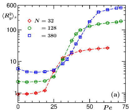
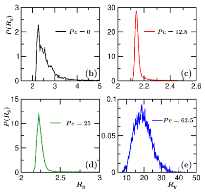
Figure 7: (a) Plot shows the variation of the size of the polymer, $\langle R_{g}^{2}\rangle_{s}$ for its pseudo-equilibrium steady-state conformations, versus $Pe$. (b)-(e) Plots of the normalized distributions of radius of gyration $P(R_{g})$ versus $R_{g}$ for the steady-state conformations at different values of $Pe$ for $N=380$.

For conformational changes of a polymer it is also an usual practice to look at the distribution $P(R_{g})$ of gyration radius for the steady states. In Figs. 7(b)-(e) we plot the normalized $P(R_{g})$ versus $R_{g}$ at different values of $Pe$. There one observes a nonmonotonic behavior regarding the width of the distribution with increasing $Pe$: It decreases for lower activities compared to $Pe=0$ and then increases for higher $Pe$. For passive as well as for lower activities the peaks are at $R_{g}\approx 2.1-2.2$, whereas for $Pe=62.5$ it shifts to the right, i.e., towards a much larger value of $R_{g}\approx 20$. This behavior of $P(R_{g})$ confirms a transition of the polymer from globule to extended state with increasing $Pe$. Similar behavior of $P(R_{g})$ is expected for a passive polymer as well for temperatures below and above its $\Theta$-transition temperature.

Until now we have seen the effect of activity in the macroscopic changes of the polymer. To see the effect in the microscopic details we measure the individual bond lengths $r_{b}$ between any two successive beads, defined as,

$$r_{b}=|\vec{r}_{i+1}-\vec{r}_{i}|\,,$$ (16)

where $\vec{r}_{i}$ represents the position of the $i$-th bead, and looked at their distributions. In Fig. 8 we plot the normalized distributions $P(r_{b})$ for different values of $Pe$ with $N=380$ for the steady-state conformations. We see that the distributions for the lower activities are quite similar to that for the passive case. For much higher activities, i.e., with $Pe=62.5$ and $68.7$ the distributions look very different. They become more asymmetric around their mean. Also the heights of the distributions increase and their widths decrease indicating lesser fluctuations in the variation of $r_{b}$. The shift of the peak positions of $P(r_{b})$ to the right indicates the increase of the average bond length for the conformations. For lower values of $Pe$ the peak occurs around $r_{b}\approx r_{0}=0.7$ whereas for higher $Pe$ the corresponding values of $r_{b}$ appear to be $\approx 0.92$, slightly smaller than the upper limiting value $r_{0}+R=1.0$ of the FENE bonds.

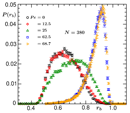
Figure 8: Plots of the normalized distributions of bond lengths $P(r_{b})$ versus $r_{b}$ for different values of $Pe$ for the steady-state conformations.

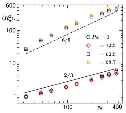
Figure 9: Plots of the steady-state values of the squared gyration radius $\langle R_{g}^{2}\rangle_{s}$ of the polymer versus the chain length $N$ for the passive and a few active cases. The continuous and dashed black lines correspond to power-laws for which the exponents are mentioned next to them.

As observed, the steady state changes from a globular to an extended one with increasing $Pe$. We already got an idea regarding this from Fig. 4(a) which shows that $Pe=62.5$ is high enough for our considered chain lengths here (i.e., up to a maximum of $N=380$) to overcome the attractive forces and to make the conformations more extended. We want to explore further the scaling behavior of $\langle R_{g}^{2}\rangle_{s}$ with $N$. Note that, in absence of self-propulsion of the beads, for the passive polymer this corresponds to an equilibrium state. In this case, the spatial extension of the polymer is related to $N$ via the scaling form Rubinstein and Colby (2003)

$$\langle R_{g}^{2}\rangle_{s}\sim N^{2\nu}\,,$$ (17)

where $\nu$ is known as the Flory exponent. For a passive chain with self-avoidance, the Flory approximation yields for extended coil conformations the value of $\nu=3/(d+2)$, with $d$ being the spatial dimensionality. For $d=3$, $\nu=3/5=0.6$ agrees well with the precise self-avoiding random walk exponent $\nu=0.58759700(40)$ Clisby and Dünweg (2016). On the other hand, $\nu=1/d$, if the conformation of the chain is a globular one. In Fig. 9 we plot $\langle R_{g}^{2}\rangle_{s}$ versus $N$ for a few values of $Pe$. For the passive as well as for lower activity, for which the final conformation is a globule, the exponent is $\nu\approx 1/3$. As expected from Fig. 7(a), for the higher activities, the values of $\langle R_{g}^{2}\rangle_{s}$ are much larger compared to the other cases. For both of them, data look consistent with a power-law behavior with the exponent $\nu\approx 3/5$ similar to that for a self-avoiding random walk. This quantitatively confirms that for higher activities the pseudo-equilibrium steady-state conformations of the polymer are extended coils.

Finally we investigated whether the basis for such a conformational change is embedded in our protocol used for changing the activity. In this regard, we try to understand the relative importance of different energy scales present in the system. For the ABPo, along with the “ballistic” energy $f_{p}\sigma$ and the thermal energy $k_{B}T$, also the interaction energy $\epsilon$ is important. Alongside with $Pe=f_{p}\sigma/k_{B}T$, already defined as the activity parameter, one can define another dimensionless ratio $d_{r}=f_{p}\sigma/\epsilon$. Within the so far employed measurement protocol of changing $f_{p}$ at fixed $T$ and $\epsilon$ (keeping $\sigma$ fixed by default), not only $Pe$ but also $d_{r}$ changes. In Fig. 10 we plot the variation of $d_{r}$ versus $Pe$ while changing $f_{p}$ for fixed values of $\epsilon=1$ and $T=0.1$. $d_{r}$ and $Pe$ are linearly related as

$$d_{r}=\frac{k_{B}T}{\epsilon}Pe\,,$$ (18)

with a slope $k_{B}T/\epsilon=0.1$. The origin with both $d_{r}=Pe=0$ corresponds to the passive polymer case.

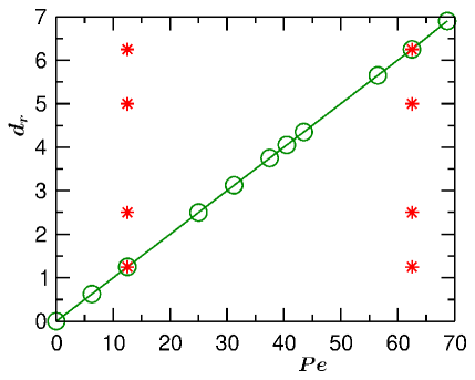
Figure 10: Plot showing the variation of $d_{r}$ versus $Pe$. The line has a slope $k_{B}T/\epsilon=0.1$. The stars mark the corresponding steady-state conformations of the polymer shown in Fig. 11.

In this context, we discuss another possible protocol: If one changes $Pe$ by varying the temperature $T$ for fixed values of $f_{p}$ and $\epsilon$, then $d_{r}$ remains unchanged. In this case one moves along a line parallel to the $Pe$ axis for any fixed $d_{r}$. Thus it is not possible to see the effect of the variation of $d_{r}$ on the polymer conformations. To investigate the effect of increasing $d_{r}$ in such a protocol, we show in Fig. 11 the steady-state conformations for different values of $d_{r}$ for a low and a high value of $Pe$, i.e., $Pe=12.5$ and $62.5$. To perform these simulations we fix $f_{p}=2.0$. Then the temperatures are fixed at $T=0.1$ and $0.02$ to set the $Pe$ values at $12.5$ and $62.5$, respectively. For each of them $d_{r}$ was changed by varying the interaction strength $\epsilon$. For both values of $Pe$, the conformations change from an extended coil to a globule with decreasing $d_{r}$, i.e., increasing $\epsilon$, as observed from Fig. 11. We also checked whether for the high $Pe$ case with small values of $d_{r}$ the globule conformation is generic or not for other combinations of the energy scales. For a higher $f_{p}=10.0$ with $T=0.1$ and $\epsilon=5.0$ (leading also to $Pe=62.5$ and $d_{r}=1.25$) we find that the steady state is also a globule. Now it becomes clearer that $Pe$ is not the only control parameter. Instead, irrespective of the choice of activity strength $f_{p}$, its relative importance compared to the interaction strength $\epsilon$, defined by $d_{r}$, helps in determining the steady-state conformations. Since our way of changing $Pe$ also changes the value of $d_{r}$ we observe the globule to coil transition of ABPo with the variation of $Pe$.

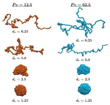
Figure 11: Steady-state conformations of the active polymer with a low ($Pe=12.5$) and a high activity ($Pe=62.5$) for four different values of $d_{r}$ for $N=380$.

IV Conclusion

In this paper, we have studied the kinetics of a flexible polymer consisting of active Brownian beads in a poor solvent. We considered a low enough temperature to minimize the effect of thermal noise on the dynamics of ABPo. The self-propelling force is varied to increase the activity while keeping all other parameters fixed. One sees that with smaller activities, the conformations are qualitatively similar to those for the passive case, and the final conformations are globules. The exponent for the scaling of relaxation time for small $Pe$ becomes lower indicating a faster dynamics for globule formation with increasing $Pe$. However, with much higher activities the conformations become significantly different and the radius of gyration increases with time. This indicates that the polymer becomes more extended.Variation of the gyration radius for the steady-state conformations versus the chain length shows that with increasing activity the corresponding Flory exponent changes from $1/3$ to $3/5$. This indicates a transition of the polymer from a globule to a self-avoiding random walk.

We have understood such a conformational change on the basis of interplay among the three energy scales present in the system. According to our protocol, while changing the self-propelling force $f_{p}$, then along with the variation of the $Pe$ defined as the ratio of the active or “ballistic” energy $f_{p}\sigma$ and the thermal energy $k_{B}T$, another dimensionless ratio $d_{r}=f_{p}\sigma/\epsilon$, where $\epsilon$ is the interaction strength, also changes. Our analyses confirm that the ratio $d_{r}$ plays an important role, driving a change of the steady-state conformation of the ABPo from a globular to the coil state even though the condition is a poor solvent. It will be worthwhile to look at the entire phase diagram for the steady-state conformations in the $Pe$-$d_{r}$ plane. This we intend to investigate in a future work.

Here we considered the Langevin equation in its overdamped limit to mimic the polymer moving in a viscous medium. For active particles one already observed significant differences in the clustering properties when replacing the overdamped Brownian dynamics with the underdamped Langevin equation Löwen (2020). For the active polymer also it can be interesting to look at its properties while the dynamics is mediated via the underdamped Langevin equation which features inertial effects. In our model the ratio of the translational and rotational diffusion constants as well as the self-propulsion force on each bead are chosen as a constant throughout the simulation. But for real systems, in any typical biological environment, the active forces on the beads can have spatial and temporal dependencies as all monomers may not experience the same force at all times. The dependence of particle motility on its local density has already been considered for the Vicsek model Farrell et al. (2012). By taking such a phenomenon into consideration for the ABPo also, this can provide more insights into its typical conformations for real situations. For the ABPo one can also take into account the effect of hydrodynamics which arises due to interaction among the beads and the solvent particles Winkler and Gompper (2020); Martin-Gomez et al. (2020).

V Acknowledgment

This project was funded by the Deutsche Forschungsgemeinschaft (DFG, German Research Foundation) under Grant No. 189 853 844–SFB/TRR 102 (Project B04). It was further supported by the Deutsch-Französische Hochschule (DFH-UFA) through the Doctoral College “$\mathbb{L}^{4}$” under Grant No. CDFA-02-07, the Leipzig Graduate School of Natural Sciences “BuildMoNa”, and the EU COST programme EUTOPIA under Grant No. CA17139.

References

- Chaté et al. (2008) H. Chaté, F. Ginelli, G. Grégoire, F. Peruani, and F. Raynaud, “Modeling collective motion: Variations on the Vicsek model,” Eur. Phys. J. B 64, 451–456 (2008).
- Romanczuk et al. (2012) P. Romanczuk, M. Bär, W. Ebeling, B. Lindner, and L. Schimansky-Geyer, “Active Brownian particles,” Eur. Phys. J. Spec. Top. 202, 1–162 (2012).
- Elgeti et al. (2015) J. Elgeti, R. G. Winkler, and G. Gompper, “Physics of microswimmers—single particle motion and collective behavior: A review,” Rep. Prog. Phys. 78, 056601 (2015).
- Cates and Tailleur (2015) M. E. Cates and J. Tailleur, “Motility-induced phase separation,” Ann. Rev. Cond. Mat. Phys. 6, 219–244 (2015).
- Winkler and Gompper (2020) R. G. Winkler and G. Gompper, “The physics of active polymers and filaments,” J. Chem. Phys. 153, 040901 (2020).
- Shaebani et al. (2020) M. R. Shaebani, A. Wysocki, R. G. Winkler, G. Gompper, and H. Rieger, “Computational models for active matter,” Nat. Rev. Phys. 2, 181–199 (2020).
- Sprenger et al. (2020) A. R. Sprenger, M. A. Fernandez-Rodriguez, L. Alvarez, L. Isa, R. Wittkowski, and H. Löwen, “Active Brownian motion with orientation-dependent motility: Theory and experiments,” Langmuir 36, 7066–7073 (2020).
- Vicsek et al. (1995) T. Vicsek, A. Czirók, E. Ben-Jacob, I. Cohen, and O. Shochet, “Novel Type of Phase Transition in a System of Self-Driven Particles,” Phys. Rev. Lett. 75, 1226–1229 (1995).
- Toner and Tu (1998) J. Toner and Y. Tu, “Flocks, herds, and schools: A quantitative theory of flocking,” Phys. Rev. E 58, 4828–4858 (1998).
- ten Hagen et al. (2011) B. ten Hagen, S. van Teeffelen, and H. Löwen, “Brownian motion of a self-propelled particle,” J. Phys.: Cond. Mat. 23, 194119 (2011).
- Fily and Marchetti (2012) Y. Fily and M. C. Marchetti, “Athermal Phase Separation of Self-Propelled Particles with No Alignment,” Phys. Rev. Lett. 108, 235702 (2012).
- Farrell et al. (2012) F. D. C. Farrell, M. C. Marchetti, D. Marenduzzo, and J. Tailleur, “Pattern formation in self-propelled particles with density-dependent motility,” Phys. Rev. Lett. 108, 248101 (2012).
- McCandlish et al. (2012) S. R. McCandlish, A. Baskaran, and M. F. Hagan, “Spontaneous segregation of self-propelled particles with different motilities,” Soft Matter 8, 2527–2534 (2012).
- Mishra et al. (2012) S. Mishra, K. Tunstrøm, I. D. Couzin, and C. Huepe, “Collective dynamics of self-propelled particles with variable speed,” Phys. Rev. E 86, 011901 (2012).
- Redner et al. (2013) G. S. Redner, M. F. Hagan, and A. Baskaran, “Structure and Dynamics of a Phase-Separating Active Colloidal Fluid,” Phys. Rev. Lett. 110, 055701 (2013).
- Stenhammar et al. (2014) J. Stenhammar, D. Marenduzzo, R. J. Allen, and M. E. Cates, “Phase behaviour of active Brownian particles: The role of dimensionality,” Soft Matter 10, 1489–1499 (2014).
- Das (2017) S. K. Das, “Pattern, growth, and aging in aggregation kinetics of a Vicsek-like active matter model,” J. Chem. Phys. 146, 044902 (2017).
- Siebert et al. (2017) J. T. Siebert, J. Letz, T. Speck, and P. Virnau, “Phase behavior of active Brownian disks, spheres, and dimers,” Soft Matter 13, 1020–1026 (2017).
- Digregorio et al. (2018) P. Digregorio, D. Levis, A. Suma, L. F. Cugliandolo, G. Gonnella, and I. Pagonabarraga, “Full Phase Diagram of Active Brownian Disks: From Melting to Motility-Induced Phase Separation,” Phys. Rev. Lett. 121, 098003 (2018).
- Löwen (2020) H. Löwen, “Inertial effects of self-propelled particles: From active Brownian to active Langevin motion,” J. Chem. Phys. 152, 040901 (2020).
- Paul et al. (2021a) S. Paul, A. Bera, and S. K. Das, “How do clusters in phase-separating active matter systems grow? A study for Vicsek activity in systems undergoing vapor-solid transition,” Soft Matter 17, 645–654 (2021a).
- Deseigne et al. (2012) J. Deseigne, S. Léonard, O. Dauchot, and H. Chaté, “Vibrated polar disks: Spontaneous motion, binary collisions, and collective dynamics,” Soft Matter 8, 5629–5639 (2012).
- Kumar et al. (2014) N. Kumar, H. Soni, S. Ramaswamy, and A. K. Sood, “Flocking at a distance in active granular matter,” Nat. Commun. 5, 1–9 (2014).
- Ravichandran et al. (2017) A. Ravichandran, G. A. Vliegenthart, G. Saggiorato, T. Auth, and G. Gompper, “Enhanced dynamics of confined cytoskeletal filaments driven by asymmetric motors,” Biophys. J. 113, 1121–1132 (2017).
- Lau et al. (2009) A. W. C. Lau, A. Prasad, and Z. Dogic, “Condensation of isolated semi-flexible filaments driven by depletion interactions,” Europhys. Lett. 87, 48006 (2009).
- Vutukuri et al. (2017) H. R. Vutukuri, B. Bet, R. Van Roij, M. Dijkstra, and W. T. S. Huck, “Rational design and dynamics of self-propelled colloidal bead chains: From rotators to flagella,” Sci. Rep. 7, 1–14 (2017).
- Harder et al. (2014) J. Harder, C. Valeriani, and A. Cacciuto, “Activity-induced collapse and reexpansion of rigid polymers,” Phys. Rev. E 90, 062312 (2014).
- Kaiser et al. (2015) A. Kaiser, S. Babel, B. ten Hagen, C. von Ferber, and H. Löwen, “How does a flexible chain of active particles swell?” J. Chem. Phys. 142, 124905 (2015).
- Eisenstecken et al. (2016) T. Eisenstecken, G. Gompper, and R. G. Winkler, “Conformational properties of active semiflexible polymers,” Polymers 8, 304 (2016).
- Isele-Holder et al. (2016) R. E. Isele-Holder, J. Jäger, G. Saggiorato, J. Elgeti, and G. Gompper, “Dynamics of self-propelled filaments pushing a load,” Soft Matter 12, 8495–8505 (2016).
- Eisenstecken et al. (2017) T. Eisenstecken, G. Gompper, and R. G. Winkler, “Internal dynamics of semiflexible polymers with active noise,” J. Chem. Phys. 146, 154903 (2017).
- Duman et al. (2018) Ö. Duman, R. E. Isele-Holder, J. Elgeti, and G. Gompper, “Collective dynamics of self-propelled semiflexible filaments,” Soft Matter 14, 4483–4494 (2018).
- Bianco et al. (2018) V. Bianco, E. Locatelli, and P. Malgaretti, “Globulelike Conformation and Enhanced Diffusion of Active Polymers,” Phys. Rev. Lett. 121, 217802 (2018).
- Paul et al. (2022) S. Paul, S. Majumder, S. K. Das, and W. Janke, “Effects of alignment activity on the collapse kinetics of a flexible polymer,” Soft Matter –, – (2022).
- Paul et al. (2021b) S. Paul, S. Majumder, and W. Janke, “Motion of a polymer globule with Vicsek-like activity: From super-diffusive to ballistic behavior,” Soft Materials 19, 306–315 (2021b).
- Schliwa and Woehlke (2003) M. Schliwa and G. Woehlke, “Molecular motors,” Nature 422, 759–765 (2003).
- Backouche et al. (2006) F. Backouche, L. Haviv, D. Groswasser, and A. Bernheim-Groswasser, “Active gels: Dynamics of patterning and self-organization,” Phys. Biol. 3, 264–273 (2006).
- Jülicher et al. (2007) F. Jülicher, K. Kruse, J. Prost, and J.-F. Joanny, “Active behavior of the cytoskeleton,” Phys. Rep. 449, 3–28 (2007).
- Weber et al. (2015) C. A. Weber, R. Suzuki, V. Schaller, I. S. Aranson, A. R. Bausch, and E. Frey, “Random bursts determine dynamics of active filaments,” Proc. Nat. Acad. Sci. U.S.A. 112, 10703–10707 (2015).
- Suzuki and Bausch (2017) R. Suzuki and A. R Bausch, “The emergence and transient behaviour of collective motion in active filament systems,” Nat. Commun. 8, 1–8 (2017).
- Das et al. (2021) S. Das, N. Kennedy, and A. Cacciuto, “The coil–globule transition in self-avoiding active polymers,” Soft Matter 17, 160–164 (2021).
- Doi and Edwards (1986) M. Doi and S.F. Edwards, The Theory of Polymer Dynamics (Clarendon Press, Oxford, 1986).
- Rubinstein and Colby (2003) M. Rubinstein and R. H. Colby, Polymer Physics (Oxford University Press, New York, 2003).
- Byrne et al. (1995) A. Byrne, P. Kiernan, D. Green, and K. A. Dawson, “Kinetics of homopolymer collapse,” J. Chem. Phys. 102, 573–577 (1995).
- Kuznetsov et al. (1995) Y. A. Kuznetsov, E. G. Timoshenko, and K. A. Dawson, “Kinetics at the collapse transition of homopolymers and random copolymers,” J. Chem. Phys. 103, 4807–4818 (1995).
- Klushin (1998) L. I. Klushin, “Kinetics of a homopolymer collapse: Beyond the Rouse–Zimm scaling,” J. Chem. Phys. 108, 7917–7920 (1998).
- Halperin and Goldbart (2000) A. Halperin and P. M. Goldbart, “Early stages of homopolymer collapse,” Phys. Rev. E 61, 565–573 (2000).
- Abrams et al. (2002) C. F. Abrams, N. K. Lee, and S. P. Obukhov, “Collapse dynamics of a polymer chain: Theory and simulation,” Europhys. Lett. 59, 391–397 (2002).
- Montesi et al. (2004) A. Montesi, M. Pasquali, and F. C. MacKintosh, “Collapse of a semiflexible polymer in poor solvent,” Phys. Rev. E 69, 021916 (2004).
- Kikuchi et al. (2005) N. Kikuchi, J. F. Ryder, C. M. Pooley, and J. M. Yeomans, “Kinetics of the polymer collapse transition: The role of hydrodynamics,” Phys. Rev. E 71, 061804 (2005).
- Pham et al. (2008) T. T. Pham, M. Bajaj, and J. R. Prakash, “Brownian dynamics simulation of polymer collapse in a poor solvent: Influence of implicit hydrodynamic interactions,” Soft Matter 4, 1196–1207 (2008).
- Guo et al. (2011) J. Guo, H. Liang, and Z.-G. Wang, “Coil-to-globule transition by dissipative particle dynamics simulation,” J. Chem. Phys. 134, 244904 (2011).
- Bunin and Kardar (2015) G. Bunin and M. Kardar, “Coalescence Model for Crumpled Globules Formed in Polymer Collapse,” Phys. Rev. Lett. 115, 088303 (2015).
- Majumder et al. (2017) S. Majumder, J. Zierenberg, and W. Janke, “Kinetics of polymer collapse: Effect of temperature on cluster growth and aging,” Soft Matter 13, 1276–1290 (2017).
- Christiansen et al. (2017) H. Christiansen, S. Majumder, and W. Janke, “Coarsening and aging of lattice polymers: Influence of bond fluctuations,” J. Chem. Phys. 147, 094902 (2017).
- Majumder et al. (2020) S. Majumder, H. Christiansen, and W. Janke, “Understanding nonequilibrium scaling laws governing collapse of a polymer,” Eur. Phys. J. B 93, 1–19 (2020).
- Majumder et al. (2019) S. Majumder, U. H. E. Hansmann, and W. Janke, “Pearl-necklace-like local ordering drives polypeptide collapse,” Macromolecules 52, 5491–5498 (2019).
- Jiang and Hou (2014) H. Jiang and Z. Hou, “Motion transition of active filaments: Rotation without hydrodynamic interactions,” Soft Matter 10, 1012–1017 (2014).
- Martin-Gomez et al. (2020) A. Martin-Gomez, T. Eisenstecken, G. Gompper, and R. G. Winkler, “Hydrodynamics of polymers in an active bath,” Phys. Rev. E 101, 052612 (2020).
- Yan et al. (2016) J. Yan, M. Han, J. Zhang, C. Xu, E. Luijten, and S. Granick, “Reconfiguring active particles by electrostatic imbalance,” Nat. Mat. 15, 1095–1099 (2016).
- Daiki et al. (2018) N. Daiki, I. Junichiro, H.-R. Jiang, and M. Sano, “Flagellar dynamics of chains of active Janus particles fueled by an AC electric field,” New J. Phys. 20, 015002 (2018).
- Anand and Singh (2020) S. K. Anand and S. P. Singh, “Conformation and dynamics of a self-avoiding active flexible polymer,” Phys. Rev. E 101, 030501 (2020).
- Milchev et al. (2001) A. Milchev, A. Bhattacharya, and K. Binder, “Formation of block copolymer micelles in solution: A Monte Carlo study of chain length dependence,” Macromolecules 34, 1881–1893 (2001).
- Frenkel and Smit (2002) D. Frenkel and B. Smit, Understanding Molecular Simulation: From Algorithms to Applications (Academic Press, San Diego, 2002).
- Efron (1982) B. Efron, The Jackknife, the Bootstrap and Other Resampling Plans (Society for Industrial and Applied Mathematics, Philadelphia, 1982).
- Clisby and Dünweg (2016) N. Clisby and B. Dünweg, “High-precision estimate of the hydrodynamic radius for self-avoiding walks,” Phys. Rev. E 94, 052102 (2016).