Sample Efficient Grasp Learning Using Equivariant Models

Abstract

In planar grasp detection, the goal is to learn a function from an image of a scene onto a set of feasible grasp poses in $\mathrm{SE}(2)$. In this paper, we recognize that the optimal grasp function is $\mathrm{SE}(2)$-equivariant and can be modeled using an equivariant convolutional neural network. As a result, we are able to significantly improve the sample efficiency of grasp learning, obtaining a good approximation of the grasp function after only 600 grasp attempts. This is few enough that we can learn to grasp completely on a physical robot in about 1.5 hours. Code is available at https://github.com/ZXP-S-works/SE2-equivariant-grasp-learning.

I Introduction

An important trend in robotic grasping is grasp detection where machine learning is used to infer the positions and orientations of good grasps in a scene directly from raw visual input, i.e. raw RGB or depth images. This is in contrast to classical model-based methods that attempt to reconstruct the geometry and pose of objects in a scene and then reason geometrically about how to grasp those objects.

Most current grasp detection models must be trained using large offline datasets. For example, [24] trains on a dataset consisting of over 7M simulated grasps, [2] trains on over 2M simulated grasps, [21] trains on grasp data drawn from over 6.7M simulated point clouds, and [33] trains on over 700k simulated grasps. Some models are trained using datasets obtained via physical robotic grasp interactions. For example, [27] trains on a dataset created by performing 50k grasp attempts over 700 hours, [14] trains on over 580k grasp attempts collected over the course of 800 robot hours, and [1] train on a dataset obtained by performing 27k grasps over 120 hours.

Such high data and time requirements motivate the desire for a more sample efficient grasp detection model, i.e. a model that can achieve good performance with a smaller dataset. In this paper, we propose a novel grasp detection strategy that improves sample efficiency significantly by incorporating equivariant structure into the model. Our key observation is that the target grasp function (from images onto grasp poses) is $\mathrm{SE}(2)$-equivariant. That is, rotations and translations of the input image should correspond to the same rotations and translations of the detected grasp poses at the output of the function. In order to encode the prior knowledge that our target function is $\mathrm{SE}(2)$-equivariant, we constrain the layers of our model to respect this symmetry. Compared with conventional grasp detection models that must be trained using tens of thousands of grasp experiences, the equivariant structure we encode into the model enables us to achieve good grasp performance after only a few hundred grasp attempts.

This paper makes several key contributions. First, we recognize the grasp detection function from images to grasp poses to be $\mathrm{SO}(2)$-equivariant. Then, we propose a neural network model using equivariant layers to encode this property. Finally, we introduce several algorithmic optimizations that enable us to learn to grasp online using a contextual bandit framework. Ultimately, our model is able to learn to grasp well after only approximately 600 grasp trials – 1.5 hours of robot time. Although the model we propose here is only for 2D grasping (i.e. we only detect top down grasps rather than all six dimensions as in 6-DOF grasp detection), the sample efficiency is still impressive and we believe the concepts can be extended to higher-DOF grasp detection models.

These improvements in sample efficiency are important for several reasons. First, since our model can learn to grasp in only a few hundred grasp trials, it can be trained easily on a physical robotic system. This greatly reduces the need to train on large datasets created in simulation, and it therefore reduces our exposure to the risks associated with bridging the sim2real domain gap – we can simply do all our training on physical robotic systems. Second, since we are training on a small dataset, it is much easier to learn on-policy rather than off-policy, i.e. we can train using data generated by the policy being learned rather than with a fixed dataset. This focuses learning on areas of state space explored by the policy and makes the resulting policies more robust in those areas. Finally, since we can learn efficiently from a small number of experiences, our policy has the potential to adapt relatively quickly at run time to physical changes in the robot sensors and actuators.

II Related Work

II-A Equivariant convolutional layers

Equivariant convolutional layers incorporate symmetries into the structure of convolutional layers, allowing them to generalize across a symmetry group automatically. This idea was first introduced as G-Convolution [4] and Steerable CNN [6]. E2CNN is a generic framework for implementing $\mathrm{E}(2)$ Steerable CNN layers [41]. In applications such as dynamics  [36, 40] and reinforcement learning [35, 22, 38, 39] equivariant models demonstrate improvements over traditional approaches.

II-B Sample efficient reinforcement learning

Recent work has shown that data augmentation using random crops and/or shifts can improve the sample efficiency of standard reinforcement learning algorithms [18, 16]. It is possible to improve sample efficiency even further by incorporating contrastive learning [25], e.g. CURL [19]. The contrastive loss enables the model to learn an internal latent representation that is invariant to the type of data augmentation used. The FERM framework [43] applies this idea to robotic manipulation and is able to learn to perform simple manipulation tasks dirctly on physical robotic hardware. The equivariant models used in this paper are similar to data augmentation in that the goal is to leverage problem symmetries to accelerate learning. However, whereas data augmentation and contrastive approaches require the model to learn an invariant or equivariant encoding, the equivariant model layers used in this paper enforce equivariance as a prior encoded in the model. This simplifies the learning task and enables our model to learn faster (see Section V).

II-C Grasp detection

In grasp detection, the robot finds grasp configurations directly from visual or depth data. This is in contrast to classical methods which attempt to reconstruct object or scene geometry and then do grasp planning.

2D Grasping: Several methods are designed to detect grasps in 2D, i.e. to detect the planar position and orientation of grasps in a scene based on top-down images. A key early example of this was DexNet 2.0, which infers the quality of a grasp centered and aligned with an oriented image patch [21]. Subsequent work proposed fully convolutional architectures, thereby enabling the model to quickly infer the pose of all grasps in a (planar) scene [23, 29, 9, 17, 44] (some of these models infer the $z$ coordinate of the grasp as well).

3D Grasping: There is much work in 3D grasp detection, i.e. detecting the full 6-DOF position and orientation of grasps based on TSDF or point cloud input. A key early example of this was GPD [34] which inferred grasp pose based on point cloud input. Subsequent work has focused on improving grasp candidate generation in order to improve efficiency, accuracy, and coverage [24, 32, 13, 10, 2, 1].

On-robot Grasp Learning: Another important trend has been learning to grasp directly from physical robotic grasp experiences. Early examples of this include [27] who learn to grasp from 50k grasp experiences collected over 700 hours of robot time and [20] who learn a grasp policy from 800k grasp experiences collected over two months. QT-Opt [14] learns a grasp policy from 580k grasp experiences collected over 800 hours and [12] extend this work by learning from an additional 28k grasp experiences. [31] learns a grasp detection model from 8k grasp demonstrations collected via demonstration and [42] learns a online pushing/grasping policy from just 2.5k grasps.

III Background

III-A Equivariant Neural Network Models

III-A1 The cyclic group $C_{n}\leq\mathrm{SO}(2)$

In this paper, we are primarily interested in equivariance with respect to the group of planar rotations, $\mathrm{SO}(2)$. However, in practice, in order to make our models computationally tractable, we will use the cyclic subgroup $C_{n}$ of $\mathrm{SO}(2)$, $C_{n}=\{2\pi k/n:0\leq k<n\}$. $C_{n}$ is the group of discrete rotations by multiples of $2\pi/n$ radians.

III-A2 Representation of a group

Elements of the cyclic group $g\in C_{n}$ represent rotations. To specify how these rotations apply to data, we define a representation of the group. However, the type of representation needed depends upon the type of data to be rotated. There are two main representations relevant to this paper. The regular representation acts on an $n$-dimensional vector $(x_{1},x_{2},\dots,x_{n})\in\mathbb{R}^{n}$ by permuting its elements: $\rho_{reg}(g)x=(x_{n-m+1},\dots,x_{n},x_{1},x_{2},\dots,x_{n-m})$ where $g$ is the $m$th element in $C_{n}$. The trivial representation acts on a scalar $x\in\mathbb{R}$ and makes no change at all: $\rho_{0}(g)x=x$. The standard representation $\rho_{1}$ is a rotation matrix that rotates a vector $x$ in the standard way.

III-A3 Feature maps of equivariant convolutional layers

An equivariant convolutional layer maps between feature maps which transform by specified representations $\rho$ of the group. We add an extra channel to the input and output feature maps which encodes the group transformation on feature space. So, whereas the feature map used by a standard convolutional layer is a tensor $\mathcal{F}\in\mathbb{R}^{m\times h\times w}$, an equivariant convolutional layer adds an extra dimension: $\mathcal{F}\in\mathbb{R}^{k\times m\times h\times w}$, where $k$ denotes the dimension of the group representation. This tensor associates each pixel $(x,y)\in\mathbb{R}^{h\times w}$ with a matrix $\mathcal{F}(x,y)\in\mathbb{R}^{k\times m}$.

III-A4 Action of the group operator on the feature map

Given a feature map $\mathcal{F}\in\mathbb{R}^{k\times m\times h\times w}$ associated with group $G$ and representation $\rho$, a group element $g\in G$ acts on $\mathcal{F}$ via:

$$(g\mathcal{F})(x)=\rho(g)\mathcal{F}(\rho_{1}(g)^{-1}x),$$ (1)

where $x\in\mathbb{R}^{2}$ denotes pixel position. In the above, $\rho_{1}(g)^{-1}x$ is the coordinates of pixel rotated by $g^{-1}$ and $\mathcal{F}(\rho_{1}(g)^{-1}x)\in\mathbb{R}^{k\times m}$ is the matrix associated with pixel $\rho_{1}(g)^{-1}x$. The element $g$ operates on $\mathcal{F}(\rho_{1}(g)^{-1}x)$ via the representation $\rho$ associated with the feature map. For example, if $\rho=\rho_{0}$ (the trivial representation), then $k=1$ and $g$ acts on $\mathcal{F}$ by rotating the image but leaving the $m$-vector associated with each pixel unchanged. In contrast, if $\rho=\rho_{reg}$ (the regular representation), then $k=|G|$ (the number of elements in $G$) and $g$ acts on $\mathcal{F}$ by performing a circular shift on the group dimension of $\mathcal{F}(\rho_{1}(g)^{-1}x)$. This last action (by the regular representation) is the one primarily associated with the hidden equivariant convolutional layers used in this paper.

III-A5 The equivariant convolutional layer

An equivariant convolutional layer is a function $h$ from $\mathcal{F}_{in}$ to $\mathcal{F}_{out}$ that is constrained to represent only equivariant functions with respect to a chosen group $G$. The feature maps $\mathcal{F}_{in}$ and $\mathcal{F}_{out}$ are associated with representations $\rho_{in}$ and $\rho_{out}$ acting on feature spaces $\mathbb{R}^{k_{in}}$ and $\mathbb{R}^{k_{out}}$ respectively. Then the equivariant constraint for $h$ is [5]:

$$h(g\mathcal{F}_{in})=gh(\mathcal{F}_{in})=g\mathcal{F}_{out}.$$ (2)

This constraint can be implemented by tying kernel weights $K(y)\in\mathbb{R}^{k_{out}\times k_{in}}$ in such a way as to satisfy the following constraint [5]:

$$K(gy)=\rho_{out}(g)K(y)\rho_{in}(g)^{-1}.$$ (3)

III-B Augmented State Representation (ASR)

We will formulate $\mathrm{SE}(2)$ robotic grasping as the problem of learning a function from an $m$ channel image, $s\in S=\mathbb{R}^{m\times h\times w}$, to a gripper pose $a\in A=\mathrm{SE}(2)$ from which an object may be grasped. Since we will use the contextual bandit framework, we need to be able to represent the $Q$-function, $Q:\mathbb{R}^{m\times h\times w}\times\mathrm{SE}(2)\rightarrow\mathbb{R}$. However, since this is difficult to do using a single neural network, we will use the Augmented State Representation (ASR) [30, 37] to model $Q$ as a pair of functions, $Q_{1}$ and $Q_{2}$.

We factor $\mathrm{SE}(2)=\mathbb{R}^{2}\times\mathrm{SO}(2)$ into a translational component $X\subseteq\mathbb{R}^{2}$ and a rotational component $\Theta\subseteq\mathrm{SO}(2)$. The first function is a mapping $Q_{1}:\mathbb{R}^{m\times h\times w}\times X\rightarrow\mathbb{R}$ which maps from the image $s$ and the translational component of action $X$ onto value. This function is defined to be: $Q_{1}(s,x)=\max_{\theta\in\Theta}Q(s,(x,\theta))$. The second function is a mapping $Q_{2}:\mathbb{R}^{m\times h^{\prime}\times w^{\prime}}\times\Theta\rightarrow\mathbb{R}$ with $h^{\prime}\leq h$ and $w^{\prime}\leq w$ which maps from an image patch and an orientation onto value. This function takes as input a cropped version of $s$ centered on a position $x$, $\mathrm{crop}(s,x)$, and an orientation, $\theta$, and outputs the corresponding $Q$ value: $Q_{2}(\mathrm{crop}(s,x),\theta)=Q(s,(x,\theta))$.

Inference is performed on the model by evaluating $x^{*}=\operatorname*{arg\,max}_{x\in X}Q_{1}(s,x)$ first and then evaluating $Q_{2}(\mathrm{crop}(s,x^{*}),\theta)$. Since each of these two models, $Q_{1}$ and $Q_{2}$, are significantly smaller than $Q$ would be, inference is much faster. Figure 1 shows an illustration of this process. The top of the figure shows the action of $Q_{1}$ while the bottom shows $Q_{2}$. Notice that the semantics of $Q_{2}$ imply that the $\theta$ depends only on $\mathrm{crop}(s,x)$, a local neighborhood of $x$, rather than on the entire scene. This assumption is generally true for grasping because grasp orientation typically depends only on the object geometry near the target grasp point.

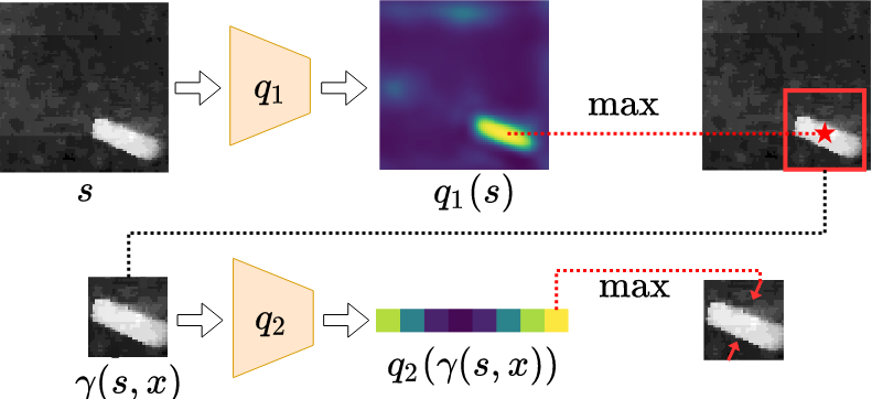
Figure 1: Illustration of the ASR representation. $Q_{1}$ selects the translational component of an action, $Q_{2}$ selects the rotational component.

IV Approach

IV-A Problem Statement

In planar grasp detection, the goal is to estimate a grasp function $\Gamma:\mathbb{R}^{m\times h\times w}\rightarrow\mathrm{SE}(2)$ that maps from a top down image of a scene containing graspable objects, $s\in S=\mathbb{R}^{m\times h\times w}$, to a planar gripper pose, $a\in A=\mathrm{SE}(2)$, from which an object can be grasped. This is similar to the formulations used by [21, 23].

IV-B Formulation as a Contextual Bandit

We formulate grasp learning as a contextual bandit problem where state is the image $s\in S=\mathbb{R}^{m\times h\times w}$ and the action $a\in A=\mathrm{SE}(2)$ is a grasp pose to which the robot hand will be moved and a grasp attempted, expressed in the reference frame of the image. After each grasp attempt, the agent receives a binary reward $R$ drawn from a Bernoulli distribution with unknown probability $r(s,a)$. The true $Q$ function denotes the expected reward of taking action $a$ from $s$. Since $R$ is binary, we have that $Q(s,a)=r(s,a)$. This formulation of grasp learning as a bandit problem is similar to that used by, e.g. [8, 14, 42].

IV-C Invariance Assumption

We assume that the (unknown) reward function $r(s,a)$ that denotes the probability of a successful grasp is invariant to translations and rotations $g\in\mathrm{SE}(2)$. For an image $s\in S=\mathbb{R}^{m\times h\times w}$, let $gs$ denote the the image $s$ translated and rotated by $g$. Similarly, for an action $a\in A=\mathrm{SE}(2)$, let $ga$ denote the action translated and rotated by $g$. Therefore, our assumption is:

$$r(s,a)=r(gs,ga).$$ (4)

Notice that for grasp detection, this assumption is always satisfied because of the way we framed the grasp problem: when the image of a scene transforms, the grasp poses (located with respect to the image) also transform.

IV-D Equivariant Learning

IV-D1 Invariance properties of $Q_{1}$ and $Q_{2}$

Since we have assumed that the reward function $r$ is invariant to transformations $g\in\mathrm{SE}(2)$, the immediate implication is that the optimal $Q$ function is also invariant in the same way, $Q(s,a)=Q(gs,ga)$. In the context of the augmented state representation (ASR, see Section III-B), this implies separate invariance properties for $Q_{1}$ and $Q_{2}$:

$$Q_{1}(gs,gx) =Q_{1}(s,x)$$ (5)

$$Q_{2}(g_{\theta}(\mathrm{crop}(s,x)),g_{\theta}+\theta) =Q_{2}(\mathrm{crop}(s,x),\theta),$$ (6)

where $g_{\theta}\in\mathrm{SO}(2)$ denotes the rotational component of $g\in\mathrm{SE}(2)$, $gx$ denotes the rotated and translated vector $x\in\mathbb{R}^{2}$, and $g_{\theta}(\mathrm{crop}(s,x))$ denotes the cropped image rotated by $g_{\theta}$.

IV-D2 Discrete Approximation of $\mathrm{SE}(2)$

To more practically implement the invariance constraints of Equation 5 and 6 using neural networks, we use a discrete approximation to $\mathrm{SE}(2)$. We constrain the positional component of the action to be a discrete pair of positive integers $x\in\{1\dots h\}\times\{1\dots w\}\subset\mathbb{Z}^{2}$, corresponding to a pixel in $s$, and constrain the rotational component of the action to be an element of the finite cyclic group $C_{n}=\{2\pi k/n:0\leq k<n,i\in\mathbb{Z}\}$. This discretized action space will be written $\hat{\mathrm{SE}}(2)=\mathbb{Z}^{2}\times C_{n}$. (Note that while $\mathbb{Z}^{2}$ and $C_{n}$ are subgroups of $\mathrm{SE}(2)$, the set $\hat{\mathrm{SE}}(2)$ is not; it is just a subsampling of elements from $\mathrm{SE}(2)$.)

IV-D3 Equivariant $Q$-Learning with ASR

In $Q$-Learning with ASR, we approximate $Q_{1}$ and $Q_{2}$ using neural networks. We model $Q_{1}$ as a fully convolutional UNet [28] $q_{1}:\mathbb{R}^{m\times h\times w}\to\mathbb{R}^{1\times h\times w}$ that takes as input the state image and outputs a $Q$-map that assigns each pixel in the input a $Q$ value. We model $Q_{2}$ as a standard convolutional network $q_{2}:\mathbb{R}^{m\times h^{\prime}\times w^{\prime}}\to\mathbb{R}^{n}$ that takes the $h^{\prime}\times w^{\prime}$ image patch as input and outputs an $n$-vector of $Q$ values over $C_{n}$. The networks $q_{1}$ and $q_{2}$ thus represent the functions $Q_{1}$ and $Q_{2}$ by partially evaluating at the first argument and returning a function in the second. As a result, the invariance properties of Equation 5 and 6 for $Q_{1}$ and $Q_{2}$ imply $q_{1}$ and $q_{2}$ are equivariant:

$$q_{1}(gs) =gq_{1}(s)$$ (7)

$$q_{2}(g_{\theta}\mathrm{crop}(s,x)) =\rho_{reg}(g_{\theta})q_{2}(\mathrm{crop}(s,x))$$ (8)

where $g\in\hat{\mathrm{SE}}(2)$ acts on the output of $q_{1}$ through rotating the $Q$-map, and $g_{\theta}\in C_{n}$ acts on the output of $q_{2}$ by performing a circular shift of the output $Q$ values via the regular representation $\rho_{reg}$.

This is illustrated in Figure 2. In Figure 2a we are given the depth image $s$ in the upper left corner. If we rotate this image by $g$ (lower left of Figure 2a) and then evaluate $q_{1}$, we arrive at $q_{1}(gs)$. This corresponds to the LHS of Equation 7. However, because $q_{1}$ is an equivariant function, we can calculate the same result by first evaluating $q_{1}(s)$ and then applying the rotation $g$ (RHS of Equation 7). Figure 2b illustrates the same concept for Equation 8. Here, the network takes the image patch $\mathrm{crop}(s,x)$ as input. If we rotate the image patch by $g_{\theta}$ and then evaluate $q_{2}$, we obtain the LHS of Equation 8, $q_{2}(g_{\theta}\mathrm{crop}(s,x))$. However, because $q_{2}$ is equivariant, we can obtain the same result by evaluating $q_{2}(\mathrm{crop}(s,x))$ and circular shifting the resulting vector to denote the change in orientation by one group element.

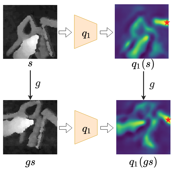
(a) Illustration of Equation 7

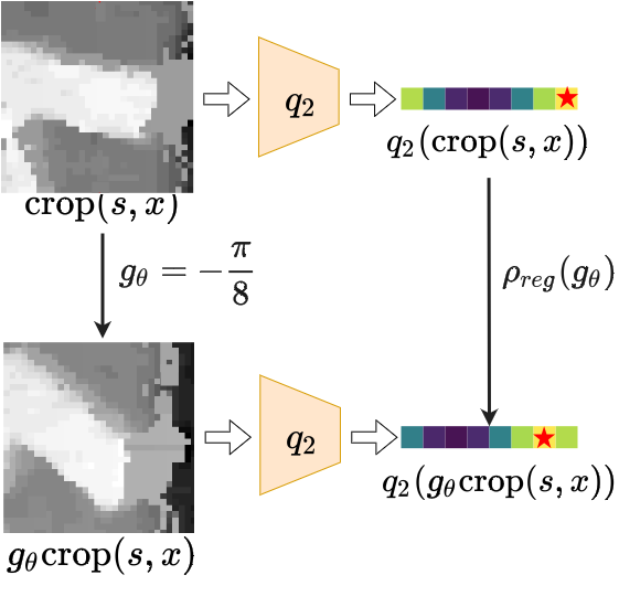
(b) Illustration of Equation 8.

Figure 2: Equivariance relations expressed by Equation 7 and Equation 8.

IV-D4 Model Architecture of Equivariant $q_{1}$

As a fully convolutional network, $q_{1}$ inherits the translational equivariance property of standard convolutional layers. The challenge is to encode rotational equivariance so as to satisfy Equation 7. We accomplish this using equivariant convolutional layers that satisfy the equivariance constraint of Equation 2 where we assign $\mathcal{F}_{in}=s\in{\mathbb{R}^{1\times m\times h\times w}}$ to encode the input state $s$ and $\mathcal{F}_{out}\in\mathbb{R}^{1\times 1\times h\times w}$ to encode the output $Q$ map. Both feature maps are associated with the trivial representation $\rho_{0}$ such that the rotation $g$ operates on these feature maps by rotating pixels without changing their values. We use the regular representation $\rho_{reg}$ for the hidden layers of the network to encode more comprehensive information in the intermediate layers. We found we achieved the best results when we defined $q_{1}$ using the dihedral group $D_{4}$ which expresses the group generated by rotations of multiples of $\pi/2$ in combination with horizontal and vertical reflections.

IV-D5 Model Architecture of Equivariant $q_{2}$

Whereas the equivariance constraint in Equation 7 is over $\hat{\mathrm{SE}}(2)$, the constraint in Equation 8 is over $C_{n}$ only. We implement Equation 8 using Equation 2 with an input of $\mathcal{F}_{in}=\mathrm{crop}(s,x)\in\mathbb{R}^{1\times m\times h^{\prime}\times w^{\prime}}$ as a trivial representation, and an output of $\mathcal{F}_{out}\in\mathbb{R}^{n\times 1\times 1\times 1}$ as a regular representation. $q_{2}$ is defined in terms of the group $C_{n}$, assuming the rotations in the action space are defined to be multiples of $2\pi/n$.

IV-D6 $q_{2}$ Symmetry Expressed as a Quotient Group

It turns out that additional symmetries exist when the gripper has a bilateral symmetry. In particular, it is often the case that rotating a grasp pose by $\pi$ radians about its forward axis does not affect the probability of grasp success, i.e. $r$ is invariant to rotations of the action by $\pi$ radians. When this symmetry is present, we can model it using the quotient group $C_{n}/C_{2}\cong\{2\pi k/n:0\leq k<n/2,k\in\mathbb{Z},0\equiv\pi\}$ which pairs orientations separated by $\pi$ radians into the same equivalence class.

IV-E Other Optimizations

While our use of equivariant models to encode the $Q$ function is responsible for most of our gains in sample efficiency (Section V-C), there are several additional algorithmic details that, taken together, have a meaningful impact on performance.

IV-E1 Loss Function

In the standard ASR loss function, both $q_{1}$ and $q_{2}$ have a Monte Carlo target, i.e. the target is set equal to the transition reward [37]:

$$\mathcal{L} =\mathcal{L}_{1}+\mathcal{L}_{2}$$ (9)

$$\mathcal{L}_{1} =\tfrac{1}{2}(Q_{1}(s,x)-r)^{2}$$ (10)

$$\mathcal{L}_{2} =\tfrac{1}{2}(Q_{2}(\mathrm{crop}(s,x),\theta)-r)^{2}.$$ (11)

However, in order to reduce variance resulting from sparse binary rewards in our bandit formulation, we modify $\mathcal{L}_{1}$:

$$\mathcal{L}_{1}^{\prime}=\frac{1}{2}(Q_{1}(s,x)-(r+(1-r)\max_{\theta\in\bar{\Theta}}\left[Q_{2}(\mathrm{crop}(s,x),\theta)\right]))^{2},$$ (12)

where $\bar{\Theta}=\{\bar{\theta}\neq\theta|\forall\bar{\theta}\in C_{n}/C_{2}\}$. For a positive sample ($r=1$), the $Q_{1}$ target will simply be 1, as it was in Equation 10. However, for a negative sample ($r=0$), we use a TD target calculated by maximizing $Q_{2}$ over $\theta$, but where we exclude the failed $\theta$ action component from $\bar{\Theta}$.

In addition to the above, we add an off-policy loss term $\mathcal{L}_{1}^{\prime\prime}$ that is evaluated with respect to an additional $k$ grasp positions $\bar{X}\subset X$ sampled using a Boltzmann distribution from $q_{1}(s)$:

$$\mathcal{L}_{1}^{\prime\prime}=\frac{1}{k}\sum_{x_{i}\in\bar{X}}\frac{1}{2}\left(Q_{1}(s,x_{i})-\max_{\theta\in\Theta}\left[Q_{2}(\mathrm{crop}(s,x_{i}),\theta)\right]\right)^{2},$$ (13)

where $q_{2}$ provide targets to train $q_{1}$. This off-policy loss minimizes the gap between $q_{1}$ and $q_{2}$. Our combined loss function is therefore $\mathcal{L}=\mathcal{L}_{1}^{\prime}+\mathcal{L}_{1}^{\prime\prime}+\mathcal{L}_{2}$.

IV-E2 Prioritizing failure experiences in minibatch sampling

In the contextual bandit setting, we want to avoid the situation where the agent selects the same incorrect action several times in a row. This can happen because when a grasp fails, the depth image of the scene does not change and therefore the $Q$ map changes very little. We address this problem by ensuring that following a failed grasp experience, that the failed grasp is included in the sampled minibatch on the next SGD step [42], thereby changing the $Q$ function prior to reevaluating it on the next time step. This reduces the chance that the same (bad) action will be selected.

IV-E3 Boltzmann exploration

We compared Boltzmann exploration with $\epsilon$-greedy exploration and found Boltzmann to be better in our grasp setting. We use a temperature of $\tau_{\text{training}}$ during training and a lower temperature of $\tau_{\text{test}}$ during testing. Using a non-zero temperature at test time helped reduce the chances of repeatedly sampling a bad action.

IV-E4 Data augmentation

Even though we are using equivariant neural networks to encode the $Q$ function, it can still be helpful to perform data augmentation as well. This is because the granularity of the rotation group encoded in $q_{1}$ ($D_{4}$) is coarser than that of the action space ($C_{n}/C_{2}$). We address this problem by augmenting the data with translations and rotations sampled from $\hat{\mathrm{SE}}(2)$. For each experienced transition, we add eight additional $\hat{\mathrm{SE}}(2)$-transformed images to the replay buffer.

IV-E5 Softmax at the output of $q_{1}$ and $q_{2}$

Since we are using a contextual bandit with binary rewards and the reward function $r(s,a)$ denotes the parameter of a Bernoulli distribution at $s,a$, we know that $Q_{1}$ and $Q_{2}$ must each take values between zero and one. We encode this prior using an entry-wise softmax layer at the output of each of the $q_{1}$ and $q_{2}$ networks.

IV-E6 Selection of the $z$ coordinate

In order to execute a grasp, we must calculate a full $x,y,z$ goal position for the gripper. Since our model only infers a planar grasp pose, we must calculate a depth along the axis orthogonal to this plane (the $z$ axis) using other means. In this paper, we calculate $z$ by taking the average depth over a $5\times 5$ pixel region centered on the grasp point in the input depth image. The commanded gripper height is set to an offset value from this calculated height. While executing the motion to this height, we monitor force feedback from the arm and halt the motion prematurely if a threshold is exceeded. (In our physical experiments on the UR5, this force is measured using torque feedback from the joints.)

V Experiments in Simulation

V-A Setup

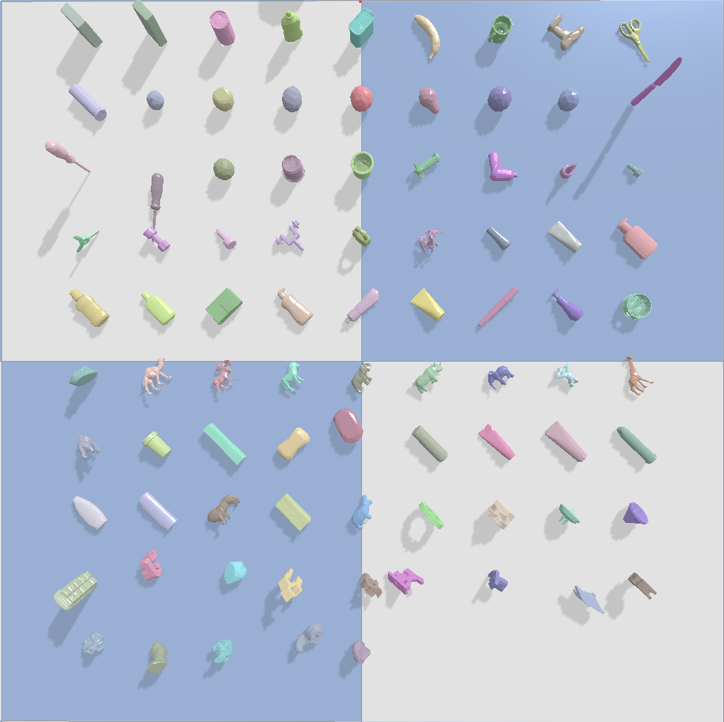
(a) 86 GraspNet-1B objects used

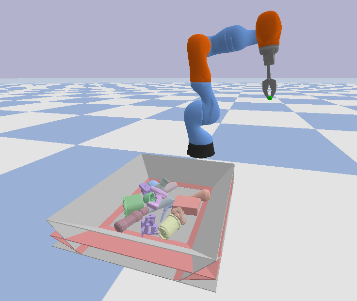
(b) Pybullet simulation

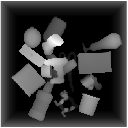
(c) Depth image

Figure 3: (a) The 86 objects used in our simulation experiments drawn from the GraspNet-1Billion dataset [10]. (b) Phybullet simulation. (c) State is a top-down image of the grasp scene.

V-A1 Object Set

All simulation experiments are performed using objects drawn from the GraspNet-1Billion dataset [10]. This includes 32 objects from the YCB dataset [3], 13 adversarial objects used in DexNet 2.0 [21], and 43 additional objects unique to GraspNet-1Billion [10] (a total of 88 objects). Out of these 88 objects, we exclude two bowels because they can be stably placed in non-graspable orientations, i.e. they can be placed upside down and cannot be grasped in that orientation using standard grippers. Also, we scale these objects so that they are graspable from any stable object configuration. we refer to these 86 mesh models as our simulation “object set”, shown in Figure 3a.

V-A2 Simulation Details

Our experiments are performed in Pybullet [7]. The environment includes a Kuka robot arm and a $0.3\text{m}\times 0.3\text{m}$ tray with inclined walls (Figure 3b). At the beginning of each episode, the environment is initialized with $15$ objects drawn uniformly at random from our object set and dropped into the tray from a height of $40$ cm so that they fall into a random configuration. State is a depth image captured from a top-down camera (Figure 3c). On each time step, the agent perceives state and selects an action to execute which specifies the planar pose to which to move the gripper. A grasp is considered to have been successful if the robot is able to lift the object more than $0.1$m above the table. The episode continues until all objects have been removed from the tray or until $30$ grasp attempts have been made at which point the episode terminates and the environment is reinitialized.

V-B Comparison Against Baselines

V-B1 Baseline Model Architectures

We compare our method against two different model architectures from the literature: VPG [42] and FC-GQ-CNN [29]. Each model is evaluated alone and then with two different data augmentation strategies (soft equ and RAD). In all cases, we use the contextual bandit formulation described in Section IV-B. The baseline model architectures are: VPG: Architecture used for grasping in [42]. This model is a fully convolutional network (FCN) with a single-channel output. The $Q$ value of different gripper orientations is evaluated by rotating the input image. We ignore the pushing functionality of VPG. FC-GQ-CNN: Model architecture used in [29]. This is an FCN with $8$-channel output that associates each grasp rotation to a channel of the output. During training, our model uses Boltzmann exploration with a temperature of $\tau=0.01$ while the baselines use $\epsilon$-greedy exploration starting with $\epsilon=50\%$ and ending with $\epsilon=10\%$ over 500 grasps (this follows the original implementation in [42]).

V-B2 Data Augmentation Strategies

The data augmentation strategies are: $n\times$ RAD: The method from [18] where we perform $n$ SGD steps after each grasp sample, where each SGD step is taken over a mini-batch of samples for which the observation and action have been randomly translated and rotated. $n\times$ soft equ: same as $n\times$ RAD except that we produce a mini-batch by drawing $bs/n$ (where $bs$ is the batch size) samples and then randomly augmenting those samples $n$ times. Details can be found in Appendix -C.

V-B3 Results

The learning curves of Figure 4 show grasp success rate versus number of grasp attempts. Figure 4a shows on-line learning performance. Our method uses Boltzmann exploration while the baselines use $\epsilon$-greedy as described above. Each curve connects data points evaluated every 150 grasp attempts. Each data point is the average success rate over the last 150 grasps (therefore, the first data point occurs at 150). Figure 4b shows near-greedy performance by stopping training every 150 grasp attempts and performing 1000 test grasps and reporting average performance over these 1000 test grasps. Our method tests at a lower test temperature of $\tau=0.002$ while the baselines test pure greedy behavior.

V-B4 Discussion of Results

Generally, our proposed equivariant model convincingly outperforms the baseline methods and data augmentation strategies. In particular, Figure 4b shows that the grasp success rate of the near-greedy policy learned by the equivariant model after 150 grasp attempts is at least as good as that learned by any of the other baselines methods after 1500 grasp attempts. Notice that each of the two data augmentation methods we consider (RAD and soft equ) have a positive effect on the baseline methods. However, after training for the full 1500 grasp attempts, our equivariant model converges to the highest grasp success rate ($93.9\pm 0.4\%$).

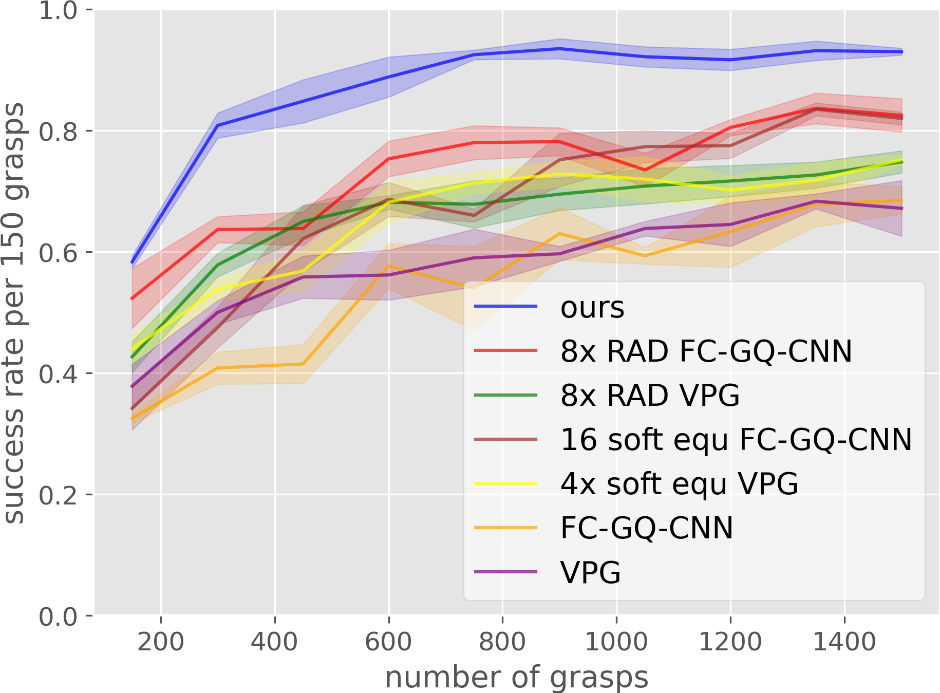
(a) Training

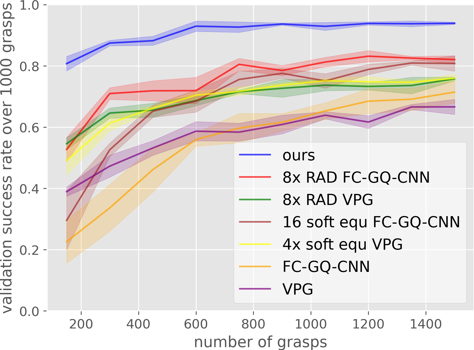
(b) Testing

Figure 4: Comparison with baselines. All lines are an average of four runs. Shading denotes standard error. (a) shows learning curves as a running average over the last 150 training grasps. (b) shows average near-greedy performance of 1000 validation grasps performed every 150 training steps.

V-C Ablation Study

There are three main parts to the approach described in this paper: 1) use of equivarant convolutional layers instead of standard convolution layers; 2) use of the augmentated state representation (ASR) instead of a single network; 3) the various optimizations described in Section IV-E. Here, we evaluate performance of the method when ablating each of these three parts.

V-C1 Ablations

In no equ, we replace all equivariant layers with standard convolutional layers. In no ASR, we replace the equivariant $q_{1}$ and $q_{2}$ models described in Section III-B by a single equivariant network. In no opt, we remove the optimizations described in Section IV-E. In addition to the above, we also evaluated rot equ which is the same as no ASR except that we replace ASR with a U-net[28] and apply $4\times$ RAD[18] augmentation. Detailed network architectures can be found in Appendix -A.

V-C2 Results and Discussion

Figure 5 shows the results where they are reported exactly in the same manner as in Section V-B. no equ does worst, suggesting that our equivariant model is critical. We can improve on this somewhat by adding data augmentation (rot equ), but this sill underperforms significantly. The other ablations, no ASR and no opt demonstrate that those parts to the method are also important.

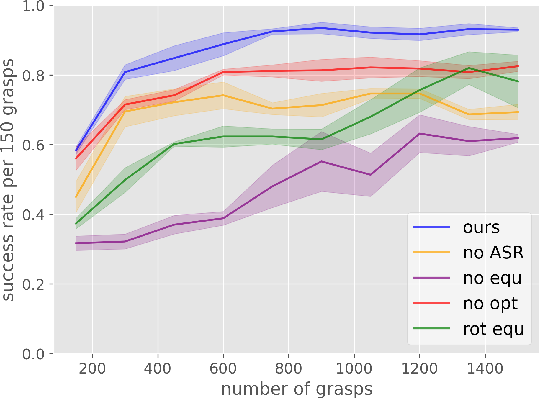
(a) Training

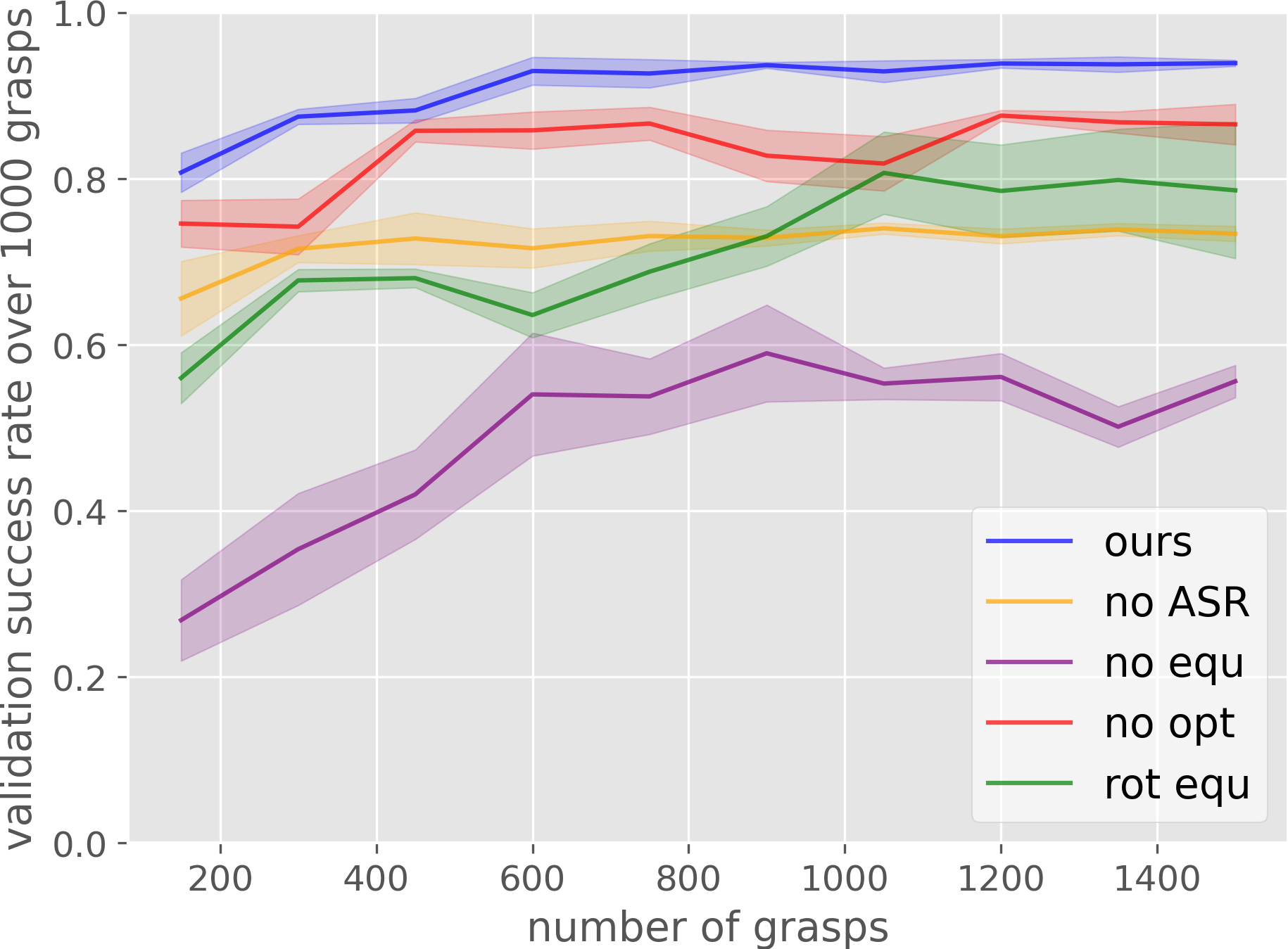
(b) Testing

Figure 5: Ablation study. Lines are an average over $4$ runs. Shading denotes standard error. (a) learning curves as a running average over the last 150 training grasps. (b) average near-greedy performance of 1000 validation grasps performed every 150 training steps.

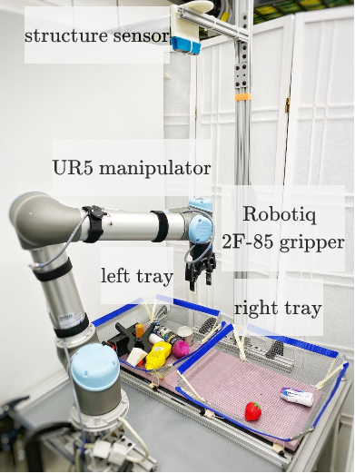
Figure 6: Setup for self-supervised training on the robot.

VI Experiments in Hardware

VI-A Setup

VI-A1 Robot Environment

Our experimental platform is comprised of a Universal Robots UR5 manipulator equipped with a Robotiq 2F-85 parallel-jaw gripper, an Occipital Structure Sensor, and the dual-tray grasping environment shown in Figure 6. The work station is equipped with Intel Core i7-7800X CPU and NVIDIA GeForce GTX 1080 GPU.

VI-A2 Objects

All training happens using the 15 objects shown in Figure 8a. After training, we evaluate grasp performance on both the “easy” test objects (Figure 8b) and the “hard” test objects (Figure 8c). Note that both test sets are novel with respect to the training set.

VI-A3 Self-Supervised Training

At the beginning of training, the 15 training objects (Figure 8a) are dropped into one of the two trays by the human operator. Then, we train by attempting to grasp these objects and place them in the other bin. All grasp attempts are generated by the contextual bandit. When all 15 objects have been transported in this way, training switches to attempting to grasp from the other bin and transport them into the first. Training continues in this way until 600 grasp attempts have been performed (that is 600 grasp attempts, not 600 successful grasps). A grasp is considered to be successful if the gripper remains open after closing stops due to a squeezing force. To avoid systematic bias in the way the robot drops objects into a tray, we sample the drop position randomly from a Gaussian distribution centered in the middle of the receiving tray.

VI-A4 In-Motion Computation

We were able to nearly double the speed of robot training by doing all image processing and model learning while the robotic arm was in motion. This was implemented in Python as a producer-consumer process using mutexs. As a result, our robot is constantly in motion during training and the training speed for our equivariant algorithm is completely determined by the speed of robot motion. This improvement enabled us to increase robot training speed from approximately 230 grasps per hour to roughly 400 grasps per hour.

VI-A5 Model Details

For all methods, prior to training on the robot, model weights are initialized randomly using an independent seed. No experiences from simulation are used, i.e. we train from scratch. The model and training parameters used in the robot experiments are the same as those used in simulation. For our algorithm, the $q_{1}$ network is defined using $D_{4}$-equivariant layers and the $q_{2}$ network is defined using $C_{16}/C_{2}$-equivariant layers. During training, we use Boltzmann exploration with a temperature of $0.01$. During testing, the temperature is reduced to $0.002$ (near-greedy). For more details, see Appendix -F.

Baseline	test set easy	test set hard	training $t_{\text{SGD}}$
$8\times$ RAD VPG	61.8 $\pm$3.59	52.5 $\pm$5.33	12.1
$8\times$ RAD FC-GQ-CNN	82.8 $\pm$1.65	74.3 $\pm$3.04	1.55
Ours	95.0 $\pm$1.47	87.0 $\pm$1.87	1.11

TABLE I: Evaluation success rate ($\%$), standard error, and training time per grasp (in seconds) in the hardware experiments. Results are an average of 100 grasps per training run averaged over four runs, performed on the held out test objects shown in Figure 8b and c.

VI-A6 Baselines

In our robot experiments, we compare our method against $8\times$ RAD VPG [42] [18] and $8\times$ RAD FC-GQ-CNN [29] [18], the two baselines we found to perform best in simulation. As before, $8\times$ RAD VPG, uses a fully convolutional network (FCN) with a single output channel. The $Q$ map for each gripper orientation is calculated by rotating the input image. After each grasp, we perform $8\times$ RAD data augmentation (8 optimization steps with a mini-batch containing randomly translated and rotated image data). $8\times$ RAD FC-GQ-CNN also has an FCN backbone, but with eight output channels corresponding to each gripper orientation. It uses $8\times$ RAD data augmentation as well. All exploration is the same as it was in simulation except that the $\epsilon$-greedy schedule goes from $50\%$ to $10\%$ over 200 steps rather than over 500 steps.

VI-A7 Evaluation procedure

A key failure mode during testing is repeated grasp failures due to an inability of the model to learn quickly enough. To combat this, we use the procedure of [42] to reduce the chances of repeated grasp failures (we use this procedure only during testing, not training). After a grasp failure, we perform multiple SGD steps using that experience to “discourage” the model from selecting the same action a second time and then use that updated model for the subsequent grasp. Then, after a successful grasp has occurred, we discard these updates and return to the original network.

VI-B Results

VI-B1 Results

Figure 7 shows the learning curves for the three methods during learning. Each curve is an average of four runs starting with different random seeds and random object placement. Each data point is the average grasp success over the last 60 grasp attempts during training. Table I shows the performance of all methods after the 600-grasp training is complete. All methods are evaluated by freezing the corresponding model and executing 100 greedy (or near greedy) test grasps for the easy-object test set (Figure 8b) and 100 additional test grasps for the hard-object test set (Figure 8c).

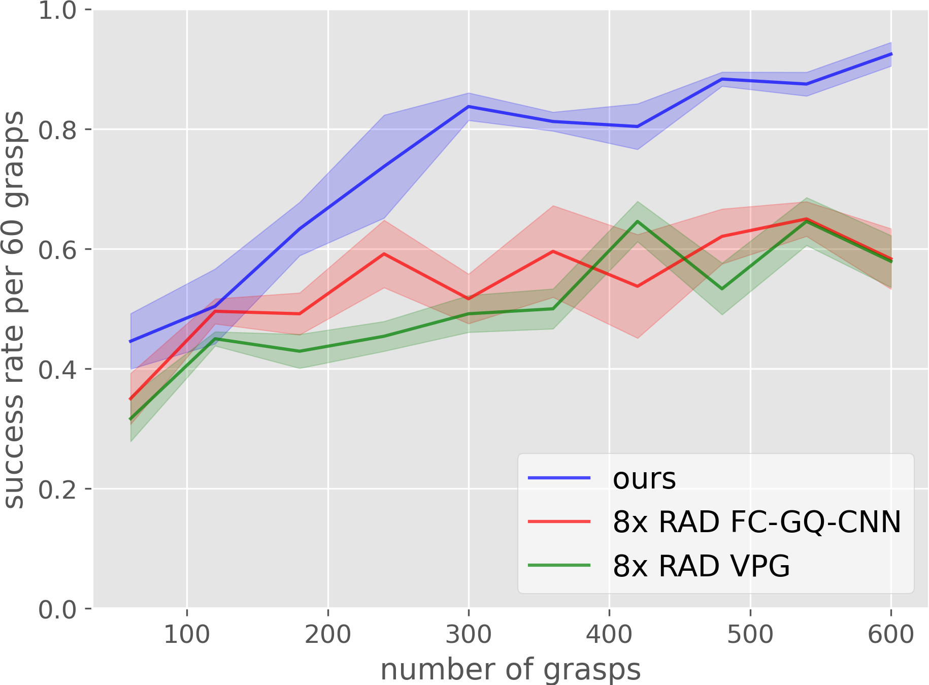
Figure 7: Learning curves for the hardware experiment. All curves are averaged over $4$ runs. Shading denotes standard error.

VI-B2 Discussion

Probably the most important observation to make is that the results from training on the physical robot (Figure 7) matches the simulation training results (Figure 4a) closely. After 600 grasp attempts, our method achieves a success rate of $>90\%$ while the baselines are near $70\%$. The other observation is that since each of these 600-grasp training runs takes approximately 1.5 hours, it is reasonable to expect that this method could adapt to physical changes in the robot very quickly. Looking at Table I, our method significantly outperforms the baselines during testing as well, although performance is significantly lower on the “hard” test set. We hypothesize that the lower “hard” set performance is due to a lack of sufficient diversity in the training set.

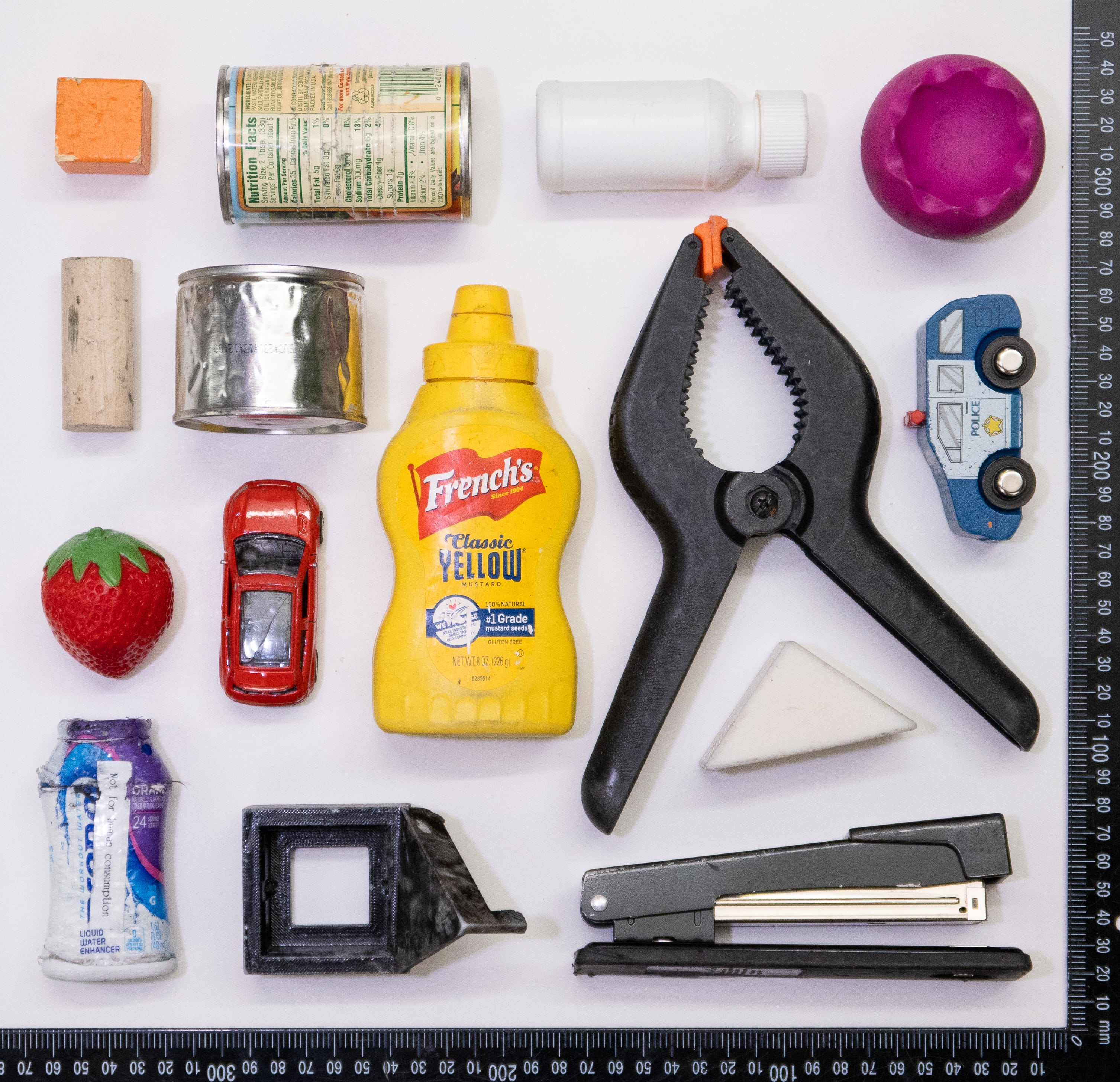
(a) Training set

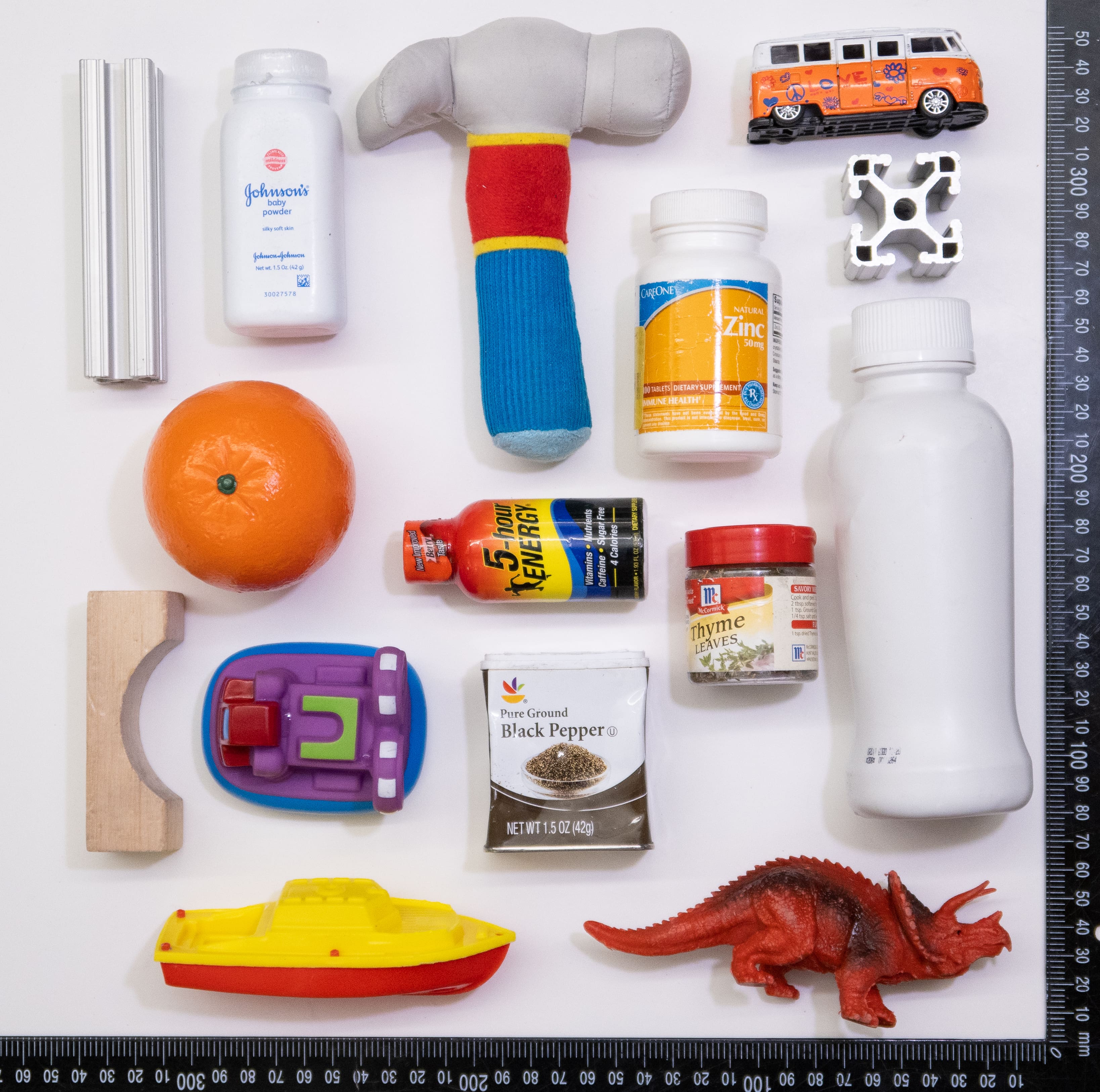
(b) Testing set, easy

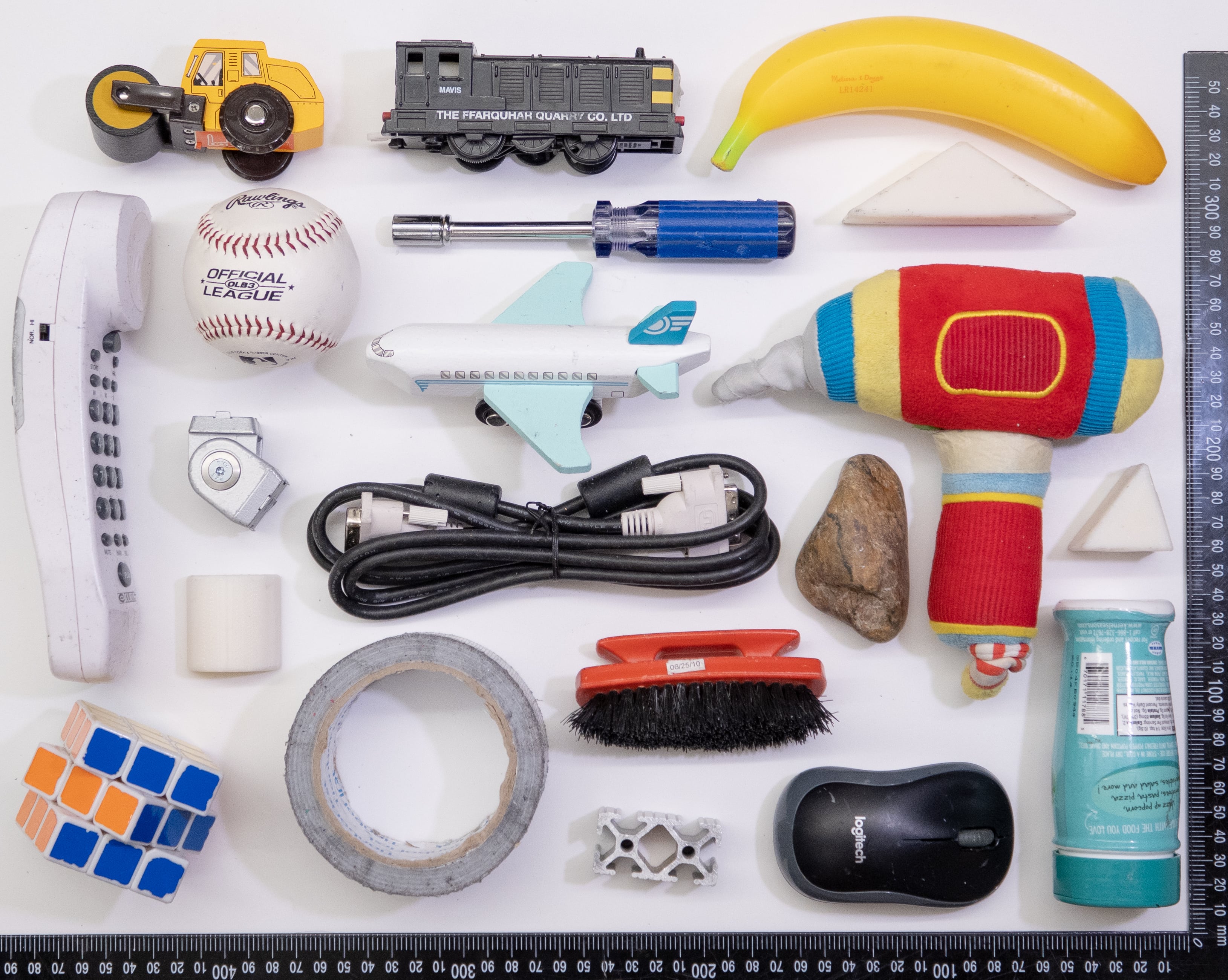
(c) Testing set, hard

Figure 8: Object sets used for training and testing. Both training and test set easy include 15 objects while test set hard has 20 objects. Objects were curated so that they were graspable by the Robotiq 2F-85 parallel jaw gripper from any configuration and visible to the Occipital Structure Sensor.

VII Experiments with the Jacquard Dataset

We also evaluated our model using a large online dataset known as Jacquard [9] consisting of approximately 54k RGBD images with a total of 1.1M labeled grasps [9].

VII-1 Setup

Here, we discard the bandit framework and simply evaluate our equivariant model on Jacquard in the context of supervised learning. Since our focus is on sample efficiency, we train our model on small randomly sampled subsets of 16, 64, 256, and 1024 images drawn randomly from the 54k Jacquard images. In all cases, we evaluated against a single set of 240 Jacquard images held out from all training images. We preprocess the Jacquard images by rectifying the image background in the depth channel so that it is parallel to the image plane.

VII-2 Baselines

We evaluate our model against the following baselines: GG-CNN [23]: a generative grasping fully convolutional network (FCN) that predicts grasp quality, angle, and width; GR-Conv-Net [17]: similar to GG-CNN, but it incorporates a generative residual FCN; VPG [42]: an FCN with a single-channel output – the model architecture used in VPG. The $Q$-value of different gripper orientations is evaluated by rotating the input image; FC-GQ-CNN [29]: an FCN with 16 channel output that associates each grasp rotation to a channel of the output. Since both GG-CNN and GR-Conv-Net were originally designed for the supervised learning setting, we use those methods as originally proposed. However, since VPG, FC-GQ-CNN, and our method are on-policy, we discard the on-policy aspects of those methods and just retain the model. For those methods that output discrete grasp angles, we discretize the grasp angle into 16 orientations between 0 and $\pi$ radians and 16 different values for gripper width.

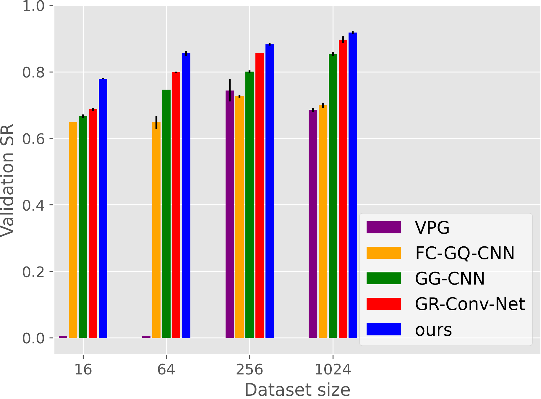
Figure 9: Grasp success rates on Jacquard dataset. All models were trained with four datasets sized 16, 64, 256, and 1024 images. Error bar denotes standard deviation. Results averaged over two runs with independent seeds.

VII-3 Results

Figure 9 evaluates the grasp success rates for our method in comparison with the baselines. As is standard in Jaquard, a grasp is considered a “success” when the IOU is greater than 25% and the predicted grasp angle is within 30 degrees of a ground truth grasp. The horizontal axis of Figure 9 shows success rates for the various methods as a function of the four training set sizes. Our proposed equivariant method outperforms in all cases.

VIII Conclusions and Limitations

This paper recognises that planar grasp detection where the input is an image of the scene and the output is a planar grasp pose is $\mathrm{SE}(2)$-equivariant. We propose using an $\mathrm{SO}(2)$-equivariant model architecture to encode this structure. The resulting method is significantly more sample efficient than other grasp learning approaches and can learn a good grasp function in less than 600 grasp samples. A key advantage of this increase in sample efficiency is that we are able to learn to grasp completely on the physical robotic system without any pretraining in simulation. This increase in sample efficiency could be important in robotics for a couple of reasons. First, it obviates the need for training in simulation (at least for some problems like grasping), thereby making the sim2real gap less of a concern. Second, it opens up the possibility for our system to adapt to idiosyncrasies of the robot hardware or the physical environment that are hard to simulate. A key limitation of these results, both in simulation and on the physical robot, is that despite the fast learning rate, grasp success rates (after training) still seems to be limited to the low/mid $90\%$ range. This is the same success rate seen in with other grasp detection methods [21, 34, 24], but it is disappointment here because one might expect faster adaptation to lead ultimately to better grasp performance. This could simply be an indication of the complexity of the grasp function to be learned or it could be a result of stochasticity in the simulator and on the real robot.

-A Neural network architecture

Our network architecture is shown in Figure 10a. The $q1$ network is a fully convolutional UNet [28]. The $q2$ network is a residual neural network [11]. These networks are implemented using PyTorch [26], and the equivariant networks are implemented using the E2CNN library [41]. Adam optimizer [15] is used for the SGD step. The ablation no opt has the same architecture as above. The ablation no asr (Figure 10b) ablated the $q2$ network and is defined with respect to group $C16$. The ablation no equ (Figure 10c) has a similar network architecture as ours with approximately the same number of free weights. However, the equivariant network is replaced with an FCN. The ablation rot equ (Figure 10d) has a similar network architecture as no asr method with approximately the same number of free weights. However, the equivariant network is replaced with an FCN.

-B Parameter choices

The parameters we choose in simulation (Section V-A) and in hardware (Section VI) are listed in tables II, III, and IV.

TABLE II: Parameter choices for all methods.

environment	parameter	value
in simulation, in hardware	$bs$ batch size	8 (2 for VPG)
	number of rotations	8
	augment buffer	$8$ times
	augment buffer type	random $\mathrm{SE}(2)$, flip
	$d_{\text{dilation}}$	4 pixels
in simulation	$s_{\text{threshold}}$	0.5cm
	workspace size	$0.3\times 0.3$m
	state $s$ size	$128^{2}$ pixel
	action range	$96^{2}$ pixel
in hardware	$s_{\text{threshold}}$	1.5cm
	workspace size	$0.25\times 0.25$m
	state $s$ size	$112^{2}$ pixel
	action range	$80^{2}$ pixel

TABLE III: Parameter choices for ours.

environment	parameter	value
in simulation, in hardware	train SGD step after	the 20th grasp
	policy	Boltzmann
	$crop(s,x)$ size	32
	learning rate	1e-4
	weight decay	1e-5
	$k$ in $L_{1}^{{}^{\prime\prime}}$	10
	$\tau$ in $L_{1}^{{}^{\prime\prime}}$	1
	$\tau_{\text{test}}$	0.01
	$\tau_{\text{train}}$	0.002
	SGD step per grasps	1

TABLE IV: Parameter choices for baselines.

environment	parameter	value
in simulation, in hardware	train SGD step after	the 1st grasp
	policy	$\epsilon$-greedy
	$\epsilon_{\text{initial}}$	0.5
	$\epsilon_{\text{final}}$	0.1
	$\epsilon$ linear schedule	200 grasps in simulation
		500 grasps in hardware

-C Augmentation baseline choices

The data augmentation strategies are: $n\times$ RAD: The method from [18] where we perform $n$ SGD steps after each grasp sample, where each SGD step is taken over a mini-batch $bs$ of samples that have been randomly translated and rotated by $g\in\hat{\mathrm{SE}}(2)$. $n\times$ soft equ: a data augmentation method [38] that performs $n$ soft equivariant SGD steps per grasp, where each SGD step is taken over $n$ times randomly $\hat{\mathrm{SE}}(2)$ augmented mini-batch. Specifically, we sample $bs/n$ samples ($bs$ is the batch size), augment it $n$ times and train on this mini-batch. We perform this SGD steps $n$ times so that $bs$ transitions are sampled. This augmentation aims at achieving equivariance in the mini-batch.

We apply $n\times$ RAD and $n\times$ soft equ data augmentation to both VPG and FC-GQ-CNN baselines, with $n={2,4,8}$. Figure 11 shows the results. Observe that all data augmentation choices improve the baselines, but an increase in $n$ leads to a saturation effect in learning while causing more computation overhead. The best data augmentation parameters $n$ are chosen for each baseline in the comparison in Figure 4

For rot equ ablation baseline, we choose the best learning curve in Figure 12b, i.e, $4\times$ RAD rot FCN. This baseline aims to achieve equivariance through the combination of data augmentation and rotation encoding of an FCN.

(a) ours and no opt

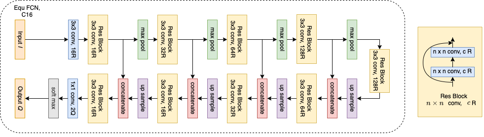
(b) no asr

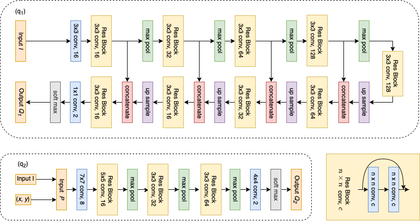
(c) no equ

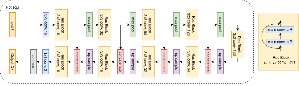
(d) Rot equ

Figure 10: The neural network architecture for ours and ablations. R means regular representation, T means trivial representation, Q means quotient representation.

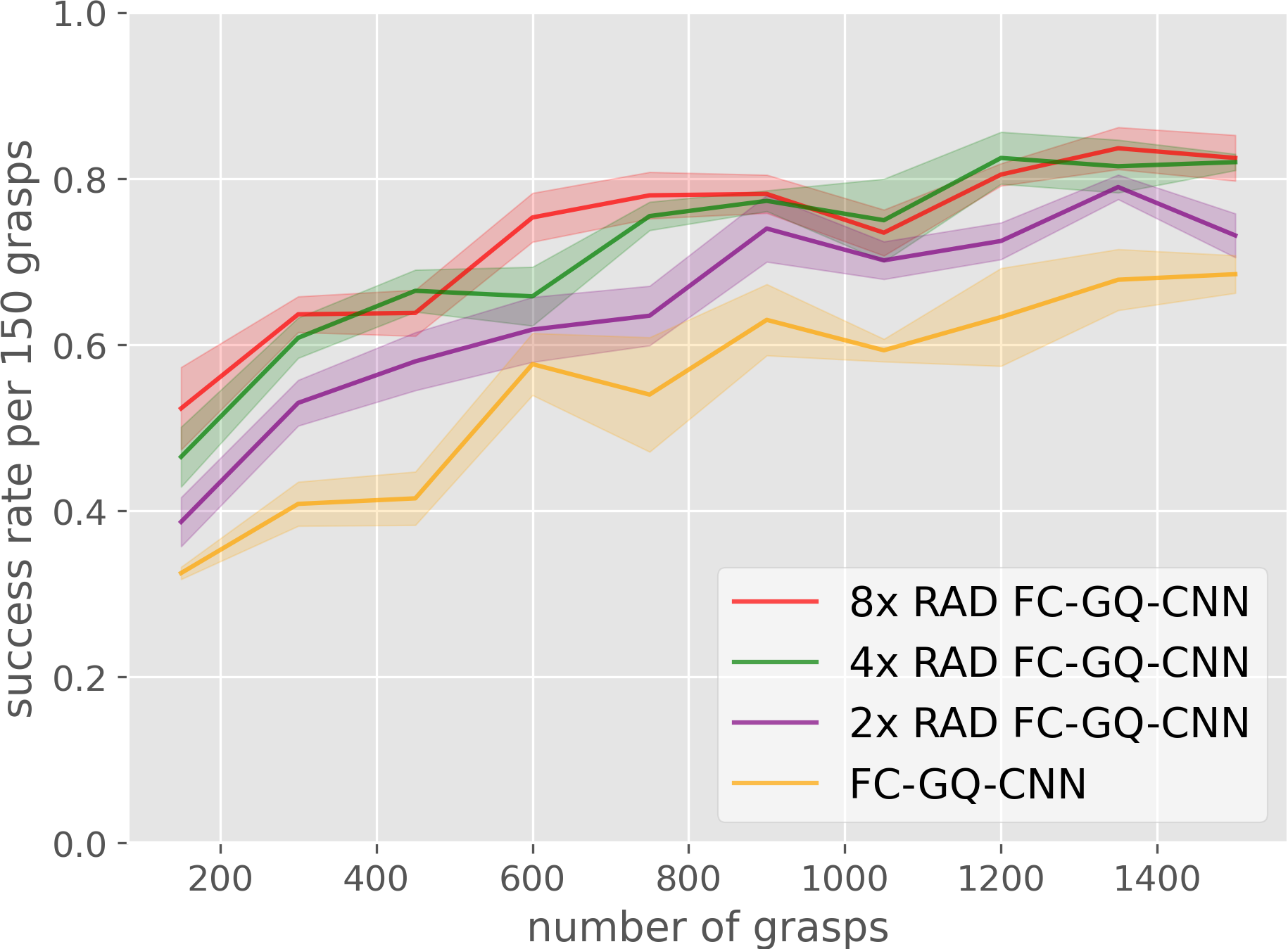
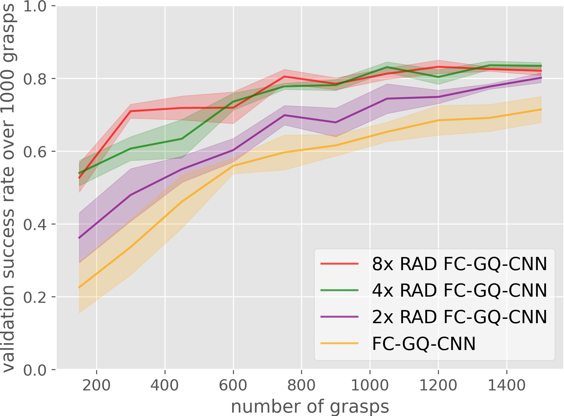
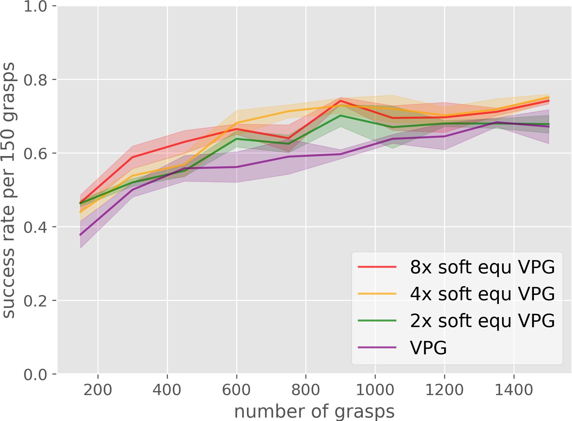
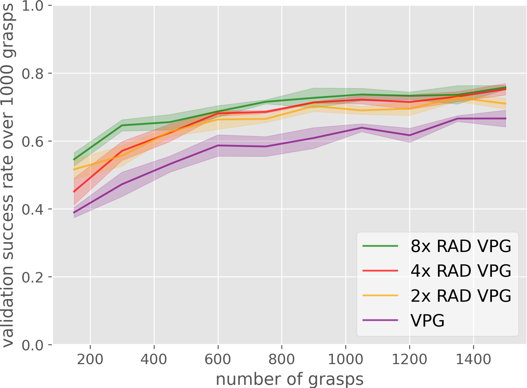
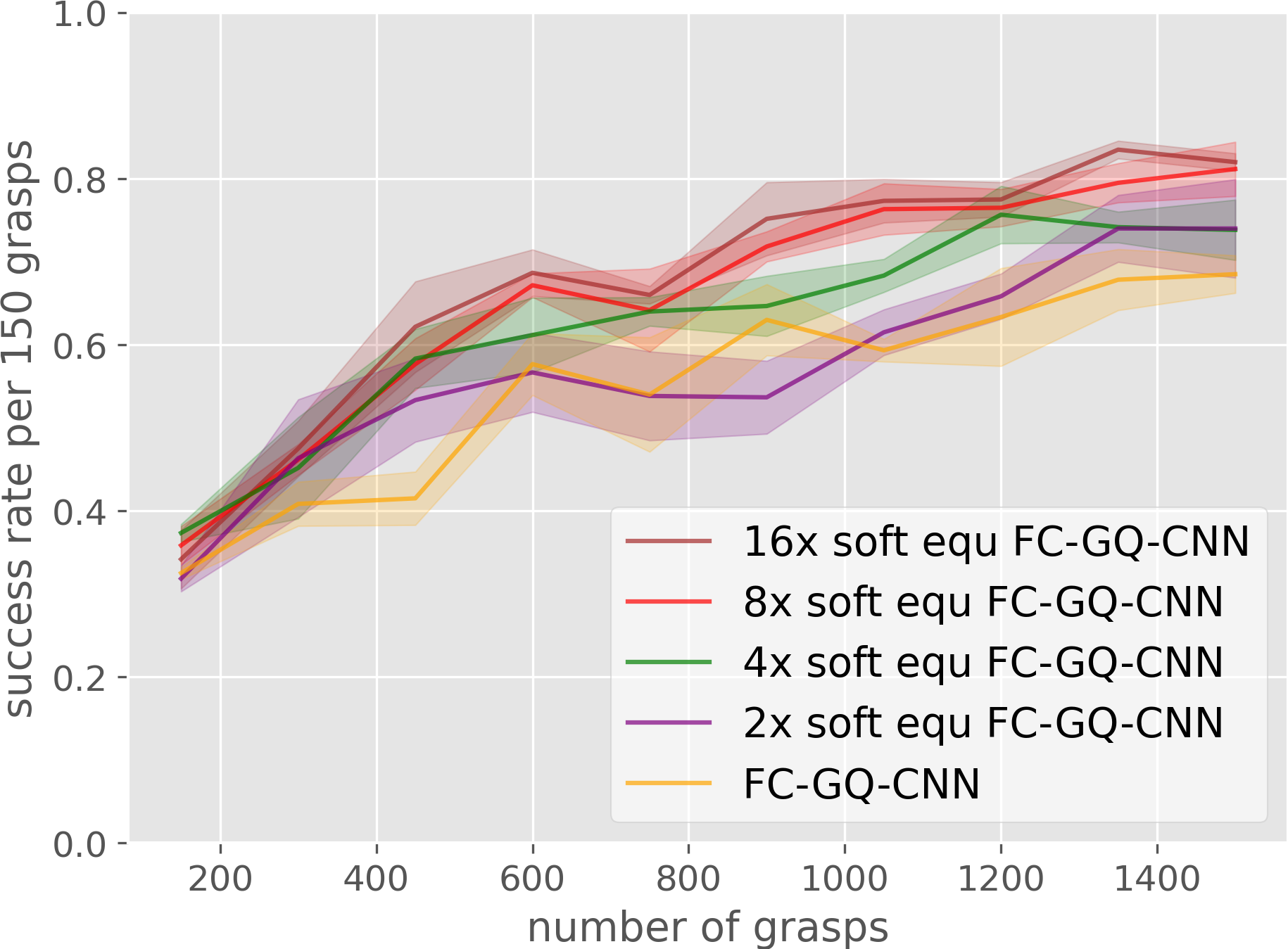
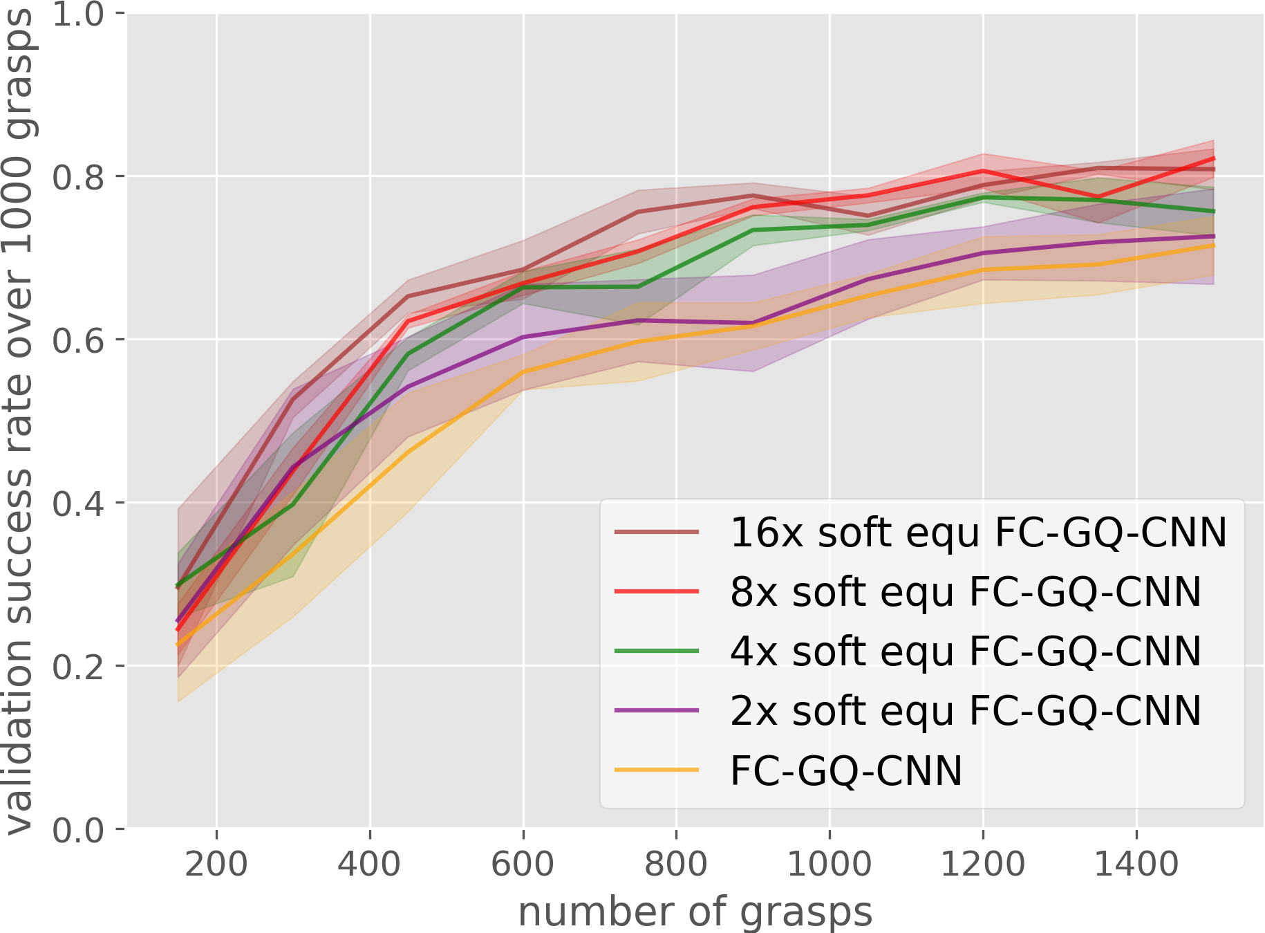
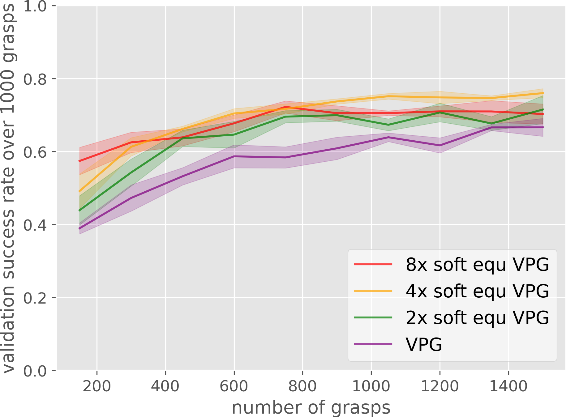
Figure 11: Baseline with data augmentation. The first two columns are FC-GQ-CNN while the last two columns are VPG. The first row is $n\times$ RAD augmentation whereas the last row is $n\times$ soft equ augmentation. The baselines without augmentation prefix are the baselines without augmentation.

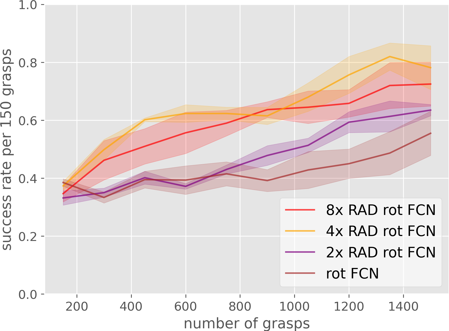
(a) Training

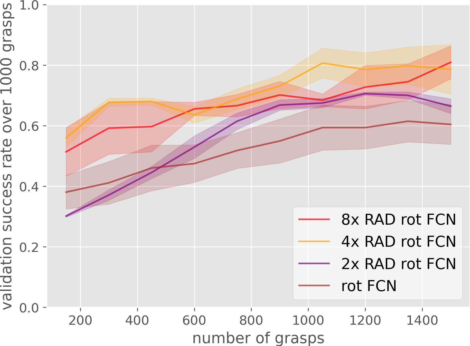
(b) Testing

Figure 12: Baseline comparisons for Rot equ. We refer rot equ as the best learning curve in (b), i.e, $4\times$ RAD rot FCN.

-D Success and failure modes

We list typical success and failure modes to evaluate our algorithm’s performance.

For success modes, the learned policy of our method showcases its intelligence. At the densely cluttered scene, our method prefers to grasp the relatively isolated part of the objects, see Figure 14a, b. At the scene where the objects are close to each other, our method can find the grasp pose that doesn’t cause a collision/interference with other objects, see Figure 14c, d.

For failure modes, we identify several typical scenarios: Wrong action selection (Figure 15a, b, and e) indicates that there is a clear gap between our method and optimal policy, this might be caused by the biased dataset collected by the algorithm. Reasonable grasps failure (Figure 15d, f) means that the agent selects a reasonable grasp, but it fails due to the stochasticity of the real world, i.e., sensor noise, contact dynamics, hardware flaws, etc. Challenging scenes (Figure 15c, g) is the nature of densely cluttered objects, it can be alleviated by learning an optimal policy or executing higher DoFs grasps. The sensor distortion (Figure 15h) is caused by an imperfect sensor. Among all failure modes, wrong action selection takes the most part (65% failure in the test set easy and 33% failure in the test set hard). It is followed by reasonable grasps, challenging scenes, and then sensor distortion.

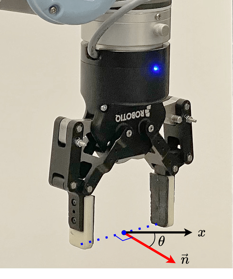
Figure 13: The definition of $\theta$. $x$ is the $x$-axle of the workspace while $\vec{n}$ is the normal of the gripper.

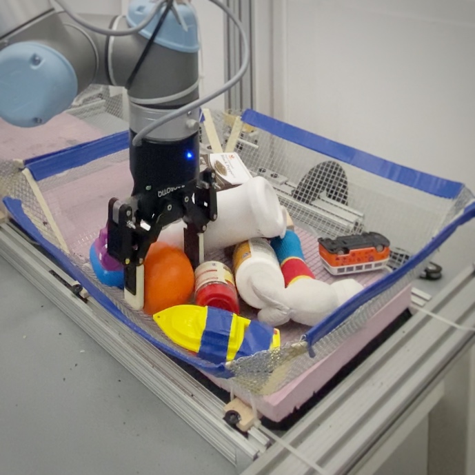
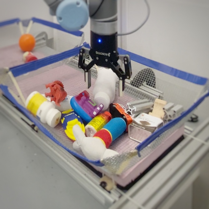
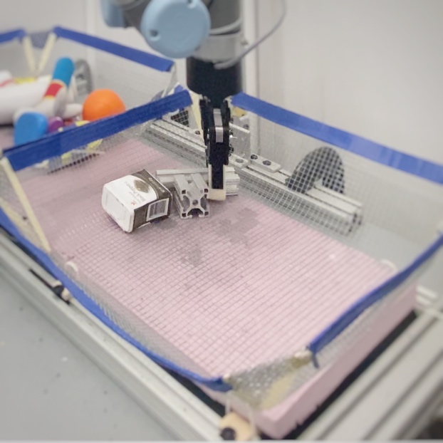
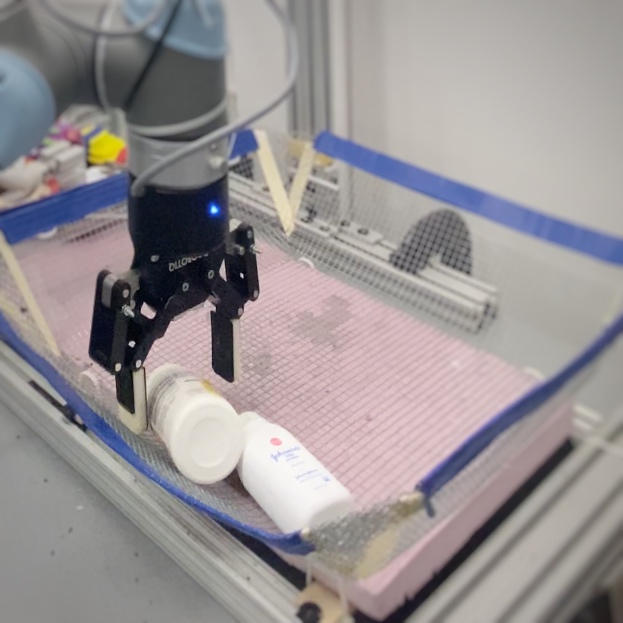
Figure 14: Success modes in the test set easy, which has 15 hold out objects.

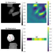
(a) Wrong $q_{1}$ (10/20)

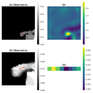
(b) Wrong $q_{2}$ (3/20)

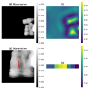
(c) Challenging scenes (3/20)

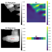
(d) Reasonable grasps (3/20)

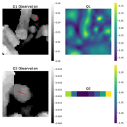
(e) Wrong $q_{1}$ (17/52)

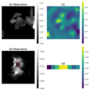
(f) Reasonable grasps (13/52)

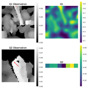
(g) Challenging scenes (11/52)

(h) Sensor distortion (8/52)

Figure 15: Failure modes. The brackets show the failure times divided by the total number of failures in all four runs. The first row is test in the test set easy while the second row is test in the test set hard.

-E Action space details

The action $\theta$ is defined as the angle between the normal vector $\vec{n}$ of the gripper and the $x$-axle, see Figure 13.

To prevent the grasps in the empty space where there is no object in $s$, we constrain the action space to $x_{\text{positive}}\in X$ to exclude the empty space, see Figure 16c. The constrain $x_{\text{positive}}$ is achieved by first thresholding the depth image: $s_{\text{positive}}=s>s_{\text{threshold}}$ ($s_{\text{threshold}}$ is 0.5cm in simulation and 1.5cm in hardware), then dilate this binary map $s_{\text{positive}}$ by radius $d_{\text{dilation}}=4$ pixels. The parameter $s_{\text{threshold}}$ is selected according to sensor noise where $d_{\text{dilation}}$ is related to the half of the gripper aperture. Moreover, we constrain the action space within the tray to prevent collision.

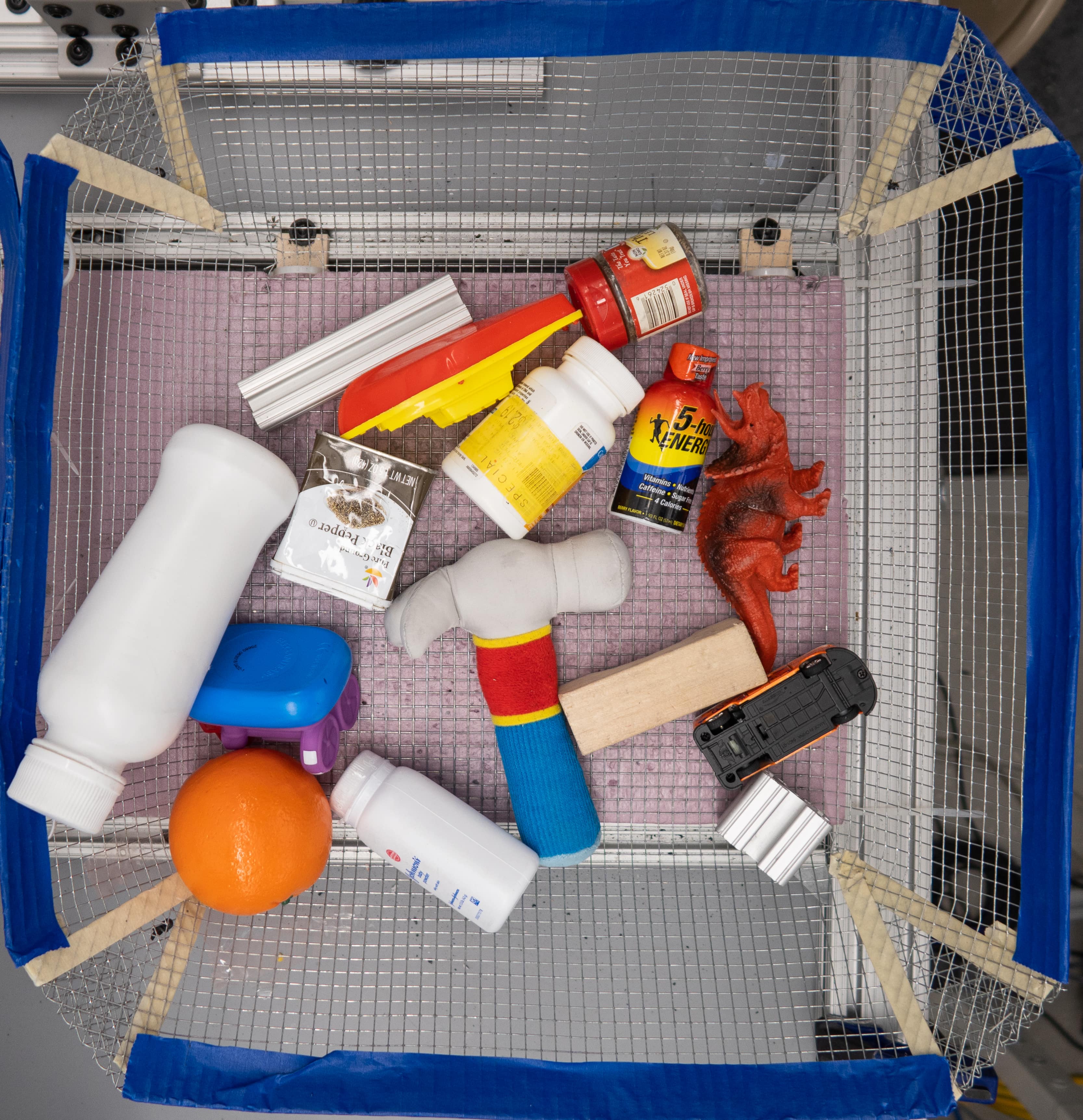
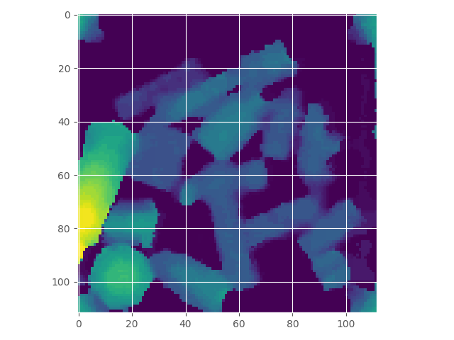
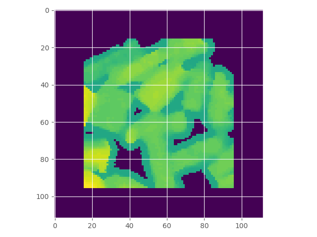
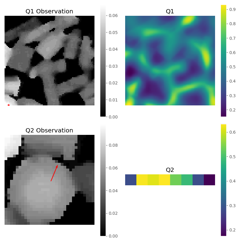
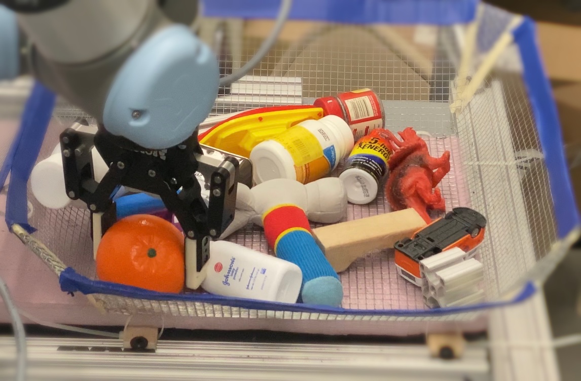
Figure 16: Action space constraint for action selection. (a) Test set easy cluttered scene. (b) The state $s$. (c) The action space $x_{\text{positive}}$, it overlays the binary mask $x_{\text{positive}}$ with the state $s$ for visualization. (d) The $Q$-values within the action space. (e) Selecting an action. (f) Executing a grasp.

-F Evaluation details in hardware

The evaluation policy and environment are different from that of training in the following aspects. First, for all methods, the robot arm moves slower than that during training in the environment. This helps form stable grasps. Second, for our method, the evaluation policy uses a lower temperature ($\tau_{\text{test}}=0.002$) than training. After a failure grasp, ours performs $2$ SGD steps on this failure experience. The network weight will be reloaded after recovery from the failure [42]. For the baselines, the evaluation policy uses a greedy policy. After a failure grasp, baselines perform $8$ RAD SGD steps on this failure experience. The network weight will be reloaded after recovery from the failure [42].

References

- Berscheid et al. [2021] Lars Berscheid, Christian Friedrich, and Torsten Kröger. Robot learning of 6 dof grasping using model-based adaptive primitives. arXiv preprint arXiv:2103.12810, 2021.
- Breyer et al. [2021] Michel Breyer, Jen Jen Chung, Lionel Ott, Roland Siegwart, and Juan Nieto. Volumetric grasping network: Real-time 6 dof grasp detection in clutter. arXiv preprint arXiv:2101.01132, 2021.
- Calli et al. [2017] Berk Calli, Arjun Singh, James Bruce, Aaron Walsman, Kurt Konolige, Siddhartha Srinivasa, Pieter Abbeel, and Aaron M Dollar. Yale-cmu-berkeley dataset for robotic manipulation research. The International Journal of Robotics Research, 36(3):261–268, 2017. doi: 10.1177/0278364917700714. URL https://doi.org/10.1177/0278364917700714.
- Cohen and Welling [2016a] Taco Cohen and Max Welling. Group equivariant convolutional networks. In International conference on machine learning, pages 2990–2999. PMLR, 2016a.
- Cohen et al. [2018] Taco Cohen, Mario Geiger, and Maurice Weiler. A general theory of equivariant cnns on homogeneous spaces. arXiv preprint arXiv:1811.02017, 2018.
- Cohen and Welling [2016b] Taco S Cohen and Max Welling. Steerable cnns. arXiv preprint arXiv:1612.08498, 2016b.
- Coumans and Bai [2016] Erwin Coumans and Yunfei Bai. Pybullet, a python module for physics simulation for games, robotics and machine learning. GitHub repository, 2016.
- Danielczuk et al. [2020] Michael Danielczuk, Ashwin Balakrishna, Daniel S Brown, Shivin Devgon, and Ken Goldberg. Exploratory grasping: Asymptotically optimal algorithms for grasping challenging polyhedral objects. arXiv preprint arXiv:2011.05632, 2020.
- Depierre et al. [2018] Amaury Depierre, Emmanuel Dellandréa, and Liming Chen. Jacquard: A large scale dataset for robotic grasp detection. CoRR, abs/1803.11469, 2018. URL http://arxiv.org/abs/1803.11469.
- Fang et al. [2020] Hao-Shu Fang, Chenxi Wang, Minghao Gou, and Cewu Lu. Graspnet-1billion: A large-scale benchmark for general object grasping. In Proceedings of the IEEE/CVF Conference on Computer Vision and Pattern Recognition, pages 11444–11453, 2020.
- He et al. [2015] Kaiming He, Xiangyu Zhang, Shaoqing Ren, and Jian Sun. Deep residual learning for image recognition, 2015.
- James et al. [2019] Stephen James, Paul Wohlhart, Mrinal Kalakrishnan, Dmitry Kalashnikov, Alex Irpan, Julian Ibarz, Sergey Levine, Raia Hadsell, and Konstantinos Bousmalis. Sim-to-real via sim-to-sim: Data-efficient robotic grasping via randomized-to-canonical adaptation networks. In Proceedings of the IEEE/CVF Conference on Computer Vision and Pattern Recognition, pages 12627–12637, 2019.
- Jiang et al. [2021] Zhenyu Jiang, Yifeng Zhu, Maxwell Svetlik, Kuan Fang, and Yuke Zhu. Synergies between affordance and geometry: 6-dof grasp detection via implicit representations. arXiv preprint arXiv:2104.01542, 2021.
- Kalashnikov et al. [2018] Dmitry Kalashnikov, Alex Irpan, Peter Pastor, Julian Ibarz, Alexander Herzog, Eric Jang, Deirdre Quillen, Ethan Holly, Mrinal Kalakrishnan, Vincent Vanhoucke, and Sergey Levine. Qt-opt: Scalable deep reinforcement learning for vision-based robotic manipulation. CoRR, abs/1806.10293, 2018. URL http://arxiv.org/abs/1806.10293.
- Kingma and Ba [2015] Diederik P. Kingma and Jimmy Ba. Adam: A method for stochastic optimization. CoRR, abs/1412.6980, 2015.
- Kostrikov et al. [2020] Ilya Kostrikov, Denis Yarats, and Rob Fergus. Image augmentation is all you need: Regularizing deep reinforcement learning from pixels. CoRR, abs/2004.13649, 2020. URL https://arxiv.org/abs/2004.13649.
- Kumra et al. [2019] Sulabh Kumra, Shirin Joshi, and Ferat Sahin. Antipodal robotic grasping using generative residual convolutional neural network. CoRR, abs/1909.04810, 2019. URL http://arxiv.org/abs/1909.04810.
- Laskin et al. [2020a] Michael Laskin, Kimin Lee, Adam Stooke, Lerrel Pinto, Pieter Abbeel, and Aravind Srinivas. Reinforcement learning with augmented data. CoRR, abs/2004.14990, 2020a. URL https://arxiv.org/abs/2004.14990.
- Laskin et al. [2020b] Michael Laskin, Aravind Srinivas, and Pieter Abbeel. Curl: Contrastive unsupervised representations for reinforcement learning. In International Conference on Machine Learning, pages 5639–5650. PMLR, 2020b.
- Levine et al. [2018] Sergey Levine, Peter Pastor, Alex Krizhevsky, Julian Ibarz, and Deirdre Quillen. Learning hand-eye coordination for robotic grasping with deep learning and large-scale data collection. The International Journal of Robotics Research, 37(4-5):421–436, 2018.
- Mahler et al. [2017] Jeffrey Mahler, Jacky Liang, Sherdil Niyaz, Michael Laskey, Richard Doan, Xinyu Liu, Juan Aparicio Ojea, and Ken Goldberg. Dex-net 2.0: Deep learning to plan robust grasps with synthetic point clouds and analytic grasp metrics. arXiv preprint arXiv:1703.09312, 2017.
- Mondal et al. [2020] Arnab Kumar Mondal, Pratheeksha Nair, and Kaleem Siddiqi. Group equivariant deep reinforcement learning. arXiv preprint arXiv:2007.03437, 2020.
- Morrison et al. [2018] Douglas Morrison, Peter Corke, and Jürgen Leitner. Closing the loop for robotic grasping: A real-time, generative grasp synthesis approach. arXiv preprint arXiv:1804.05172, 2018.
- Mousavian et al. [2019] Arsalan Mousavian, Clemens Eppner, and Dieter Fox. 6-dof graspnet: Variational grasp generation for object manipulation. In Proceedings of the IEEE/CVF International Conference on Computer Vision (ICCV), October 2019.
- Oord et al. [2018] Aaron van den Oord, Yazhe Li, and Oriol Vinyals. Representation learning with contrastive predictive coding. arXiv preprint arXiv:1807.03748, 2018.
- Paszke et al. [2019] Adam Paszke, Sam Gross, Francisco Massa, Adam Lerer, James Bradbury, Gregory Chanan, Trevor Killeen, Zeming Lin, Natalia Gimelshein, Luca Antiga, Alban Desmaison, Andreas Kopf, Edward Yang, Zachary DeVito, Martin Raison, Alykhan Tejani, Sasank Chilamkurthy, Benoit Steiner, Lu Fang, Junjie Bai, and Soumith Chintala. Pytorch: An imperative style, high-performance deep learning library. In H. Wallach, H. Larochelle, A. Beygelzimer, F. d'Alché-Buc, E. Fox, and R. Garnett, editors, Advances in Neural Information Processing Systems 32, pages 8024–8035. Curran Associates, Inc., 2019.
- Pinto and Gupta [2015] Lerrel Pinto and Abhinav Gupta. Supersizing self-supervision: Learning to grasp from 50k tries and 700 robot hours. CoRR, abs/1509.06825, 2015. URL http://arxiv.org/abs/1509.06825.
- Ronneberger et al. [2015] Olaf Ronneberger, Philipp Fischer, and Thomas Brox. U-net: Convolutional networks for biomedical image segmentation. CoRR, abs/1505.04597, 2015. URL http://arxiv.org/abs/1505.04597.
- Satish et al. [2019] Vishal Satish, Jeffrey Mahler, and Ken Goldberg. On-policy dataset synthesis for learning robot grasping policies using fully convolutional deep networks. IEEE Robotics and Automation Letters, 4(2):1357–1364, 2019. doi: 10.1109/LRA.2019.2895878.
- Sharma et al. [2017] Sahil Sharma, Aravind Suresh, Rahul Ramesh, and Balaraman Ravindran. Learning to factor policies and action-value functions: Factored action space representations for deep reinforcement learning. arXiv preprint arXiv:1705.07269, 2017.
- Song et al. [2020] Shuran Song, Andy Zeng, Johnny Lee, and Thomas Funkhouser. Grasping in the wild: Learning 6dof closed-loop grasping from low-cost demonstrations. Robotics and Automation Letters, 2020.
- Sundermeyer et al. [2021] Martin Sundermeyer, Arsalan Mousavian, Rudolph Triebel, and Dieter Fox. Contact-graspnet: Efficient 6-dof grasp generation in cluttered scenes. arXiv preprint arXiv:2103.14127, 2021.
- ten Pas et al. [2017a] Andreas ten Pas, Marcus Gualtieri, Kate Saenko, and Robert Platt Jr. Grasp pose detection in point clouds. CoRR, abs/1706.09911, 2017a. URL http://arxiv.org/abs/1706.09911.
- ten Pas et al. [2017b] Andreas ten Pas, Marcus Gualtieri, Kate Saenko, and Robert Platt. Grasp pose detection in point clouds. The International Journal of Robotics Research, 36(13-14):1455–1473, 2017b.
- van der Pol et al. [2020] Elise van der Pol, Daniel Worrall, Herke van Hoof, Frans Oliehoek, and Max Welling. Mdp homomorphic networks: Group symmetries in reinforcement learning. Advances in Neural Information Processing Systems, 33, 2020.
- Walters et al. [2020] Robin Walters, Jinxi Li, and Rose Yu. Trajectory prediction using equivariant continuous convolution. arXiv preprint arXiv:2010.11344, 2020.
- Wang et al. [2020a] Dian Wang, Colin Kohler, and Robert Platt Jr. Policy learning in SE(3) action spaces. CoRR, abs/2010.02798, 2020a. URL https://arxiv.org/abs/2010.02798.
- Wang et al. [2021] Dian Wang, Robin Walters, Xupeng Zhu, and Robert Platt. Equivariant $q$ learning in spatial action spaces. In 5th Annual Conference on Robot Learning, 2021. URL https://openreview.net/forum?id=IScz42A3iCI.
- Wang et al. [2022] Dian Wang, Robin Walters, and Robert Platt. SO(2)-equivariant reinforcement learning. In Int’l Conference on Representation Learning, 2022. URL https://openreview.net/forum?id=7F9cOhdvfk_.
- Wang et al. [2020b] Rui Wang, Robin Walters, and Rose Yu. Incorporating symmetry into deep dynamics models for improved generalization. arXiv preprint arXiv:2002.03061, 2020b.
- Weiler and Cesa [2019] Maurice Weiler and Gabriele Cesa. General e(2)-equivariant steerable cnns. CoRR, abs/1911.08251, 2019. URL http://arxiv.org/abs/1911.08251.
- Zeng et al. [2018] Andy Zeng, Shuran Song, Stefan Welker, Johnny Lee, Alberto Rodriguez, and Thomas A. Funkhouser. Learning synergies between pushing and grasping with self-supervised deep reinforcement learning. CoRR, abs/1803.09956, 2018. URL http://arxiv.org/abs/1803.09956.
- Zhan et al. [2020] Albert Zhan, Philip Zhao, Lerrel Pinto, Pieter Abbeel, and Michael Laskin. A framework for efficient robotic manipulation. CoRR, abs/2012.07975, 2020. URL https://arxiv.org/abs/2012.07975.
- Zhou et al. [2018] Xinwen Zhou, Xuguang Lan, Hanbo Zhang, Zhiqiang Tian, Yang Zhang, and Narming Zheng. Fully convolutional grasp detection network with oriented anchor box. In 2018 IEEE/RSJ International Conference on Intelligent Robots and Systems (IROS), pages 7223–7230. IEEE, 2018.