Abstract

The Regge-Teitelboim formulation of gravity, which utilizes dynamical embeddings in a background space, effectively introduces source terms in the standard Einstein equations that are not attributable to the energy-momentum tensor. We show that for a simple class of embeddings of the Robertson-Walker metric, these source terms naturally generate cosmic acceleration.

1 Introduction

Long ago, Regge and Teitelboim wrote down a formulation of gravity which relies on embedding the space-time manifold in a higher dimensional background, and regards the embedding coordinates, rather than the metric tensor, as dynamical degrees of freedom, in the spirit of string theory.[1]. The theory was further examined in [2],[3],[4],[5],[6],[7]. In addition to its relation with strings and membranes, the theory shares some similarities to certain matrix models in the continuum limit, where the matrices reduce to continuous variables which define embeddings of continuous manifolds in a background space.[8] Dynamics in that case is governed by matrix actions (see [9]), while for the Regge-Teitelboim (RT) formulation of gravity the dynamics is governed by the Einstein-Hilbert action, expressed in terms of embedding coordinates.

Many articles have been devoted to cosmological-type solutions to matrix models (see for example [10], [11],[12],[13]), while not much attention has been previously given to cosmological solutions to RT gravity. (For examples, see[14],[15].) Further examination of the role of cosmological solutions to RT gravity appears to be warranted. The RT formulation of gravity effectively introduces source terms in the standard Einstein equations that are not attributable to the energy-momentum tensor, suggesting that it is well suited to as a candidate for a source for cosmic acceleration. These additional contributions $T_{{}_{\rm RT}}^{\mu\nu}$ to the Einstein equations are due solely to the embedding of the space-time manifold in the background geometry. Moreover, $T_{{}_{\rm RT}}^{\mu\nu}$ is strongly dependent on the type of embedding, and a number of constraints restrict its form. In fact, for some embeddings, the constraints are too restrictive to allow for a nonvanishing $T_{{}_{\rm RT}}^{\mu\nu}$. The example we consider in this article is the embedding of the Robertson-Walker metric in a five-dimensional flat background. (As indicated above, the embedding is not unique. See for example [16].) The embedding we choose leads to modifications of the standard Friedmann equations for $k=1$ and $-1$. However, we get no such modification for the case of $k=0$. Our embedding is distinct from the one used previously by Davidson[14], and leads to a different modification of the standard Friedmann equations. The system presented in this article has the advantage that it allows for exact solutions in the case where the usual energy-momentum tensor vanishes. Numerical solutions are found for the case where nonrelativistic matter and radiation, as well as from $T_{{}_{\rm RT}}^{\mu\nu}$, are present. The $k=-1$ solutions describe an accelerating expansion at large times. Moreover, solutions exist which exhibit a transition from a decelerating universe to an accelerating one.

We review the RT formulation of gravity in section 2, and apply it to an embedding of the Robertson-Walker metric (with $k=\pm 1$) in a five-dimensional flat background in section 3. A modification of the standard Friedmann equations is obtained, which is solved for various special cases. Concluding remarks are given in section 4.

2 Regge-Teitelboim formulation of gravity

In the Regge-Teitelboim formulation of gravity the four-dimensional space-time manifold $M$ is embedded in a flat background $\mathbb{R}^{m,n}$, and the metric tensor $g_{\mu\nu}\,,\;\mu,\nu\cdots=0,...,3,$ on $M$ is induced from the background metric $\eta_{ab}\,,\;a,b=0,...,m+n$. Upon denoting the embedding functions by $Y^{a}(x)$, where $x^{\mu}$ are coordinates on $M$,

$$g_{\mu\nu}=\eta_{ab}\partial_{\mu}Y^{a}\partial_{\nu}Y^{b}\;,$$ (2.1)

$\partial_{\mu}$ denoting differentiation with respect to $x^{\mu}$. From metric compatibility, $\nabla_{\lambda}g_{\mu\nu}=0$, one gets the conditions[1]

$$\eta_{ab}\partial_{\mu}Y^{a}\nabla_{\lambda}\partial_{\nu}Y^{b}=0$$ (2.2)

The usual Einstein-Hilbert action

$$S=S_{EH}+S_{source},\qquad S_{EH}=\frac{1}{16\pi G}\int_{M}d^{4}x\sqrt{|g|}R\;,$$ (2.3)

governs the dynamics of RT gravity, with the caveat that the dynamical degrees of freedom in this case are the embedding functions, rather than the metric tensor. Thus $R$ in (2.3) is the Riemann curvature scalar expressed as a function of $Y^{a}$. The field equations resulting from extremizing the action with respect to $Y^{a}$ are

$$\nabla_{\mu}\Bigl{(}\left(G^{\mu\nu}-8\pi G\,T^{\mu\nu}\right)\partial_{\nu}Y^{a}\Bigr{)}=0\;,$$ (2.4)

where $G^{\mu\nu}$ is the Einstein tensor, and $T^{\mu\nu}$ is the energy-momentum tensor that arises from the variations of $S_{source}$. $T^{\mu\nu}$ is covariantly conserved, provided that the metric tensor is nonsingular. This is a consequence of the conditions (2.2). Applying the Bianchi identities to (2.4) gives

$$(G^{\mu\nu}-8\pi GT^{\mu\nu})\nabla_{\mu}\,\partial_{\nu}Y^{a}=8\pi G\nabla_{\mu}T^{\mu\nu}\,\partial_{\nu}Y^{a}$$ (2.5)

Then after contracting the left- and right-hand sides with $\partial_{\lambda}Y_{a}$, and applying (2.2), one gets

$$\nabla_{\mu}T^{\mu\nu}g_{\lambda\nu}=0$$ (2.6)

The equations of motion (2.4) can be expressed as current conservation laws on $M$

$$\partial_{\mu}{\cal J}^{\mu\,a}=0\;,\qquad{\cal J}^{\mu\,a}=\sqrt{|g|}(G^{\mu\nu}-8\pi G\,T^{\mu\nu})\partial_{\nu}Y^{a}\;,$$ (2.7)

The currents effectively introduce additional source terms in the Einstein equations

$$G^{\mu\nu}=8\pi G\,(T^{\mu\nu}+T_{{}_{\rm RT}}^{\mu\nu})\;,$$ (2.8)

$$T_{{}_{\rm RT}}^{\mu\nu}=\frac{1}{16\pi G\sqrt{|g|}}\eta_{ab}\,({\cal J}^{\mu\,a}\partial^{\nu}Y^{b}+{\cal J}^{\nu\,a}\partial^{\mu}Y^{b})$$ (2.9)

Obviously, $T_{{}_{\rm RT}}^{\mu\nu}$ is covariantly conserved since $T^{\mu\nu}$ is, the latter following from the equation of motion (2.7). On the other hand, the converse is not necessarily true. Given $\nabla_{\mu}T_{{}_{\rm RT}}^{\mu\nu}=0$, we only have

$$\partial_{\mu}{\cal J}^{\mu\,a}=8\pi G\,\sqrt{|g|}\,T_{{}_{\rm RT}}^{\mu\nu}\nabla_{\mu}\partial_{\nu}Y^{a}\;,$$ (2.10)

The right hand side of (2.10) is required to vanish according to the RT equations of motion, thus constraining $T_{{}_{\rm RT}}^{\mu\nu}$. Symmetry considerations put further restrictions on $T_{{}_{\rm RT}}^{\mu\nu}$, which can severely restrict the form of these source terms. In fact, for many embeddings the constraints do not allow for a nonvanishing $T_{{}_{\rm RT}}^{\mu\nu}$. In the example which follows we examine an embedding of the Robertson-Walker metric, and as a result of the above constraints, the expression for $T_{{}_{\rm RT}}^{\mu\nu}$ is uniquely determined up to an overall constant.

3 Application to Cosmology

Starting with the Robertson-Walker metric

$$ds^{2}=-dt^{2}+a(t)^{2}\Big{(}\frac{dr^{2}}{1-kr^{2}}+r^{2}(d\theta^{2}+\sin^{2}\theta d\phi^{2})\Bigr{)}\;,$$ (3.1)

describing maximally isometric $t$-slices, we introduce an energy-momentum tensor $T^{\mu\nu}$, as well as the additional source terms $T_{{}_{\rm RT}}^{\mu\nu}$. Before writing down the embedding, we write down the expected modification of the Friedmann equations, and mention the constraints which restrict the form of $T_{{}_{\rm RT}}^{\mu\nu}$. As usual, we assume that $T^{\mu\nu}$ is associated with a perfect fluid. It is natural to extend this assumption to the additional source term $T_{{}_{\rm RT}}^{\mu\nu}$ as well, and further that both $T^{\mu\nu}$ and $T_{{}_{\rm RT}}^{\mu\nu}$ have a common co-moving frame, as this will preserve the maximal isometry. Thus

$$T^{00}=\rho(t) T^{ij}=p(t)g^{ij}$$ (3.2)

$$T_{{}_{\rm RT}}^{00}=\rho_{{}_{\rm RT}}(t) T_{{}_{\rm RT}}^{ij}=p_{{}_{\rm RT}}(t)g^{ij}\;,$$ (3.4)

with all other components vanishing. $i,j,...$ denote spatial indices, and $0$ is the time index. As these tensors are required to be covariantly conserved,

$$\dot{\rho}+3\frac{\dot{a}}{a}(\rho+p) = 0$$ (3.5)

$$\dot{\rho}_{{}_{\rm RT}}+3\frac{\dot{a}}{a}(\rho_{{}_{\rm RT}}+p_{{}_{\rm RT}}) = 0\;,$$ (3.7)

the dot denoting a $t-$derivative. Substituting (3.2) and (3.4) into (2.8) leads to the following Friedmann equations for $a(t)$

$$\Bigl{(}\frac{\dot{a}}{a}\Bigr{)}^{2}=\frac{8\pi G}{3}(\rho+\rho_{{}_{\rm RT}})-\frac{k}{a^{2}}$$ (3.8)

$$\frac{\ddot{a}}{a}=-\frac{4\pi G}{3}\Bigl{(}\rho+\rho_{{}_{\rm RT}}+3(p+p_{{}_{\rm RT}})\Bigr{)}\;,$$ (3.9)

Given some embedding $Y^{a}(t,x^{i})$, $a=0,1,...{D-1}$ ($x^{i}$ denoting spatial coordinates) of the space-time manifold in a $D-$dimensional background, the currents ${\cal J}^{\mu\,a}$ in (2.7) have the form

$${\cal J}^{0\,a} = 8\pi G\,\sqrt{|g|}\,\rho_{{}_{\rm RT}}(t)\partial_{0}Y^{a}$$ (3.10)

$${\cal J}^{i\,a} = 8\pi G\,\sqrt{|g|}\,p_{{}_{\rm RT}}(t)g^{ij}\partial_{j}Y^{a}\;,$$ (3.12)

The requirement of current conservation leads to the following constraints on $\rho_{{}_{\rm RT}}(t)$ and $p_{{}_{\rm RT}}(t)$

$$\rho_{{}_{\rm RT}}(t)\nabla_{0}\partial_{0}Y^{a}+p_{{}_{\rm RT}}(t)g^{ij}\nabla_{i}\partial_{j}Y^{a}=0\;,$$ (3.13)

which depends on the choice of the embedding.

Next we shall pick an embedding and this will lead to a particular form for $\rho_{{}_{\rm RT}}(t)$ and $p_{{}_{\rm RT}}(t)$. We consider the embedding of the Robertson-Walker metric with $k=\pm 1$ in a five-dimensional flat background, and make the following choice[18]

$$\begin{pmatrix}Y^{0}\\ Y^{1}\\ Y^{2}\\ Y^{3}\\ Y^{4}\end{pmatrix}=\begin{pmatrix}b_{k}(t)\\ a(t)r\sin\theta\sin\phi\\ a(t)r\sin\theta\cos\phi\\ a(t)r\cos\theta\\ a(t)\sqrt{1-kr^{2}}\end{pmatrix}\;,$$ (3.14)

where $0<r<1$ for $k=1$ and $0<r<\infty$ for $k=-1$, along with $0\leq\theta\leq\pi$, $0\leq\phi<\pi$. For the background metric take $(-,+,+,+,k)$. The background space is therefore $\mathbb{R}^{4,1}$ for $k=1$, and $\mathbb{R}^{3,2}$ for $k=-1$. In order to recover the Robertson-Walker induced metric one needs to impose that $\dot{b}_{k}=\sqrt{1+k\dot{a}^{2}}$, making $b_{k}(t)$ nonlocal in time. Upon substituting directly into the equations of motion (2.4), and assuming that the stress-energy tensor has the form (3.2), one gets

$$k\dot{a}\dot{b}_{k}^{4}+3a\dot{a}\ddot{a}\dot{b}_{k}^{2}=\frac{8\pi G}{3}a^{2}\left(ka\dot{a}\ddot{a}\rho+a\dot{b}_{k}^{2}\dot{\rho}+3\dot{a}\dot{b}_{k}^{2}\rho\right)\;,$$ (3.15)

along with the conservation equation (3.5). Integration of (3.15) gives

$$ka\dot{b}_{k}^{3}=\frac{8\pi G}{3}(a^{3}\dot{b}_{k}\rho+c_{0})\;,$$ (3.16)

where $c_{0}$ is an integration constant. It can be rewritten as

$$\frac{\dot{a}^{2}}{a^{2}}=\frac{8\pi G}{3}\Bigl{(}\rho+\frac{c_{0}}{a^{3}\sqrt{1+k\dot{a}^{2}}}\Bigr{)}-\frac{k}{a^{2}}\;,$$ (3.17)

We thus recover the standard Friedmann dynamics when $c_{0}=0$. More generally, upon comparing (3.17) with (3.8) we get that

$$\rho_{{}_{\rm RT}}=\frac{c_{0}}{a^{3}\sqrt{1+k\dot{a}^{2}}}$$ (3.18)

$p_{{}_{\rm RT}}$ can then be obtained from the conservation equation (3.7)

$$p_{{}_{\rm RT}}=-\frac{a}{3\dot{a}}\dot{\rho}_{{}_{\rm RT}}-\rho_{{}_{\rm RT}}=\frac{kc_{0}\ddot{a}}{3a^{2}\left(1+k\dot{a}^{2}\right)^{3/2}}$$ (3.19)

Combining (3.18) and (3.19) gives the analogue of an equation of state for $T_{{}_{\rm RT}}^{\mu\nu}$:

$$p_{{}_{\rm RT}}=\frac{ka\ddot{a}}{3(1+k\dot{a}^{2})}\rho_{{}_{\rm RT}}$$ (3.20)

The quantity in parenthesis in (3.17), times $a^{2}$, can be regarded as minus an effective potential, $V_{eff}(a)$. For this to make sense, the second term in parenthesis should be evaluated on-shell, thereby making $\dot{a}$ a function of $a$. It gives the following contribution to the effective force $-\frac{d}{da}V_{eff}$:

$$-\frac{8\pi Gc_{0}}{3a^{2}(1+k\dot{a}^{2})^{3/2}}\Big{[}1+k\dot{a}^{2}+ka\dot{a}\frac{d\dot{a}}{da}\Big{]}$$ (3.21)

This can be considered to be a ‘dark force’, in the sense that it does not originate from the energy momentum tensor. Provided that the quantity in brackets is positive, it follows that this is an attractive force when $c_{0}>0$, and a repulsive force when $c_{0}<0$.

It is usual to relate the spatial geometry, i.e., $k$, to the density parameter $\Omega=\rho/\rho_{c}$, $\rho_{c}=3H^{2}/8\pi G$ being the critical density. From eq. (3.17) we get

$$\frac{k}{a^{2}}=H^{2}\Bigl{(}\Omega-1+\frac{{\tilde{c}_{0}}}{H^{2}a^{3}\sqrt{1+ka^{2}H^{2}}}\Bigr{)}\;,$$ (3.22)

where $H=\dot{a}/a$ is the Hubble parameter and ${\tilde{c}_{0}}=\frac{8\pi Gc_{0}}{3}$. When ${\tilde{c}_{0}}$ is zero, we recover the usual result, that $k=-1,1$ corresponds to $\Omega<1,\Omega>1$, respectively. [Recall, $k=0$ is not valid for the embedding (3.14).] We can make the same argument when ${\tilde{c}_{0}}\neq 0$, provided we replace the density parameter $\Omega$ by

$$\Omega^{\prime}=\Omega+\frac{{\tilde{c}_{0}}}{H^{2}a^{3}\sqrt{1+ka^{2}H^{2}}}$$ (3.23)

Let us assume the standard equation of state relation for $p$ and $\rho$

$$p=w\rho\;$$ (3.24)

Then from (3.5) it follows that $\frac{d}{da}(a^{3}\rho)=-3wa^{2}\rho$, and one obtains the usual relation between the density and the scale factor

$$\rho=c_{1}a^{-3(w+1)}\;,$$ (3.25)

$c_{1}$ being another integration constant. (3.17) then becomes

$${ka}(1+k{\dot{a}^{2}})=\frac{\tilde{c}_{1}}{a^{3w}}+\frac{\tilde{c}_{0}}{\sqrt{1+k\dot{a}^{2}}}\;,$$ (3.26)

where ${\tilde{c}_{m}}=\frac{8\pi G}{3}c_{m}$, $m=0,1$, from which we obtain the evolution of the scale factor. The first term on the right hand side represents the usual matter/energy contribution, while the second term is a result of the embedding. For $k=-1$, the second term in (3.26) is significant when $\dot{a}$ approaches $1$. Below we examine the $k=-1$ solutions for three cases: the absence of a normal matter/energy contribution discussed in 3.1, a nonrelativistic matter component and a radiation component, discussed, respectively, in 3.2 and 3.3. Exact solutions are found for 3.1, while numerical solutions can be obtained for 3.2 and 3.3. Due to the square root in the second term on the right hand side of (3.26), we get the restriction that $\dot{a}^{2}<1$ when $k=-1$ (at least, if we restrict to real values of $\tilde{c}_{0}$), and so an inflationary phase scenario for $k=-1$ appears to be problematic in this model.

3.1 $\tilde{c}_{1}=0$

In the absence of a matter/energy source, (3.26) reduces to

$$k{\dot{a}^{2}}=\Bigl{(}\frac{k\tilde{c}_{0}}{a}\Bigr{)}^{2/3}-1\;,$$ (3.27)

where we need to restrict $\tilde{c}_{0}>0$ for $k=1$, and $\tilde{c}_{0}<0$ for $k=-1$ in order for $a(t)$ to be real. The acceleration of the scale factor in this case is simply

$$\ddot{a}=-\frac{k(k\tilde{c}_{0})^{2/3}}{3a^{5/3}}\;,$$ (3.28)

which tends to zero for large $a$. It is negative for $k=1$ and positive for $k=-1$. Substitution of (3.27) and (3.28) into (3.20) leads to a fixed equation of state for $T_{{}_{\rm RT}}^{\mu\nu}$: $p_{{}_{\rm RT}}=-\frac{1}{9}\rho_{{}_{\rm RT}}$. (This result was recovered in a certain limit in [14].) Note that for $k=-1$, $p_{{}_{\rm RT}}>0$ and $\rho_{{}_{\rm RT}}<0$.

Integration of (3.27) gives

$$t = 2\tilde{c}_{0}-a\Biggl{(}2\Bigl{(}\frac{\tilde{c}_{0}}{a}\Bigr{)}^{2/3}+1\Biggr{)}\sqrt{\Bigl{(}\frac{\tilde{c}_{0}}{a}\Bigr{)}^{2/3}-1}\;,\qquad\;0\leq t\leq 2\tilde{c}_{0}\;,\qquad k=1$$ (3.29)

$$t = a\Biggl{(}2\Bigl{(}\frac{-\tilde{c}_{0}}{a}\Bigr{)}^{2/3}+1\Biggr{)}\sqrt{1-\Bigl{(}\frac{-\tilde{c}_{0}}{a}\Bigr{)}^{2/3}}\;,\qquad\quad\;\,t\geq 0\;,\qquad\qquad k=-1\;,$$ (3.31)

where we fixed the time origin in both cases in order for $a$ to be a minimum at $t=0$. The results are plotted in figure 1. As usual, $k=1$ and $k=-1$ correspond, respectively, to closed and open universes. The $k=1$ solution yields a singularity at $t=0$, and $a$ reaches its maximum value of $|\tilde{c}_{0}|$ at $t=2|\tilde{c}_{0}|$. For the $k=-1$ solution, $a$ has a nonzero minimum value equal to $|\tilde{c}_{0}|$ at $t=0$, and its continuation to $t<0$ describes a bouncing cosmology. In this case, $\dot{a}$ is zero at $t=0$, while it approaches a constant value at large $t$, which is consistent with an accelerating cosmology. We will focus on accelerating cosmologies in the following two cases and hence set $k=-1$.

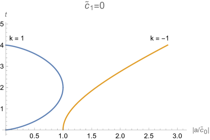
Figure 1: Plot of $t$ as a function of $|a/\tilde{c}_{0}|$ when $\tilde{c}_{1}=0$ for the cases $k=1$ and $k=-1$.

3.2 $w=0$ and $k=-1$

This case includes a nonrelativistic matter component for $k=-1$, in addition to the RT source. Perturbations around the previous solution with $\tilde{c}_{1}=0,\;k=-1$ are obtained for $c_{0}$ real and negative. Furthermore, eq. (3.26) allows for the initial conditions $\dot{a}=0$ and $\ddot{a}>0$ at $t=0$ provided that $-\tilde{c}_{0}-\tilde{c}_{1}=a(0)\geq 0$. The minimum value of the scale parameter, $a(0)$, can therefore be nonzero when $-\tilde{c}_{0}>\tilde{c}_{1}$, again describing a bouncing cosmology. An example, $\tilde{c}_{0}=-\frac{2}{3},\tilde{c}_{1}=\frac{1}{3}$, is plotted in figure 2, and it has $\ddot{a}>0$. The ratio $p_{{}_{\rm RT}}/\rho_{{}_{\rm RT}}$, evaluated on-shell, is not a constant for this case.

The previous solution, $\tilde{c}_{0}=-1\,,\tilde{c}_{1}=0$, as well as $\tilde{c}_{0}=0,\tilde{c}_{1}=1$ (corresponding to the absence of the RT source term), are shown in figure 2 for comparison purposes. The $\tilde{c}_{0}=0,\tilde{c}_{1}=1$ solution has $\dot{a}>1$, and so, from eq. (3.26), in order to perturb around that solution one would need that $\tilde{c}_{0}$ is purely imaginary. We find that these perturbations do not alter the $\tilde{c}_{0}=0,\tilde{c}_{1}=1$ solution significantly, and moreover do not appear to exhibit a positive acceleration.

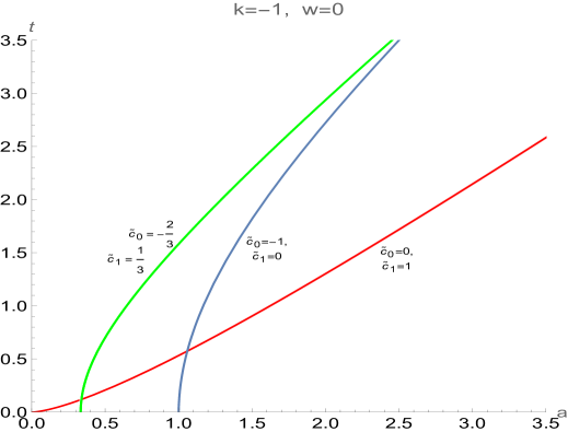
Figure 2: Plot of $t$ as a function of $a$ for $k=-1$, $w=0$ for the cases:
$\;i)\;\tilde{c}_{0}=-1,\tilde{c}_{1}=0\;$, $\;ii)\;\tilde{c}_{0}=-\frac{2}{3},\tilde{c}_{1}=\frac{1}{3}\;$ and $\;iii)\;\tilde{c}_{0}=0,\tilde{c}_{1}=1$.

3.3 $w=\frac{1}{3}$ and $k=-1$

This case includes a radiation component for $k=-1$, along with the Regge-Teitelboim source. Once again, perturbations around the solution with $\tilde{c}_{1}=0,\;k=-1$ are obtained for $c_{0}$ real and negative. Two kinds of initial conditions can be chosen: 1) $\dot{a}=0$ and $\ddot{a}>0$ at $t=0$ or 2) $a(0)=0$. From eq. (3.26), 1) is possible when $\frac{1}{2}(-\tilde{c}_{0}\pm\sqrt{\tilde{c}_{0}^{2}-4\tilde{c}_{1}})=a(0)\geq 0$. $a(0)$ then corresponds to a minimum, leading to a bouncing cosmology. 2) describes a singularity. Two nontrivial solutions are plotted in figure 3 $\;i)\;\tilde{c}_{0}=-.85,\tilde{c}_{1}=.15\;$, and $\;ii)\;\tilde{c}_{0}=-.8,\tilde{c}_{1}=.2\;$ $a$ has a nonzero minimum value for the former, while $a(0)=0$ for the latter. $\ddot{a}$ is positive for all $t$ for $\;i)$. On the other hand, for case $\;ii)$, starting from a value of $\dot{a}\approx 1$ in the limit $t\rightarrow 0$, the system initially decelerates, and then makes a transition to an accelerating phase ($\ddot{a}>0$) at a finite time $t$. More generally, from (3.26), such a transition occurs when $\dot{a}^{2}+\frac{\tilde{c}_{1}}{a^{2}}=1$.

Plots for $\;iii)\;\tilde{c}_{0}=-1,\tilde{c}_{1}=0\;$, and $\;iv)\;\tilde{c}_{0}=0,\tilde{c}_{1}=1$ are included in figure 3 for comparison purposes. As in the previous subsection, the $\tilde{c}_{0}=0,\tilde{c}_{1}=1$ solution has $\dot{a}>1$, and so, from eq. (3.26), perturbations around that solution are not possible for real values of $\tilde{c}_{0}$.

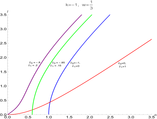
Figure 3: Plot of $t$ as a function of $a$ for $k=-1$, $w=\frac{1}{3}$ for the cases:
$\;i)\;\tilde{c}_{0}=-.85,\tilde{c}_{1}=.15\;$, $\;ii)\;\tilde{c}_{0}=-.8,\tilde{c}_{1}=.2\;,$ $\;iii)\;\tilde{c}_{0}=-1,\tilde{c}_{1}=0\;$, and $\;iv)\;\tilde{c}_{0}=0,\tilde{c}_{1}=1$.

4 Concluding remarks

The introduction of the RT source term in the Einstein equations leads to the modification of the Friedmann equations (3.26). The modification can be interpreted as a ‘dark force’, as it does not originate from the energy-momentum tensor. For the choice of embedding used in this paper, this force was given by (3.21). The modification of the Friedmann equations also gives an additional contribution to the density parameter (3.23). Exact solutions were found for the case where the usual energy-momentum tensor vanishes, which describe an accelerating universe when $k=-1$. This result persisted when a nonrelativistic matter component or radiation component was included. Moreover, for the case of a radiation component, there are $k=-1$ solutions which undergo a transition from a decelerating universe to an accelerating one.

Our results rely on a particular choice for the embedding[18]. It remains to be seen how robust the results are with respect to other choices of embeddings. Different ‘dark’ source terms $T_{{}_{\rm RT}}^{\mu\nu}$ will result from different choices of the embedding. These source terms are highly constrained by the current conservation conditions in (2.10), and by symmetry. For the case of the Robertson-Walker metric, with sources having the form in (3.4), the constraints are given by (3.13). For some embeddings, the conditions are too strong to allow for any modification of the Einstein equations. This is the case for the embedding of the $k=0$ Robertson-Walker metric in [18]. As $k=0$ is of physical relevance, it is worthwhile to do an extensive search for embeddings that produce analogous ‘dark’ contributions to the Friedmann equations. Another possible extension of this work is to relax the requirement that the background space is geometrically flat, and perhaps only demanding that it be Ricci flat.[17],[19] Of course, it is of interest to work towards constructing a more realistic cosmological model, one for example, that includes different matter-energy components, and combines the radiation and nonrelativistic matter eras. We plan to address these and other issues in the future.

Acknowledgment

A.S. is grateful for discussions with A. Pinzul.

References

- [1] T. Regge and C. Teitelboim, “General Relativity \‘a la string: a progress report,” in Proceedings of the First Marcel Grossmann Meeting (Trieste, Italy,1975), 77-87, ed. by R. Ruffini, North-Holland, Amsterdam, 1977; [arXiv:1612.05256 [hep-th]].
- [2] S. Deser, F. A. E. Pirani and D. C. Robinson, “Imbedding the G-String,” Phys. Rev. D 14, 3301-3303 (1976).
- [3] M. Pavsic, “On the Quantization of Gravity by Embedding Space-time in a Higher Dimensional Space,” Class. Quant. Grav. 2, 869 (1985).
- [4] V. Tapia, “GRAVITATION A LA STRING,” Class. Quant. Grav. 6, L49 (1989).
- [5] M. D. Maia, “On the Integrability Conditions for Extended Objects,” Class. Quant. Grav. 6, 173-183 (1989).
- [6] I. A. Bandos, “String - like description of gravity and possible applications for F theory,” Mod. Phys. Lett. A 12, 799-810 (1997).
- [7] R. Capovilla, A. Escalante, J. Guven and E. Rojas, “Hamiltonian dynamics of extended objects: Regge-Teitelboim model,” [arXiv:gr-qc/0603126 [gr-qc]].
- [8] H. Steinacker, “Emergent Geometry and Gravity from Matrix Models: an Introduction,” Class. Quant. Grav. 27, 133001 (2010).
- [9] D. N. Blaschke and H. Steinacker, “Curvature and Gravity Actions for Matrix Models,” Class. Quant. Grav. 27, 165010 (2010).
- [10] D. Z. Freedman, G. W. Gibbons and M. Schnabl, “Matrix cosmology,” AIP Conf. Proc. 743, no.1, 286-297 (2004) doi:10.1063/1.1848334 [arXiv:hep-th/0411119 [hep-th]].
- [11] D. Klammer and H. Steinacker, “Cosmological solutions of emergent noncommutative gravity,” Phys. Rev. Lett. 102, 221301 (2009).
- [12] S. W. Kim, J. Nishimura and A. Tsuchiya, “Expanding (3+1)-dimensional universe from a Lorentzian matrix model for superstring theory in (9+1)-dimensions,” Phys. Rev. Lett. 108, 011601 (2012);S. W. Kim, J. Nishimura and A. Tsuchiya, “Expanding universe as a classical solution in the Lorentzian matrix model for nonperturbative superstring theory,” Phys. Rev. D 86, 027901 (2012).
- [13] A. Stern, “Matrix Model Cosmology in Two Space-time Dimensions,” Phys. Rev. D 90, no.12, 124056 (2014); A. Chaney, L. Lu and A. Stern, “Matrix Model Approach to Cosmology,” Phys. Rev. D 93, no.6, 064074 (2016); A. Stern and C. Xu, “Signature change in matrix model solutions,” Phys. Rev. D 98, no.8, 086015 (2018).
- [14] A. Davidson, “Lambda = 0 cosmology of a brane - like universe,” Class. Quant. Grav. 16, 653-659 (1999).
- [15] R. Cordero, M. Cruz, A. Molgado and E. Rojas, “Quantum modified Regge-Teitelboim cosmology,” Gen. Rel. Grav. 46, 1761 (2014) [erratum: Gen. Rel. Grav. 46, 1770 (2014)].
- [16] S. A. Paston and A. A. Sheykin, “Embeddings for solutions of Einstein equations,” Theor. Math. Phys. 175, 806-815 (2013).
- [17] P. S. Wesson, “A Physical Interpretation of Kaluza-Klein Cosmology,” Astrophys. J. 394, 19-24 (1992).
- [18] J. Rosen, “Embedding of Various Relativistic Riemannian Spaces in Pseudo-Euclidean Spaces,” Rev. Mod. Phys. 37, 204 (1965).
- [19] C. Romero, R. K. Tavakol and R. Zalaletdinov, “The embedding of general relativity in five-dimensions,” Gen. Rel. Grav. 28, 365-376 (1996).