Information Decomposition Diagrams Applied beyond Shannon Entropy: a Generalization of Hu’s Theorem

Abstract

In information theory, one major goal is to find useful functions that summarize the amount of information contained in the interaction of several random variables. Specifically, one can ask how the classical Shannon entropy, mutual information, and higher interaction information functions relate to each other. This is formally answered by Hu’s theorem, which is widely known in the form of information diagrams: it relates disjoint unions of shapes in a Venn diagram to summation rules of information functions; this establishes a bridge from set theory to information theory. While a proof of this theorem is known, it has not yet been analyzed in detail in what generality it can be established. In this work, we view random variables together with the joint operation as a monoid that acts by conditioning on information functions, and entropy as the unique function satisfying the chain rule of information. This allows us to abstract away from Shannon’s theory and to prove a generalization of Hu’s theorem, which applies to Shannon entropy of countably infinite discrete random variables, Kolmogorov complexity, Tsallis entropy, (Tsallis) Kullback-Leibler Divergence, cross-entropy, submodular information functions, and the generalization error in machine learning. Our result implies for Chaitin’s prefix-free Kolmogorov complexity that the higher-order interaction complexities of all degrees are in expectation close to Shannon interaction information. For well-behaved probability distributions on increasing sequence lengths, this shows that asymptotically, the per-bit expected interaction complexity and information coincide, thus showing a strong bridge between algorithmic and classical information theory.

Index Terms: Information decomposition, information diagrams, chain rule, commutative idempotent monoids, Kolmogorov complexity, Shannon entropy, Tsallis entropy, Kullback-Leibler divergence, cross-entropy, generalization error

1 Introduction

Information diagrams, most often drawn for two or three random variables (see Figures 2 and 3), provide a concise way to visualize information functions. Not only do they show (conditional) Shannon entropy (Shannon, 1948), mutual information, and interaction information — also called co-information (Bell, 2003) — of several random variables in one overview — they also provide an intuitive account of the relations between these functions. Namely, we can read off summation rules of information functions from disjoint unions of the corresponding shapes.

This simple and well-known fact goes beyond just three variables: diagrams with four (see Figure 4) and more variables exist as well. Hu’s theorem (Hu, 1962; Yeung, 1991; 2002) renders all this mathematically precise by connecting the set-theoretic operations of union, intersection, and set difference to joint information, interaction information, and conditioning of information functions, respectively. The summation rules mentioned before are then summarized by just one property: the map, from sets to information functions, is a measure and thus turns disjoint unions into sums.

While Hu (1962) and later Yeung (1991) gave a proof of this theorem for Shannon entropy, they did not analyze in which generality it can be established. It seems a priori likely that a generalization beyond Shannon entropy is possible since the result is in its structure entirely combinatorial. Our aim is thus to find general algebraic structures giving rise to a generalized Hu theorem with a broad area of application.

Our claim is that the language employed in the foundations of information cohomology,  Baudot and Bennequin (2015), gives the perfect starting point for such an investigation. Namely, by replacing discrete random variables with partitions on a sample space, they give random variables the structure of a monoid that is commutative and idempotent. Furthermore, conditional information functions are formally described by a monoid action. And finally, the most basic information function that generates all others, Shannon entropy, is fully characterized as the unique function that satisfies the chain rule of information. We substantially generalize Hu’s theorem by giving a proof only based on the properties just mentioned, leading to new applications to Kolmogorov complexity, Kullback-Leibler divergence, and beyond.

To clarify, the main contribution of this work is not to provide major previously unknown ideas — indeed, our proof is very similar to the original one given in Yeung (1991) — but instead, to place and prove this result in its proper abstract context. This then reveals information diagrams for new information measures.

An Outline of this Work

We now outline our work for a general audience. In summary, Sections 2 and 3 provide a tutorial-style outline of classical Shannon information theory, formulated in a way that reveals the abstractions that we use. Section 4 — which can be read independently of the preceding sections — contains our main result, the generalized Hu theorem. Sections 5 and 6 apply the result to reveal information diagrams for Kolmogorov complexity and several other information functions. We conclude with a discussion in Section 7, followed by proofs in the appendices. Throughout, the text is written in a self-contained and explanatory way that should be readable to all mathematically interested readers without substantial background in (algorithmic) information theory. Below, we outline the different sections in more detail.

In Section 2, we give a self-contained treatment of Shannon entropy, mutual information, interaction information, and Hu’s theorem. We emphasize the algebraic relations of these functions over specifics of their definitions — most importantly, that the Shannon entropy $H(X,Y)$ of a joint random variable $(X,Y)$ is equal to the entropy of $X$, plus the entropy of $Y$ conditioned on $X$:

$$H(X,Y)=H(X)+H(Y\mid X).$$ (1)

This equation lies at the heart of connections to set theory and information diagrams due to its similarity with a basic equation of sets: the union of two sets, $\widetilde{X}\cup\widetilde{Y}$, can be written as a disjoint union as follows:

$$\widetilde{X}\cup\widetilde{Y}=\widetilde{X}\ \dot{\cup}\ \big{(}\widetilde{Y}\setminus\widetilde{X}\big{)}.$$

Hu’s theorem exploits this by constructing a measure that turns any union into a joint information term; any set difference into conditional information; any intersection into mutual information or — if more than two sets are involved — interaction information; and any disjoint union into a sum. The latter means that the theorem results in many more summation rules than just Equation (1), which is the main use of this result. To not restrict ourselves needlessly, we are slightly more general than prior work by allowing countably infinite sample spaces and random variables, thus making applications to Kolmogorov complexity in Section 5 viable.

The above suggests that algebraic relations of Shannon entropy alone make Hu’s theorem true. Thus, before giving the actual proof, we take a step back in Section 3 to reexamine the abstract properties of random variables and the corresponding information terms. The most important observation is that the information in a random variable is not changed if we replace it with an equivalent one. Here, a random variable $Y$ is said to be equivalent to $X$ if both are a deterministic function of each other. This notion is, for example, known in the context of separoids (Dawid, 2001), the mathematical framework for conditional independence; the relation to our work is explained by the equivalence of conditional independence to the vanishing of conditional mutual information.

Working with equivalence classes of random variables reveals further connections to set theory — for all random variables $X$ and $Y$, and sets $\widetilde{X}$ and $\widetilde{Y}$, the following properties hold:

commutativity: $$(X,Y)\text{ is equivalent to }(Y,X) \longleftrightarrow \widetilde{X}\cup\widetilde{Y}=\widetilde{Y}\cup\widetilde{X};$$

idempotence: $$(X,X)\text{ is equivalent to }X \longleftrightarrow \widetilde{X}\cup\widetilde{X}=\widetilde{X}.$$

We can then view Shannon entropy as a function on equivalence classes of random variables and formulate more succinctly some very basic algebraic properties:

• equivalence classes of random variables and the joint operation together form a commutative, idempotent monoid, or equivalently a join-semilattice;

• the space of information functions forms an abelian group; and

• conditional entropy can be reinterpreted by an additive monoid action; thereby, the monoid of equivalence classes acts on the abelian group of information functions.

This framework is inspired by the information cohomology theory in Baudot and Bennequin (2015). Their setup mainly differs by working with partition lattices on sample spaces instead of equivalence classes of random variables.

In Section 4, we then completely abstract away from the details of Shannon’s information theory and formulate our main result, the generalized Hu theorem, Theorem 4.2. Thereby, we take the properties described above as abstract assumptions. The theorem thus applies to any commutative, idempotent monoid acting on an abelian group, together with a corresponding function that simply needs to satisfy the chain rule, Equation (1). We also deduce a formulation for two-argument functions, Corollary 4.4, that makes the result applicable to Kolmogorov complexity later on. The proof we give is mostly combinatorial and based on an inclusion-exclusion type formula for the basic atoms of the sets. It carries strong similarities to the one given in Yeung (1991) for Shannon entropy itself.

To show the usefulness of this perspective, we naturally want to demonstrate the applicability beyond Shannon entropy. We do this in Sections 5 and 6. In Section 5, we analyze several versions of Kolmogorov complexity (Li and Vitányi, 1997). Different from Shannon entropy, this measures the information of individual binary strings instead of whole distributions over objects. The amount of information in a binary string $x$, $K(x)$, is quantified as the length of the shortest computer program that prints $x$ and then halts. One can also define the conditional information $K(x\mid y)$ as the length of the shortest program that, when given $y$ as an additional input, prints $x$ and then halts. An adapted version, Chaitin’s prefix-free Kolmogorov complexity $Kc$ (Chaitin, 1987), satisfies a chain rule up to a constant error (indicated by a plus):

$$Kc(x,y)\overset{+}{=}Kc(x)+Kc(y\mid x).$$

Binary strings do not form a commutative, idempotent monoid. But “inside $Kc$”, these crucial properties hold:

• commutativity: $Kc(x,y)\overset{+}{=}Kc(y,x)$, since one can write a computer program independent of $x$ and $y$ that translates $(x,y)$ to $(y,x)$, and vice versa;

• idempotence: $Kc(x,x)\overset{+}{=}Kc(x)$, since one can write a computer program independent of $x$ that translates $(x,x)$ to $x$, and vice versa.

As a result, we are able to recover the exact framework of our general theorem. We deduce Hu’s theorem for Chaitin’s prefix-free Kolmogorov complexity, Theorem 5.8.

We then combine Hu’s theorems for Shannon entropy and Kolmogorov complexity to generalize the well-known result that “expected Kolmogorov complexity is close to entropy” (Grünwald and Vitányi, 2008): general interaction complexity is close to interaction information. For the case of well-behaved sequences of probability measures on binary strings with increasing length, this leads to an asymptotic result: in the limit of infinite sequence length, the per-bit interaction complexity and interaction information coincide.

In Section 6, we then broaden our scope and look at further example applications. We systematically demonstrate the presence of all the abstract assumptions of our generalized theorem. This unlocks Hu’s theorem for Tsallis $\alpha$-entropy (Tsallis, 1988), Kullback-Leibler divergence, $\alpha$–Kullback-Leibler divergence, cross-entropy (Vigneaux, 2019), arbitrary functions on commutative, idempotent monoids, submodular information functions (Steudel et al., 2010), and the generalization error from machine learning (Shalev-Shwartz and Ben-David, 2014; Mohri et al., 2018). We also interpret the interaction terms of degree $2$ for both Kullback-Leibler divergence and the generalization error (Examples 6.4, 6.13). A more thorough interpretation of the resulting information diagrams is mostly left to future work.

Finally, in Section 7, we end with a discussion on the findings, the context, and future directions.

We collect most proofs in the Appendices A, B, C, D, E, and F. For some proofs, if they are especially valuable while being sufficiently easy to follow, we decided to keep them in the main text.

Preliminaries and Notation

We mainly assume the reader to be familiar with the basics of measure theory and probability theory. They can be learned from any book on the topic, for example Schilling (2017) or Tao (2013). The main concepts we assume to be known are $\sigma$-algebras, the Borel $\sigma$-algebra on $\mathds{R}^{n}$ (which is the $\sigma$-algebra generated by the open sets, or equivalently, all cuboids), measurable spaces, measures, measure spaces, probability measures, probability spaces, and random variables.

We do not assume any familiarity with information theory and will carefully introduce all basic notions. The same holds for the preliminaries of Kolmogorov complexity. The general nature of our work also demands us to use some basic concepts from abstract algebra. These are mainly abelian groups, (commutative, idempotent) monoids, and additive monoid actions. We will introduce them in the text and do not assume them to be known. However, we do presume that some basic familiarity with these concepts will be helpful.

On notation: to aid familiarity, we will start writing the Shannon entropy with the symbol $H$, but then switch to the notation $I_{1}$ once we embed Shannon entropy in the concept of interaction information, Definition 2.12. Similarly, we hoped to provide familiarity by writing conditional entropy as $H(Y\mid X)$ in the introduction; starting with Definition 2.7, we will replace this with $X.H(Y)=X.I_{1}(Y)$. This is the general notation of monoid actions and is thus preferable in our abstract context. Furthermore, for two disjoint sets $A$ and $B$, we write their union as $A\dot{\cup}B$. The number of elements in $A$ is written as $|A|$. The power set of $A$, i.e., the set of its subsets, is denoted $2^{A}$. And finally, the natural and binary logarithms of $x$ are denoted $\ln(x)$ and $\log(x)$, respectively.

2 Hu’s Theorem for Shannon Entropy of Countable Discrete Random Variables

In this tutorial-style section, we explain the original Hu theorem (Hu, 1962; Yeung, 1991) in the most familiar setting: discrete random variables, entropy, mutual information, and interaction information. For this, we only assume the reader to be familiar with well-known notions from probability theory such as measurable spaces, Borel measurable sets, sample spaces, probability measures, and random variables. Any book on measure theory can be used to learn these concepts, for example Tao (2013); Schilling (2017).

When we say a set is countable, then we mean it is finite or countably infinite. Whenever we talk about discrete measurable spaces, we mean countable measurable spaces in which all subsets are measurable. Thus, while our setting is familiar, we are more general than past research on Hu’s theorem in that we also allow for countably infinite discrete spaces; while this generalization is important for our applications to Kolmogorov complexity in Section 5.5, the reader may wish to ignore the additional complications by assuming that all spaces are finite.

We give ad hoc definitions of all the relevant information functions in Section 2.1. For the convenience of the reader, we also prove some basic and well-known properties of (joint) probability distributions. In Section 2.2, we provide intuitions for the meaning of Hu’s theorem for the simple case of two random variables. In Section 2.3 we then formulate Hu’s theorem for the general case of $n$ random variables. In Section 2.4, we explain the general use of this theorem and give some intuitions as to why it is true. These intuitions are intimately connected to the functional equation of entropy, the recursive definition of interaction information, and properties of averaged conditioning that resemble those of a monoid action. This motivates the more general and abstract treatment of the subject in subsequent sections.

Some technical considerations related to the measurability of certain functions in the infinite, discrete case are found in Appendix A. Most further proofs are collected in Appendix B.

2.1 Entropy, Mutual Information, and Interaction Information

We fix in this section a discrete sample space $\Omega$. Contrary to usual assumptions, we do not fix a probability measure on $\Omega$. We define

$$\Delta(\Omega)\coloneqq\bigg{\{}P:\Omega\to[0,1]\ \ \Big{|}\ \ \sum_{\omega\in\Omega}P(\omega)=1\bigg{\}}$$

as the space of probability measures on $\Omega$. Denote by $[0,1]^{\Omega}$ the set of functions from $\Omega$ to $[0,1]$, which we write as $(p_{\omega})_{\omega\in\Omega}$. Then we can also write

$$\Delta(\Omega)=\bigg{\{}{(p_{\omega})_{\omega\in\Omega}\in[0,1]^{\Omega}\ \ \Big{|}\ \ \sum_{\omega\in\Omega}p_{\omega}=1\bigg{\}}}.$$ (2)

Now, if $\Omega$ is finite, via an identification $[0,1]^{\Omega}\cong[0,1]^{|\Omega|}$ we can consider $[0,1]^{\Omega}$ together with the $\sigma$-algebra of Borel measurable sets. Then $\Delta(\Omega)$ inherits the structure of a measurable space, and we can thus talk about measurable functions on $\Delta(\Omega)$ — all classical information functions we consider in this work are of this type. Also in the case that $\Omega$ is infinite and discrete, $\Delta(\Omega)$ has the structure of a measurable space: we simply equip it with the smallest $\sigma$-algebra that makes all evaluation maps

$$\operatorname{ev}_{A}:\Delta(\Omega)\to\mathds{R},\ \ \ P\mapsto\operatorname{ev}_{A}(P)\coloneqq P(A)$$

for all subsets $A\subseteq\Omega$ measurable. In the finite case, this definition is equivalent with the one given before, as we show in Proposition A.1.

We remark that we do not distinguish between probability measures and their mass functions in the notation or terminology: for a subset $A\subseteq\Omega$ and a probability measure $P:\Omega\to[0,1]$, we simply set $P(A)\coloneqq\sum_{\omega\in A}P(\omega)$.

Our aim is the study of discrete random variables $X:\Omega\to E_{X}$. Here, being discrete means that $E_{X}$ — next to $\Omega$ — is discrete. Since $\Omega$ is discrete, $X$ can be any function and is then automatically measurable.

For any probability measure $P$ on $\Omega$ and any random variable $X:\Omega\to E_{X}$, we define the distributional law $P_{X}:E_{X}\to[0,1]$ as the unique probability measure with

$$P_{X}(x)\coloneqq P\big{(}X^{-1}(x)\big{)}=\sum_{\omega\in X^{-1}(x)}P(\omega)$$

for all $x\in X$. Clearly, $\sum_{x\in E_{X}}P_{X}(x)=1$, and thus $P_{X}\in\Delta(E_{X})$ is a well-defined probability measure. In the literature, $P_{X}$ is also called the push-forward or marginalization of $P$ along $X$ — we think of $X:\Omega\to E_{X}$ to “push” the probability measure $P\in\Delta(\Omega)$ to a probability measure $P_{X}\in\Delta(E_{X})$.

For the following definition of Shannon entropy, introduced in Shannon (1948); Shannon and Weaver (1964), we employ the convention $0\cdot\infty=0\cdot(-\infty)=0$ and $\ln(0)=-\infty$. Furthermore, set $\overline{\mathds{R}}\coloneqq\mathds{R}\cup\{+\infty\}$.

Definition 2.1 (Shannon Entropy).

Let $P\in\Delta(\Omega)$ be a probability measure. Then the Shannon entropy of $P$ is given by

$$H(P)\coloneqq-\sum_{\omega\in\Omega}P(\omega)\ln P(\omega)\in\overline{\mathds{R}}.$$

Here, $\ln:[0,\infty)\to\mathds{R}\cup\{-\infty\}$ is the natural logarithm. Now, let $X:\Omega\to E_{X}$ be a discrete random variable. The Shannon entropy of $X$ with respect to $P\in\Delta(\Omega)$ is given by

$$H(X;P)\coloneqq H(P_{X})=-\sum_{x\in E_{X}}P_{X}(x)\ln P_{X}(x)\in\overline{\mathds{R}}.$$

Note that $\operatorname{id}_{\Omega}:\Omega\to\Omega$, $\omega\mapsto\omega$ is a discrete random variable and that for all $P\in\Delta(\Omega)$, we have $P_{\operatorname{id}_{\Omega}}=P$ and therefore $H(\operatorname{id}_{\Omega};P)=H(P)$.

There are indeed examples of probability measures with infinite Shannon entropy. One characterization, taken from Baccetti and Visser (2013), is as follows.

Proposition 2.2 (See Proof B).

Let $\Omega=\mathds{N}_{\geq 1}$ be the natural numbers greater than $0$. Let $P\in\Delta(\Omega)$ be a probability measure. Assume that $P$ is ordered non-increasingly, i.e., $P(n+1)\leq P(n)$ for all $n\geq 1$. Then we have the equivalence

$$H(P)=\infty\quad\Longleftrightarrow\quad\sum_{n\geq 1}P(n)\ln n=\infty.$$

Example 2.3.

The following example is also taken from Baccetti and Visser (2013): Let $u\in(0,1]$ be any number, $\Omega=\mathds{N}_{\geq 2}$ the natural numbers larger than $1$ and $P:\Omega\to\mathds{R}$ given by

$$P(n)\coloneqq\frac{A}{n\cdot(\ln n)^{1+u}}\ \ ,$$

with $A$ chosen such that $\sum_{n\geq 2}P(n)=1$. Then $H(P)=\infty$, as can be seen with the help of Proposition 2.2, the well-known Cauchy condensation test for the convergence of series, and the divergence of the harmonic series. For the case $u=1$, this probability measure is related to integer coding (Grünwald, 2007), and we will encounter the related code later in Section 5.1, Equation (32).

Now, set

$$\Delta_{f}(\Omega)\coloneqq\Delta(\Omega)\setminus\{P\in\Delta(\Omega)\mid H(P)=\infty\}.$$

$\Delta_{f}(\Omega)$ is the measurable space of probability measures with finite entropy.

Lemma 2.4 (See Proof B).

Let $X:\Omega\to E_{X}$ be a discrete random variable and $P\in\Delta(\Omega)$ a probability measure. Then $H(X;P)\leq H(P)$. In particular, if $P\in\Delta_{f}(\Omega)$, then also $H(X;P)<\infty$.

This lemma makes the following definition well-defined:

Definition 2.5 (Entropy Function of a Random Variable).

Let $X:\Omega\to E_{X}$ be a discrete random variable. Then its entropy function or Shannon entropy is the measurable function

$$H(X):\Delta_{f}(\Omega)\to\mathds{R},\ \ \ P\mapsto H(X;P)$$

defined on probability measures with finite entropy. Its measurability is proven in Corollary A.6.

The reason we restrict to probability measures with finite entropy is that we can then easily build the difference of information functions, which is important in defining the higher order information functions later on.

We emphasize that, in our treatment, (discrete) random variables come not equipped with a probability measure, and thus the Shannon entropy $H(X)$ is not just a number, but a function with a probability measure as its input.

Our next goal is to inductively define the interaction information functions $I_{q}$ based on the definition of the Shannon entropy. We first need the notions of conditional probability measures and information functions: let $P:\Omega\to\mathds{R}$ be a probability measure and $X:\Omega\to E_{X}$ a discrete random variable. Then we define the conditional probability measure $P|_{X=x}:\Omega\to\mathds{R}$ by

$$P|_{X=x}(\omega)\coloneqq\begin{cases}\frac{P\big{(}\{\omega\}\cap X^{-1}(x)\big{)}}{P_{X}(x)},\ \ \ &P_{X}(x)\neq 0;\\ P(\omega),&P_{X}(x)=0.\end{cases}$$ (3)

Again, it can easily be verified that this is a probability measure, i.e., $\sum_{\omega\in\Omega}P|_{X=x}(\omega)=1$. For all $A\subseteq\Omega$, we then have

$$P|_{X=x}(A)=\begin{cases}\frac{P\big{(}A\cap X^{-1}(x)\big{)}}{P(X^{-1}(x))},\ \ \ &P_{X}(x)\neq 0;\\ P(A),&P_{X}(x)=0.\end{cases}$$

which we visualize in Figure 1. The following Lemma provides an important compatibility that is used in the definition below.

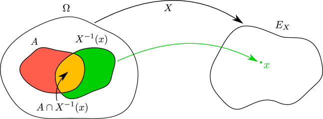
Figure 1: Let $X:\Omega\to E_{X}$ be a discrete random variable. We assume an underlying probability measure $P$ on $\Omega$. Let $x\in E_{X}$ with $P_{X}(x)=P(X^{-1}(x))\neq 0$. To compute the conditional probability $P|_{X=x}(A)$, one needs to divide the probability of the intersection $A\cap X^{-1}(x)$ by the probability of $X^{-1}(x)$.

Lemma 2.6 (See Proof B).

Let $X:\Omega\to E_{X}$ be a discrete random variable and $P\in\Delta_{f}(\Omega)$. Then for all $x\in E_{X}$, we also have $P|_{X=x}\in\Delta_{f}(\Omega)$.

For the following definition, recall that a series of real numbers converges absolutely if the series of its absolute values converges. It converges unconditionally if every reordering of the original series still converges with the same limit. According to the Riemann series theorem (MacRobert and Bromwich, 1926), both of these properties are equivalent.

Definition 2.7 (Conditionable Functions, Averaged Conditioning).

Let $F:\Delta_{f}(\Omega)\to\mathds{R}$ be a measurable function. $F$ is called conditionable if for all discrete random variables $X:\Omega\to E_{X}$ and all $P\in\Delta_{f}(\Omega)$, the sum

$$(X.F)(P)\coloneqq\sum_{x\in E_{X}}P_{X}(x)F(P|_{X=x})$$ (4)

converges unconditionally. Note that $P|_{X=x}\in\Delta_{f}(\Omega)$ by Lemma 2.6, which makes $F(P|_{X=x})$ in Equation (4) well-defined.

For all conditionable measurable functions $F:\Delta_{f}(\Omega)\to\mathds{R}$ and all discrete random variables $X:\Omega\to E_{X}$, the function $X.F:\Delta_{f}(\Omega)\to\mathds{R}$ is a measurable function by Corollary A.8, which we call the averaged conditioning of $F$ by $X$. The space of all conditionable measurable functions $F:\Delta_{f}(\Omega)\to\mathds{R}$ is denoted by $\operatorname{Meas}_{\operatorname{con}}(\Delta_{f}(\Omega),\mathds{R})$.

We now want to argue that this conditioning construction can be applied to the Shannon entropy of a random variable. The proof of this will use the chain rule of entropy, which requires us to consider the joint entropy of two random variables. If $X:\Omega\to E_{X}$ and $Y:\Omega\to E_{Y}$ are two (not necessarily discrete) random variables, then their (Cartesian) product $XY:\Omega\to E_{X}\times E_{Y}$ is defined by

$$(XY)(\omega)\coloneqq\big{(}X(\omega),Y(\omega)\big{)}\in E_{X}\times E_{Y}.$$ (5)

Since Cartesian products of discrete measurable spaces are again discrete, the product $XY$ is again discrete if $X$ and $Y$ are discrete. If we have two discrete random variables $X$ and $Y$ and a probability measure $P\in\Delta(\Omega)$, then this allows to consider $(P|_{X=x})_{Y}(y)$ for $(x,y)\in E_{X}\times E_{Y}$. In order to not overload notation, we will write this often as $P(y\mid x)$. Similarly, we will often write $P(x)\coloneqq P_{X}(x)$ and $P(\omega\mid x)\coloneqq P|_{X=x}(\omega)$.

Lemma 2.8 (See Proof B).

Let $X,Y$ be two discrete random variables on $\Omega$ and $P\in\Delta(\Omega)$ a probability measure. Then we get:

1. For all $(x,y)\in E_{X}\times E_{Y}$, we have

   $$P(x)\cdot P(y\mid x)=P(x,y).$$

2. For all $(x,y)\in E_{X}\times E_{Y}$ with $P(x,y)\neq 0$, we have

   $$(P|_{X=x})|_{Y=y}=P|_{XY=(x,y)}.$$

3. For all $x\in E_{X}$ we have

   $$P(x)=\sum_{y\in E_{Y}}P(x,y).$$

4. For all $y\in E_{Y}$ we have

   $$P(y)=\sum_{x\in E_{X}}P(x,y).$$

Lemma 2.9.

Let $Y$ be a discrete random variables on $\Omega$. Then $H(Y)$ is conditionable. More precisely, for another discrete random variable $X$ on $\Omega$ and $P\in\Delta_{f}(\Omega)$, $H(X;P)$ and $H(XY;P)$ are finite by Lemma 2.4, and we have

$$\big{[}X.H(Y)\big{]}(P)=H(XY;P)-H(X;P),$$

which results in $\big{[}X.H(Y)\big{]}(P)$ converging unconditionally.

Proof.

We have:

$$\big{[}X.H(Y)\big{]}(P) =\sum_{x\in E_{X}}P(x)H(Y;P|_{X=x})$$

$$=-\sum_{x\in E_{X}}P(x)\sum_{y\in E_{Y}}P(y\mid x)\ln P(y\mid x)$$

$$=-\sum_{(x,y)\in E_{X}\times E_{Y}}P(x,y)\ln\frac{P(x,y)}{P(x)} \big{(}\text{Lemma~{}\ref{lem:conditioning_simple_properties}, part 1}\big{)}$$

$$=-\sum_{(x,y)\in E_{X}\times E_{Y}}P(x,y)\ln P(x,y)-\Bigg{(}-\sum_{x\in E_{X}}P(x)\ln P(x)\Bigg{)} \big{(}\text{Lemma~{}\ref{lem:conditioning_simple_properties}, part 3}\big{)}$$

$$=H(XY;P)-H(X;P).$$

That concludes the proof. ∎

If we introduce some more notation, we can write the chain rule more succinctly: for two measurable information functions $F,G:\Delta_{f}(\Omega)\to\mathds{R}$, their sum $F+G$ is defined by $(F+G)(P)\coloneqq F(P)+G(P)$, which is again a measurable function. Similarly, $F-G$ can be defined. The trivial information function $0:\Delta_{f}(\Omega)\to\mathds{R}$ is the measurable function given by $0(P)\coloneqq 0$ for all $P\in\Delta_{f}(\Omega)$.

Proposition 2.10.

The following chain rule

$$H(XY)=H(X)+X.H(Y)$$

holds for arbitrary discrete random variables $X:\Omega\to E_{X}$ and $Y:\Omega\to E_{Y}$.

Proof.

The well-definedness of the measurable function $X.H(Y):\Delta_{f}(\Omega)\to\mathds{R}$ and the equation follow both from Lemma 2.9. ∎

We will also write $Y.F(P)\coloneqq(Y.F)(P)$. For example, if $F=H(X)$ is the Shannon entropy of the discrete random variable $X$, we write

$$Y.H(X;P)=Y.H(X)(P)=[Y.H(X)](P)=\sum_{y\in E_{Y}}P_{Y}(y)H(X;P|_{Y=y}).$$

We emphasize explicitly that $Y$ can not act on $H(X;P)$ since this is only a number, and not a measurable function. Nevertheless, we find the notation $Y.H(X;P)$ for $[Y.H(X)](P)$ convenient.

In the literature, one more often finds the notation $H(X|Y)$ for the conditional entropy. We choose the notation $Y.H(X)$ since it will make the connection to monoid actions clearer — they are generally notated in that way, see Definition 3.14. The following proposition states the most basic structural properties of the averaged conditioning that resemble those of an additive monoid action; this viewpoint will be central in our formulation and proof of Hu’s theorem in Section 4.

Proposition 2.11.

Let $X,Y$ be two discrete random variables on $\Omega$, $\bm{1}:\Omega\to\mathop{\scalebox{1.5}{\raisebox{-0.86108pt}{$\ast$}}}\coloneqq\{\ast\}$ a trivial random variable, and $F,G:\Delta_{f}(\Omega)\to\mathds{R}$ two conditionable measurable functions. Then the following hold:

1. $\bm{1}.F=F$;

2. $Y.F$ is also conditionable, and we have $X.(Y.F)=(XY).F$;

3. $F+G$ is also conditionable, and we have $X.(F+G)=X.F+X.G$.

Proof.

Properties 1 and 3 are clear. For $2$, let $P\in\Delta_{f}(\Omega)$ be arbitrary. We obtain

$$\big{[}X.(Y.F)\big{]}(P) =\sum_{x\in E_{X}}P(x)\cdot(Y.F)(P|_{X=x})$$

$$=\sum_{x\in E_{X}}P(x)\sum_{y\in E_{Y}}P(y\mid x)\cdot F\big{(}(P|_{X=x})|_{Y=y}\big{)}$$

$$=\sum_{(x,y)\in E_{X}\times E_{Y}}P(x,y)F\big{(}P|_{XY=(x,y)}\big{)} (\text{Lemma~{}\ref{lem:conditioning_simple_properties}, parts 1 and 2})$$

$$=\big{[}(XY).F\big{]}(P).$$

As the latter expression converges unconditionally due to $F$ being conditionable, also $\big{[}X.(Y.F)\big{]}(P)$ converges unconditionally. As $X$ and $P$ are arbitrary, $Y.F$ is conditionable. That finishes the proof. ∎

Next, we define mutual information and, more generally, interaction information — also called co-information (Bell, 2003). As we want to view interaction information as a “higher degree generalization” of entropy and treat both on an equal footing in Hu’s theorem, we now change the notation: for any discrete random variables $X$, we set $I_{1}(X)\coloneqq H(X)$.

Definition 2.12 (Mutual Information, Interaction Information).

Let $Y_{1},Y_{2}$ be two discrete random variables on $\Omega$. Then we define their mutual information, or interaction information of degree $2$, as the function $I_{2}(Y_{1};Y_{2}):\Delta_{f}(\Omega)\to\mathds{R}$ given by

$$I_{2}(Y_{1};Y_{2})\coloneqq I_{1}(Y_{1})-Y_{2}.I_{1}(Y_{1}).$$ (6)

Assume that $I_{q-1}$ is already defined. Assume also that $Y_{1},\dots,Y_{q}$ are $q$ discrete random variables on $\Omega$. Then we define $I_{q}(Y_{1};\dots;Y_{q}):\Delta_{f}(\Omega)\to\mathds{R}$, the interaction information of degree $q$, as the function

$$I_{q}(Y_{1};\dots;Y_{q})\coloneqq I_{q-1}(Y_{1};\dots;Y_{q-1})-Y_{q}.I_{q-1}(Y_{1};\dots;Y_{q-1}).$$

In this vein, we call entropy $I_{1}$ interaction information of degree $1$.

Remark 2.13.

Note that what we call interaction information is in the literature sometimes called (higher/multivariate) mutual information. In that case, the term $J_{q}(Y_{1};\dots;Y_{q})\coloneqq(-1)^{q+1}I_{q}(Y_{1};\dots;Y_{q})$ is called interaction information, see for example Baudot (2021).

Proposition 2.14.

For all $q\geq 1$ and all discrete random variables $Y_{1},\dots,Y_{q}$, $I_{q}(Y_{1};\dots;Y_{q}):\Delta_{f}(\Omega)\to\mathds{R}$ is a well-defined conditionable measurable function.

Proof.

$I_{1}(Y_{1})$ is conditionable by Lemma 2.9. Assuming by induction that $I_{q-1}(Y_{1};\dots;Y_{q-1})$ is well-defined and conditionable, we obtain the following: $Y_{q}.I_{q-1}(Y_{1};\dots;Y_{q-1})$ is well-defined and conditionable by Proposition 2.11, part 2, and $I_{q}(Y_{1};\dots;Y_{q})$ is well-defined and conditionable by Proposition 2.11, part 3. ∎

2.2 Hu’s Theorem for Two Random Variables

For two sets $A$ and $B$, we will by $A\dot{\cup}B$ denote the disjoint union of $A$ and $B$, in the case that $A$ and $B$ are in fact disjoint.

We now look closer at the sequence of functions $I_{1},I_{2},I_{3},\dots$ and want to provide an intuition for a connection to measures and Hu’s theorem. For simplicity, here we only consider the case of two discrete random variables $X:\Omega\to E_{X}$ and $Y:\Omega\to E_{Y}$. We step-by-step go through a number of equations appearing for information functions, and build analogs to equations in basic set theory. These analogs are eventually made concrete by Hu’s theorem. We give a visual summary of this section in Figure 2.

We now write the Shannon entropy as $I_{1}$, so the chain rule from Proposition 2.10 becomes

$$I_{1}(XY)=I_{1}(X)+X.I_{1}(Y),$$ (7)

and the definition of $I_{2}$ given Equation (6) becomes

$$I_{2}(X;Y)=I_{1}(X)-Y.I_{1}(X).$$ (8)

Note that we can also change the roles of $X$ and $Y$ in these two equations.

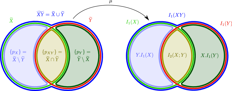
Figure 2: Hu’s theorem, visualized for two discrete random variables $X$ and $Y$, and for entropy $I_{1}$ and mutual information $I_{2}$. On the left-hand-side, we can see Equations (9), (11), and  (13) visualized. The measure $\mu$ then turns sets into information functions and disjoint unions into sums. On the right-hand-side we see a visualization of the resulting Equations (7), (10), and (2.2).

Equation (7) reminds of the set-theoretic rule

$$\widetilde{X}\cup\widetilde{Y}=\widetilde{X}\ \dot{\cup}\ \big{(}\widetilde{Y}\setminus\widetilde{X}\big{)},$$ (9)

which holds for every two sets $\widetilde{X},\widetilde{Y}$. We can rearrange Equation (8) to

$$I_{1}(X)=Y.I_{1}(X)+I_{2}(X;Y),$$ (10)

which reminds of the rule

$$\widetilde{X}=\big{(}\widetilde{X}\setminus\widetilde{Y}\big{)}\ \dot{\cup}\ \big{(}\widetilde{X}\cap\widetilde{Y}\big{)}.$$ (11)

We can find a decomposition similar to Equation (10) for $I_{1}(Y)$ as follows:

$$I_{1}(Y) =I_{1}(YX)-Y.I_{1}(X) (\text{Eq.~{}\eqref{eq:cocycle_condition_simplified}})$$

$$=I_{1}(XY)-Y.I_{1}(X) (\text{Obvious symmetry})$$

$$=\big{[}X.I_{1}(Y)+I_{1}(X)\big{]}-Y.I_{1}(X) (\text{Eq.~{}\eqref{eq:cocycle_condition_simplified}})$$

$$=X.I_{1}(Y)+\big{[}I_{1}(X)-Y.I_{1}(X)\big{]} (\text{Rebracketing})$$

$$=X.I_{1}(Y)+I_{2}(X;Y), (\text{Eq.~{}\eqref{eq:def_I_2_simplified}})$$ (12)

which reminds of the rule

$$\widetilde{Y}=\big{(}\widetilde{Y}\setminus\widetilde{X}\big{)}\ \dot{\cup}\ \big{(}\widetilde{X}\cap\widetilde{Y}\big{)}.$$ (13)

All these comparisons together suggest the following correspondence between operations on discrete random variables and information functions on the one hand, and set-theoretic relations on the other hand:

1. The entropy $I_{1}(XY)$ of a joint variable $XY$ corresponds to the union of sets $\widetilde{X}\cup\widetilde{Y}$;

2. The mutual information $I_{2}(X;Y)$ of two discrete random variables corresponds to the intersection of sets $\widetilde{X}\cap\widetilde{Y}$;

3. Conditioning $X.I_{1}(Y)$ corresponds to a set difference, or relative complement, $\widetilde{Y}\setminus\widetilde{X}$;

4. Any disjoint union decomposition of a set leads to a summation rule of the corresponding information function.

The last property is crucial for turning all these analogies into something concrete: measures turn disjoint unions of sets into sums of real numbers, and thus one can wonder whether information functions can be expressed using measures. Our situation mainly differs in that in our case, we consider sums of information functions and not sums of real numbers. This, however, only requires a slight adaptation of the concept of a measure, as we demonstrate next.

We now construct an explicit (generalized) measure for our simplified setting. Thus, we want (finite) sets $\widetilde{X}$ and $\widetilde{Y}$ with union $\widetilde{XY}=\widetilde{X}\cup\widetilde{Y}$ and a function $\mu:2^{\widetilde{XY}}\to\operatorname{Meas}_{\operatorname{con}}(\Delta_{f}(\Omega),\mathds{R})$ mapping subsets in $\widetilde{XY}$ (i.e., elements of the power set $2^{\widetilde{XY}}$) to conditionable measurable functions from $\Delta_{f}(\Omega)$ to $\mathds{R}$, such that the following properties hold:

1. $\mu(A_{1}\dot{\cup}A_{2})=\mu(A_{1})+\mu(A_{2})$ for all disjoint $A_{1},A_{2}\subseteq\widetilde{XY}$;

2. $I_{1}(X)=\mu\big{(}\widetilde{X}\big{)}$;

3. $I_{1}(Y)=\mu\big{(}\widetilde{Y}\big{)}$;

4. $Y.I_{1}(X)=\mu\big{(}\widetilde{X}\setminus\widetilde{Y}\big{)}$;

5. $X.I_{1}(Y)=\mu\big{(}\widetilde{Y}\setminus\widetilde{X}\big{)}$;

6. $I_{2}(X;Y)=\mu\big{(}\widetilde{X}\cap\widetilde{Y}\big{)}$; and

7. $I_{1}(XY)=\mu\big{(}\widetilde{XY}\big{)}$.

We choose the simplest sets $\widetilde{X}$, $\widetilde{Y}$ in “general position” to each other, meaning that neither of the sets is completely contained in the other, and their intersection is nonempty. Then, we define $\mu$ on it as required by the equations derived so far. Let $p_{X}$, $p_{Y}$, and $p_{XY}$ three arbitrary (abstract) atoms — a terminology we borrow from Yeung (1991) — and define

$$\widetilde{X} \coloneqq\big{\{}p_{X},p_{XY}\big{\}},$$

$$\widetilde{Y} \coloneqq\big{\{}p_{XY},p_{Y}\big{\}},$$

$$\widetilde{XY} \coloneqq\widetilde{X}\cup\widetilde{Y}=\big{\{}p_{X},p_{XY},p_{Y}\big{\}}.$$

Then, define $\mu:2^{\widetilde{XY}}\to\operatorname{Meas}_{\operatorname{con}}(\Delta_{f}(\Omega),\mathds{R})$ by

$$\mu(p_{X}) \coloneqq Y.I_{1}(X),$$

$$\mu(p_{XY}) \coloneqq I_{2}(X;Y),$$

$$\mu(p_{Y}) \coloneqq X.I_{1}(Y),$$

$$\forall A\subseteq\widetilde{XY}:\mu(A) \coloneqq\sum_{p\in A}\mu(p).$$

Then, by what we have shown before, all of the rules 1–7 from above are satisfied; we achieved our goal. All of this is visualized in Figure 2.

2.3 A Formulation of Hu’s Theorem for $n$ Random Variables

Armed with the intuitions from the last section, we now formulate Hu’s theorem for interaction information $I_{q}$, $q\geq 1$. The result was originally proven in Hu (1962) and reinvestigated in Yeung (1991; 2002). Our formulation is closest to the one presented in Baudot et al. (2019) and mainly differs from earlier work by also considering countably infinite discrete random variables.

Let $n\geq 0$ be a natural number and $[n]\coloneqq\{1,\dots,n\}$. We assume we have $n$ discrete random variables $X_{1},\dots,X_{n}$ on $\Omega$. For any $I\subseteq[n]$, we write

$$X_{I}\coloneqq\prod_{i\in I}X_{i}:\Omega\to\prod_{i\in I}E_{X_{i}},\quad\omega\mapsto\big{(}X_{i}(\omega)\big{)}_{i\in I}$$

for the joint of all the $X_{i}$ with $i\in I$. Define $M\coloneqq\{X_{I}\mid I\subseteq[n]\}$ as the set of these joint variables.

Denote by $\operatorname{Meas}_{\operatorname{con}}(\Delta_{f}(\Omega),\mathds{R})$ the space of conditionable measurable functions $F:\Delta_{f}(\Omega)\to\mathds{R}$. For every $q\geq 1$ we can now view the interaction information of degree $q$ as a function

$$I_{q}:M^{q} \to\operatorname{Meas}_{\operatorname{con}}(\Delta_{f}(\Omega),\mathds{R})$$

$$(X_{L_{1}},\dots,X_{L_{q}}) \mapsto I_{q}(X_{L_{1}};\dots;X_{L_{q}}).$$

Hu’s theorem will show that there exists a certain measure with values in $\operatorname{Meas}_{\operatorname{con}}(\Delta_{f}(\Omega),\mathds{R})$ that turns a certain set into the information function $X_{J}.I_{q}(X_{L_{1}};\dots;X_{L_{q}})$.

For having a measure, we also need a set on which this measure will “live”. As in the case of two variables in the last section, we want to have a set $\widetilde{X}_{i}$ for each variable $X_{i}$, and furthermore, we want these sets to be in “general position”: we require that for each $\emptyset\neq I\subseteq[n]$, the set $\bigcap_{i\in I}\widetilde{X}_{i}\setminus\bigcup_{j\in[n]\setminus I}\widetilde{X}_{j}$ is nonempty. Furthermore, we want the simplest collection of sets with these properties. We construct this as follows: for each $\emptyset\neq I\subseteq[n]$, we denote by $p_{I}$ an abstract atom. The only property we require of them is to be pairwise different, i.e., $p_{I}\neq p_{J}$ if $I\neq J$. Then, set $\widetilde{X}$ as the set of all these atoms:

$$\widetilde{X}\coloneqq\big{\{}p_{I}\mid\emptyset\neq I\subseteq[n]\big{\}}.$$ (14)

The atoms $p_{I}$ represent all smallest parts (the intersections of sets with indices in $I$ minus the sets with indices in $[n]\setminus I$) of a general Venn diagram for $n$ sets.

For $i\in[n]$, we denote by $\widetilde{X}_{i}\coloneqq\left\{p_{I}\in\widetilde{X}|i\in I\right\}$ a set which we can imagine to be depicted by a ”circle” corresponding to the variable $X_{i}$ and with $\widetilde{X}_{I}\coloneqq\bigcup_{i\in I}\widetilde{X}_{i}$ the union of the “circles” corresponding to the joint variable $X_{I}$. Clearly, we have $\widetilde{X}=\widetilde{X}_{[n]}$. This is actually the simplest construction that leads to the $\widetilde{X}_{i}$ being in general position, as the following Lemma shows:

Lemma 2.15.

It holds

$$\bigcap_{i\in I}\widetilde{X}_{i}\ \ \setminus\ \ \bigcup_{j\in[n]\setminus I}\widetilde{X}_{j}=\{p_{I}\}$$

for all $\emptyset\neq I\subseteq[n]$.

Proof.

We have

$$\bigcap_{i\in I}\widetilde{X}_{i}\ \ \setminus\ \ \bigcup_{j\in[n]\setminus I}\widetilde{X}_{j} =\Big{\{}p_{J}\ \ \big{|}\ \ \forall i\in I:i\in J\ \ \wedge\ \ \forall j\in[n]\setminus I:j\notin J\Big{\}}$$

$$=\Big{\{}p_{J}\ \ \big{|}\ \ I\subseteq J\ \ \wedge\ \ \big{(}[n]\setminus I\big{)}\cap J=\emptyset\Big{\}}$$

$$=\{p_{I}\}.$$

∎

We remark that $\widetilde{X}$ depends on $n$ and could therefore also be written as $\widetilde{X}(n)$. We will in most cases abstain from this to not overload the notation. In general, $\widetilde{X}$ has $2^{n}-1$ elements. Therefore, for $n=2$, $n=3$ and $n=4$, $\widetilde{X}$ has $3$, $7$, and $15$ elements, respectively, see Figures 2, 3 and 4.

Similar to the concept of an $I$-measure in Yeung (1991), we now define information measures:

Definition 2.16 (Information Measure).

Let $\widetilde{X}=\widetilde{X}(n)$ and $\operatorname{Meas}_{\operatorname{con}}(\Delta_{f}(\Omega),\mathds{R})$ be defined as above. Let $2^{\widetilde{X}}$ be the power set of $\widetilde{X}$, i.e., the set of its subsets. An information measure is a function

$$\mu:2^{\widetilde{X}}\to\operatorname{Meas}_{\operatorname{con}}(\Delta_{f}(\Omega),\mathds{R})$$

with the property

$$\mu(A_{1}\cup A_{2})=\mu(A_{1})+\mu(A_{2})$$

for every two disjoint subsets $A_{1},A_{2}\subseteq\widetilde{X}$.

Note: our concept of an information measure is not a generalization of the concept of submodular information measures defined in Steudel et al. (2010). We consider their work shortly in Section 6.6.

A consequence of Definition 2.16 is

$$\mu\left(\bigcup_{k=1}^{m}A_{k}\right)=\sum_{k=1}^{m}\mu(A_{k})$$

whenever $A_{k}\subseteq\widetilde{X}$ are pairwise disjoint. Also, $\mu(\emptyset)=\mu(\emptyset)+\mu(\emptyset)$ implies $\mu(\emptyset)=0$.

We remark that there is nothing special about the set $\widetilde{X}$ and that one could also define information measures on other sets. However, since we only use it in the context of our set $\widetilde{X}$, we stick with this terminology.

We now state Hu’s theorem (Hu, 1962), which mainly differs by us making a construction of the information measure explicit, and by allowing for countably infinite discrete random variables:

Theorem 2.17 (Hu’s theorem).

Let $n\geq 0$ and $X_{1},\dots,X_{n}$ be discrete random variables on $\Omega$. Let $\widetilde{X}=\widetilde{X}(n)$ be defined as above. Then there is an information measure $\mu:2^{\widetilde{X}}\to\operatorname{Meas}_{\operatorname{con}}\big{(}\Delta_{f}(\Omega),\mathds{R}\big{)}$ such that for all $q=1,2,\dots$ and for all $J,L_{1},\dots,L_{q}\subseteq[n]$, the following identity holds:

$$X_{J}.I_{q}(X_{L_{1}};\dots;X_{L_{q}})=\mu\Bigg{(}\bigcap_{k=1}^{q}\widetilde{X}_{L_{k}}\setminus\widetilde{X}_{J}\Bigg{)}.$$ (15)

Concretely, $\mu$ can be defined as the unique information measure that is on individual atoms $p_{I}\in\widetilde{X}$ defined by

$$\mu(p_{I})\coloneqq\sum_{\emptyset\neq K\supseteq I^{c}}(-1)^{|K|+|I|+1-n}\cdot I_{1}(X_{K}),$$ (16)

where $I^{c}=[n]\setminus I$ is the complement of $I$ in $[n]$.

Remark 2.18.

We make the following remarks:

1. In the finite discrete case, it is known that also the reverse of that theorem is true if one requires one additional mild assumption. Namely, we will show in the generalization Theorem 4.2 that, whenever one has a sequence of functions $F_{1},\dots,F_{q}$ that satisfy Equation (15) for an information measure $\mu$, then $F_{1}$ satisfies the chain rule of Proposition 2.10, and $F_{q}$ is inductively built from $F_{q-1}$ as $I_{q}$ is built from $I_{q-1}$. Additionally, assuming a so-called joint-locality property, Baudot and Bennequin (2015) were able to show that a function $F_{1}$ that satisfies the chain rule must already coincide with Shannon entropy: $F_{1}=I_{1}$. It is then immediately clear that $F_{q}=I_{q}$ for all $q\geq 1$.

2. It follows immediately from this theorem that for all $L_{1},\dots,L_{q},J\subseteq[n]$ and all $l\geq 0$, one has

   $$X_{J}.I_{q}(X_{L_{1}};\dots;X_{L_{q}}) =\mu\Bigg{(}\bigcap_{k=1}^{q}\widetilde{X}_{L_{k}}\setminus\widetilde{X}_{J}\Bigg{)}$$

   $$=\mu\Bigg{(}\bigcap_{k=1}^{q}\widetilde{X}_{L_{k}}\cap\bigcap_{k=1}^{l}\widetilde{X}\setminus\widetilde{X}_{J}\Bigg{)}$$

   $$=I_{q+l}(X_{L_{1}};\dots;X_{L_{q}};X_{[n]};\dots;X_{[n]}).$$

   This means that generally, $I_{q+l}$ is a generalization of $I_{q}$ for all $q\geq 1,l\geq 0$. Entropy is, for example, just mutual information with itself: $I_{1}(X)=I_{2}(X;X)$.

3. One usually finds a version of this theorem in which an arbitrary probability measure $P\in\Delta_{f}(\Omega)$ is fixed, so that both sides of Equation (15) are just numbers. We can easily recover this by defining $\mu^{P}(A)\coloneqq[\mu(A)](P)$ and $I_{q}^{P}(Y_{1};\dots;Y_{q})\coloneqq I_{q}(Y_{1};\dots;Y_{q};P)$. $\mu^{P}:2^{\widetilde{X}}\to\mathds{R}$ is then in the usual terminology called a signed measure.

   The word “signed” expresses that this measure can also take on negative values. Indeed, let $X,Y,Z$ be binary random variables with values in $\{0,1\}$, and write $p_{xyz}=P_{XYZ}(x,y,z)$. If

   $$p_{000}=1/4,\ \ \ p_{011}=1/4,\ \ \ p_{101}=1/4,\ \ \ \text{and }\ p_{110}=1/4$$

   then $I_{3}^{P}(X;Y;Z)=-1$. This is actually the minimum of $I_{3}$ for the case of three binary random variables, and the only other joint probability distribution achieving this minimum is given by

   $$p_{001}=1/4,\ \ \ p_{010}=1/4,\ \ \ p_{100}=1/4,\ \ \ \text{and }\ p_{111}=1/4.$$

   This, and a generalization to larger numbers of binary random variables, was proven in Baudot et al. (2019); Baudot (2021), highlighting also similarities to the topological notion of Borromean links.

2.4 A Motivation for Hu’s Theorem for $n$ Random Variables

Here, we want to build an intuition for what the theorem is useful for and why it is true.

The main use is the following: oftentimes, one needs to prove some identity of information functions of the form $F+G=H$. $F,G,H$ may all be of the form $X_{J}.I_{q}(X_{L_{1}};\dots;X_{L_{q}})$, and so by Hu’s theorem we find subsets $A^{F},A^{G},A^{H}\subseteq\widetilde{X}$ such that

$$F=\mu\big{(}A^{F}\big{)},\quad G=\mu\big{(}A^{G}\big{)},\quad H=\mu\big{(}A^{H}\big{)}.$$

If it can be proven that

$$A^{F}\dot{\cup}A^{G}=A^{H},$$

we easily obtain the desired result by using that $\mu$, as an information measure, turns disjoint unions into sums:

$$F+G=\mu\big{(}A^{F}\big{)}+\mu\big{(}A^{G}\big{)}=\mu\big{(}A^{F}\dot{\cup}A^{G}\big{)}=\mu\big{(}A^{H}\big{)}=H.$$

We present an example of this strategy in Figure 3. Note that in this and the following figures, we write sets $I=\{i_{1},\dots,i_{k}\}$ for simplicity just as the sequence $i_{1}i_{2}\dots i_{k}$.

Additional applications can be found in Yeung (1991), where many information inequalities are deduced using information diagrams. Furthermore, note that in applications, one often has specific knowledge about the underlying joint probability distribution that leads to certain parts of the information diagram having measure zero. This is, for example, the case for Markov chains, which were investigated in (Hu (1962), Theorem 3) and Kawabata and Yeung (1992); their information diagrams have a fan-like structure. In Yeung et al. (2019), this is generalized to characterize Markov random fields in information-theoretic terms. Further applications are discussed in Section 7.4.

These use cases also highlight that we do not care about what the elements in $\widetilde{X}$ are. They are just abstract atoms that are arranged in such a way that we can construct the information measure $\mu$; the existence of such an information measure is the correct abstraction for summarizing the truth of a large number of equations that follow the pattern we just described. The general picture for the case of four variables is drawn in Figure 4.

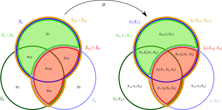
Figure 3: A visualization of Hu’s theorem for three discrete random variables $X_{1},X_{2}$ and $X_{3}$. On the left-hand-side, three subsets of the abstract set $\widetilde{X}$ are emphasized, namely $\widetilde{X}_{12}\cap\widetilde{X}_{13}$, $\widetilde{X}_{1}\setminus\widetilde{X}_{3}$, and $\widetilde{X}_{12}\cap\widetilde{X}_{3}$. On the right-hand-side, Equation (15) turns them into the information functions $I_{2}(X_{12};X_{13})$, $X_{3}.I_{1}(X_{1})$, and $I_{2}(X_{12};X_{3})$, respectively. Many decompositions of information functions into sums directly follow from the theorem by using that $\mu$ turns disjoint unions into sums, as exemplified by the equation $I_{2}(X_{12};X_{13})=X_{3}.I_{1}(X_{1})+I_{2}(X_{12};X_{3})$.

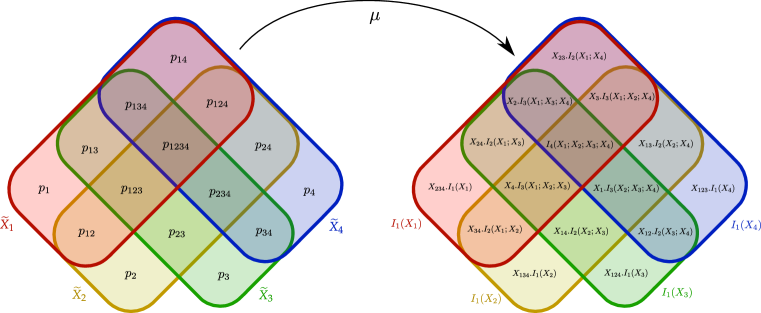
Figure 4: A visualization of Hu’s theorem for four discrete random variables $X_{1},X_{2},X_{3}$, and $X_{4}$. To reduce clutter, we restrict to a visualization of the abstract sets $\widetilde{X}_{i}$ and the atoms $p_{I}$, as well as the corresponding information functions. On the right-hand-side, for computing $\mu(p_{I})$ for the $15$ atoms $p_{I}$, we use that $\{p_{I}\}=\bigcap_{i\in I}\widetilde{X}_{i}\setminus\bigcup_{j\in[4]\setminus I}\widetilde{X}_{j}$ and Equation (15).

Why is Hu’s theorem true? While we do not give the full proof here, we outline the general structure. We will see in the generalization in Section 4 that an inductive argument is possible: first, we will show that the chain rule of entropy, Equation (7), and the rule $\bm{1}.F=F$ from Proposition 2.11 is enough to proof Hu’s theorem for the case $q=1$. That is, one can show that there is an information measure $\mu:2^{\widetilde{X}}\to\operatorname{Meas}_{\operatorname{con}}\big{(}\Delta_{f}(\Omega),\mathds{R}\big{)}$ such that for all $J,L_{1}\subseteq[n]$, we have

$$\mu\big{(}\widetilde{X}_{L_{1}}\setminus\widetilde{X}_{J}\big{)}=X_{J}.I_{1}(X_{L_{1}}).$$ (17)

The hard part in this step will be the construction of the information measure $\mu$, for which one needs to define $\mu(p_{I})$ for all $\emptyset\neq I\subseteq[n]$ by an inclusion-exclusion formula of entropy terms. After this is done, this can be inductively generalized to all $q>1$. We demonstrate this now for the case $q=2$: let $J,L_{1},L_{2}\subseteq[n]$ be arbitrary and assume Equation (17) holds. We obtain:

$$X_{J}.I_{2}\big{(}X_{L_{1}};X_{L_{2}}\big{)} =X_{J}.\big{(}I_{1}(X_{L_{1}})-X_{L_{2}}.I_{1}(X_{L_{1}})\big{)} (\text{Definition~{}\ref{def:interaction_information}})$$

$$=X_{J}.I_{1}(X_{L_{1}})-X_{J}.\big{(}X_{L_{2}}.I_{1}(X_{L_{1}})\big{)} (\text{Proposition~{}\ref{pro:conditioning_rules}, part 3})$$

$$=X_{J}.I_{1}(X_{L_{1}})-(X_{J}X_{L_{2}}).I_{1}(X_{L_{1}}) (\text{Proposition~{}\ref{pro:conditioning_rules}, part 2})$$

$$=X_{J}.I_{1}(X_{L_{1}})-X_{J\cup L_{2}}.I_{1}(X_{L_{1}}) (\star)$$

$$=\mu\big{(}\widetilde{X}_{L_{1}}\setminus\widetilde{X}_{J}\big{)}-\mu\big{(}\widetilde{X}_{L_{1}}\setminus\widetilde{X}_{J\cup L_{2}}\big{)} (\text{Equation~{}\eqref{eq:case_q_1}})$$

$$=\mu\big{(}\widetilde{X}_{L_{1}}\setminus\widetilde{X}_{J}\big{)}-\mu\big{(}\widetilde{X}_{L_{1}}\setminus(\widetilde{X}_{J}\cup\widetilde{X}_{L_{2}})\big{)} (\text{clear})$$

$$=\mu\big{(}\widetilde{X}_{L_{1}}\cap\widetilde{X}_{L_{2}}\setminus\widetilde{X}_{J}\big{)}, (\star\star)$$

which shows the desired result. In step $(\star)$, we replace the joint variable $X_{J}X_{L_{2}}$ with $X_{J\cup L_{2}}$. Note that these discrete random variables are not the same: they can differ in the order and multiplicity of their factors, especially if $J\cap L_{2}\neq\emptyset$. However, it will turn out that the variables $X_{J}X_{L_{2}}$ and $X_{J\cup L_{2}}$ are in a precise sense equivalent, which can be imagined as “they contain the same information”, and thus conditioning on them produces the same result. More abstractly, this equivalence will be the result of interpreting certain collections of random variables as an idempotent, commutative monoid. In step $(\star\star)$, we use

$$\big{(}\widetilde{X}_{L_{1}}\cap\widetilde{X}_{L_{2}}\setminus\widetilde{X}_{J}\big{)}\dot{\cup}\big{(}\widetilde{X}_{L_{1}}\setminus(\widetilde{X}_{J}\cup\widetilde{X}_{L_{2}})\big{)}=\widetilde{X}_{L_{1}}\setminus\widetilde{X}_{J}$$ (18)

and that $\mu$, being an information measure, turns disjoint unions into sums. We visualize this last step in Figure 5.

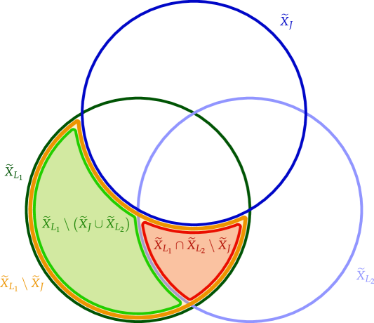
Figure 5: This figure shows graphically why the set-theoretic identity Equation (18) is true; it is crucial in the inductive step of our proof for Hu’s theorem.

This induction idea suggests the structure for the coming two sections: in Section 3 we will study a notion of equivalence of random variables and will show that the interaction information $I_{q}$ and the conditioning of information functions only depend on equivalence classes and not specific representatives. This allows to replace $X_{J}X_{L_{2}}$ by $X_{J\cup L_{2}}$ in the argument above. Additionally, equivalence classes of random variables can formally be seen as elements of a monoid, and so we can interpret Proposition 2.11 as the properties of a monoid action.

The above proof idea shows that to establish Hu’s theorem we need some abstract properties like the chain rule of entropy, the inductive construction of $I_{q}$ from $I_{q-1}$, and the properties of a monoid action. The explicit formula of entropy given in Definition 2.1 is not crucial, once these abstract properties are already established. This is why we can state Hu’s theorem in more general terms for arbitrary finitely generated, commutative, idempotent monoids acting on an abelian group in Section 4. We will then give a proof based on the outline from above.

3 Equivalence Classes and Monoids of Random Variables

In this section, we establish abstract properties of interaction information in relation to discrete random variables which will lead to a generalization of Hu’s theorem in Section 4. In Section 3.1, we study equivalence classes of random variables and show that interaction information $I_{q}$ and the averaged conditioning of discrete random variables on information functions is preserved under equivalence. In Section 3.2, we then study monoids of random variables and view averaged conditioning as a monoid action on $\operatorname{Meas}_{\operatorname{con}}\big{(}\Delta_{f}(\Omega),\mathds{R}\big{)}$. For the discrete case, equivalence classes of random variables are in a one-to-one correspondence with partitions on a sample space; these partitions were the starting point in Baudot and Bennequin (2015). Most proofs for this section can be found in Appendix C.

The content of this section is largely not new, and differs from previous work mainly by a strong emphasis of the abstract properties of information functions in relation to discrete random variables.

3.1 Equivalence Classes of Random Variables

We want to define a certain notion of equivalence of random variables in such a way that equivalent random variables have the same information content. To not restrict ourselves needlessly, we will for a moment work with general measurable spaces and not assume that they are discrete.

Let $\Omega$ be a nonempty measurable space that serves as our sample space. We study random variables $X:\Omega\to E_{X}$, where $E_{X}$ is some (not necessarily discrete) measurable space.

For two random variables $X$ and $Y$ on $\Omega$, we write $X\precsim Y$ if there is a measurable function $f_{XY}:E_{Y}\to E_{X}$ such that $f_{XY}\circ Y=X$:

This diagram is commutative, meaning that each route from $\Omega$ to $E_{X}$ results in the same random variable.

Intuitively, $X\precsim Y$ means that “$X$ is a function of $Y$”. It implies that if we know a sample of $Y$, we automatically know the corresponding sample of $X$, but not necessarily vice versa. Thus, $X$ can be seen as containing “a subset of the information of $Y$”, a viewpoint which we will make precise in Proposition 3.1. We also want to mention that the definition of $\precsim$ is equivalent to a preorder put forward in the context of conditional independence relations (Dawid, 1979; 1980; 2001). The latter work defines in their Section 6.2: $X\precsim Y$ if for all $\omega,\omega^{\prime}\in\Omega$, the following implication holds true:

$$Y\big{(}\omega\big{)}=Y\big{(}\omega^{\prime}\big{)}\ \ \Longrightarrow\ \ X\big{(}\omega\big{)}=X\big{(}\omega^{\prime}\big{)}.$$

It is straightforward to show that this coincides with our own definition.

Clearly, our relation is reflexive: $X=\text{id}_{E_{X}}\circ X$ implies $X\precsim X$. It is also transitive: if $X\precsim Y$ and $Y\precsim Z$, then there are measurable functions $f_{XY}$ and $f_{YZ}$ such that $X=f_{XY}\circ Y$ and $Y=f_{YZ}\circ Z$, respectively. It follows $X=(f_{XY}\circ f_{YZ})\circ Z$ and thus $f_{XZ}\coloneqq f_{XY}\circ f_{YZ}$ witnesses that $X\precsim Z$. Being reflexive and transitive, this relation is by definition a preorder.

we define $X\sim Y$ iff $X\precsim Y$ and $Y\precsim X$. In diagrams, this looks as follows, with both triangles commuting:

Note, however, that we do not necessarily have $f_{XY}\circ f_{YX}=\operatorname{id}_{E_{X}}$ or $f_{YX}\circ f_{XY}=\operatorname{id}_{E_{Y}}$, so this is not a notion of an isomorphism.

From the fact that $\precsim$ is reflexive and transitive, it follows immediately that $\sim$ is reflexive, transitive, and symmetric (meaning that $X\sim Y$ implies $Y\sim X$), i.e., it is indeed an equivalence relation. We denote by $\left[X\right]$ the equivalence class of the random variable $X$.

We now restrict to the case where the sample space $\Omega$ is non-empty and discrete and only consider discrete random variables $X:\Omega\to E_{X}$. In this setting, we can study how equivalence of random variables interacts with the interaction information functions $I_{q}$ and conditioning of functions. We first show that Shannon entropy is compatible with equivalence of random variables, and will then inductively generalize this to all $I_{q}$. The following proposition is a generalization of Lemma 2.4:

Proposition 3.1 (See Proof C).

Let $Y\precsim X$ be two discrete random variables on $\Omega$. Then we have $I_{1}(Y)\leq I_{1}(X)$ as functions on $\Delta_{f}(\Omega)$, meaning that $I_{1}(Y;P)\leq I_{1}(X;P)$ for all $P\in\Delta_{f}(\Omega)$. In particular, if $X$ and $Y$ are equivalent (i.e., $X\precsim Y$ and $Y\precsim X$), then $I_{1}(X)=I_{1}(Y)$.

Remark 3.2.

As is easy to show and well-known, using conditional entropy, one can even get an equivalence: one has $Y\precsim X$ if and only if $X.I_{1}(Y)=0$.

Proposition 3.3 (See Proof C).

Let $X\sim Y$ be two equivalent discrete random variables on $\Omega$. Then for all conditionable measurable functions $F:\Delta_{f}(\Omega)\to\mathds{R}$ we have $X.F=Y.F$.

We will prove the reverse of the preceding proposition in Proposition 3.10, after we understand the connection between equivalence classes of random variables and partitions on the sample space.

Proposition 3.4.

Let $q\geq 1$ and $Y_{1},\dots,Y_{q}$ and $Z_{1},\dots,Z_{q}$ be two collections of discrete random variables on $\Omega$ such that $Y_{k}\sim Z_{k}$ for all $k=1,\dots,q$. Then $I_{q}(Y_{1};\dots;Y_{q})=I_{q}(Z_{1};\dots;Z_{q})$.

Proof.

For $q=1$, this was shown in Proposition 3.1. We proceed by induction and assume it is already known for $q-1$. We obtain

$$I_{q}(Y_{1};\dots;Y_{q}) =I_{q-1}(Y_{1};\dots;Y_{q-1})-Y_{q}.I_{q-1}(Y_{1};\dots;Y_{q-1}) (\text{Definition~{}\ref{def:interaction_information}})$$

$$=I_{q-1}(Z_{1};\dots,Z_{q-1})-Y_{q}.I_{q-1}(Z_{1};\dots;Z_{q-1}) (\text{Induction hypothesis})$$

$$=I_{q-1}(Z_{1};\dots;Z_{q-1})-Z_{q}.I_{q-1}(Z_{1};\dots;Z_{q-1}) (\text{Propositions~{}\ref{pro:averaged_conditioning_equivalence},\ref{pro:interaction_information_pliable}})$$

$$=I_{q}(Z_{1};\dots;Z_{q}). (\text{Definition~{}\ref{def:interaction_information}})$$

That finishes the proof. ∎

This proposition shows that interaction information is naturally defined for collections of equivalence classes of random variables, instead of the random variables themselves. This viewpoint becomes fruitful for a generalization of Hu’s theorem.

3.2 Monoids of Random Variables

For the time being, we again consider a general measurable sample space $\Omega$ that is not necessarily discrete, and random variables $X:\Omega\to E_{X}$ with a general measurable value space $E_{X}$. For two random variables $X$ and $Y$, we define the joint variable $XY:\Omega\to E_{X}\times E_{Y}$ by $(XY)(\omega)\coloneqq(X(\omega),Y(\omega))$. We now show that the equivalence relation on random variables interacts nicely with the joint-operation; these rules will allow us to define monoids of (equivalence classes of) random variables.

Lemma 3.5.

Let $X,Y,Z,X^{\prime}$, and $Y^{\prime}$ be random variables on $\Omega$. Let $\bm{1}:\Omega\to\mathop{\scalebox{1.5}{\raisebox{-0.86108pt}{$\ast$}}}$ be a trivial random variable, with $\mathop{\scalebox{1.5}{\raisebox{-0.86108pt}{$\ast$}}}=\{\ast\}$ a measurable space with one element. Then the following properties hold:

1. If $X\sim X^{\prime}$ and $Y\sim Y^{\prime}$, then $XY\sim X^{\prime}Y^{\prime}$;

2. $\bm{1}X\sim X\sim X\bm{1}$;

3. $(XY)Z\sim X(YZ)$;

4. $XY\sim YX$;

5. $XX\sim X$.

Proof.

All of these statements are clear. For an illustration of the method, we prove the last statement: look at the diagram

where we set $\Delta(x)\coloneqq(x,x)$ and $\operatorname{pr}_{1}(x,y)\coloneqq x$. We have

$$(\Delta\circ X)(\omega)=\Delta(X(\omega))=(X(\omega),X(\omega))=(XX)(\omega),$$

which implies $\Delta\circ X=XX$ and thus $XX\precsim X$. We also have

$$(\operatorname{pr}_{1}\circ XX)(\omega)=\operatorname{pr}_{1}\big{(}(XX)(\omega)\big{)}=\operatorname{pr}_{1}(X(\omega),X(\omega))=X(\omega),$$

which implies $\operatorname{pr}_{1}\circ XX=X$ and thus $X\precsim XX$. Together, it follows $X\sim XX$. ∎

We make the following definition which resembles the rules $1$ to $4$ from above:

Definition 3.6 ((Commutative, Idempotent) Monoid).

Let $M$ be a set, $\bm{1}\in M$ a distinguished element (the unit or neutral element), and $\cdot:M\times M\to M$ a function. Then the triple $(M,\cdot,\bm{1})$ (often abbreviated just $M$) is called a monoid if the following conditions hold:

1. neutral element: $\bm{1}\cdot m=m=m\cdot\bm{1}$ for all $m\in M$;

2. associativity: $(m\cdot n)\cdot o=m\cdot(n\cdot o)$ for all $m,n,o\in M$.

If additionally the following condition holds, then $M$ is called a commutative monoid:

1. commutativity: $m\cdot n=n\cdot m$ for all $m,n\in M$.

If, on top of conditions $1$ and $2$, the following condition holds, then $M$ is called an idempotent monoid:

1. idempotence: $m\cdot m=m$ for all $m\in M$.

We remark that a commutative, idempotent monoid is algebraically the same as a join-semilattice (sometimes also called bounded join-semilattice), i.e., a partially ordered set which has a bottom element (corresponding to $\bm{1}\in M$) and binary joins (corresponding to the multiplication in a monoid). The partial order can be reconstructed from a commutative, idempotent monoid $M$ by writing $m\leq n$ if $m\cdot n=n$. The language of join-semilattices is, for example, used in the development of the theory of conditional independence (Dawid, 2001).

Example 3.7.

The classical example of a commutative monoid is $(\mathds{N},+,0)$, where $\mathds{N}$ is the natural numbers including zero.

For every set $\Sigma$, the power set $2^{\Sigma}$ gives rise to two commutative, idempotent monoids:

• $\big{(}2^{\Sigma},\cap,\Sigma\big{)}$ — in this monoid, $\Sigma$ is the unit of intersection since $\Sigma\cap A=A$ for all $A\in 2^{\Sigma}$; and

• $\big{(}2^{\Sigma},\cup,\emptyset\big{)}$ — in this monoid, $\emptyset$ is the unit of union since $\emptyset\cup A=A$ for all $A\in 2^{\Sigma}$.

These two monoids are dual to each other, since one can be transformed in the other by forming the complements of sets:

$$\big{(}A\cap B\big{)}^{c}=A^{c}\cup B^{c},\ \ \big{(}A\cup B\big{)}^{c}=A^{c}\cap B^{c},\ \ \Sigma^{c}=\emptyset.$$

Every abelian group $(G,+,0)$ is also a commutative monoid; we will define abelian groups in Definition 3.12.

We now come to the most important commutative, idempotent monoid of our work.

Proposition 3.8 (See Proof C).

Let $\widehat{M}=\{X:\Omega\to E_{X}\}_{X}$ be a collection of random variables with the following two properties:

1. There is a random variable $\bm{1}:\Omega\to\mathop{\scalebox{1.5}{\raisebox{-0.86108pt}{$\ast$}}}$ in $\widehat{M}$ which has a one-point set $\mathop{\scalebox{1.5}{\raisebox{-0.86108pt}{$\ast$}}}=\{\ast\}$ as the target;

2. For every two $X,Y\in\widehat{M}$ there exists a $Z\in\widehat{M}$ such that $XY\sim Z$.

Let $\left[X\right]$ denote the equivalence class of $X$ under the relation $\sim$. Define $M\coloneqq\widehat{M}/\sim$ as the collection of equivalence classes of elements in $\widehat{M}$. Define $\left[X\right]\cdot\left[Y\right]\coloneqq\left[Z\right]$ for any $Z\in\widehat{M}$ with $XY\sim Z$. If $M$ is a set, then the triple $(M,\cdot,\left[\bm{1}\right])$ is a commutative, idempotent monoid.

For the interested reader, for discrete $\Omega$, we next compare this with the monoid of partitions on $\Omega$, also called partition lattice (Grätzer, 2011), which is an alternative formalization used in Baudot and Bennequin (2015). Namely, define

$$M^{p}\coloneqq\Big{\{}X\subseteq 2^{\Omega}\ \ \big{|}\ \ X\text{ is a partition of }\Omega\Big{\}}.$$

Here, a partition is a set of nonempty, pairwise disjoint subsets whose union is $\Omega$. One can multiply partitions as follows:

$$X\cdot Y\coloneqq\Big{\{}A\cap B\ \ \big{|}\ \ A\in X,\ \ B\in Y,\ \ A\cap B\neq\emptyset\Big{\}},$$

which gives $M^{p}$ the structure of a commutative, idempotent monoid with neutral element $\{\Omega\}$.

Proposition 3.9 (See Proof C).

Consider the special case that $\Omega$ is discrete, and that $\widehat{M}$ is the collection of all discrete random variables on $\Omega$. Set $M^{r}\coloneqq M\coloneqq\widehat{M}/\sim$ as in Proposition 3.8. Then $M^{r}$ and $M^{p}$ are isomorphic monoids.

In the Proof C, the partition of a (equivalence class of a) random variable is constructed as the set of the preimages of all its values.

This shows that both formalizations are equally valid. We do not currently know whether the construction using partitions can usefully be generalized to non-discrete $\Omega$, and what the relation of such a construction to our definition of equivalence classes of random variables would be.

With this result we obtain the reverse of Proposition 3.3:

Proposition 3.10 (See Proof C).

Let $X:\Omega\to E_{X}$ and $Y:\Omega\to E_{Y}$ be two discrete random variables. Then the following two statements are equivalent:

• $X\sim Y$;

• For all conditionable measurable functions $F:\Delta_{f}(\Omega)\to\mathds{R}$, we have $X.F=Y.F$.

We can now study finite monoids of random variables as instances of the construction in Proposition 3.8. For that, we repeat some notation from Section 2.3: Let $n\geq 0$ be a natural number. Let $X_{1},\dots,X_{n}$ be fixed random variables on $\Omega$. Define $[n]\coloneqq\{1,\dots,n\}$. For arbitrary $I\subseteq[n]$, define $X_{I}\coloneqq\prod_{i\in I}X_{i}$, the joint of the variables $X_{i}$ for $i\in I$. For $X_{J}$ and $X_{I}$, note that we have the equivalence $X_{J}X_{I}\sim X_{J\cup I}$, which follows from the rule $XX\sim X$ by deleting copies of variables $X_{i}$ with $i\in J\cap I$, and by reordering the factors with the rule $XY\sim YX$. Note that $X_{\emptyset}:\Omega\to\mathop{\scalebox{1.5}{\raisebox{-0.86108pt}{$\ast$}}}=\{\ast\}$ is a trivial random variable.

Definition 3.11 (Monoid of $X_{1},\dots,X_{n}$).

The monoid $\operatorname{M}(X_{1},\dots,X_{n})$ of the variables $X_{1},\dots,X_{n}$ consists of the following data:

1. The elements are equivalence classes $\left[X_{I}\right]$ for $I\subseteq[n]$.

2. The multiplication is given by $\left[X_{J}\right]\cdot\left[X_{I}\right]=\left[X_{J\cup I}\right]$.

3. $\bm{1}\coloneqq\left[X_{\emptyset}\right]$ is the neutral element with respect to multiplication.

This is a well-defined commutative, idempotent monoid by Proposition 3.8.

We remark here that the structure of this monoid depends on the variables $X_{1},\dots,X_{n}$. For example, if $X_{1}=\dots=X_{n}=X$ are all identical random variables, then $\operatorname{M}(X_{1},\dots,X_{n})=\big{\{}\bm{1},[X]\big{\}}$ has maximally two elements. Additionally, $\bm{1}=[X]$ happens if and only if $X$ takes only one value.

Definition 3.12 (Abelian Group).

Let $G$ be a set, $0\in G$ a distinguished element, and $+:G\times G\to G$ a function. Then the triple $(G,+,0)$ (often abbreviated just $G$) is called an abelian group if the following properties are satisfied for all $g,h,k\in G$:

1. neutral element: $0+g=g=g+0$;

2. associativity: $(g+h)+k=g+(h+k)$;

3. inverse: there is an element $-g\in G$ such that $g+(-g)=(-g)+g=0$;

4. commutativity: $g+h=h+g$.

The first three properties make $G$ a group, and the last property makes it abelian, by definition. Properties 1 and 2 imply that the element $-g$ in property 3 is unique. Similarly, $0$ is the only element satisfying property 1.

Note that while we are mainly interested in idempotent monoids, any interesting abelian group is not idempotent: if it had this property, then from $x+x=x$ we could always deduce $x=0$, and thus the group would be trivial.

Example 3.13.

There are many examples of abelian groups, e.g., the integers $(\mathds{Z},+,0)$, the real numbers $(\mathds{R},+,0)$, or the group $(\operatorname{SO}(2),\circ,\operatorname{id}_{\mathds{R}^{2}})$ of rotations of the plane $\mathds{R}^{2}$.

The most important abelian group in our context is the group $\operatorname{Meas}_{\operatorname{con}}\big{(}\Delta_{f}(\Omega),\mathds{R}\big{)}=\Big{(}\operatorname{Meas}_{\operatorname{con}}\big{(}\Delta_{f}(\Omega),\mathds{R}\big{)},+,0\Big{)}$ of conditionable measurable functions from $\Delta_{f}(\Omega)$ to $\mathds{R}$, where $\Omega$ is a discrete sample space, and $\Delta_{f}(\Omega)$, as before, the set of probability measures on $\Omega$ with finite entropy. In the group, given two functions $F,G\in\operatorname{Meas}_{\operatorname{con}}(\Delta_{f}(\Omega),\mathds{R})$, we define $F+G$ as the function $(F+G)(P)\coloneqq F(P)+G(P)$; the function $0:\Delta_{f}(\Omega)\to\mathds{R}$ is given by $0(P)=0$ for all $P\in\Delta_{f}(\Omega)$; and finally, given a function $F\in\operatorname{Meas}_{\operatorname{con}}(\Delta_{f}(\Omega),\mathds{R})$, the function $-F$ is defined by $(-F)(P)\coloneqq-(F(P))$.

Definition 3.14 ((Additive) Monoid Action).

Let $M=(M,\cdot,\bm{1})$ be a monoid and $G=(G,+,0)$ an abelian group. Then an additive monoid action (or monoid action for short) of $M$ on $G$, by definition, is a function $.:M\times G\to G$ with the following properties for all $m,n\in M$ and $g,h\in G$:

1. trivial action: $\bm{1}.g=g$;

2. associativity: $m.(n.g)=(m\cdot n).g$;

3. additivity: $m.(g+h)=m.g+m.h$.

$G$, together with the action $.:M\times G\to G$, is sometimes also called an $M$-module.

Now we again restrict to the case that the sample space $\Omega$ and value spaces $E_{X}$ of random variables are discrete.

Proposition 3.15.

Let $M$ be a monoid of (equivalence classes of) discrete random variables on $\Omega$ as in Proposition 3.8. Let $G=\operatorname{Meas}_{\operatorname{con}}\big{(}\Delta_{f}(\Omega),\mathds{R}\big{)}$ be the group of conditionable measurable functions from $\Delta_{f}(\Omega)$ to $\mathds{R}$. Then the averaged conditioning $.:M\times G\to G$ given by

$$\big{(}\left[X\right].F\big{)}(P)\coloneqq\big{(}X.F\big{)}(P)=\sum_{x\in E_{X}}P_{X}(x)F(P|_{X=x})$$

is a well-defined monoid action.

Proof.

The action is well-defined by Proposition 3.3 and Proposition 2.11, part 2. It is a monoid action by Proposition 2.11. ∎

Summary 3.16.

We now summarize the abstract properties of interaction information $I_{q}$ that we have explained until now. Let $M$ be a commutative, idempotent monoid of discrete random variables as in Proposition 3.8. By abuse of notation, we do not distinguish between random variables and their equivalence classes, i.e., we write $Y$ instead of $\left[Y\right]$. Denote by $G\coloneqq\operatorname{Meas}_{\operatorname{con}}\big{(}\Delta_{f}(\Omega),\mathds{R}\big{)}$ the group of conditionable measurable functions from $\Delta_{f}(\Omega)$ to $\mathds{R}$. By Proposition 3.15, averaged conditioning $.:M\times G\to G$ is a well-defined monoid action.

By Proposition 3.4, we can view $I_{q}$ as a function $I_{q}:M^{q}\to G$ that is defined on tuples of equivalence classes of discrete random variables. By Proposition 2.10, entropy $I_{1}$ satisfies the equation

$$I_{1}(XY)=I_{1}(X)+X.I_{1}(Y)$$

for all $X,Y\in M$, where $X.I_{1}(Y)$ is the result of the action of $X\in M$ on $I_{1}(Y)\in G$ via averaged conditioning. Finally, by Definition 2.12, for all $q\geq 2$ and all $Y_{1},\dots,Y_{q}\in M$, one has

$$I_{q}(Y_{1};\dots;Y_{q})=I_{q-1}(Y_{1};\dots;Y_{q-1})-Y_{q}.I_{q-1}(Y_{1};\dots;Y_{q-1}).$$

When restricting to the case that $M=\operatorname{M}(X_{1},\dots,X_{n})$ is generated by finitely many discrete random variables $X_{i}$, then the properties summarized here are all one needs to prove Hu’s theorem, Theorem 2.17. This generalized view and the proof is the topic of the next section.

4 A Generalization of Hu’s Theorem

In this section, we formulate and prove a generalization of Hu’s theorem, Theorem 2.17. Our treatment can be read mostly independently from the preceding sections. First, in Section 4.1, we formulate the main result of this work, Theorem 4.2, together with its Corollary 4.4 that allows it to be applied to Kolmogorov complexity in Section 5 and the generalization error in Section 6. The formulation relies on a group-valued measure whose construction we motivate visually in Section 4.2. The proofs can then be found in Appendix D.

Afterwards, in Section 4.3, we deduce some general consequences about how (conditional) interaction terms of different degrees can be related to each other. Finally, in Section 4.4, we investigate some simple “relative computations” that allow one to sometimes ignore certain variables when proving equations.

4.1 A Formulation of the Generalized Hu Theorem

Let $M$ be an commutative, idempotent monoid, see Definition 3.6. We assume that $M$ is finitely generated, meaning there are elements $X_{1},\dots,X_{n}\in M$ such that all elements in $M$ can be written as arbitrary (possibly empty, to get the trivial element $1\in M$) finite products of the elements $X_{1},\dots,X_{n}$. Since $M$ is commutative, every product of elements $X_{i}$ can be reordered such that all $X_{i}$ with the same index $i$ are next to each other. Then, since $M$ is idempotent, we can reduce the product further until each $X_{i}$ appears maximally once. This means that general elements in $M$ are of the form $X_{I}=\prod_{i\in I}X_{i}$ for some subset $I\subseteq[n]=\{1,\dots,n\}$, and that $X_{I}X_{J}\coloneqq X_{I}\cdot X_{J}=X_{I\cup J}$. This fully mirrors the situation with the monoid of random variables $\operatorname{M}(X_{1},\dots,X_{n})$, which we considered in Definition 3.11.

Additionally, fix any abelian group $G$ and any additive monoid action $.:M\times G\to G$, see Definitions 3.12 and 3.14, respectively.

As in Section 2.3, let $\widetilde{X}=\widetilde{X}(n)=\big{\{}p_{I}\mid\emptyset\neq I\subseteq[n]\big{\}}$. Also, let $\widetilde{X}_{i}$ and $\widetilde{X}_{I}$ again be the sets of atoms $p_{J}$ with $i\in J$ and the union of all $\widetilde{X}_{i}$ with $i\in I$, respectively.

We can also define a slight generalization of our concept of an information measure from before. Remember that for a set $\Sigma$, $2^{\Sigma}$ is its powerset, i.e., the set of its subsets.

Definition 4.1 (($G$-Valued) Measure).

Let $G$ be an abelian group and $\Sigma$ a set. A $G$-valued measure is a function $\mu:2^{\Sigma}\to G$ with the property

$$\mu(A_{1}\cup A_{2})=\mu(A_{1})+\mu(A_{2})$$

for all disjoint $A_{1},A_{2}\subseteq\Sigma$. As for the case of information measures, we obtain $\mu(\emptyset)=0$, and $\mu$ turns arbitrary finite disjoint unions into the corresponding finite sums.

inline]I should drop the finite generatednedd of the monoid!! It’s somehow annoying in my new paper!!

inline]Maybe I should write the measure always as $\widetilde{F}$? It’s more suggestive and makes clear that it depends on the cochain.

Theorem 4.2 (Generalized Hu Theorem; See Section D.1 and Proof D.1).

Let $M$ be a commutative, idempotent monoid generated by $X_{1},\dots,X_{n}$, $G$ an abelian group, $.:M\times G\to G$ an additive monoid action, and $\widetilde{X}=\widetilde{X}(n)$ as defined in Section 2.4.

1. Assume $F_{1}:M\to G$ is a function that satisfies the following chain rule: for all $X,Y\in M$, one has

   $$F_{1}(XY)=F_{1}(X)+X.F_{1}(Y).$$ (19)

   Construct $F_{q}:M^{q}\to G$ for $q\geq 2$ inductively by

   $$F_{q}(Y_{1};\dots;Y_{q})\coloneqq F_{q-1}(Y_{1};\dots;Y_{q-1})-Y_{q}.F_{q-1}(Y_{1};\dots;Y_{q-1})$$ (20)

   for all $Y_{1},\dots,Y_{q}\in M$.

   Then there exists a $G$-valued measure $\mu:2^{\widetilde{X}}\to G$ such that for all $q\geq 1$ and $J,L_{1},\dots,L_{q}\subseteq[n]$, the following identity holds:

   $$X_{J}.F_{q}(X_{L_{1}};\dots;X_{L_{q}})=\mu\Bigg{(}\bigcap_{k=1}^{q}\widetilde{X}_{L_{k}}\setminus\widetilde{X}_{J}\Bigg{)}.$$ (21)

   Concretely, one can define $\mu$ as the unique $G$-valued measure that is on individual atoms $p_{I}\in\widetilde{X}$ defined by

   $$\mu(p_{I})\coloneqq\sum_{\emptyset\neq K\supseteq I^{c}}(-1)^{|K|+|I|+1-n}\cdot F_{1}(X_{K}),$$ (22)

   where $I^{c}=[n]\setminus I$ is the complement of $I$ in $[n]$.

2. Conversely, assume that $\mu:2^{\widetilde{X}}\to G$ is a $G$-valued measure. Assume there is a sequence of functions $F_{q}:M^{q}\to G$ which “satisfy Hu’s theorem” with respect to $\mu$, meaning that they satisfy Equation (21). Then $F_{1}$ satisfies Equation (19) and $F_{q}$ is related to $F_{q-1}$ as in Equation (20).

We will first explicitly construct the $G$-valued measure $\mu$ in Section 4.2. Then, we will prove the theorem together with the following Corollary 4.4 in Appendix D.1, with the last step in Proof D.1.

Remark 4.3.

We make three remarks here:

• Theorem 4.2, together with Summary 3.16, immediately provide a proof for Hu’s theorem for Shannon entropy, Theorem 2.17.

• Note that the generators $X_{1},\dots,X_{n}$ in Theorem 4.2 are not determined by $M$. Thus, one can choose $X_{1},\dots,X_{n}$ based on the application at hand, and obtain a corresponding Hu’s theorem. We make use of this in Section 4.4. Furthermore, $M$ does not need to be finitely generated, as long as the theorem is always applied to a submonoid generated by finitely many elements $X_{1},\dots,X_{n}$.

• In Remark 2.18, part 3, we mentioned that the signed measure corresponding to more than two random variables and a fixed probability measure can also take negative values. In the general case, the situation is even more peculiar: as the $G$-valued measure from Theorem 4.2 takes values in an arbitrary abelian group $G$, there may not even be a notion of “non-negative”. And even in the case that $G$ is related to the real numbers, non-negativity can already be violated in degree 1, as we will see in the case of the generalization error in Section 6.7. Compare this to entropy and mutual information, which are both non-negative.

The following corollary will be applied to Kolmogorov complexity in Section 5 and the generalization error in machine learning in Section 6.

Corollary 4.4 (Hu’s Theorem for Two-Argument Functions; see Proof D.1).

Let $M$ be a commutative, idempotent monoid generated by $X_{1},\dots,X_{n}$, $G$ an abelian group, and $\widetilde{X}=\widetilde{X}(n)$ defined as in Section 2.3. Assume that $K_{1}:M\times M\to G$ is a function satisfying the following chain rule:

$$K_{1}(XY)=K_{1}(X)+K_{1}(Y\mid X),$$ (23)

where we define $K_{1}(X)\coloneqq K_{1}(X\mid\bm{1})$ for all $X\in M$. Construct $K_{q}:M^{q}\times M\to G$ for $q\geq 2$ inductively by

$$K_{q}\big{(}Y_{1};\dots;Y_{q}\mid Z\big{)}\coloneqq K_{q-1}\big{(}Y_{1};\dots;Y_{q-1}\mid Z\big{)}-K_{q-1}\big{(}Y_{1};\dots;Y_{q-1}\mid Y_{q}Z\big{)}.$$ (24)

Then there exists a $G$-valued measure $\mu:2^{\widetilde{X}}\to G$ such that for all $L_{1},\dots,L_{q},J\subseteq[n]$, the following identity holds:

$$K_{q}(X_{L_{1}};\dots;X_{L_{q}}\mid X_{J})=\mu\Bigg{(}\bigcap_{k=1}^{q}\widetilde{X}_{L_{k}}\setminus\widetilde{X}_{J}\Bigg{)}.$$ (25)

Concretely, one can define $\mu$ as the unique $G$-valued measure that is on individual atoms $p_{I}\in\widetilde{X}$ defined by

$$\mu(p_{I})\coloneqq\sum_{\emptyset\neq K\supseteq I^{c}}(-1)^{|K|+|I|+1-n}\cdot K_{1}(X_{K}),$$ (26)

where $I^{c}=[n]\setminus I$ is the complement of $I$ in $[n]$.

Remark 4.5.

Corollary 4.4 might seem confusing at first, for the following reason: Let $M$ be a commutative, idempotent monoid generated by $X_{1},\dots,X_{n}$, and $G$ an abelian group. Furthermore, assume we have a function $.:M\times G\to G$ that satisfies $1.g=g$ for all $g\in G$, but which is neither necessarily associative, nor additive. Additionally, assume a function $F_{1}:M\to G$ that satisfies the chain rule Equation (19). Then it seems like we can get the conclusion of Theorem 4.2 without additional assumptions, as follows:

Define $K_{1}:M\times M\to G$ by $K_{1}(X\mid Y)\coloneqq Y.F_{1}(X)$, and $K_{1}(X)\coloneqq K_{1}(X\mid\bm{1})=\bm{1}.F_{1}(X)=F_{1}(X)$. Then $K_{1}$ satisfies the chain rule, Equation (23):

$$K_{1}(XY) =F_{1}(XY)$$

$$=F_{1}(X)+X.F_{1}(Y)$$

$$=K_{1}(X)+K_{1}(Y\mid X).$$

Consequently, for $K_{q}:M^{q}\times M\to G$ defined as in Equation (24), one obtains a $G$-valued measure $\mu:2^{\widetilde{X}}\to G$ such that Equation (25) holds:

$$K_{q}(X_{L_{1}};\dots;X_{L_{q}}\mid X_{J})=\mu\Bigg{(}\bigcap_{k=1}^{q}\widetilde{X}_{L_{k}}\setminus\widetilde{X}_{J}\Bigg{)}.$$

However, the right-hand-side of this equation does not necessarily coincide with $X_{J}.F_{q}(X_{L_{1}};\dots;X_{L_{q}})$. Indeed, if we wanted to prove that equality by induction, we would actually need to use associativity and additivity of the action in the induction step, as follows:

$$Z.F_{q}(Y_{1};\dots;Y_{q}) =Z.\big{(}F_{q-1}(Y_{1};\dots;Y_{q-1})-Y_{q}.F_{q-1}(Y_{1};\dots;Y_{q-1})\big{)}$$

$$=Z.F_{q-1}(Y_{1};\dots;Y_{q-1})-Z.\big{(}Y_{q}.F_{q-1}(Y_{1};\dots;Y_{q-1})\big{)} \big{(}\text{Additivity}\big{)}$$

$$=K_{q-1}(Y_{1};\dots;Y_{q-1}\mid Z)-(ZY_{q}).F_{q-1}(Y_{1};\dots;Y_{q-1}) \big{(}\text{Associativity}\big{)}$$

$$=K_{q-1}(Y_{1};\dots;Y_{q-1}\mid Z)-K_{q-1}(Y_{1};\dots;Y_{q-1}\mid Y_{q}Z)$$

$$=K_{q}(Y_{1};\dots;Y_{q}\mid Z)$$

Thus, we cannot get rid of the assumption to have a proper additive monoid action in Theorem 4.2. In the proof, these assumptions will then indeed be used in the final induction, Equation (D.1).

4.2 Explicit Construction of the $G$-Valued Measure $\mu$

Assume all notation as in part 1 of Theorem 4.2. In this section, we explicitly “guess” the $G$-valued measure $\mu$ which will make the theorem true. The aim is to make intuitive how exactly $\mu$ is constructed from the data at hand, i.e., how to arrive at Equation (22).

The high-level idea is the following: we have the sequence of functions $F_{1},F_{2},\dots,$ as our data to work with. We also know that $F_{q}$ is constructed from $F_{q-1}$ for all $q\geq 2$, which means that we should be able to express $\mu$ in terms of $F_{1}$ alone. This idea, while carried out differently, is also at the heart of the proof of the existence of information diagrams given in (Yeung, 1991; 2002).

Constructing $\mu$ from $F_{1}$ alone seems a priori very useful. Recall from Section 2.4 the proof idea: we first want to show the theorem for $F_{1}$, and then proceed with a simple induction to show it for all $F_{q}$. The inductive argument does not make use of the explicit construction of $\mu$, and thus, to make our lives easy, we should define $\mu$ in such a way that the proof is simple for $q=1$. We achieve this by defining $\mu$ in terms of $F_{1}$, since this conveniently restricts our search space of tools to the chain rule of $F_{1}$.

Once we will have succeeded, $\mu:2^{\widetilde{X}}\to G$ is a $G$-valued measure, i.e., it turns disjoint unions into sums. Since $\widetilde{X}$ is finite, $\mu$ is fully determined by all values $\mu(p_{I})$ for all $\emptyset\neq I\subseteq[n]$. Furthermore, assuming $\mu$ would satisfy Equation (21), we necessarily have $\mu(\widetilde{X}_{K})=F_{1}(X_{K})$ for all $K\subseteq[n]$. Thus, our aim is to explain how, for arbitrary $\emptyset\neq I\subseteq[n]$, we can express $\mu(p_{I})$ using only terms $\mu(\widetilde{X}_{K})$ with $K\subseteq[n]$.

We now look at some examples for $n$ and $I$ and derive $\mu(p_{I})$ from the $\mu(\widetilde{X}_{K})$. In the following visual computations, each Venn diagram always depicts the measure of the grey area. We frequently make use of the fact that $\mu$ is a $G$-valued measure. For $n=1$ and $I=\{1\}=1$, we obtain:

For $n=2$ and $I=\{1\}=1$, we have:

For $n=2$ and $I=\{2\}=2$, we get the same situation with $1$ and $2$ exchanged:

Next, we look at the case $n=2$, $I=\{1,2\}=12$:

Finally, for $n=3$ and $I=\{1,2\}=12$, we obtain:

In all cases, we managed to achieve our goal to only use terms of the form $\mu(\widetilde{X}_{K})$.

Now, for $I\subseteq[n]$, define $I^{c}\coloneqq[n]\setminus I$. For any finite set $A$, let $|A|$ be the cardinality of $A$. The following definition, with $\mu(\widetilde{X}_{K})$ now replaced by $F_{1}(X_{K})$, matches all examples from above:

$$\mu(p_{I}) \coloneqq\sum_{\emptyset\neq K\supseteq I^{c}}(-1)^{|K|+|I|+1-n}\cdot F_{1}(X_{K}).$$ (27)

The sum ranges over all nonempty sets $K$ with the property $I^{c}\subseteq K\subseteq[n]$.

We shortly explain the formula for the case $n=3,I=\{1,2\}=12$ from above: we have $|K|+|I|+1-n=|K|+2+1-3=|K|$. Thus, if $|K|$ is odd, we get a negative sign, and otherwise a positive sign. Furthermore, $I^{c}=\{1,2,3\}\setminus\{1,2\}=\{3\}$. Therefore, the sum ranges over all $K\supseteq\{3\}$ in $\{1,2,3\}$. These sets are precisely given by $\{3\}$, $\{1,3\}$, $\{2,3\}$, and $\{1,2,3\}$. We obtain

$$\mu(p_{12})=-F_{1}(X_{3})+F_{1}(X_{13})+F_{1}(X_{23})-F_{1}(X_{123}),$$

in accordance with the visual computation.

Then, $\mu:2^{\widetilde{X}}\to G$ can on all $A\in 2^{\widetilde{X}}$ be defined as:

$$\begin{split}\mu(A)&\coloneqq\sum_{p_{I}\in A}\mu(p_{I})\\ &=\sum_{p_{I}\in A}\ \ \ \sum_{\emptyset\neq K\supseteq I^{c}}(-1)^{|K|+|I|+1-n}\cdot F_{1}(X_{K}).\end{split}$$ (28)

$\mu$ is trivially a $G$-valued measure.

With this, we can prove Theorem 4.2 and Corollary 4.4 in Section D.1, and in particular Proofs D.1 and D.1. In the proofs, we use binomial coefficients for determining the coefficients in degree $1$, and then proceed by induction over $q$. The proof of Corollary 4.4 will be directly deduced from Theorem 4.2.

4.3 General Consequences of the Explicit Construction of $\mu$

Assume the setting as in part 1 of Theorem 4.2, which we now consider proven. In this section, we consider general consequences of Hu’s theorem that specifically use the explicit construction, Equation (22), of the $G$-valued measure $\mu:2^{\widetilde{X}}\to G$.

For $I=\{i_{1},\dots,i_{q}\}\subseteq[n]$, set

$$\eta_{I}\coloneqq X_{[n]\setminus I}.F_{q}(X_{i_{1}};\dots;X_{i_{q}}).$$ (29)

For the special case that $F_{q}=I_{q}$ is interaction information, these functions were discussed in Baudot et al. (2019) as generators of all information functions of the form $X_{J}.I_{q}(X_{L_{1}};\dots;X_{L_{q}})$. The following lemma gives an explanation for this: the functions $\eta_{I}$ generate the information measure (or, more generally: $G$-valued measure) $\mu$, which in turn generates all other information functions:

Lemma 4.6.

Let $\emptyset\neq I\subseteq[n]$ be arbitrary. Then $\eta_{I}=\mu(p_{I})$.

Proof.

According to Lemma 2.15, we have

$$\bigcap_{i\in I}\widetilde{X}_{i}\setminus\widetilde{X}_{[n]\setminus I}=\{p_{I}\}.$$ (30)

It follows

$$\eta_{I} =X_{[n]\setminus I}.F_{q}(X_{i_{1}};\dots;X_{i_{q}}) (\text{Equation~{}\eqref{eq:eta_I_def}})$$

$$=\mu\Bigg{(}\bigcap_{i\in I}\widetilde{X}_{i}\setminus\widetilde{X}_{[n]\setminus I}\Bigg{)} (\text{Theorem~{}\eqref{thm:hu_kuo_ting_generalized}})$$

$$=\mu(p_{I}). (\text{Equation~{}\eqref{eq:lemlem}})$$

That finishes the proof. ∎

We encourage the reader to look again at Figures 2, 3, and 4; the functions $\eta_{I}$ appear there in the smallest cells of the Venn diagrams. These diagrams keep all their meaning also with $I_{q}$ replaced by general $F_{q}$.

Corollary 4.7 (See Proof D.2).

We obtain the following identities:

1. Let $1\leq q\leq n$ and $\emptyset\neq I=\{i_{1},\dots,i_{q}\}\subseteq[n]$. Then

   $$\eta_{I}=\sum_{\emptyset\neq K\supseteq I^{c}}(-1)^{|K|+|I|+1-n}\cdot F_{1}(X_{K}).$$

2. Let $K\subseteq[n]$ arbitrary. Then

   $$F_{1}(X_{K})=\sum_{\begin{subarray}{c}I\subseteq[n]\\ I\cap K\neq\emptyset\end{subarray}}\eta_{I}.$$

3. Let $1\leq q\leq n$ and $\emptyset\neq J=\{j_{1},\dots,j_{q}\}\subseteq[n]$ be arbitrary. Then

   $$F_{q}(X_{j_{1}};\dots;X_{j_{q}})=\sum_{I\supseteq J}\eta_{I}.$$

4. For $\emptyset\neq I\subseteq[n]$, we have

   $$\eta_{I}=\sum_{J\supseteq I}(-1)^{|J|-|I|}\cdot F_{|J|}(X_{j_{1}};\dots;X_{j_{|J|}}).$$

5. Let $K\subseteq[n]$ arbitrary. Then one has

   $$F_{1}(X_{K})=\sum_{\emptyset\neq J\subseteq K}(-1)^{|J|+1}\cdot F_{|J|}(X_{j_{1}};\dots;X_{j_{|J|}}).$$

6. Let $1\leq q\leq n$ and $\emptyset\neq J=\{j_{1},\dots,j_{q}\}\subseteq[n]$. Then one has

   $$F_{q}(X_{j_{1}};\dots;X_{j_{q}})=\sum_{\emptyset\neq K\subseteq J}(-1)^{|K|+1}\cdot F_{1}(X_{K}).$$

We can use part $6$ to generally express conditional interaction terms with unconditional $F_{1}$ itself:

Corollary 4.8 (See Proof D.2).

Let $Y_{1},\dots,Y_{q},Z\in M$ arbitrary and define for $K\subseteq[q]$

$$Y_{K}\coloneqq\prod_{k\in K}Y_{k}.$$

Then we have

$$Z.F_{q}(Y_{1};\dots;Y_{q})=\sum_{K\subseteq[q]}(-1)^{|K|+1}\cdot F_{1}(Y_{K}Z).$$

4.4 Relative Computations

Let $M$ be a finitely generated, idempotent, commutative monoid acting additively on an abelian group $G$, and assume we have a function $F_{1}:M\to G$ satisfying the chain rule, Equation (19). Now, consider the scenario that we have fixed elements $Y_{1},\dots,Y_{p},Z\in M$, and we are interested in equations of higher-order terms $Z.F_{p+q}(Y_{1};\dots;Y_{p};\dots)$ that are relative to $Y_{1},\dots,Y_{p}$ and conditioning on $Z$. One natural question is: can we in the analysis just ignore the variables $Y_{1},\dots,Y_{q},Z$ and arrive at our conclusions solely based on the other variables appearing in the formulas?

We can come to a positive answer as follows: we define $\widetilde{F}_{1}:M\to G$ by

$$\widetilde{F}_{1}(V)\coloneqq Z.F_{p+1}(Y_{1};\dots;Y_{p};V).$$

In the following propositions, we make use of what we mentioned in Remark 4.3: we can freely choose the generators of our monoids. This comes with a notation change: while usually, we have generators $X_{i}$ with corresponding sets $\widetilde{X}_{i}$, we will then, for example, have generators $Z,W,Y_{i}$ with corresponding sets $\widetilde{Z}$, $\widetilde{W}$, and $\widetilde{Y}_{i}$. With this in mind, we now state the chain rule for $\widetilde{F}_{1}$:

Proposition 4.9 (See Proof D.2).

The function $\widetilde{F}_{1}:M\to G$ satisfies the chain rule

$$\widetilde{F}_{1}(VW)=\widetilde{F}_{1}(V)+V.\widetilde{F}_{1}(W)$$

for all $V,W\in M$.

For $q\geq 2$, we now define $\widetilde{F}_{q}:M^{q}\times M\to G$ as in Theorem 4.2 by

$$\widetilde{F}_{q}(V_{1};\dots;V_{q})\coloneqq\widetilde{F}_{q-1}(V_{1};\dots;V_{q-1})-V_{q}.\widetilde{F}_{q-1}(V_{1};\dots;V_{q-1})$$

for $V_{1},\dots,V_{q}\in M$. This is compatible with considering interaction terms relative to $Y_{1},\dots,Y_{p},Z$ as follows.

Proposition 4.10 (See Proof D.2).

The equality

$$\widetilde{F}_{q}(V_{1};\dots;V_{q})=Z.F_{p+q}(Y_{1};\dots;Y_{p};V_{1};\dots;V_{q})$$

holds for all $V_{1},\dots,V_{q}\in M$.

Consequently, by Proposition 4.9 and Theorem 4.2 one can do the analysis of equations with fixed $Y_{1},\dots,Y_{p},Z$ based on Hu’s theorem for $\widetilde{F}_{q}$, and then translate this back to equations for $F_{p+q}$ using Proposition 4.10. For example, if we have additional elements $X_{1},X_{2},X_{3}\in M$, then using the diagrams of Figure 3, we arrive at the equation

$$Z.F_{p+2}(Y_{1};\dots; Y_{p};X_{1}X_{2};X_{1}X_{3})$$

$$=(X_{3}Z).F_{p+1}(Y_{1};\dots;Y_{p};X_{1})+Z.F_{p+2}(Y_{1};\dots;Y_{p};X_{1}X_{2};X_{3}).$$

5 Hu’s Theorem for Kolmogorov Complexity

In this section, we establish the generalization of Hu’s theorem for two-argument functions, Corollary 4.4, for different versions of Kolmogorov complexity. All of these versions satisfy a chain rule up to certain error terms. These can all be handled in our framework, but the most exact chain rule holds for Chaitin’s prefix-free Kolmogorov complexity, on which we therefore focus our attention. Our main references are Chaitin (1987); Li and Vitányi (1997); Grünwald and Vitányi (2008). In this whole section, we work with the binary logarithm, which we denote by $\log$, instead of the natural logarithm $\ln$.

The whole section is written with minimal prerequisites on the reader. We proceed as follows: in Section 5.1, we explain the preliminaries of prefix-free Kolmogorov complexity. Then in Section 5.2, we state the chain rule of Chaitin’s prefix-free Kolmogorov complexity, which holds up to an additive constant. We reformulate this chain rule in Section 5.3 to satisfy the general assumptions of Corollary 4.4 for two-argument functions. In Section 5.4, we then define interaction complexity analogously to interaction information, and make the resulting Hu theorem explicit.

Then in Section 5.5, we combine the two Hu theorems for interaction complexity and Shannon interaction information and show that expected interaction complexity is up to an error term equal to interaction information. This leads to the remarkable result that in all degrees, the “per-bit” expected interaction complexity equals interaction information for sequences of well-behaved probability measures on increasing sequence lengths.

Finally, the Sections 5.6 and 5.7 then summarize the resulting chain rules for standard prefix-free Kolmogorov complexity and plain Kolmogorov complexity, leaving more concrete interpretations of the resulting Hu theorems to future work.

Most proofs for this section can be found in Appendix E.

5.1 Preliminaries on Prefix-Free Kolmogorov Complexity

We first review concisely the basics of Kolmogorov complexity. All the details in this subsection, with more explanations, can be found in Grünwald and Vitányi (2008) and Li and Vitányi (1997).

Let the alphabet be given by $\{0,1\}$. The set of binary strings is given by

$$\{0,1\}^{*}\coloneqq\{\epsilon,0,1,00,01,10,11,000,\dots\},$$

where $\epsilon$ is the empty string. The above lexicographical ordering defines a bijection $\mathds{N}\to\{0,1\}^{*}$ that we use to freely identify natural numbers with binary strings. Concretely, this identification maps

$$0\mapsto\epsilon,\ \ \ \ 1\mapsto 0,\ \ \ \ 2\mapsto 1,\ \ \ \ 3\mapsto 00,\ \ \ \ 4\mapsto 01,\ \ \ \ 5\mapsto 10,\dots$$ (31)

We freely switch between viewing natural numbers as “just numbers” and viewing them as binary strings, and vice versa.

If $x,y\in\{0,1\}^{*}$ are two binary strings, then we can concatenate them to obtain a new binary string $xy\in\{0,1\}^{*}$. A string $x\in\{0,1\}^{*}$ is a proper prefix of the string $y\in\{0,1\}^{*}$ if there is a string $z\in\{0,1\}^{*}$ with $z\neq\epsilon$ such that $y=xz$. A set $\mathcal{A}\subseteq\{0,1\}^{*}$ is called prefix-free if no element in $\mathcal{A}$ is a proper prefix of any other element in $\mathcal{A}$.

Let $\mathcal{X}$ and $\mathcal{Y}$ be sets. A partial function $f:\mathcal{X}\to\mathcal{Y}$ is a function $f:\mathcal{A}\to\mathcal{Y}$ for a subset $\mathcal{A}\subseteq\mathcal{X}$. A decoder for a set $\mathcal{X}$ is a partial function $D:\{0,1\}^{*}\to\mathcal{X}$. A decoder can be thought of as decoding the code words in $\{0,1\}^{*}$ into source words in $\mathcal{X}$. A decoder $D:\{0,1\}^{*}\to\mathcal{X}$ is called a prefix-free decoder if its domain $\mathcal{A}\subseteq\{0,1\}^{*}$ is prefix-free.

For a binary string $x$, $l(x)$ is defined to be its length, meaning the number of its symbols. Thus, for example, we have $l(\epsilon)=0$ and $l(01)=2$. Let $D:\{0,1\}^{*}\to\mathcal{X}$ be a decoder. We define the length function $L_{D}:\mathcal{X}\to\mathds{N}\cup\{\infty\}$ via

$$L_{D}(x)\coloneqq\min\big{\{}l(y)\mid y\in\{0,1\}^{*},\ D(y)=x\big{\}},$$

which is $\infty$ if $D^{-1}(x)=\emptyset$.

In the following, we make use of the notion of a Turing machine. This can be imagined as a machine with very simple rules that implements an algorithm. We will not actually work with concrete definitions of Turing machines; instead, we let Church’s Thesis 5.1 do the work, which we describe below — it will guarantee that any function that intuitively resembles an algorithm could equivalently be described by a Turing machine. If the reader is nevertheless curious about a concrete definition, we refer to Chapter 1.7 of Li and Vitányi (1997).

A partial computable function is any partial function $T:\{0,1\}^{*}\to\{0,1\}^{*}$ that can be computed by a Turing machine. The Turing machine halts on precisely the inputs on which $T$ is defined. We do not distinguish between Turing machines and the corresponding partial computable functions: If $T$ is a partial computable function, then we say that $T$ is a Turing machine. If $x\in\{0,1\}^{*}$ is in the domain of the Turing machine $T$, we say that $T$ halts on $x$ and write $T(x)<\infty$. If $T$ does not halt on $x$, we sometimes write $T(x)=\infty$.

By the Church-Turing thesis, partial computable functions are precisely the partial functions for which there is an “algorithm in the intuitive sense” that computes the output for each input. We reproduce the formulation from Li and Vitányi (1997):

Thesis 5.1 (Church’s Thesis).

The class of algorithmically computable partial functions (in the intuitive sense) coincides with the class of partial computable functions.

Church’s thesis is powerful in the following sense: it is an empirical claim asserting that whenever we find, intuitively, an algorithm computing a partial function $T:\{0,1\}^{*}\to\{0,1\}^{*}$, then we know that $T$ can be assumed to be a Turing machine. While this is no precise statement — after all, there is no exact definition of “an algorithm in the intuitive sense” — it is nevertheless true in practice. We will thus not go into the trouble of constructing Turing machines that make the algorithms in our definitions and proofs explicit.

We now define two prefix-free decoders for binary sequences. To do that, we first define the corresponding encoders: define $\overline{(\cdot)}:\{0,1\}^{*}\to\{0,1\}^{*}$ by

$$\overline{x}\coloneqq 1^{l(x)}0x$$

and the asymptotically more efficient (i.e., shorter) encoder $(\cdot)^{\prime}:\{0,1\}^{*}\to\{0,1\}^{*}$ by

$$x^{\prime}\coloneqq\overline{l(x)}x=1^{l(l(x))}0l(x)x.$$ (32)

Note that in the second formula, the natural number $l(x)$ is viewed as a binary string using the identification in Equation (31).

The decoder corresponding to $(\cdot)^{\prime}$ is a partial computable function $D^{\prime}:\{0,1\}^{*}\to\{0,1\}^{*}$ that is only defined on inputs of the form $x^{\prime}$. The underlying algorithm reads until the first $0$ to know the length of the bitstring representing $l(x)$. Then it reads until the end of $l(x)$ to know the length of $x$. Subsequently, it can read until the end of $x$ to know $x$ itself, which it then outputs. This decoder is prefix-free: if $x^{\prime}$ is a prefix of $y^{\prime}$, then $l(x)=l(y)$ and $x$ is a prefix of $y$, from which $x=y$ and thus $x^{\prime}=y^{\prime}$ follows. Similarly, and even simpler, the prefix-free, partially computable decoder $\overline{D}:\{0,1\}^{*}\to\{0,1\}^{*}$ corresponding to $\overline{(\cdot)}$ can be constructed.

Let a pairing function $\{0,1\}^{*}\times\{0,1\}^{*}\to\{0,1\}^{*}$ be given by

$$(x,y)\mapsto x^{\prime}y.$$

Note that we can algorithmically recover both $x$ and $y$ from $x^{\prime}y$: reading the string $x^{\prime}y$ from the left, the algorithm first recovers $l(x)$ and then $x$, after which the rest of the string automatically is $y$.

A Turing machine $T:\{0,1\}^{*}\to\{0,1\}^{*}$ is called a prefix-free machine if it is a prefix-free decoder. The input is then imagined to be a code word encoding the output string. There is a bijective, computable enumeration, called standard enumeration, $T_{1},T_{2},T_{3},\dots$, of all prefix-free machines (Li and Vitányi (1997), Section 3.1). Computable here means the following: if we would encode the set of rules of any Turing machine as a binary sequence, then the map from natural numbers to binary sequences corresponding to the standard enumeration is itself computable.

A Turing machine $T:\{0,1\}^{*}\to\{0,1\}^{*}$ is called a conditional Turing machine if for all $x$ such that $T$ halts on $x$ we have $x=y^{\prime}p$ for some elements $y,p\in\{0,1\}^{*}$; $p$ is then called the program, and $y$ the input. A univeral conditional prefix-free machine is a conditional prefix-free machine $U:\{0,1\}^{*}\to\{0,1\}^{*}$ such that for all $i\in\mathds{N}$ and $y,p\in\{0,1\}^{*}$, we have $U(y^{\prime}i^{\prime}p)=T_{i}(y^{\prime}p)$, and $U$ does not halt on inputs of any other form. Here, again, $i$ is viewed as a binary string via Equation (31). One can show that such universal conditional prefix-free machines indeed do exist (Li and Vitányi (1997), Theorem 3.1.1).

For the rest of this article, let $U$ be a fixed universal conditional prefix-free machine.

Definition 5.2 (Prefix-Free Kolmogorov Complexity).

The conditional prefix-free Kolmogorov complexity is the function $K:\{0,1\}^{*}\times\{0,1\}^{*}\to\mathds{N}$ given by

$$K(x\mid y) \coloneqq\min\Big{\{}l(p)\ \ \big{|}\ \ p\in\{0,1\}^{*},\ U(y^{\prime}p)=x\Big{\}}$$

$$=\min\Big{\{}l(i^{\prime})+l(q)\ \ \big{|}\ \ i\in\mathds{N},\ q\in\{0,1\}^{*},\ U(y^{\prime}i^{\prime}q)=x\Big{\}}$$

$$=\min\Big{\{}l(i^{\prime})+l(q)\ \ \big{|}\ \ i\in\mathds{N},\ q\in\{0,1\}^{*},\ T_{i}(y^{\prime}q)=x\Big{\}}$$

$$<\infty.$$

We define the non-conditional prefix-free Kolmogorov complexity by $K:\{0,1\}^{*}\to\mathds{N}$, $K(x)\coloneqq K(x\mid\epsilon)$. As $\epsilon^{\prime}=\overline{l(\epsilon)}\epsilon=\overline{l(\epsilon)}=1^{l(l(\epsilon))}0l(\epsilon)=0$, we obtain

$$K(x)=\min\big{\{}l(p)\mid U(0p)=x\big{\}}.$$

Here, the $0$ can be thought of as simply signaling that there is no input, while each “actual” input starts with a $1$ due to the definition of $y^{\prime}$.

Definition 5.3 (Joint Conditional Prefix-Free Kolmogorov Complexity).

For $x_{1},\dots,x_{n}\in\{0,1\}^{*}$ and $y_{1},\dots,y_{m}\in\{0,1\}^{*}$, we define the (joint conditional) prefix-free Kolmogorov complexity by

$$K\big{(}x_{1},\dots,x_{n}\mid y_{1},\dots,y_{m}\big{)}\coloneqq K\big{(}x_{1}^{\prime}x_{2}^{\prime}\dots x_{n-1}^{\prime}x_{n}\mid y_{1}^{\prime}y_{2}^{\prime}\dots y_{m-1}^{\prime}y_{m}\big{)}.$$

We then simply set $K\big{(}x_{1},\dots,x_{n}\big{)}\coloneqq K\big{(}x_{1},\dots,x_{n}\mid\epsilon\big{)}$.

5.2 The Chain Rule for Chaitin’s Prefix-Free Kolmogorov Complexity

Let $f,g:\mathcal{X}\to\mathds{R}$ be two functions on a set $\mathcal{X}$. We adopt the following notation from Grünwald and Vitányi (2008): $f\overset{+}{<}g$ means that there is a constant $c\geq 0$ such that $f(x)<g(x)+c$ for all $x\in\mathcal{X}$. We write $f\overset{+}{>}g$ if $g\overset{+}{<}f$. Finally, we write $f\overset{+}{=}g$ if $f\overset{+}{<}g$ and $f\overset{+}{>}g$, which means that there is a constant $c\geq 0$ such that $\big{|}f(x)-g(x)\big{|}<c$ for all $x\in\mathcal{X}$. Intuitively, that means that $f$ and $g$ have a bounded difference. If we want to emphasize the inputs, we may, for example, also write $f(x)\overset{+}{=}g(x)$

Let $x\in\{0,1\}^{*}$ be arbitrary and $K(x)$ its prefix-free Kolmogorov complexity. Let $x^{*}\in\{0,1\}^{*}$ be chosen as follows: we look at all $y\in\{0,1\}^{*}$ of length $l(y)=K(x)$ such that $U(0y)=x$. Among those, we look at all $y$ such that $U$ computes $x$ on input $0y$ with the smallest number of computation steps. And finally, among those, we define $x^{*}$ to be the lexicographically first string. Based on this, Chaitin’s prefix-free Kolmogorov complexity is given by

$$Kc:\{0,1\}^{*}\times\{0,1\}^{*}\to\mathds{R},\quad Kc(x\mid y)\coloneqq K(x\mid y^{*})$$

and $Kc(x)\coloneqq Kc(x\mid\epsilon)$.

Clearly, there is a program that, on input $x^{\prime}K(x)$, outputs $x^{*}$ — we simply run $U(0y)$ for all programs $y$ of length $K(x)$ in parallel, and the one that outputs $x$ the fastest and is lexicographically first among those is the output $x^{*}$. Vice versa, given $x^{*}$, one can compute $x^{\prime}K(x)$ by simply computing $U(0x^{*})^{\prime}l(x^{*})$. In this sense, $x^{*}$ and $x^{\prime}K(x)$ can be said to “contain the same information”. In the literature, Chaitin’s prefix-free Kolmogorov complexity is, for this reason, also often defined by $Kc(x\mid y)\coloneqq K(x\mid y,K(y))$.

The following result might have for the first time been written down in Gacs (1974), and was attributed therein to Leonid Levin. We sketch the proof as found for one half in Li and Vitányi (1997) and the other half in Chaitin (1987) in Appendix E, Proof E.

Theorem 5.4 (Chain Rule for Chaitin’s Prefix-Free Kolmogorov Complexity; See Proof E).

The following identity holds:

$$Kc(x,y)\overset{+}{=}Kc(x)+Kc(y\mid x).$$ (33)

Here, both sides are viewed as functions $(\{0,1\}^{*})^{2}\to\mathds{R}$ that map inputs of the form $(x,y)$.

5.3 A Reformulation of the Chain Rule in Terms of Our General Framework

Our goal is to express the result, Equation (33), in terms of the assumptions of Corollary 4.4, which involves a function $K_{1}:M\times M\to G$ mapping from tuples of a commutative, idempotent monoid $M$ to an abelian group $G$. $K_{1}$ in that corollary satisfies the equation

$$K_{1}(XY)=K_{1}(X)+K_{1}(Y\mid X).$$ (34)

We see that we have two obstacles to overcome in order to view Equation (33) in this framework:

1. Equation (33) holds only up to a constant error term, whereas Equation (34) is exact.

2. In Equation (33), the inputs $x,y$ are from $\{0,1\}^{*}$, which is not a monoid with respect to the pairing $(x,y)\mapsto x^{\prime}y$. In contrast, the inputs $X,Y\in M$ are elements of a commutative, idempotent monoid.

We now explain how to solve these problems.

We can solve the first one by identifying functions whose difference is bounded by a constant. In Equation (33), both sides are functions of two variables $x$ and $y$. In general, we want to allow for an arbitrary finite number of variables, and therefore make the following definition:

For $n\geq 0$ any fixed natural number, we define $\operatorname{Maps}\big{(}(\{0,1\}^{*})^{n},\mathds{R}\big{)}$ as the abelian group of functions from $(\{0,1\}^{*})^{n}$ to $\mathds{R}$. We define the equivalence relation $\sim_{Kc}$ on $\operatorname{Maps}\big{(}(\{0,1\}^{*})^{n},\mathds{R}\big{)}$ by

$$F\sim_{Kc}H\ \ \ :\Longleftrightarrow F\overset{+}{=}H.$$

The reason we put $Kc$ in the subscript of $\sim_{Kc}$ is that later, we will investigate different equivalence relations $\sim_{K}$ and $\sim_{C}$ for prefix-free and plain Kolmogorov complexity.

Note that the functions $F$ with $F\sim_{Kc}0$, i.e., $F\overset{+}{=}0$, clearly form a subgroup of $\operatorname{Maps}\big{(}(\{0,1\}^{*})^{n},\mathds{R}\big{)}$. Consequently, we obtain an abelian group $\operatorname{Maps}\big{(}(\{0,1\}^{*})^{n},\mathds{R}\big{)}/\sim_{Kc}$ with elements written as $[F]_{Kc}$.

Now, let the variables $X_{1},\dots,X_{n}$ be defined as the following projections:

$$X_{i}:(\{0,1\}^{*})^{n}\to\{0,1\}^{*},\ \ \ \bm{x}=(x_{1},\dots,x_{n})\mapsto x_{i}.$$

Then, for any $i_{1},\dots,i_{k}\in[n]$, we can form the product variable $X_{i_{1}}\cdots X_{i_{k}}$:

$$X_{i_{1}}\cdots X_{i_{k}}:(\{0,1\}^{*})^{n}\to(\{0,1\}^{*})^{k},\ \ \ \bm{x}=(x_{1},\dots,x_{n})\mapsto(x_{i_{1}},\dots,x_{i_{k}}).$$

These strings of projections form the elements of the monoid $\widetilde{M}=\{X_{1},\dots,X_{n}\}^{*}$, with multiplication simply given by concatenation. Then from $Kc:\{0,1\}^{*}\times\{0,1\}^{*}\to\mathds{R}$, we can define the function

$$[Kc]_{Kc}:\ \ \widetilde{M}\times\widetilde{M}\to\operatorname{Maps}\big{(}(\{0,1\}^{*})^{n},\mathds{R}\big{)}/\sim_{Kc},$$

$$(Y,Z)\mapsto[Kc(Y\mid Z)]_{Kc}$$

with $Kc(Y\mid Z)$ simply being the function that inserts tuples from $(\{0,1\}^{*})^{n}$ into the variables $Y$ and $Z$:

$$Kc(Y\mid Z):(\{0,1\}^{*})^{n}\to\mathds{R},\ \ \ \bm{x}\mapsto Kc(Y(\bm{x})\mid Z(\bm{x})).$$

To interpret this correctly, remember that $Kc$ turns tuples of binary strings into prefix-free concatenations. Thus, if, for example, $Y=X_{1}$ and $Z=X_{1}X_{2}X_{1}$, then

$$Kc(Y\mid Z):\bm{x}\mapsto Kc\big{(}x_{1}\mid x_{1},x_{2},x_{1}\big{)}=Kc\big{(}x_{1}\mid x_{1}^{\prime}x_{2}^{\prime}x_{1}\big{)}.$$

Similarly as before, one can then define $Kc(Y):(\{0,1\}^{*})^{n}\to\mathds{R}$ by $Kc(Y)\coloneqq Kc(Y\mid\epsilon)$ with $\epsilon\in\widetilde{M}$ being the empty string of variables. In the same way, $[Kc]_{Kc}(Y)\coloneqq[Kc]_{Kc}(Y\mid\epsilon)=[Kc(Y)]_{Kc}$. Since $\epsilon(\bm{x})=\epsilon$ for all $\bm{x}\in(\{0,1\}^{*})^{n}$, these definitions are compatible with the earlier definition $Kc(x)\coloneqq Kc(x\mid\epsilon)$ for $x\in\{0,1\}^{*}$: we have $\big{(}Kc(Y)\big{)}(\bm{x})=Kc\big{(}Y(\bm{x})\big{)}$.

The following proposition shows that this already solves problem 1 from above.

Proposition 5.5 (See Proof E).

For arbitrary $Y,Z\in\widetilde{M}$, we have the exact equality

$$[Kc]_{Kc}(YZ)=[Kc]_{Kc}(Y)+[Kc]_{Kc}(Z\mid Y)$$ (35)

of elements in $\operatorname{Maps}\big{(}(\{0,1\}^{*})^{n},\mathds{R}\big{)}/\sim_{Kc}$.

To solve problem (2), we show that we can permute and “reduce” the elements in $\widetilde{M}$ without affecting the resulting functions in $\operatorname{Maps}\big{(}(\{0,1\}^{*})^{n},\mathds{R}\big{)}/\sim_{Kc}$: for arbitrary $Y=X_{i_{1}}\cdots X_{i_{k}}\in\widetilde{M}$ we define the reduction $\overline{Y}\in\widetilde{M}$ by

$$\overline{Y}\coloneqq X_{I}\coloneqq\prod_{i\in I}X_{i},\quad\text{with }I\coloneqq\Big{\{}i\in[n]\ \ \big{|}\ \ \exists s\in[k]:\ i_{s}=i\Big{\}}.$$ (36)

Here, the factors $X_{i}$ with $i\in I$ are assumed to appear in increasing order of the index $i$.

Lemma 5.6 (See Proof E).

For all $Y,Z\in\widetilde{M}$, we have the equality

$$[Kc]_{Kc}\big{(}Y\mid Z\big{)}=[Kc]_{Kc}\big{(}\overline{Y}\mid\overline{Z}\big{)}$$

in $\operatorname{Maps}\big{(}(\{0,1\}^{*})^{n},\mathds{R}\big{)}/\sim_{Kc}$.

Now, define the equivalence relation $\sim$ on $\widetilde{M}$ by $Y\sim Z$ if $\overline{Y}=\overline{Z}$, with $\overline{(\cdot)}:\widetilde{M}\to\widetilde{M}$ defined as in Equation (36). We define $M\coloneqq\widetilde{M}/\sim$. Each element $[Y]\in M$ is then represented by $\overline{Y}$ since $\overline{\overline{Y}}=\overline{Y}$; it is of the form $\overline{Y}=X_{I}$ for some $I\subseteq[n]$. Additionally, if $I\neq J$, then obviously we have $X_{I}\nsim X_{J}$, and consequently, there is a one-to-one correspondence between representatives of the form $X_{I}$ and elements in $M$. Therefore, we can write elements in $M$ for convenience, and by abuse of notation, simply as $[Y]=X_{I}$. We then define the multiplication in $M$ by $[Y]\cdot[Z]\coloneqq[YZ]$, which in the new notation can be written as $X_{I}\cdot X_{J}=X_{I\cup J}$ and thus makes $M$ a well-defined commutative, idempotent monoid generated by $X_{1},\dots,X_{n}$. We define, by abuse of notation, $[Kc]_{Kc}:M\times M\to\operatorname{Maps}\big{(}(\{0,1\}^{*})^{n},\mathds{R}\big{)}/\sim_{Kc}$ in the obvious way on representatives, which is well-defined by Lemma 5.6. Overall, this solves Problem (2), and we obtain by Corollary 4.4 a Hu theorem for Chaitin’s prefix-free Kolmogorov complexity, which we next explain in more detail.

5.4 Hu’s Theorem for Chaitin’s Prefix-Free Kolmogorov Complexity

We now deduce a Hu theorem for Chaitin’s prefix-free Kolmogorov complexity. For formulating the result, we first name the higher-degree terms analogously to the interaction information from Definition 2.12:

Definition 5.7 (Interaction Complexity).

Define $Kc_{1}\coloneqq Kc:\{0,1\}^{*}\times\{0,1\}^{*}\to\mathds{R}$ and $Kc_{q}:(\{0,1\}^{*})^{q}\times\{0,1\}^{*}\to\mathds{R}$ inductively by

$$Kc_{q}(y_{1};\dots;y_{q}\mid z)\coloneqq Kc_{q-1}(y_{1};\dots;y_{q-1}|z)-Kc_{q-1}(y_{1};\dots;y_{q-1}\mid y_{q},z).$$

We call $Kc_{q}$ the interaction complexity of degree $q$.

For $Y_{1},\dots,Y_{q},Z\in\widetilde{M}=\{X_{1},\dots,X_{n}\}^{*}$, define $Kc_{q}(Y_{1};\dots;Y_{q}\mid Z)\in\operatorname{Maps}\big{(}(\{0,1\}^{*})^{n},\mathds{R}\big{)}$ by

$$Kc_{q}(Y_{1};\dots;Y_{q}\mid Z):\ \ \bm{x}\mapsto Kc_{q}\big{(}Y_{1}(\bm{x});\dots;Y_{q}(\bm{x})\mid Z(\bm{x})\big{)}.$$

One can easily inductively show that

$$Kc_{q}(Y_{1};\dots;Y_{q}\mid Z)\overset{+}{=}Kc_{q-1}(Y_{1};\dots;Y_{q-1}\mid Z)-Kc_{q-1}(Y_{1};\dots;Y_{q-1}\mid Y_{q}Z).$$ (37)

The full proof of the following theorem can be found in Appendix E, Proof E. The main ingredient is the chain rule, Proposition 5.5, together with Corollary 4.4.

Theorem 5.8 (See Proof E).

Let $\widetilde{X}=\widetilde{X}(n)$ be defined as in Section 2.3. There exists a measure $\mu:2^{\widetilde{X}}\to\operatorname{Maps}\big{(}(\{0,1\}^{*})^{n},\mathds{R}\big{)}$ such that for all $L_{1},\dots,L_{q},J\subseteq[n]$, the relation

$$Kc_{q}\big{(}X_{L_{1}};\dots;X_{L_{q}}\mid X_{J}\big{)}\overset{+}{=}\mu\Bigg{(}\bigcap_{k=1}^{q}\widetilde{X}_{L_{k}}\setminus\widetilde{X}_{J}\Bigg{)}$$ (38)

of functions $(\{0,1\}^{*})^{n}\to\mathds{R}$ holds. Concretely, $\mu$ can be defined as the unique measure that is on individual atoms $p_{I}\in\widetilde{X}$ defined by

$$\mu(p_{I})\coloneqq\sum_{\emptyset\neq K\supseteq I^{c}}(-1)^{|K|+|I|+1-n}\cdot Kc_{1}(X_{K}),$$ (39)

where $I^{c}=[n]\setminus I$ is the complement of $I$ in $[n]$.

Remark 5.9.

In Theorem 5.8, the equality holds up to a constant independent of the input in $(\{0,1\}^{*})^{n}$. However, there is a dependence on $q$, the degree, and $n$, the number of generating variables. We now shortly analyze this.

• For analyzing the dependence on $q$, we note that the inductive step of the proof of the generalized Hu Theorem 4.2, Equation (D.1), uses the theorem for degree $q-1$ twice. That means that the number of comparisons doubles in each degree, leading to a dependence of $q$ of the form $O(2^{q})$.

  Can one do better than this? One idea might be to not define $Kc_{q}$ inductively, but with an inclusion-exclusion–type formula. Using the result of Corollary 4.8 as inspiration, one would then define:

  $$Kc_{q}(y_{1};\dots;y_{q}\mid z)\coloneqq\sum_{K\subseteq[q]}(-1)^{|K|+1}\cdot Kc_{1}(\bm{y}_{K}z)$$

  with

  $$\bm{y}_{K}\coloneqq\prod_{k\in K}y_{k}^{\prime}.$$ (40)

  However, this now leads to $2^{q}$ sumands, which one would, for a proof of Hu’s theorem, individually compare with the evaluation of $\mu$ on a “circle” in $\widetilde{X}=\widetilde{X}(n)$. As in the general definition Equation (40), the order of the factors in $\bm{y}_{K}$ does not follow the ordering of the generators $x_{1},\dots,x_{n}$, we expect there a reordering of the factors to be necessary for the comparison. This has each time a cost of $O(1)$, thus again leading to a dependence of the form $O(2^{q})$. We currently do not see a way to improve this.

• Now, for each of the $2^{q}$ comparisons, we would like to know the dependence on $n$. One possible algorithm for bringing $\bm{y}_{K}z$ “in order” works as follows: assuming that all of $y_{k}$, $k\in K$, and $z$ are given by a permutation (with omissions) of $x_{1},\dots,x_{n}$, then we have to specify $q+1$ permutations, which each involves to specify the position of $n$ elements. The position is one of $1,\dots,n$ plus “omission”, which together has a cost of $\log(n+1)$. Overall, this leads to a dependence on $n$ of $O\big{(}(q+1)\cdot n\cdot\log(n+1)\big{)}$.

• Overall, the dependence on $q$ and $n$ together is thus $O\big{(}2^{q}\cdot(q+1)\cdot n\cdot\log(n+1)\big{)}$.

Figure 6: A visualization of Hu’s theorem for Kolmogorov complexity for three variables $X,Y,Z$. On the left-hand-side, three subsets of the abstract set $\widetilde{XYZ}$ are emphasized, namely $\widetilde{XY}\cap\widetilde{XZ}$, $\widetilde{X}\setminus\widetilde{Z}$, and $\widetilde{XY}\cap\widetilde{Z}$. On the right-hand-side, Equation (38) turns them up to a constant error into the Kolmogorov complexity terms $Kc_{2}(XY;XZ)$, $Kc(X\mid Z)$, and $Kc_{2}(XY;Z)$, respectively. Many decompositions of complexity terms into sums directly follow from the theorem by using that $\mu$ turns disjoint unions into sums, as exemplified by the equation $Kc_{2}(XY;XZ)\overset{+}{=}Kc(X\mid Z)+Kc_{2}(XY;Z)$.

As an Example, we recreate Figure 3 for the case of Kolmogorov complexity in Figure 6. We can also translate back from the notation with variables to the more familiar notation in which elements of $\{0,1\}^{*}$ are inserted in the formulas. If we do this, then the example equation from Figure 6 becomes

$$Kc_{2}(x,y;x,z)\overset{+}{=}Kc(x\mid z)+Kc_{2}(x,y;z),$$

where both sides are viewed as functions $(\{0,1\}^{*})^{3}\to\mathds{R}$. Here, separation with a comma can also be written using the prefix-free encoding $x\mapsto x^{\prime}$, and so an even more explicit way to write this equation is the following:

$$Kc_{2}(x^{\prime}y;x^{\prime}z)\overset{+}{=}Kc(x\mid z)+Kc_{2}(x^{\prime}y;z).$$

Like this, we get innumerable equations of complexity terms up to a constant error for free by just looking at disjoint unions of corresponding sets. Additionally, remember that the variables are elements of a commutative, idempotent monoid, and so the order or multiplicity of strings does not change the equations. For example, we have the following equality:

$$Kc_{2}(x^{\prime}y^{\prime}x^{\prime}x^{\prime}x;x^{\prime}z)\overset{+}{=}Kc_{2}(y^{\prime}x;z^{\prime}x).$$

5.5 Expected Interaction Complexity is Interaction Information

Recall Definition 2.12 of the interaction information of $q$ discrete random variables $Y_{1},\dots,Y_{q}$, denoted $I_{q}(Y_{1};\dots;Y_{q})$. Additionally, recall that for another discrete random variable $Z$ defined on the same sample space, we can define the averaged conditioning $Z.I_{q}(Y_{1};\dots;Y_{q})$, see Definition 2.7, which is again an information function. Its evaluation on a probability measure $P$ on the sample space is denoted $Z.I_{q}(Y_{1};\dots;Y_{q};P)$.

In this section, we want to establish a relationship between interaction information of random variables defined on $(\{0,1\}^{*})^{n}$ with values in $(\{0,1\}^{*})^{k}$ for some $k$ on the one hand, and the expectation of interaction complexity as defined in Definition 5.7 on the other hand. The deviation from an equality between interaction information and interaction complexity will be quantified by the Kolmogorov complexity of probability mass functions:

Definition 5.10 (Kolmogorov Complexity of Probability Mass Functions).

Let $P:(\{0,1\}^{*})^{n}\to\mathds{R}$ be a probability mass function. Its Kolmogorov complexity is defined by

$$K(P)\coloneqq\min_{p\in\{0,1\}^{*}}\Big{\{}l(p)\ \ \big{|}\ \ \forall q\in\mathds{N},\ \ \forall\bm{x}\in(\{0,1\}^{*})^{n}:\ \ \big{|}T_{p}(\bm{x}^{\prime}q)-P(\bm{x})\big{|}\leq 1/q\Big{\}},$$

where $T_{p}$ is the p’th prefix-free Turing machine.

Definition 5.11 (Computability of Probability Mass Functions).

A probability mass function $P:(\{0,1\}^{*})^{n}\to\mathds{R}$ is called computable if $K(P)<\infty$.

In other words, a probability mass function $P$ is computable if there exists a prefix-free Turing machine $T_{p}$ that can, for all natural numbers $q$, approximate $P$ up to precision $1/q$.

We now unify the viewpoint of the variables $X_{i}$ as “placeholders” with the viewpoint that they are random variables: remember that the $X_{i}:(\{0,1\}^{*})^{n}\to\{0,1\}^{*}$ are given by projections: $X_{i}(\bm{x})=x_{i}$. They form the monoid $\widetilde{M}=\{X_{1},\dots,X_{n}\}^{*}$, with multiplication given by concatenation. Furthermore, we defined an equivalence relation $\sim$ with $Y\sim Z$ if $\overline{Y}=\overline{Z}$.

Now, interpret $(\{0,1\}^{*})^{n}$ as a discrete sample space. Then the strings in $Y\in\widetilde{M}$ can be interpreted as random variables on $(\{0,1\}^{*})^{n}$ with values in $(\{0,1\}^{*})^{k}$ for some $k$. The concatenation of these strings is identical to the product of random variables defined in Equation (5). Now, remember that in Section 3.1 we also defined an equivalence relation for random variables, which we now call $\sim_{r}$ to distinguish it from $\sim$. For $Y:(\{0,1\}^{*})^{n}\to(\{0,1\}^{*})^{k_{y}}$ and $Z:(\{0,1\}^{*})^{n}\to(\{0,1\}^{*})^{k_{z}}$, we have $Y\sim_{r}Z$ by definition if there exist functions $f_{ZY}:(\{0,1\}^{*})^{k_{y}}\to(\{0,1\}^{*})^{k_{z}}$ and $f_{YZ}:(\{0,1\}^{*})^{k_{z}}\to(\{0,1\}^{*})^{k_{y}}$ that make the triangles in the following diagram commute:

Lemma 5.12 (See Proof E).

For all $Y,Z\in\widetilde{M}$, we have

$$Y\sim Z\quad\Longleftrightarrow\quad Y\sim_{r}Z.$$

That is, the equivalence relations $\sim$ and $\sim_{r}$ are identical.

This shows that the commutative, idempotent monoids $M=\{X_{1},\dots,X_{n}\}^{*}/\sim$ and $\operatorname{M}(X_{1},\dots,X_{n})$ from Definition 3.11 are the same. The only difference is simply that the neutral element in $\{X_{1},\dots,X_{n}\}^{*}/\sim$ was denoted $\epsilon$, whereas the one of $\operatorname{M}(X_{1},\dots,X_{n})$ was denoted $\bm{1}$. We denote both monoids simply by $M$ from now on. For the following theorems, recall that a probability measure $P\in\Delta(\Omega)$ has a Shannon entropy $I_{1}(P)$ which equals $I_{1}(\operatorname{id}_{\Omega};P)$, see Definitions 2.1, 2.5.

Theorem 5.13.

We have

$$0\leq\Bigg{(}\sum_{\bm{x}\in(\{0,1\}^{*})^{n}}P(\bm{x})Kc(\bm{x})-I_{1}(P)\Bigg{)}\overset{+}{<}K(P),$$

where both sides are viewed as functions in computable probability measures $P:(\{0,1\}^{*})^{n}\to\mathds{R}$ with finite entropy $I_{1}(P)<\infty$. That is, up to $K(P)+c$ for some constant $c$ independent of $P$, entropy equals expected Kolmogorov complexity.

Proof.

See Li and Vitányi (1997), Theorem 8.1.1. ∎

In the following theorem, if we write $f=g+O(h)$ for functions $f,g,h:\mathcal{X}\to\mathds{R}$, we mean that there exists a $c\geq 0$ such that $|f(x)-g(x)|<c\cdot h(x)$ for all $x\in\mathcal{X}$. This is in contrast to our use of that notation in the following parts, Sections 5.6 and 5.7, where the inequality only needs to hold starting from some threshold value $x_{0}\in\mathcal{X}$. We prove the result in Appendix E, Proof E, with the main ingredients being Hu’s theorems for both Shannon entropy (Theorem 2.17) — which followed using Summary 3.16 from Theorem 4.2 — and Chaitin’s prefix-free Kolmogorov complexity (Theorem 5.8). Both together allow a reduction to the well-known special case, Theorem 5.13.

Theorem 5.14 (See Proof E).

Let $X_{1},\dots,X_{n}:(\{0,1\}^{*})^{n}\to\{0,1\}^{*}$ be the (random) variables given by $X_{i}(\bm{x})=x_{i}$. Let $M=\{X_{1},\dots,X_{n}\}^{*}/\sim\ \ =\ \operatorname{M}(X_{1},\dots,X_{n})$ be the idempotent, commutative monoid generated by $X_{1},\dots,X_{n}$, with elements written as $X_{I}$ for $I\subseteq[n]$. Then for all $q\geq 1$ and $Y_{1},\dots,Y_{q},Z\in M$, the following relation holds:

$$\sum_{\bm{x}\in(\{0,1\}^{*})^{n}}P(\bm{x})\cdot\big{(}Kc_{q}(Y_{1};\dots;Y_{q}\mid Z)\big{)}(\bm{x})=Z.I_{q}(Y_{1};\dots;Y_{q};P)+O\big{(}K(P)\big{)},$$ (41)

where both sides are viewed as functions in computable probability mass functions $P:(\{0,1\}^{*})^{n}\to\mathds{R}$ with finite entropy $I_{1}(P)<\infty$.

Remark 5.15.

Similar to Remark 5.9, one can also for this theorem wonder about the dependence on $n$ and $q$. A similar analysis shows that our techniques lead to a dependence of the form

$$O\Big{(}2^{q}\big{(}(q+1)n\log(n+1)+K(P)\big{)}\Big{)}.$$

Corollary 5.16.

Assume that $(P_{m})_{m\in\mathds{N}}$ is a sequence of computable probability mass functions $P_{m}:(\{0,1\}^{*})^{n}\to\mathds{R}$ with finite entropy. Additionally, we make the following two assumptions:

• $P_{m}$ has all its probability mass on elements $\bm{x}=(x_{1},\dots,x_{n})\in(\{0,1\}^{*})^{n}$ with sequence lengths $l(x_{i})=m$ for all $i\in[n]$;

• $K(P_{m})$ grows sublinearly with $m$, i.e.,

  $$\lim_{m\to\infty}\frac{K(P_{m})}{m}=0.$$

Let $q\geq 1$ and $Y_{1},\dots,Y_{q},Z\in M$ be arbitrary. Then the “per-bit” difference between expected interaction complexity and interaction information goes to zero for increasing sequence length:

$$\lim_{m\to\infty}\frac{\sum_{\bm{x}\in(\{0,1\}^{m})^{n}}P_{m}(\bm{x})\cdot\big{(}Kc_{q}(Y_{1};\dots;Y_{q}\mid Z)\big{)}(\bm{x})-Z.I_{q}(Y_{1};\dots;Y_{q};P_{m})}{m}=0.$$

Proof.

This follows immediately from Theorem 5.14. ∎

Example 5.17.

As an example to Corollary 5.16, consider the case that we have $n$ parameters $p_{1},\dots,p_{n}\in(0,1)$ for Bernoulli distributions. Let $P_{m}$ be the probability mass function given on $\bm{x}\in(\{0,1\}^{m})^{n}$ by

$$P_{m}(\bm{x})\coloneqq\prod_{i=1}^{n}P_{m}^{p_{i}}(x_{i})\coloneqq\prod_{i=1}^{n}\prod_{k=1}^{m}p_{i}^{x_{i}^{(k)}}\cdot(1-p_{i})^{1-x_{i}^{(k)}}.$$

That is, $P_{m}$ consists of $n$ independent probability mass functions $P_{m}^{p_{i}}$ that correspond to $m$ independent Bernoulli distributions with parameter $p_{i}$. We have $K(P_{m})=O(\log m)$ since $m$ is the only moving part in the preceding description for $P_{m}$, with $p_{1},\dots,p_{n}$ being independent of $m$. Consequently, Corollary 5.16 can be applied, meaning that the per-bit difference between an expected interaction complexity term and the corresponding interaction information goes to zero. This generalizes the observation after Grünwald and Vitányi (2008), Theorem 10, to $n>1$ and more complicated interaction terms.

5.6 Hu’s Theorem for Prefix-Free Kolmogorov Complexity

We now argue that there is also a Hu theorem for prefix-free Kolmogorov complexity. It requires a logarithmic error term and is therefore less strong than the corresponding theorem for Chaitin’s prefix-free Kolmogorov complexity. Additionally, we need to now use $O$-notation, since the equalities only hold for almost all inputs: for three functions $f,g,h:(\{0,1\}^{*})^{n}\to\mathds{R}$, different from Section 5.5, we now write $f=g+O(h)$ if there is a constant $c\geq 0$ and a threshold $\bm{x}_{0}\in(\{0,1\}^{*})^{n}$ such that

$$\big{|}f(\bm{x})-g(\bm{x})\big{|}\leq c\cdot h(\bm{x})$$

for all $\bm{x}\geq\bm{x}_{0}$. The latter condition means that $\bm{x}$ is greater than $\bm{x}_{0}$ in at least one entry, where $\{0,1\}^{*}$ is ordered lexicographically.

Li and Vitányi (1997), Exercise 3.9.6, shows the following relation:

$$K(y\mid x^{*})=K(y\mid x)+O\big{(}\log K(x)+\log K(y)\big{)}.$$ (42)

Overall, this results in the following chain rule for prefix-free Kolmogorov complexity:

Theorem 5.18 (Chain Rule for Prefix-Free Kolmogorov Complexity).

The following identity holds:

$$K(x,y)=K(x)+K(y\mid x)+O\big{(}\log K(x)+\log K(y)\big{)}.$$ (43)

Here, both sides are viewed as functions $\{0,1\}^{*}\times\{0,1\}^{*}\to\mathds{R}$ that map inputs of the form $(x,y)$.

Proof.

Combine Theorem 5.4 with Equation (42). ∎

To get a precise chain rule, we can, similarly to the case of Chaitin’s prefix-free Kolmogorov complexity and motivated by Equation (42), define a new equivalence relation $\sim_{K}$ on $\operatorname{Maps}\big{(}(\{0,1\}^{*})^{n},\mathds{R}\big{)}$ given by

$$F\sim_{K}H\ \ \ :\Longleftrightarrow\ \ \ F(\bm{x})=H(\bm{x})+O\Bigg{(}\sum_{i=1}^{n}\log K(x_{i})\Bigg{)},\ \ \ \text{where }\bm{x}=(x_{1},\dots,x_{n})\in(\{0,1\}^{*})^{n}.$$

We denote the equivalence class of a function $F$ by $[F]_{K}\in\operatorname{Maps}\big{(}(\{0,1\}^{*})^{n},\mathds{R}\big{)}/\sim_{K}$. Then, we again use the monoid $M=\{X_{1},\dots,X_{n}\}^{*}/\sim$ and define

$$[K]_{K}:M\times M \to\operatorname{Maps}\big{(}(\{0,1\}^{*})^{n},\mathds{R}\big{)}/\sim_{K},$$

$$(Y,Z) \mapsto[K(Y\mid Z)]_{K}$$

with

$$K(Y\mid Z):\bm{x}\mapsto K\big{(}Y(\bm{x})\mid Z(\bm{x})\big{)}.$$

Again, this is well-defined by the same arguments as in Lemma 5.6, only that this time, we don’t need to use the chain rule in the proof. Furthermore, we can prove an analog of the chain rule given in Proposition 5.5.

Proposition 5.19 (See Proof E).

For arbitrary $Y,Z\in M$, the following equality

$$[K]_{K}(YZ)=[K]_{K}(Y)+[K]_{K}(Z\mid Y)$$

of elements in $\operatorname{Maps}\big{(}(\{0,1\}^{*})^{n},\mathds{R}\big{)}/\sim_{K}$ holds.

Thus, $[K]_{K}:M\times M\to\operatorname{Maps}\big{(}(\{0,1\}^{*})^{n},\mathds{R}\big{)}/\sim_{K}$ satisfies all conditions of Corollary 4.4 and we obtain a corresponding Hu theorem for prefix-free Kolmogogorov complexity. This could be worked out similarly to Theorem 5.8, which we leave to the interested reader.

5.7 Hu’s Theorem for Plain Kolmogorov Complexity

Here, we shortly consider Hu’s theorems for plain Kolmogorov complexity $C:\{0,1\}^{*}\times\{0,1\}^{*}\to\mathds{R}$. Recall the $O$-notation from Section 5.6.

The plain Kolmogorov complexity $C:\{0,1\}^{*}\times\{0,1\}^{*}\to\mathds{R}$ is defined in the same way as prefix-free Kolmogorov complexity, but it allows the set of halting programs to not form a prefix-free set, see Li and Vitányi (1997), Chapter 2. This version satisfies the following chain rule:

Theorem 5.20 (Chain Rule for Plain Kolmogorov Complexity).

The following identity holds:

$$C(x,y)=C(x)+C(y\mid x)+O\big{(}\log C(x,y)\big{)}.$$ (44)

Here, both sides are viewed as functions $\{0,1\}^{*}\times\{0,1\}^{*}\to\mathds{R}$ that are defined on inputs of the form $(x,y)$.

Proof.

This is proved in Li and Vitányi (1997), Theorem 2.8. ∎

To get a precise chain rule, we can, similarly as for (Chaitin’s) prefix-free Kolmogorov complexity, define a new equivalence relation $\sim_{C}$ on $\operatorname{Maps}\big{(}(\{0,1\}^{*})^{n},\mathds{R}\big{)}$ by

$$F\sim_{C}H\ \ \ :\Longleftrightarrow\ \ \ F(\bm{x})=H(\bm{x})+O\big{(}\log C(\bm{x})\big{)},\ \ \ \text{where }\bm{x}=(x_{1},\dots,x_{n})\in(\{0,1\}^{*})^{n}.$$

We denote the equivalence class of a function $F$ by $[F]_{C}\in\operatorname{Maps}\big{(}(\{0,1\}^{*})^{n},\mathds{R}\big{)}/\sim_{C}$. Using again the monoid $M=\{X_{1},\dots,X_{n}\}^{*}/\sim$, one can define

$$[C]_{C}:M\times M \to\operatorname{Maps}\big{(}(\{0,1\}^{*})^{n},\mathds{R}\big{)}/\sim_{C}$$

$$(Y,Z) \mapsto[C(Y\mid Z)]_{C}$$

with

$$C(Y\mid Z):\bm{x}\mapsto C\big{(}Y(\bm{x})\mid Z(\bm{x})\big{)}.$$

Again, this is well-defined by the same arguments as in Lemma 5.6, and as for prefix-free Kolmogorov complexity, we do not need to use the chain rule in the proof. Furthermore, we can prove an analog of the chain rules given in Proposition 5.5 and Proposition 5.19:

Proposition 5.21 (See Proof E).

For arbitrary $Y,Z\in M$, the equality

$$[C]_{C}(YZ)=[C]_{C}(Y)+[C]_{C}(Z\mid Y)$$

of elements in $\operatorname{Maps}\big{(}(\{0,1\}^{*})^{n},\mathds{R}\big{)}/\sim_{C}$ holds.

Thus, $[C]_{C}:M\times M\to\operatorname{Maps}\big{(}(\{0,1\}^{*})^{n},\mathds{R}\big{)}/\sim_{C}$ satisfies all conditions of Corollary 4.4, and we obtain a corresponding Hu theorem for plain Kolmogogorov complexity. This could again be worked out similarly to Theorem 5.8.

6 Further Example Applications of the Generalized Hu Theorem

According to Theorem 4.2 we need the following ingredients in order to establish Hu’s theorem in some application area:

• a finitely generated, idempotent, commutative monoid $M$ with generators $X_{1},\dots,X_{n}$;

• an abelian group $G$;

• an additive monoid action $.:M\times G\to G$; and

• a function $F_{1}:M\to G$ satisfying the chain rule for all $X,Y\in M$:

  $$F_{1}(XY)=F_{1}(X)+X.F_{1}(Y).$$

If instead we work with a two-argument function, then the last two requirements can according to Corollary 4.4 be replaced by the following single datum:

• a function $K_{1}:M\times M\to G$ satisfying the chain rule for all $X,Y\in M$:

  $$K_{1}(XY)=K_{1}(X)+K_{1}(Y\mid X),$$

  where $K_{1}(Z)\coloneqq K_{1}(Z\mid\bm{1})$ for $Z\in M$.

The higher interactions $F_{q}:M^{q}\to G$ (or $K_{q}:M^{q}\times M\to G$) can then inductively be defined from $F_{1}$ (or $K_{1}$) as in Equation (20) (or Equation (24)); $\widetilde{X}=\widetilde{X}(n)$, which depends only on $n$, can be defined as in Equation (14); and finally, the $G$-valued measure $\mu:2^{\widetilde{X}}\to G$ can be defined using $F_{1}$ (or $K_{1}$) as in Equation (22) (or Equation (26)). These data then satisfy Theorem 4.2 (or Corollary 4.4).

In this section, we define examples of these four (or three) ingredients to establish new application areas of the generalized Hu theorem. We mostly leave investigations of the specific meaning of these to future work. To keep things simple, we diverge from Sections 2 and 3 by only working with finite discrete random variables, in the cases where the monoid is based on random variables. As a result, we do not have to worry about questions of convergence and can replace $\Delta_{f}(\Omega)$ by $\Delta(\Omega)$ and $\operatorname{Meas}_{\operatorname{con}}$ by $\operatorname{Meas}$ everywhere.

Concretely, we investigate Tsallis $\alpha$-entropy (Section 6.1), Kullback-Leibler divergence (Section 6.2), $\alpha$–Kullback-Leibler divergence (Section 6.3), and cross-entropy (Section 6.4). We also study arbitrary functions on commutative, idempotent monoids (Section 6.5), the special case of submodular information functions (Section 6.6), and the generalization error from machine learning (Section 6.7). Some of the proofs for chain rules are found in Appendix F. The whole section is written in a self-contained way that requires minimal knowledge from the reader.

6.1 Tsallis $\alpha$-Entropy

We now investigate the Tsallis $\alpha$-entropy, which was introduced in Tsallis (1988). We follow the investigations in Vigneaux (2019) and translate them into our framework.

For Tsallis $\alpha$-entropy, we can take the same monoid and group as for Shannon entropy. That is, assume a finite, discrete sample space $\Omega$, $n$ finite, discrete random variables $X_{1},\dots,X_{n}$ on $\Omega$, and the monoid $\operatorname{M}(X_{1},\dots,X_{n})$ generated by equivalence classes of these random variables, see Definition 3.11. Furthermore, set $\operatorname{Meas}\big{(}\Delta(\Omega),\mathds{R}\big{)}$ as the abelian group of measurable functions from probability measures on $\Omega$ to $\mathds{R}$. Now, fix an arbitrary number $\alpha\in\mathds{R}\setminus\{1\}$. Then we define the monoid action

$$._{\alpha}:\operatorname{M}(X_{1},\dots,X_{n})\times\operatorname{Meas}\big{(}\Delta(\Omega),\mathds{R}\big{)}\to\operatorname{Meas}\big{(}\Delta(\Omega),\mathds{R}\big{)},$$

which we define for $X\in\operatorname{M}(X_{1},\dots,X_{n})$, $F\in\operatorname{Meas}\big{(}\Delta(\Omega),\mathds{R}\big{)}$, and $P\in\Delta(\Omega)$ by

$$(X._{\alpha}F)(P)\coloneqq\sum_{x\in E_{X}}P_{X}(x)^{\alpha}\cdot F(P|_{X=x}).$$

This is well-defined — meaning that equivalent random variables act in the same way — by the same arguments as in Proposition 3.3. That it is a monoid action can be proved as in Proposition 2.11. Now, define for arbitrary $\alpha\in\mathds{R}\setminus\{1\}$ the $\alpha$-logarithm by

$$\ln_{\alpha}:(0,\infty)\to\mathds{R},\ \ \ \ln_{\alpha}(p)\coloneqq\frac{p^{\alpha-1}-1}{\alpha-1}.$$

We have $\lim_{\alpha\to 1}\ln_{\alpha}(p)=\ln(p)$, as can be seen using l’Hospital’s rule. Finally, we can define the Tsallis $\alpha$-entropy $I_{1}^{\alpha}:\operatorname{M}(X_{1},\dots,X_{n})\to\operatorname{Meas}\big{(}\Delta(\Omega),\mathds{R}\big{)}$ by

$$\big{[}I_{1}^{\alpha}(X)\big{]}(P)\coloneqq-\sum_{x\in E_{X}}P_{X}(x)\ln_{\alpha}P_{X}(x)=\frac{\sum_{x\in E_{X}}P_{X}(x)^{\alpha}-1}{1-\alpha}.$$

This can be shown to be well-defined similarly as in Proposition 3.1. Since $\lim_{\alpha\to 1}\ln_{\alpha}p=\ln p$, we consequently also have $\lim_{\alpha\to 1}I_{1}^{\alpha}(X;P)=I_{1}(X;P)$. That is, the $\alpha$-entropy generalizes the Shannon entropy.

The following chain rule guarantees the existence of a corresponding Hu theorem.

Proposition 6.1 (See Proof F).

$I_{1}^{\alpha}:\operatorname{M}(X_{1},\dots,X_{n})\to\operatorname{Meas}\big{(}\Delta(\Omega),\mathds{R}\big{)}$ satisfies the chain rule

$$I_{1}^{\alpha}(XY)=I_{1}^{\alpha}(X)+X._{\alpha}I_{1}^{\alpha}(Y)$$

for all $X,Y\in\operatorname{M}(X_{1},\dots,X_{n})$.

6.2 Kullback-Leibler Divergence

The results in this section resemble those described in Vigneaux (2019), chapter 3.7, in the language of information cohomology. A more elementary formulation of the chain rule can also be found in Cover and Thomas (2006), Theorem 2.5.3, which is applied in their Section 4.4 to prove a version of the second law of thermodynamics.

For discrete Kullback-Leibler divergence, we take the same monoid as for discrete entropy. I.e., we assume a finite, discrete sample space $\Omega$, $n$ finite, discrete random variables $X_{1},\dots,X_{n}$ on $\Omega$, and the monoid $M=\operatorname{M}(X_{1},\dots,X_{n})$ generated by the equivalence classes of these random variables, see Definition 3.11.

This time, we would like to change the abelian group to $\operatorname{Meas}\big{(}\Delta(\Omega)^{2},\mathds{R}\big{)}$. However, as it turns out, the Kullback-Leibler divergence of an arbitrary tuple of probability measures can be infinite. We therefore make the following restriction: for $P,Q\in\Delta(\Omega)$, we write $P\ll Q$ if for all $\omega\in\Omega$, the following implication is true:

$$Q(\omega)=0\quad\Longrightarrow\quad P(\omega)=0.$$

In the literature, $P$ is then called absolutely continuous with respect to the measure $Q$. We set

$$\widetilde{\Delta(\Omega)^{2}}\coloneqq\Big{\{}(P,Q)\in\Delta(\Omega)^{2}\ \ \ \big{|}\ \ \ P\ll Q\Big{\}}.$$

Below, we will need the following simple Lemma:

Lemma 6.2.

Let $(P,Q)\in\widetilde{\Delta(\Omega)^{2}}$. Furthermore, let $X:\Omega\to E_{X}$ a discrete random variable and $x\in E_{X}$. Then:

1. $P_{X}\ll Q_{X}$, meaning $(P_{X},Q_{X})\in\widetilde{\Delta(E_{X})^{2}}$.

2. $P|_{X=x}\ll Q|_{X=x}$, meaning $(P|_{X=x},Q|_{X=x})\in\widetilde{\Delta(\Omega)^{2}}$.

Proof.

This is clear. ∎

We now define

$$G\coloneqq\operatorname{Meas}\Big{(}\widetilde{\Delta(\Omega)^{2}},\mathds{R}\Big{)},$$

the group of measurable functions

$$F:\widetilde{\Delta(\Omega)^{2}}\to\mathds{R},\quad(P,Q)\mapsto F(P\|Q).$$

As the monoid action, we choose

$$.:\operatorname{M}(X_{1},\dots,X_{n})\times\operatorname{Meas}\Big{(}\widetilde{\Delta(\Omega)^{2}},\mathds{R}\Big{)}\to\operatorname{Meas}\Big{(}\widetilde{\Delta(\Omega)^{2}},\mathds{R}\Big{)},$$

which we define for $X\in\operatorname{M}(X_{1},\dots,X_{n})$, $F\in\operatorname{Meas}\Big{(}\widetilde{\Delta(\Omega)^{2}},\mathds{R}\Big{)}$, and $P\ll Q\in\Delta(\Omega)$ by

$$(X.F)(P\|Q)\coloneqq\sum_{x\in E_{X}}P_{X}(x)F\big{(}P|_{X=x}\|Q|_{X=x}\big{)}.$$

The formula itself is well-defined according to Lemma 6.2, part 2. Additionally, remember that $X\in\operatorname{M}(X_{1},\dots,X_{n})$ is an equivalence class of random variables, which means that we also need to check independence of the specific representative. This can be checked by the same arguments as in Proposition 3.3. That . is a monoid action can be proven as in Proposition 2.11.

In the following, we use the convention that $0\cdot x=0$ for $x\in\mathds{R}\cup\{\pm\infty\}$ and $\ln(0)=-\infty$. Finally, we define the function $D_{1}:\operatorname{M}(X_{1},\dots,X_{n})\to\operatorname{Meas}\Big{(}\widetilde{\Delta(\Omega)^{2}},\mathds{R}\Big{)}$ as the Kullback-Leibler divergence, given for all $X\in\operatorname{M}(X_{1},\dots,X_{n})$ and $P\ll Q\in\Delta(\Omega)$ by

$$\big{[}D_{1}(X)\big{]}(P\|Q)\coloneqq D_{1}\big{(}X;P\|Q\big{)}\coloneqq-\sum_{x\in E_{X}}P_{X}(x)\ln\frac{Q_{X}(x)}{P_{X}(x)}.$$

This measures the Kullback-Leibler divergence of the two probability measures $P$ and $Q$ “from the point of view of $X$”. Note that for all $x\in E_{X}$, by Lemma 6.2, if $Q_{X}(x)=0$ then also $P_{X}(x)=0$, meaning that indeed we have $\big{[}D_{1}(X)\big{]}(P\|Q)\in\mathds{R}$. The definition can be shown to be well-defined as in Proposition 3.1.

To be able to apply Hu’s theorem, we only need the following chain rule:

Proposition 6.3 (See Proof F).

$D_{1}:\operatorname{M}(X_{1},\dots,X_{n})\to\operatorname{Meas}\Big{(}\widetilde{\Delta(\Omega)^{2}},\mathds{R}\Big{)}$ satisfies the chain rule for all $X,Y\in\operatorname{M}(X_{1},\dots,X_{n})$:

$$D_{1}(XY)=D_{1}(X)+X.D_{1}(Y).$$

Example 6.4.

In Fullwood (2021), the following situation is discussed: $\mathcal{X}$ and $\mathcal{Y}$ are finite sets, and $\Omega=\mathcal{X}\times\mathcal{Y}$. One can consider the two marginal variables

$$X:\mathcal{X}\times\mathcal{Y} \to\mathcal{X},\quad(x,y)\mapsto x,$$

$$Y:\mathcal{X}\times\mathcal{Y} \to\mathcal{Y},\quad(x,y)\mapsto y.$$

A channel from $X$ to $Y$ is a conditional distribution $P(Y\mid X)$. Together with a prior distribution $P(X)$, it forms a joint $P(X,Y)$ over $\mathcal{X}\times\mathcal{Y}$. Now, take two distributions $P\ll Q\in\Delta(\mathcal{X}\times\mathcal{Y})$. Then, as noted in Fullwood (2021), the chain rule Proposition 6.3 shows the following:

$$D_{1}\big{(}P\|Q\big{)}=D_{1}\big{(}P(X)\|Q(X)\big{)}+\sum_{x\in\mathcal{X}}P(x)\cdot D_{1}\big{(}P(Y\mid x)\|Q(Y\mid x)\big{)}.$$

Note that for ease of notation, we write $P(X)$ for $P_{X}$, $D_{1}\big{(}P(X)\|Q(X)\big{)}$ for $\big{[}D_{1}(X)\big{]}(P\|Q)$, $P(x)$ for $P_{X}(x)$, $P(Y\mid x)$ for $(P|_{X=x})_{Y}$, etc. Overall, this formula states that the Kullback-Leibler divergence of $P$ and $Q$ decomposes into the divergence of the prior distributions, plus the “averaged divergences” of the channels $P(Y\mid X)$ and $Q(Y\mid X)$.

In our context, the “mutual Kullback-Leibler divergence” $D_{2}(X;Y)$ is of interest. With respect to $P$ and $Q$, it is given according to Equation (20) and using symmetry of $D_{2}$ (which follows from Theorem 4.2 due to set operations being symmetric) as follows:

$$\big{[}D_{2}(X;Y)\big{]}(P\|Q)=D_{1}\big{(}P(Y)\|Q(Y)\big{)}-\sum_{x\in\mathcal{X}}P(x)\cdot D_{1}\big{(}P(Y\mid x)\|Q(Y\mid x)\big{)}.$$

It is well-known that a simple use of Jensen’s inequality proves the non-negativity of the Kullback-Leibler divergence $D_{1}$. We also know that mutual information $I_{2}$ is non-negative. Can the same be said about the mutual Kullback-Leibler divergence $D_{2}$?

The answer is no. Consider the case $\mathcal{X}=\mathcal{Y}=\{0,1\}$, and let the prior distributions $P(X)=Q(X)$ both be uniform. Furthermore, let $P(Y\mid X)$ and $Q(Y\mid X)$ be binary symmetric channels ( Cover and Thomas (2006), Section 7.1.4), given as in Figure 7.

Figure 7: Binary symmetric channels for the joint distributions $P$ and $Q$ in Example 6.4. For a uniform prior $P(X)=Q(X)$, $P$ and $Q$ have the same marginals $P(Y)=Q(Y)$, but differ in their conditionals $P(Y\mid X)$ and $Q(Y\mid X)$. This leads for small $\epsilon>0$ to an arbitrarily large negative mutual Kullback-Leibler divergence $\big{[}D_{2}(X;Y)\big{]}(P\|Q)$.

Note that the marginal distributions $P(Y)$ and $Q(Y)$ are identical, and so

$$D_{1}\big{(}P(Y)\|Q(Y)\big{)}=0.$$

We now work, for the sake of this example, with binary logarithms $\log$. For the second term, we then obtain

$$\sum_{x\in\{0,1\}}P(x)\cdot D_{1}\big{(}P(Y\mid x) \|Q(Y\mid x)\big{)}=\sum_{x\in\{0,1\}}P(x)\sum_{y\in\{0,1\}}P(y\mid x)\log\frac{P(y\mid x)}{Q(y\mid x)}$$

$$=\frac{1}{4}\cdot\Bigg{[}\log\frac{P(0\mid 0)}{Q(0\mid 0)}+\log\frac{P(1\mid 0)}{Q(1\mid 0)}+\log\frac{P(0\mid 1)}{Q(0\mid 1)}+\log\frac{P(1\mid 1)}{Q(1\mid 1)}\Bigg{]}$$

$$=\frac{1}{4}\cdot\Big{[}-4-2\log(1-\epsilon)-2\log(\epsilon)\Big{]}$$

$$=-1-\frac{1}{2}\cdot\Big{[}\log(1-\epsilon)+\log(\epsilon)\Big{]}$$

Note that for very small $\epsilon$, $\log(1-\epsilon)$ becomes negligible and $\log(\epsilon)$ approaches $-\infty$, and so the term above approaches $+\infty$. Overall, this means that

$$\big{[}D_{2}(X;Y)\big{]}(P\|Q)=-\sum_{x\in\{0,1\}}P(x)\cdot D_{1}\big{(}P(Y\mid x)\|Q(Y\mid x)\big{)}<0$$

is negative, and even unbounded, reaching $-\infty$ as $Q$ becomes deterministic. We can compare this conceptually to mutual information as follows: $I_{2}(X;Y)$ is the average reduction of uncertainty in $Y$ when learning about $X$. Similarly, we can interpret $D_{2}(X,Y)$ as the average reduction of Kullback-Leibler divergence between two marginal distributions in $Y$ when learning about $X$. However, in this case, the divergence only becomes visible when the evaluation of $X$ is known, since there is no difference in the marginals $P(Y)$ and $Q(Y)$. Thus, the “reduction” is actually negative.

Remark 6.5.

Probably one could allow $Q$ to be a general measure instead of a probability measure in this whole section. For the case that $Q$ is a counting measure, one then recovers the negative Shannon entropy.

6.3 $\alpha$–Kullback-Leibler Divergence

Similarly to the Tsallis $\alpha$-entropy from Section 6.1, one can also define an $\alpha$–Kullback-Leibler divergence, as is done in Vigneaux (2019), Chapter 3.7. We again take as the monoid $\operatorname{M}(X_{1},\dots,X_{n})$ for $n$ finite, discrete random variables defined on a finite, discrete sample space $\Omega$, and the abelian group $\operatorname{Meas}\Big{(}\widetilde{\Delta(\Omega)^{2}},\mathds{R}\Big{)}$. The action $._{\alpha}:\operatorname{M}(X_{1},\dots,X_{n})\times\operatorname{Meas}\Big{(}\widetilde{\Delta(\Omega)^{2}},\mathds{R}\Big{)}\to\operatorname{Meas}\Big{(}\widetilde{\Delta(\Omega)^{2}},\mathds{R}\Big{)}$ is now given by

$$(X._{\alpha}F)(P\|Q)\coloneqq\sum_{x\in E_{X}}P_{X}(x)^{\alpha}Q_{X}(x)^{1-\alpha}\cdot F\big{(}P|_{X=x}\|Q|_{X=x}\big{)}.$$

This can again easily be shown to be a well-defined monoid action as in Propositions 2.11 and 3.3. Now, we define the $\alpha$–Kullback-Leibler divergence $D_{1}^{\alpha}:\operatorname{M}(X_{1},\dots,X_{n})\to\operatorname{Meas}\Big{(}\widetilde{\Delta(\Omega)^{2}},\mathds{R}\Big{)}$ for all $X\in\operatorname{M}(X_{1},\dots,X_{n})$ and $P\ll Q\in\Delta(\Omega)$ by

$$\big{[}D_{1}^{\alpha}(X)\big{]}(P\|Q)\coloneqq\sum_{x\in E_{X}}P_{X}(x)\ln_{\alpha}\frac{P_{X}(x)}{Q_{X}(x)}=\frac{\sum_{x\in E_{X}}P_{X}(x)^{\alpha}Q_{X}(x)^{1-\alpha}-1}{\alpha-1}.$$

As in Proposition 3.1, this can be shown to be well-defined. As for $\alpha$-entropy, since $\lim_{\alpha\to 1}\ln_{\alpha}p=\ln p$, we obtain that $\lim_{\alpha\to 1}D_{1}^{\alpha}(X;P\|Q)=D_{1}(X;P\|Q)$ is the standard Kullback-Leibler divergence.

Again, we only need a chain rule to obtain a corresponding Hu theorem:

Proposition 6.6 (See Proof F).

$D_{1}^{\alpha}:\operatorname{M}(X_{1},\dots,X_{n})\to\operatorname{Meas}\Big{(}\widetilde{\Delta(\Omega)^{2}},\mathds{R}\Big{)}$ satisfies the chain rule

$$D_{1}^{\alpha}(XY)=D_{1}^{\alpha}(X)+X._{\alpha}D_{1}^{\alpha}(Y)$$

for all $X,Y\in\operatorname{M}(X_{1},\dots,X_{n})$.

6.4 Cross-Entropy

We choose the same monoid $M=\operatorname{M}(X_{1},\dots,X_{n})$, abelian group $G=\operatorname{Meas}\Big{(}\widetilde{\Delta(\Omega)^{2}},\mathds{R}\Big{)}$, and monoid action $.:\operatorname{M}(X_{1},\dots,X_{n})\times\operatorname{Meas}\Big{(}\widetilde{\Delta(\Omega)^{2}},\mathds{R}\Big{)}\to\operatorname{Meas}\Big{(}\widetilde{\Delta(\Omega)^{2}},\mathds{R}\Big{)}$ as for the Kullback-Leibler divergence. The cross-entropy can then be defined by $C_{1}:\operatorname{M}(X_{1},\dots,X_{n})\to\operatorname{Meas}\Big{(}\widetilde{\Delta(\Omega)^{2}},\mathds{R}\Big{)}$ such that for $X\in\operatorname{M}(X_{1},\dots,X_{n})$ and $P\ll Q\in\Delta(\Omega)$:

$$\big{[}C_{1}(X)\big{]}(P\|Q)\coloneqq C_{1}\big{(}X;P\|Q\big{)}\coloneqq-\sum_{x\in E_{X}}P_{X}(x)\ln Q_{X}(x).$$

This can again, similarly as in Proposition 3.1, be shown to be well-defined. As for the Kullback-Leibler divergence, this measures the cross-entropy of the two distributions $P$ and $Q$ “from the point of view of $X$”. Note that we again use the conventions $0\cdot x=0$ for $x\in\mathds{R}\cup\{\pm\infty\}$ and $\ln(0)=-\infty$.

One only needs to check that this definition satisfies the chain rule; then, Hu’s theorem can be applied:

Proposition 6.7.

$C_{1}$ satisfies the chain rule for all $X,Y\in\operatorname{M}(X_{1},\dots,X_{n})$:

$$C_{1}(XY)=C_{1}(X)+X.C_{1}(Y).$$

Proof.

This follows with the same arguments as Proposition 6.3. ∎

Remark 6.8.

One can easily show the following well-known relation between cross-entropy $C_{1}$, Shannon entropy $I_{1}$, and Kullback-Leibler divergence $D_{1}$:

$$\big{[}C_{1}(X)\big{]}(P\|Q)=\big{[}I_{1}(X)\big{]}(P)+\big{[}D_{1}(X)\big{]}(P\|Q).$$

This means that the study of $C_{q}$ is entirely subsumed by that of $I_{q}$ and $D_{q}$. Since we already looked at $D_{2}$ in Example 6.4, we omit looking at $C_{2}$ here.

6.5 Arbitrary Functions on Commutative, Idempotent Monoids

Let $M$ be any commutative monoid, not yet assumed to be idempotent or finitely generated. Assume $R:M\to G$ is any function into an abelian group $G$. Define the two-argument function $R_{1}:M\times M\to G$ by

$$R_{1}(A\mid B)\coloneqq R(AB)-R(B).$$

Set $R_{1}(A)\coloneqq R_{1}(A\mid\bm{1})=R(A)-R(\bm{1})$, where $\bm{1}\in M$ is the neutral element. These definitions mean that the chain rule is satisfied by definition, making Hu’s theorem a purely combinatorial fact:

Proposition 6.9.

$R_{1}:M\times M\to G$ satisfies the chain rule

$$R_{1}(AB)=R_{1}(A)+R_{1}(B\mid A)$$

for all $A,B\in M$.

Proof.

We have

$$R_{1}(AB) =R(AB)-R(\bm{1})$$

$$\overset{(\star)}{=}R(BA)-R(A)+R(A)-R(\bm{1})$$

$$=R_{1}(B\mid A)+R_{1}(A),$$

where in step $(\star)$ we used that $M$ is commutative. ∎

Therefore, if $M$ is also idempotent and finitely generated, then $R_{1}:M\times M\to G$ satisfies all conditions of Corollary 4.4, and one obtains a corresponding Hu theorem.

6.6 Submodular Information Functions

Using the framework of Section 6.5, we can study the submodular information functions from Steudel et al. (2010), which they use to formulate generalizations of conditional independence and the causal Markov condition. Alternatively, we could also analyze general submodular set functions (Schrijver, 2003), but decided to restrict to submodular information functions since they are closer to our interests. For this, we need the concept of a lattice, which generalizes power sets together with the operations of intersection and union:

Definition 6.10 (Lattice).

Let $L$ be a set and $\vee,\wedge:L\times L\to L$ two operations with the following properties:

1. $\vee$ and $\wedge$ are commutative and associative.
   

2. The four absorption rules hold for all $a,b\in L$:

   $$a\vee a =a;$$

   $$a\wedge a =a;$$

   $$a\vee(a\wedge b) =a;$$

   $$a\wedge(a\vee b) =a.$$

   Note that the first two absorption rules follow from the last two.

Then $L=(L,\vee,\wedge)$ is called a lattice. $\vee$ is called the join and $\wedge$ the meet.

Given a lattice $L$, one can define a corresponding partial order on $L$ by

$$a\leq b\quad:\Longleftrightarrow\quad a=a\wedge b$$

for all $a,b\in L$. Equivalently, one could require $b=a\vee b$.

From now on, let $(L,\vee,\wedge)$ be a finite lattice, meaning that $L$ is a finite set. One can define $\bm{0}\coloneqq\bigwedge_{a\in L}a$, the meet of the finitely many elements in $L$. By the axioms above, this is neutral with respect to the join operation, that is, for all $b\in L$ we have:

$$b\vee\bm{0}=b\vee\bigwedge_{a\in L}a=b\vee\Bigg{(}b\wedge\bigwedge_{a\in L\setminus\{b\}}a\Bigg{)}=b.$$

The last step follows from the third absorption rule above. Note that $\bm{0}\wedge b=\bm{0}$ for all $b\in L$ due to the second absorption rule above. Consequently, $\bm{0}\leq b$ for all $b\in L$, meaning $\bm{0}$ is the smallest element in $L$.

Steudel et al. (2010) then define, motivated by the case of Shannon entropy, the concept of a submodular information function:

Definition 6.11 (Submodular Information Function).

Let $L$ be a finite lattice. Then a function $R:L\to\mathds{R}$ is called a submodular information function if all of the following conditions hold for all $a,b\in L$:

1. normalization: $R(\bm{0})=0$;

2. monotonicity: $a\leq b$ implies $R(a)\leq R(b)$;

3. submodularity: $R(a)+R(b)\geq R(a\vee b)+R(a\wedge b)$.

In particular, the second property implies $R(b)\geq R(\bm{0})=0$, meaning $R$ is non-negative.

They then define the conditional $R_{1}:L\times L\to\mathds{R}$ by $R_{1}(a\mid b)\coloneqq R(a\vee b)-R(a)$. Furthermore, to define conditional independence and obtain a generalized causal Markov condition, they define the conditional mutual information $I:L^{2}\times L\to\mathds{R}$ by

$$I(a;b\mid c)\coloneqq R(a\vee c)+R(b\vee c)-R(a\vee b\vee c)-R(c).$$

Now, note that $(L,\vee,\bm{0})$ is a finitely generated, commutative, idempotent monoid, based on everything we have discussed so far. Thus, Proposition 6.9 shows that $R_{1}$ gives rise to Hu’s theorem for higher-order functions $R_{2},R_{3},\dots$, as defined in Corollary 4.4. We can easily see that $R_{2}$ agrees with the definition of $I$ from above:

$$R_{2}(a;b\mid c) \coloneqq R_{1}(a\mid c)-R_{1}(a\mid b\vee c)$$

$$=R(a\vee c)-R(c)-R(a\vee b\vee c)+R(b\vee c)$$

$$=I(a;b\mid c).$$

As special cases of submodular information functions, Steudel et al. (2010) consider Shannon entropy on sets of random variables, Chaitin’s prefix-free Kolmogorov complexity, other compression based information functions, period lengths of time series, and the size of a vocabulary in a text.

6.7 Generalization Error

Before coming to the generalization error, we shortly consider the dual of Section 6.5. Let $M$ be a commutative monoid. Let $G$ be an abelian group and $\mathcal{E}:M\to G$ be any function. Define $\operatorname{Ad}:M\times M\to G$ by

$$\operatorname{Ad}(A\mid B)\coloneqq\mathcal{E}(B)-\mathcal{E}(AB)$$

for every $A,B\in M$. Here, $\operatorname{Ad}$ stands intuitively for “advantage”, a terminology that becomes clear in the machine learning example below. Similarly as in the case of Kolmogorov complexity, define $\operatorname{Ad}(A)\coloneqq\operatorname{Ad}(A\mid\bm{1})=\mathcal{E}(\bm{1})-\mathcal{E}(A)$.

Proposition 6.12.

$\operatorname{Ad}:M\times M\to G$ satisfies the chain rule: one has

$$\operatorname{Ad}(AB)=\operatorname{Ad}(A)+\operatorname{Ad}(B\mid A)$$

for all $A,B\in M$.

Proof.

As in Proposition 6.9, we have

$$\operatorname{Ad}(AB) =\mathcal{E}(\bm{1})-\mathcal{E}(AB)$$

$$=\mathcal{E}(\bm{1})-\mathcal{E}(A)+\mathcal{E}(A)-\mathcal{E}(AB)$$

$$=\operatorname{Ad}(A)+\operatorname{Ad}(B\mid A),$$

finishing the proof. ∎

Consequently, if $M$ is, on top of being commutative, also idempotent and finitely generated, then $\operatorname{Ad}:M\times M\to G$ satisfies the assumptions of Corollary 4.4. One then obtains a corresponding Hu theorem.

We now specialize this investigation to the generalization error from machine learning (Mohri et al., 2018; Shalev-Shwartz and Ben-David, 2014). In this case, let $J=[n]$ be a finite set and the monoid be given by $2^{J}=(2^{J},\cup,\emptyset)$, see Example 3.7. This monoid is idempotent, commutative, and finitely generated by $\{1\},\dots,\{n\}$.

For all $j\in J$, let $\mathcal{X}_{j}$ be a measurable space. Let $(X_{j})_{j\in J}$ be the random variable of feature tuples with values in $\prod_{j\in J}\mathcal{X}_{j}$. Similarly, let $\mathcal{Y}$ be another measurable space and $Y$ the random variable of labels in $\mathcal{Y}$. A typical assumption is that there exists a joint distribution $P\coloneqq P\big{(}(X_{j})_{j\in J},Y\big{)}$ from which “the world samples the data”. Additionally, let $\Delta(\mathcal{Y})$ be the space of probability measures on $\mathcal{Y}$, and $L:\Delta(\mathcal{Y})\times\mathcal{Y}\to\overline{\mathds{R}}\coloneqq\mathds{R}\cup\{+\infty\}$ a loss function that compares a model distribution over labels to the true label.

For all $A\subseteq J$, assume that $\mathcal{F}(A)\subseteq\operatorname{Maps}\big{(}\prod_{a\in A}\mathcal{X}_{a},\Delta(\mathcal{Y})\big{)}$ is a class of functions that, given a feature tuple with indices in $A$, predicts a distribution over $\mathcal{Y}$. We call this the set of hypotheses for predicting the labels given features in $A$. For a hypothesis $q\in\mathcal{F}(A)$ and $x_{A}\in\prod_{a\in A}\mathcal{X}_{a}$, we denote the output by $q(Y\mid x_{A})\coloneqq q(x_{A})\in\Delta(\mathcal{Y})$. A learning algorithm with access to features in $A$ tries to find a hypothesis $q\in\mathcal{F}(A)$ that minimizes the generalization error:

$$\mathcal{E}(A)\coloneqq\inf_{q\in\mathcal{F}(A)}\operatorname{E}_{(\hat{x},\hat{y})\sim P}\Big{[}L\big{(}q(Y\mid\hat{x}_{A})\ \ \|\ \ \hat{y}\big{)}\Big{]}.$$

Then, as above, define $\operatorname{Ad}_{Y}:2^{J}\times 2^{J}\to\mathds{R}$ by

$$\operatorname{Ad}_{Y}\big{(}X_{A}\mid X_{B}\big{)}\coloneqq\mathcal{E}(B)-\mathcal{E}(A\cup B).$$

From Proposition 6.12, we obtain the following chain rule:

$$\operatorname{Ad}_{Y}(X_{A\cup B})=\operatorname{Ad}_{Y}(X_{A})+\operatorname{Ad}_{Y}(X_{B}\mid X_{A}).$$ (45)

To interpret this chain rule sensibly, we make one further assumption: namely that, when having access to more features, the learning algorithm can still use all hypotheses that simply ignore these additional features. More precisely, for $B\subseteq C\subseteq J$, let us interpret each map $q_{B}\in\mathcal{F}(B)$ as a function $\widetilde{q_{B}}:\prod_{c\in C}\mathcal{X}_{c}\to\Delta(\mathcal{Y})$ by

$$\widetilde{q_{B}}\big{(}(x_{c})_{c\in C}\big{)}\coloneqq q_{B}\big{(}(x_{b})_{b\in B}\big{)}.$$

The assumption is that $\widetilde{q_{B}}\in\mathcal{F}(C)$, for all $B\subseteq C\subseteq J$ and $q_{B}\in\mathcal{F}(B)$. Overall, we can interpret this as $\mathcal{F}(B)\subseteq\mathcal{F}(C)$. It follows that $\mathcal{E}(B)\geq\mathcal{E}(C)$. Consequently, for all $A,B\subseteq J$ (without any inclusion imposed), it follows

$$\operatorname{Ad}_{Y}(X_{A}\mid X_{B})=\mathcal{E}(B)-\mathcal{E}(A\cup B)\geq 0.$$ (46)

The meaning of this is straightforward: $\operatorname{Ad}_{Y}(X_{A}\mid X_{B})$ measures what a perfect learning algorithm can gain from knowing all the features in $A$ if it already has access to all the features in $B$ — the advantage motivating the notation $\operatorname{Ad}_{Y}(X_{A}\mid X_{B})$. The chain rule, Equation (45), thus says the following: for a perfect learning algorithm, the advantage from getting access to features in $A\cup B$ equals the advantage it receives from the features in $A$, plus the advantage it receives from $B$ when it already has access to $A$. The simplicity of this intuition is already reflected in the proof of Proposition 6.12.

As a remark, we want to note that the positivity rule of the advantage, Equation (46), does not hold if we do not have $\mathcal{F}(B)\subseteq\mathcal{F}(C)$ for all $B\subseteq C\subseteq J$. Now, assuming the assumption and thus positivity does hold: is then the “mutual advantage”, as defined from Equation (24) by

$$\operatorname{Ad}_{Y}^{2}(X_{A};X_{B})\coloneqq\operatorname{Ad}_{Y}(X_{A})-\operatorname{Ad}_{Y}(X_{A}\mid X_{B}),$$

necessarily positive, as we expect from the case of entropy and mutual information? The answer is no, as the following simple example shows:

Example 6.13.

Let $J=\{1,2\}$, $\mathcal{X}_{1}=\mathcal{X}_{2}=\mathcal{Y}=\{0,1\}$, $X_{1},X_{2}$ two independent Bernoulli distributed random variables, and $Y$ be the result of applying a XOR gate to $X_{1}$ and $X_{2}$. In other words, the joint distribution $P(X_{1},X_{2},Y)\in\Delta\big{(}\{0,1\}^{3}\big{)}$ is the unique distribution with

$$P\big{(}X_{1}=0,X_{2}=0,Y=0\big{)} =1/4,$$

$$P\big{(}X_{1}=0,X_{2}=1,Y=1\big{)} =1/4,$$

$$P\big{(}X_{1}=1,X_{2}=0,Y=1\big{)} =1/4,$$

$$P\big{(}X_{1}=1,X_{2}=1,Y=0\big{)} =1/4.$$

We define the loss function $L:\Delta\big{(}\{0,1\}\big{)}\times\{0,1\}\to\overline{\mathds{R}}$ as the cross-entropy loss:

$$L\big{(}q(Y)\ \|\ y\big{)}\coloneqq-\log q(y),$$

where $\log$ is the binary logarithm. Furthermore, we define $\mathcal{F}(A)\coloneqq\big{\{}q:\mathcal{X}_{A}\to\Delta(\{0,1\})\big{\}}$ as the space of all possible prediction functions with access to features in $A\subseteq J=\{1,2\}$. Now, note that if one does not have access to both features, i.e. $A\neq\{1,2\}$, then it is impossible to do better than random, since $X_{1}\perp\!\!\!\perp Y$ and $X_{2}\perp\!\!\!\perp Y$. Thus, in that case, the best prediction is $q(\hat{y}\mid\hat{x}_{A})=1/2$, irrespective of $\hat{x}$ and $\hat{y}$. If, however, one has access to both features, then perfect prediction is possible, since $Y$ is a deterministic function of $(X_{1},X_{2})$. Using $-\log(1/2)=1$ and $-\log(1)=0$, this leads to the following generalization errors:

$$\mathcal{E}\big{(}\emptyset\big{)}=1,\ \ \ \mathcal{E}\big{(}\{1\}\big{)}=1,\ \ \ \mathcal{E}\big{(}\{2\}\big{)}=1,\ \ \ \mathcal{E}\big{(}\{1,2\}\big{)}=0.$$

Consequently, the mutual advantage of $X_{1}$ with $X_{2}$ is given by

$$\operatorname{Ad}_{Y}^{2}(X_{1};X_{2}) =\operatorname{Ad}_{Y}(X_{1})-\operatorname{Ad}_{Y}(X_{1}\mid X_{2})$$

$$=\mathcal{E}\big{(}\emptyset\big{)}-\mathcal{E}\big{(}\{1\}\big{)}-\mathcal{E}\big{(}\{2\}\big{)}+\mathcal{E}\big{(}\{1,2\}\big{)}$$

$$=1-1-1+0$$

$$=-1$$

$$<0.$$

Thus, in this example, the mutual advantage is negative. Rearranging the inequality, we can read this as

$$\operatorname{Ad}_{Y}(X_{1})<\operatorname{Ad}_{Y}(X_{1}\mid X_{2}).$$

In general, beyond the specifics of this example, the inequality

$$\operatorname{Ad}_{Y}(X_{A})<\operatorname{Ad}_{Y}(X_{A}\mid X_{B})$$

means that features in $A\subseteq J$ are more predictive of $Y$ if we already have access to features in $B$. This indicates a case of feature interaction or synergy: the contribution of a set of features in predicting $Y$ is greater than the individual contribution of each single feature. Intuitively, we expect such situations in many machine learning applications, and think it might be worthwhile to investigate the meaning of the higher degree interaction terms $\operatorname{Ad}_{Y}^{q}$ appearing in Hu’s theorem as in Corollary 4.4.

7 Discussion

7.1 Major Findings: a Generalization of Hu’s Theorem and its Applications

In this work, we have systematically abstracted away from the details of Shannon’s information theory (Shannon, 1948; Shannon and Weaver, 1964) to generalize Hu’s theorem (Hu, 1962) to new situations. To obtain information diagrams, one simply needs a finitely generated commutative, idempotent monoid $M$ — also known under the name of a join-semilattice — acting additively on an abelian group $G$, and a function $F_{1}:M\to G$ satisfying the chain rule of information:

$$F_{1}(XY)=F_{1}(X)+X.F_{1}(Y).$$

Alternatively, with $M$ and $G$ being as above, the additive monoid action and $F_{1}$ together can be replaced by a two-argument function $K_{1}:M\times M\to G$ satisfying the chain rule:

$$K_{1}(XY)=K_{1}(X)+K_{1}(Y\mid X).$$

The proof of the main result — Theorem 4.2 together with Corollary 4.4 — is very similar to the one given in Yeung (1991) for the case of Shannon entropy; the main insight is that it is possible to express the basic atoms of an information diagram with an inclusion-exclusion type expression over “unions of circles”, a theme that was repeatedly emphasized in our work:

$$\mu(p_{I})=\sum_{\emptyset\neq K\supseteq I^{c}}(-1)^{|K|+|I|+1-n}\cdot F_{1}(X_{K})=\sum_{K\subseteq I}(-1)^{|K|+1}\cdot F_{1}(X_{K}X_{I^{c}}).$$

This formula is visually motivated in Section 4.2, and relations to different interaction terms are explored in Section 4.3.

With the monoid given by equivalence classes of random variables, the abelian group by measurable functions on probability measures, and the additive monoid action by the conditioning of information functions, we recovered information diagrams for Shannon entropy (Theorem 2.17, Summary 3.16). Beyond this classical case, we obtained Hu’s theorems for several versions of Kolmogorov complexity (Li and Vitányi, 1997) (Section 5), Tsallis $\alpha$-entropy (Tsallis, 1988), Kullback-Leibler divergence, $\alpha$–Kullback-Leibler divergence, cross-entropy (Vigneaux, 2019), general functions on commutative, idempotent monoids, submodular information functions (Steudel et al., 2010), and the generalization error from machine learning (Shalev-Shwartz and Ben-David, 2014; Mohri et al., 2018) (all in Section 6). For Kolmogorov complexity, we generalized the well-known theme that “expected Kolmogorov complexity is close to Shannon entropy”:

$$\text{``expected interaction complexity''}\quad\approx\quad\text{``interaction information''}.$$

For well-behaved probability distributions, this results in the limit of infinite sequence length in an actual equality of the per-bit quantities for the two concepts (Section 5.5).

It is worthwhile to remember that Shannon entropy and Kolmogorov complexity follow largely different philosophies — the first is about the information in a distribution, irrespective of the nature of the individual objects; the latter is about the information in single objects, irrespective of how they came about. And yet we again find a general theme confirmed: most concepts in Shannon’s information theory have an analog in Kolmogorov complexity that, in expectation, is close to, or even coincides, with the concept in Shannon’s theory (Grünwald and Vitányi (2008), Section 5.4). The major fly in the ointment is that Kolmogorov complexity is not generally computable; even worse, Chaitin’s prefix-free Kolmogorov complexity, on which we put the bulk of our attention, is not even upper semicomputable (Li and Vitányi (1997), after Definition 3.8.2). While there are some efforts to remedy this (Vitányi, 2020), we expect this to remain a major hindrance in the wider practical use of Kolmogorov complexity.

Additional Findings and Constructions: Countably Infinite Random Variables and Equivalence Classes

We now emphasize some additional findings and constructions. None of them are very surprising, but they may be interesting to some readers.

One way in which we slightly generalized earlier work on information diagrams for Shannon entropy itself is by allowing for countably infinite discrete measurable spaces and random variables (Sections 2 and 3). To handle this situation, we restricted to probability measures with finite Shannon entropy (Baccetti and Visser, 2013), and to information functions that are conditionable; both of these conditions are automatically satisfied in the case of finite random variables. This generalization makes the above-mentioned comparison between interaction complexity and interaction information possible.

Furthermore, we diverged from the work on information cohomology (Baudot and Bennequin, 2015) by replacing the partition lattice on a sample space with equivalence classes of random variables, a construction that can also be found in the context of separoids and conditional independence (Dawid, 2001). Here, two random variables are said to be equivalent if they are a deterministic function of each other. Proposition 3.9 shows that for discrete sample spaces and random variables, equivalence classes and partitions are essentially the same concepts. We leave it to future work to investigate the relation between these for non-discrete random variables.

The construction of equivalence classes is what makes our collections of random variables — together with the joint operation as multiplication — a commutative, idempotent monoid (Proposition 3.8); it is thus central to our work. Additionally, Proposition 3.10 shows that two random variables are equivalent if and only if they induce the same action on conditionable measurable functions. This underlines that conditioning on random variables is a fundamental concept. Finally and very importantly, we showed that Shannon information (Section 3) — and also related notions like Tsallis $\alpha$-entropy, Kullback-Leibler divergence, $\alpha$–Kullback-Leibler divergence, and cross-entropy (Section 6) — only depends on the equivalence class of a random variable. This justifies the use of equivalence classes in information theory.

7.2 The Cohomological Context of this Work

The main context in which our ideas developed is information cohomology (Baudot and Bennequin, 2015; Vigneaux, 2019; 2020; Bennequin et al., 2020). The setup of that work mainly differs by using partition lattices instead of equivalence classes of random variables and generalizing this further to so-called information structures. The functions satisfying the chain rule are reformulated as so-called “cocycles” in that cohomology theory, which are “cochains” whose “coboundary” vanishes:

$$(\delta F_{1})(X;Y)\coloneqq X.F_{1}(Y)-F_{1}(XY)+F_{1}(X)=0.$$

That gives these functions a context in the realm of many cohomology theories that were successfully developed in mathematics. The one defined by Gerhard Hochschild for associative algebras is maybe most closely related (Hochschild, 1945). For the special case of probabilistic information cohomology, Baudot and Bennequin (2015); Vigneaux (2019) were able to show that Shannon entropy is not only a cocycle, but is in some precise sense the unique cocycle generating all others of degree 1. Thus, Shannon entropy finds a fully cohomological interpretation. Arguably, without the abstract nature of that work and the consistent emphasis on abstract structures like monoids and monoid actions, our work would not have been possible.

The interaction terms $F_{q}$ can also be cohomologically interpreted as coboundaries in information cohomology for so-called “topological” or “Hochschild” coboundary operators; this further exemplifies the cohomological nature of these information functions. There is one way in which information cohomology tries to go beyond Shannon information theory: it tries to find higher degree cocycles that differ from the interaction terms $F_{q}$. This largely unsolved task has preliminary investigations in Vigneaux (2019), Section 3.6, and Dubé (2023). In that sense, information cohomology can be viewed as a generalization of Hu’s theorem. Since some limitations in the expressiveness of interaction information are well-known (James and Crutchfield, 2017), we welcome any effort to make progress on that task.

Hu’s theorem itself has a repeated history of being developed and redeveloped. The original formulation can be found in Hu (1962) and was reexamined in Yeung (1991; 2002). Finally, the formulation given in Baudot et al. (2019) that emphasizes conditional interaction information of all degrees is the one we generalize in this work.

7.3 Unanswered Questions and Future Directions

Further generalizations

On the theoretical front, it should be possible to generalize Hu’s theorem further from commutative, idempotent monoids to what Vigneaux (2019) calls conditional meet semi-lattices. As these locally are commutative, idempotent monoids, the generalization can probably directly use our result.

A transport of ideas

More practically, we hope that the generalization of Hu’s theorem leads to a transport of ideas from the theory of Shannon entropy to other functions satisfying the chain rule. There are many works that study information-theoretic concepts based on the interaction information functions and thus ultimately Shannon entropy, for example O-information (Rosas et al., 2019; Gatica et al., 2021), total correlation (Watanabe, 1960), dual total correlation (Han, 1978), and information paths (Baudot et al., 2019; Baudot, 2019). All of these can trivially be defined for functions satisfying the chain rule that go beyond Shannon entropy, and can thus be generalized to all the example applications in Sections 5 and 6. Most of the basic algebraic properties should carry over since they often follow from Hu’s theorem itself. It is our hope that studying such quantities in greater generality may lead to new insights into the newly established application areas of Hu’s theorem.

Additionally, it should not be forgotten that even Shannon interaction information itself deserves to be better understood. Understanding these interaction terms in a more general context could help for resolving some of the persisting confusions about the topic. One of them surrounds the possible negativity of interaction information $I_{3}(X;Y;Z)$ of three (and more) random variables (Bell, 2003; Baudot, 2021), which is sometimes understood as meaning that there is more synergy than redundancy present (Williams and Beer, 2010; ). Similarly, we saw in Example 6.13 that the mutual feature advantage $I_{Y}^{2}(X_{A};X_{B})$ can be negative as well, which has a clear interpretation in terms of synergy. Example 6.4 shows that the mutual Kullback-Leibler divergence $D_{2}(X;Y)$ of two distributions $P\ll Q$ can be negative if knowing $X$ “reveals” the divergence of $P$ and $Q$ in $Y$. We would welcome more analysis in this direction, ideally in a way that transcends any particular applications and could thus shed new light on the meaning of classical interaction information.

Further chain rules

It goes without saying that we were likely not successful in finding all functions satisfying a chain rule. One interesting candidate seems to be differential entropy $h$ (Cover and Thomas (2006), Theorem 8.6.2):

$$h(X,Y)=h(X)+h(Y\mid X).$$

However, it seems to us that differential entropy is not well-behaved. For example, if $X$ is a random variable with values in $\mathds{R}$, then even if $h(X)$ exists, the differential entropy of the joint variable $(X,X)$ with values in $\mathds{R}^{2}$ is negative infinity:

$$h(X,X)=-\infty.$$

In particular, we have $h(X)\neq h(X,X)$, and so Hu’s theorem cannot hold.

As clarified, for example, in Vigneaux (2021), differential entropy is measured relative to a given base measure. Given that $(X,X)$ takes values only in the diagonal of $\mathds{R}^{2}$, which has measure $0$, explains why the differential entropy degenerates. To remedy this, one would need to change the base measure to also live on the diagonal; it is unclear to us how to interpret this, or if a resulting Hu theorem could indeed be deduced.

Another possible candidate is quantum entropy, also called von Neumann entropy, which also allows for a conditional version that satisfies a chain rule (Cerf and Adami (1999), Theorem 1). Interestingly, conditional quantum entropy, also called partial quantum information, can be negative (Cerf and Adami, 1997; Horodecki et al., 2005), which contrasts it from classical Shannon entropy.

In analogy to the Kullback-Leibler divergence (Section 6.2), also quantum entropy admits a relative version, which has many applications in quantum information theory (Vedral, 2002). In Fang et al. (2020), a chain rule for quantum relative entropy was proven, which, however, is an inequality. In Parzygnat (2021), Proposition 1 and Example 1, one can find a chain rule–type statement for quantum relative entropy that generalizes the one for non-relative quantum conditional entropy. We leave the precise meaning or interpretation of these results in the context of our work to future investigations.

Kolmogorov complexity and information decompositions

In the context of Kolmogorov complexity, we would welcome a more thorough analysis of the size of the constants involved in Theorems 5.8 and 5.14, potentially similar to Zvonkin and Levin (1970). More precisely, it would be worthwhile to improve on the dependence on $q$ or $n$ that we explain in Remarks 5.9 and 5.15.

More broadly, we would like to see if efforts to understand complex interactions that go beyond interaction information could be repeated in the context of Kolmogorov complexity. For example, partial information decomposition (PID) (Williams and Beer, 2010; ) aims to complement the usual information functions with unique information, shared information, and complementary information. It argues that the mutual information of a random variable $Z$ with a joint variable $(X,Y)$ can be decomposed as follows:

$$I_{2}\big{(}(X,Y);Z\big{)}=\underbrace{UI(X\setminus Y;Z)}_{\text{unique}}+\underbrace{UI(Y\setminus X;Z)}_{\text{unique}}+\underbrace{SI(X,Y;Z)}_{\text{shared}}+\underbrace{CI(X,Y;Z)}_{\text{complementary}}.$$

Here, $UI(X\setminus Y;Z)$ is the information that $X$ provides about $Z$ that is not also contained in $Y$; $SI(X,Y;Z)$ is the information that $X$ and $Y$ both contain, or share, about $Z$; and finally, $CI(X,Y;Z)$ is the information that $X$ and $Y$ can only together provide about $Z$, but neither on its own. $SI$ is also called “redundant information”, and $CI$ “synergistic information”. This then leads to an interpretation of interaction information as a difference of shared and complementary information:

$$I_{3}(X,Y,Z)=\underbrace{SI(X,Y;Z)}_{\text{shared}}-\underbrace{CI(X,Y;Z)}_{\text{complementary}}.$$

It is important to note that while it is known that such functions exist, no proposals have yet satisfied all axioms that are considered desirable. In this sense, the search for shared, redundant, and synergistic information in the framework of PID is still ongoing (Lizier et al., 2018). See also Bertschinger et al. (2014); Quax et al. (2017); Finn and Lizier (2018) for related work.

We could imagine that attempting a similar decomposition for Kolmogorov complexity could provide new insights. To argue that this might be possible, we can look, for example, at the thought experiment of $x$ and $y$ being binary strings encoding physical theories, and $z$ being a binary string containing data about a physical phenomenon. Then a hypothesized “algorithmic complementary information” $CI(x,y;z)$ would intuitively be high if the theories $x$ and $y$ only together allow explaining (parts of) the data $z$; a high shared information $SI(x,y;z)$ would mean that $x$ and $y$ are theories that are equally able to explain (parts of) the data in $z$. One hope is that averaging such quantities leads to a partial information decomposition in the usual information-theoretic sense, thus providing a new bridge that helps with the transport of ideas between fields:

$$\text{``expected algorithmic PID''}\quad\overset{?}{\approx}\quad\text{``PID''}.$$

7.4 Potential Implications

To get a sense of what a thorough understanding of our generalized information diagrams could achieve, it seems worthwhile to look at some of the accomplishments for the special case of Shannon entropy: the information measure as defined in Hu (1962); Yeung (1991) helped significantly with the understanding of Markov chains in information-theoretic terms (Hu, 1962; Kawabata and Yeung, 1992; Baudot, 2021). This was generalized to obtain a characterization of general Markov random fields, of which markov chains are a special case (Yeung et al., 2002; 2019). The most important applications of the information measure involve proving informational inequalities, which were also shown to be equivalent to certain group-theoretic inequalities (Yeung, 1997; Zhang and Yeung, 1997; Yeung and Zhang, 2001; Chan and Yeung, 2002; Yeung, 2003). And finally, the impact reached machine learning by helping with the analysis of the information bottleneck principle (Kirsch et al., 2020). We think that a good understanding of the broader implications of the generalized Hu theorem might help to reveal similar such applications in unexpected directions.

More speculatively, we think the work surrounding information cohomology and our generalization of Hu’s theorem show that abstraction is useful in information theory. As mentioned before, it is precisely the abstract formulation of a commutative, idempotent monoid and its additive action on an abelian group that made it possible to discern the relevant from the dispensable, and thus to formulate our result. This is certainly the natural play-ground for many mathematically inclined researchers. Note that the definitions of monoids, abelian groups, and additive monoid actions are actually elementary, and do not require deep mathematical knowledge. We therefore expect there to be numerous low-hanging fruit for mathematicians to make progress on fascinating problems in multivariate information theory.

7.5 Conclusion

To restate our main finding, we can say: whenever you find a chain rule

$$F_{1}(XY)=F_{1}(X)+X.F_{1}(Y),$$

you will under mild conditions obtain information diagrams. Most of their implications are yet to be understood.

Appendix

Appendix A Measure Theory for Countable Discrete Spaces

In this section, we investigate some technical details related to the measurability of certain functions. For more background on measure theory, any book on the topic suffices, for example Tao (2013) and Schilling (2017).

Recall that for a measurable space $\mathcal{Z}$, the space of probability measures $\Delta(\mathcal{Z})$ on $\mathcal{Z}$ carries the smallest $\sigma$-algebra that makes all evaluation maps

$$\operatorname{ev}_{A}:\Delta(\mathcal{Z})\to[0,1],\ \ \ P\mapsto P(A)$$

for measurable $A\subseteq\mathcal{Z}$ measurable. Also recall that discrete random variables are functions $X:\Omega\to E_{X}$ such that both $\Omega$ and $E_{X}$ are discrete, meaning they are countable and all of their subsets are measurable. Finally, recall that for a discrete sample space $\Omega$, $\Delta_{f}(\Omega)$ is the measurable subspace of probability measures $P\in\Delta(\Omega)$ with finite Shannon entropy $H(P)$.

Proposition A.1.

Let $[n]=\{1,\dots,n\}$ be a standard finite, discrete set and consider

$$\Delta\big{(}[n]\big{)}=\Bigg{\{}(p_{i})_{i\in[n]}\in[0,1]^{n}\ \ \Big{|}\ \ \sum_{i=1}^{n}p_{i}=1\Bigg{\}}.$$

Then the smallest $\sigma$-algebra making all evaluation maps measurable coincides with the $\sigma$-algebra of Borel measurable sets.

Proof.

We need to show that for both $\sigma$-algebras, a generating set is contained in the other $\sigma$-algebra.

For one direction, note that the $\sigma$-algebra making all evaluation maps measurable is generated by sets of the form $\operatorname{ev}_{j}^{-1}(B)\subseteq\Delta\big{(}[n]\big{)}$, where $j\in[n]$ and the Borel measurable set $B\subseteq[0,1]$ are arbitrary. Now, note that

$$\operatorname{ev}_{j}^{-1}(B)=\Big{\{}(p_{i})_{i\in[n]}\in\Delta\big{(}[n]\big{)}\ \ \big{|}\ \ p_{j}\in B\Big{\}}=\Delta\big{(}[n]\big{)}\cap\Big{(}[0,1]^{j-1}\times B\times[0,1]^{n-j}\Big{)}$$

is Borel measurable.

For the other direction, we note that the $\sigma$-algebra of Borel measurable sets on $\Delta\big{(}[n]\big{)}$ is generated by sets of the form $\Delta\big{(}[n]\big{)}\cap\big{(}B_{1}\times\dots\times B_{n}\big{)}$ with $B_{i}\subseteq[0,1]$ arbitrary Borel measurable sets. We clearly have

$$\Delta\big{(}[n]\big{)}\cap\big{(}B_{1}\times\dots\times B_{n}\big{)}=\operatorname{ev}_{1}^{-1}(B_{1})\cap\dots\cap\operatorname{ev}_{n}^{-1}(B_{n}),$$

which is measurable according to the $\sigma$-algebra making all evaluation maps measurable. ∎

Lemma A.2.

Let $\mathcal{Z}$ and $\mathcal{Y}$ be measurable spaces. Let $f:\mathcal{Z}\to\Delta(\mathcal{Y})$ be a function. Then $f$ is measurable if and only if $\operatorname{ev}_{A}\circ f$ is measurable for all measurable $A\subseteq\mathcal{Y}$.

Proof.

If $f$ is measurable, then clearly, all $\operatorname{ev}_{A}\circ f$ are measurable as well, since they are compositions of measurable functions. For the other direction, let $A\subseteq\mathcal{Y}$ and $B\subseteq[0,1]$ be measurable. Then we have

$$f^{-1}\big{(}\operatorname{ev}_{A}^{-1}(B)\big{)}=(\operatorname{ev}_{A}\circ f)^{-1}(B),$$

which is measurable. Since sets of the form $\operatorname{ev}_{A}^{-1}(B)$ generate the $\sigma$-algebra on $\Delta(\mathcal{Y})$ and measurability can be tested on generating sets, it follows that $f$ is measurable. ∎

The following lemma is taken from Forré (2021), Lemma B.39.

Lemma A.3.

Let $\mathcal{X}$ and $\mathcal{Y}$ be measurable spaces and $f:\mathcal{X}\to\mathcal{Y}$ a measurable map. Then the induced map

$$f_{*}:\Delta(\mathcal{X})\to\Delta(\mathcal{Y}),\quad P\mapsto\Big{(}f_{*}P:A\mapsto P\big{(}f^{-1}(A)\big{)}\Big{)}$$

is also measurable.

Proof.

Let $A\subseteq\mathcal{Y}$ be measurable. According to Lemma A.2, it is enough to check that $\operatorname{ev}_{A}\circ f_{*}$ is measurable. For any $P\in\Delta(\mathcal{X})$ we have

$$(\operatorname{ev}_{A}\circ f_{*})(P) =(f_{*}P)(A)$$

$$=P\big{(}f^{-1}(A)\big{)}$$

$$=\operatorname{ev}_{f^{-1}(A)}(P).$$

Since $A$ and $f$ are measurable, also $f^{-1}(A)$ is measurable, and consequently also $\operatorname{ev}_{A}\circ f_{*}=\operatorname{ev}_{f^{-1}(A)}$ by definition of the $\sigma$-algebra on $\Delta(\mathcal{X})$. That finishes the proof. ∎

This lemma can obviously be applied to the case of a random variable, which only differs by “fixing a sample space”:

Corollary A.4.

Let $X:\Omega\to E_{X}$ be a random variable. Then the function

$$X_{*}:\Delta(\Omega)\to\Delta(E_{X}),\quad P\mapsto\Big{(}P_{X}:A\mapsto P\big{(}X^{-1}(A)\big{)}\Big{)}$$

is measurable.

To investigate the measurability of the Shannon entropy function and “conditioned” information functions, we need the result that pointwise limits of measurable functions are again measurable:

Lemma A.5.

Let $(f_{n})_{n\in\mathds{N}}$ be a sequence of measurable functions $f_{n}:\mathcal{X}\to\mathds{R}$ from a measurable space $\mathcal{X}$ to the real numbers $\mathds{R}$. Assume that the pointwise limit function

$$f:\mathcal{X}\to\mathds{R},\quad x\mapsto\lim_{n\to\infty}f_{n}(x)$$

exists. Then $f$ is also measurable.

Proof.

See Schilling (2017), Corollary 8.10. ∎

Corollary A.6.

Let $X:\Omega\to E_{X}$ be a discrete random variable. Then the corresponding Shannon entropy function

$$H(X):\Delta_{f}(\Omega)\to\mathds{R},\ \ \ P\mapsto H(X;P)\coloneqq-\sum_{x\in E_{X}}P_{X}(x)\ln P_{X}(x)$$

is measurable.

Proof.

We already know from Corollary A.4 that the function $P\mapsto P_{X}$ is measurable. Therefore, we can reduce to the case $X=\operatorname{id}_{\Omega}$, i.e.: we need to show that the function

$$H:\Delta_{f}(\Omega)\to\mathds{R},\ \ \ P\mapsto-\sum_{\omega\in\Omega}P(\omega)\ln P(\omega)$$

is measurable. Note that $P(\omega)=\operatorname{ev}_{\omega}(P)$. $\operatorname{ev}_{\omega}$ is measurable by definition of the $\sigma$-algebra on $\Delta_{f}(\Omega)$. Also, $\ln:\mathds{R}_{>0}\to\mathds{R}$ is known to be measurable. Since also limits of measurable functions are measurable by Lemma A.5, the result follows. ∎

Lemma A.7.

Let $X:\Omega\to E_{X}$ be a discrete random variable and $x\in E_{X}$ any element. Then the function

$$(\cdot)|_{X=x}:\Delta(\Omega)\to\Delta(\Omega),\ \ \ P\mapsto P|_{X=x},$$

with $P|_{X=x}$ defined as in Equation (3), is measurable.

Proof.

Note that

$$\bm{0}_{x}\coloneqq\big{\{}P\in\Delta(\Omega)\mid P_{X}(x)=0\big{\}}=\big{(}\operatorname{ev}_{x}\circ X_{*}\big{)}^{-1}\big{(}\{0\}\big{)}.$$

Since $\operatorname{ev}_{x}$ is measurable by definition of the $\sigma$-algebra on $\Delta(E_{X})$, $X_{*}$ is measurable by Corollary A.4, and $\{0\}\subseteq[0,1]$ is measurable as well, we obtain that $\bm{0}_{x}\subseteq\Delta(\Omega)$ is measurable. Therefore, it is enough to check that both restrictions $(\cdot)|_{X=x}^{\bm{0}_{x}}:\bm{0}_{x}\to\Delta(\Omega)$ and $(\cdot)|_{X=x}^{\Delta(\Omega)\setminus\bm{0}_{x}}:\Delta(\Omega)\setminus\bm{0}_{x}\to\Delta(\Omega)$ are measurable. The first function is simply the identity mapping, so its measurability is clear.

For the second, we proceed as follows: we know from Lemma A.2 that it is enough to show that $\operatorname{ev}_{A}\circ(\cdot)|_{X=x}^{\Delta(\Omega)\setminus\bm{0}_{x}}$ is measurable for all measurable $A\subseteq\Omega$. Since $\Omega$ is countable and discrete, we can further reduce this to the case $A=\{\omega\}$ being a single element in $\Omega$. For all $P\in\Delta(\Omega)\setminus\bm{0}_{x}$, we have

$$\Big{(}\operatorname{ev}_{\omega}\circ(\cdot)|_{X=x}^{\Delta(\Omega)\setminus\bm{0}_{x}}\Big{)}(P) =(P|_{X=x})(\omega)$$

$$=\frac{P\big{(}\{\omega\}\cap X^{-1}(x)\big{)}}{P_{X}(x)}$$

$$=\bigg{(}\frac{\operatorname{ev}_{\{\omega\}\cap X^{-1}(x)}}{\operatorname{ev}_{x}\circ X_{*}}\bigg{)}(P).$$

Clearly, this function is measurable in $P$ since all components are measurable, and so the result follows. ∎

Corollary A.8.

Let $\Omega$ be a discrete measurable space and $F:\Delta_{f}(\Omega)\to\mathds{R}$ a conditionable measurable function, meaning that for all discrete random variables $X:\Omega\to E_{X}$ and all $P\in\Delta_{f}(\Omega)$, the series

$$(X.F)(P)=\sum_{x\in E_{X}}P_{X}(x)\cdot F\big{(}P|_{X=x}\big{)}$$

converges unconditionally. Then the function $X.F:\Delta_{f}(\Omega)\to\mathds{R}$ is also measurable.

Proof.

We have

$$(X.F)(P)=\sum_{x\in E_{X}}(\operatorname{ev}_{x}\circ X_{*})(P)\cdot\big{(}F\circ(\cdot)|_{X=x}\big{)}(P).$$

The result follows from the measurability of $\operatorname{ev}_{x}:\Delta(E_{X})\to\mathds{R}$, $X_{*}$ as stated in Corollary A.4, $F$, $(\cdot)_{X=x}:\Delta(\Omega)\to\Delta(\Omega)$ as proven in Lemma A.7, and finally the fact that limits of measurable functions are measurable, see Lemma A.5. ∎

Appendix B Proofs for Section 2

Proof 1 for Proposition 2.2 (Sketch of Proof). The proof in Baccetti and Visser (2013) is based on the positivity of the Kullback-Leibler divergence for the choice $Q(n)=n^{-z}/\zeta(z)$, with $\zeta$ being the Riemann zeta function and arbitrary $z\geq 1$, on the one hand, and the straightforward observation that $P(n)\leq 1/n$ on the other hand. ∎

Proof 2 for Lemma 2.4. Note that for all $\omega\in\Omega$ we have

$$P_{X}\big{(}X(\omega)\big{)}=\sum_{\omega^{\prime}\in X^{-1}(X(\omega))}P(\omega^{\prime})\geq P(\omega)$$

and thus

$$-\ln P_{X}(X(\omega))\leq-\ln P(\omega).$$

It follows

$$H(X;P) =-\sum_{x\in E_{X}}P_{X}(x)\ln P_{X}(x)$$

$$=-\sum_{x\in E_{X}}\sum_{\omega\in X^{-1}(x)}P(\omega)\ln P_{X}(x)$$

$$=-\sum_{\omega\in\Omega}P(\omega)\ln P_{X}\big{(}X(\omega)\big{)}$$

$$\leq-\sum_{\omega\in\Omega}P(\omega)\ln P(\omega)$$

$$=H(P).$$

That finishes the proof. ∎

Proof 3 for Lemma 2.6. If $P_{X}(x)=0$, then $P|_{X=x}=P$ and nothing is to show. If $P_{X}(x)\neq 0$, then

$$H\big{(}P|_{X=x}\big{)} =-\sum_{\omega\in\Omega}P|_{X=x}(\omega)\cdot\ln P|_{X=x}(\omega)$$

$$=-\sum_{\omega\in\Omega}\frac{P\big{(}\{\omega\}\cap X^{-1}(x)\big{)}}{P_{X}(x)}\cdot\ln\frac{P\big{(}\{\omega\}\cap X^{-1}(x)\big{)}}{P_{X}(x)}$$

$$=-\frac{1}{P_{X}(x)}\Bigg{[}\sum_{\omega\in X^{-1}(x)}P\big{(}\omega\big{)}\ln P(\omega)-\sum_{\omega\in X^{-1}(x)}P(\omega)\ln P_{X}(x)\Bigg{]}$$

$$\leq-\frac{1}{P_{X}(x)}\sum_{\omega\in\Omega}P(\omega)\ln P(\omega)+\ln P_{X}(x)$$

$$=\ln P_{X}(x)+\frac{H(P)}{P_{X}(x)}$$

$$<\infty.$$

We obtain $P|_{X=x}\in\Delta_{f}(\Omega)$. ∎

Proof 4 for Lemma 2.8.

1. If $P(x)=0$, then

   $$P(x,y)=P\big{(}(XY)^{-1}(x,y)\big{)}=P\big{(}X^{-1}(x)\cap Y^{-1}(y)\big{)}\leq P\big{(}X^{-1}(x)\big{)}=P(x)=0$$

   and thus the desired equality follows. If $P(x)\neq 0$, then

   $$P(x)\cdot P(y\mid x) =P(x)\cdot P\big{(}Y^{-1}(y)\mid x\big{)}$$

   $$=P(x)\cdot\frac{P\big{(}Y^{-1}(y)\cap X^{-1}(x)\big{)}}{P(x)}$$

   $$=P\big{(}(XY)^{-1}(x,y)\big{)}$$

   $$=P(x,y).$$

2. If $P(x,y)\neq 0$, then by part 1 we also have $P(x)\neq 0$ and $P(y\mid x)\neq 0$, and we obtain for any $\omega\in\Omega$:

   $$(P|_{X=x})|_{Y=y}(\omega) =\frac{P|_{X=x}\big{(}\{\omega\}\cap Y^{-1}(y)\big{)}}{P(y\mid x)}$$

   $$=\frac{P\big{(}\{\omega\}\cap Y^{-1}(y)\cap X^{-1}(x)\big{)}/P(x)}{P(x,y)/P(x)}$$

   $$=\frac{P\big{(}\{\omega\}\cap(XY)^{-1}(x,y)\big{)}}{P(x,y)}$$

   $$=P|_{XY=(x,y)}(\omega).$$

   Note that we used part 1 again in the second step.

3. We have

   $$\sum_{y\in E_{Y}}P(x,y) =\sum_{y\in E_{Y}}P\big{(}X^{-1}(x)\cap Y^{-1}(y)\big{)}$$

   $$=P\Bigg{(}\bigcup_{y\in E_{Y}}X^{-1}(x)\cap Y^{-1}(y)\Bigg{)}$$

   $$=P\big{(}X^{-1}(x)\big{)}$$

   $$=P(x)$$

4. This is analogous to part 3.

∎

Appendix C Proofs for Section 3

Proof 5 for Proposition 3.1. Let $P:\Omega\to[0,1]$ be any probability measure with finite entropy. Since $Y\precsim X$, there is a function $f_{YX}:E_{X}\to E_{Y}$ such that $f_{YX}\circ X=Y$. We obtain

$$I_{1}(Y;P) =-\sum_{y\in E_{Y}}P_{Y}(y)\ln P_{Y}(y)$$

$$=-\sum_{y\in E_{Y}}P\big{(}Y^{-1}(y)\big{)}\ln P\big{(}Y^{-1}(y)\big{)}$$

$$=-\sum_{y\in E_{Y}}P\Big{(}X^{-1}\big{(}f_{YX}^{-1}(y)\big{)}\Big{)}\ln P\Big{(}X^{-1}\big{(}f_{YX}^{-1}(y)\big{)}\Big{)}$$

$$=-\sum_{y\in E_{Y}}P_{X}\big{(}f_{YX}^{-1}(y)\big{)}\ln P_{X}\big{(}f_{YX}^{-1}(y)\big{)}$$

$$=-\sum_{y\in E_{Y}}\sum_{x\in f_{YX}^{-1}(y)}P_{X}(x)\ln\sum_{x^{\prime}\in f_{YX}^{-1}(y)}P_{X}(x^{\prime})$$

$$\overset{(1)}{\leq}-\sum_{y\in E_{Y}}\sum_{x\in f_{YX}^{-1}(y)}P_{X}(x)\ln P_{X}(x)$$

$$\overset{(2)}{=}-\sum_{x\in E_{X}}P_{X}(x)\ln P_{X}(x)$$

$$=I_{1}(X;P).$$

In step (1) we use that $-\ln$ is a monotonically decreasing function and $\sum_{x^{\prime}\in f_{YX}^{-1}(y)}P_{X}(x^{\prime})\geq P_{X}(x)$ for each $x\in f_{YX}^{-1}(y)$. In step (2) we use that the sets $f_{YX}^{-1}(y)$ form a partition of $E_{X}$. ∎

Lemma C.1.

Assume $X\sim Y$ are equivalent discrete random variables giving rise to two commuting triangles

Let $\operatorname{im}{X}=\{X(\omega)\mid\omega\in\Omega\}$ be the image of $X$, and similarly for $Y$. Then the following holds:

1. One gets restricted functions (which we denote the same as before by abuse of notation)

   and these restrictions are mutually inverse bijections;

2. For all $y\in\operatorname{im}Y$, we have $X^{-1}(f_{XY}(y))=Y^{-1}(y)$;

3. If $P:\Omega\to\mathds{R}$ is a probability measure and $y\in\operatorname{im}{Y}$, then

   $$P_{X}\big{(}f_{XY}(y)\big{)}=P_{Y}(y);$$

4. For all $y\in\operatorname{im}{Y}$, we have the equality

   $$P|_{X=f_{XY}(y)}=P|_{Y=y}.$$

Proof.

1. The well-definedness of the restriction $f_{YX}:\operatorname{im}{X}\to\operatorname{im}{Y}$ follows from $f_{YX}(X(\omega))=(f_{YX}\circ X)(\omega)=Y(\omega)\in\operatorname{im}{Y}$, and similarly for $f_{XY}$. They are inverse to each other since

   $$f_{YX}\big{(}f_{XY}(Y(\omega))\big{)}=f_{YX}\big{(}X(\omega)\big{)}=Y(\omega),$$

   and similarly for the other direction.

2. We need to show that $Y^{-1}(Y(\omega))=X^{-1}(f_{XY}(Y(\omega)))$ for all $y=Y(\omega)\in\operatorname{im}{Y}$. We show both inclusions separately:

   $$\omega^{\prime}\in Y^{-1}\big{(}Y(\omega)\big{)} \Longrightarrow Y(\omega^{\prime})=Y(\omega)$$

   $$\Longrightarrow X(\omega^{\prime})=f_{XY}\big{(}Y(\omega^{\prime})\big{)}=f_{XY}\big{(}Y(\omega)\big{)}$$

   $$\Longrightarrow\omega^{\prime}\in X^{-1}\big{(}f_{XY}(Y(\omega))\big{)}.$$

   The other direction works similarly:

   $$\omega^{\prime}\in X^{-1}\big{(}f_{XY}(Y(\omega))\big{)} \Longrightarrow X(\omega^{\prime})=f_{XY}\big{(}Y(\omega)\big{)}$$

   $$\Longrightarrow Y(\omega^{\prime})=f_{YX}\big{(}X(\omega^{\prime})\big{)}=f_{YX}\big{(}f_{XY}(Y(\omega))\big{)}=Y(\omega)$$

   $$\Longrightarrow\omega^{\prime}\in Y^{-1}\big{(}Y(\omega)\big{)}.$$

   In one step, we used that $f_{XY}$ and $f_{YX}$ are inverse to each other on the images according to part 1.

3. Note the two equalities

   $$P_{Y}(y) =P\big{(}Y^{-1}(y)\big{)},$$

   $$P_{X}\big{(}f_{XY}(y)\big{)} =P\big{(}X^{-1}(f_{XY}(y))\big{)}.$$

   Thus, the equality follows from part 2.

4. If $0\neq P_{Y}(y)=P_{X}\big{(}f_{XY}(y)\big{)}$, then we have

   $$P|_{X=f_{XY}(y)}(\omega) =\frac{P\big{(}\{\omega\}\cap X^{-1}(f_{XY}(y))\big{)}}{P_{X}\big{(}f_{XY}(y)\big{)}}$$

   $$\overset{(\star)}{=}\frac{P\big{(}\{\omega\}\cap Y^{-1}(y)\big{)}}{P_{Y}(y)}$$

   $$=P|_{Y=y}(\omega).$$

   Step $(\star)$ follows from parts 2 and 3. If $0=P_{Y}(y)=P_{X}\big{(}f_{XY}(y)\big{)}$, then we have

   $$P|_{X=f_{XY}(y)}=P=P|_{Y=y},$$

   so equality still holds.

∎

Proof 6 for Proposition 3.3. By assumption, there is a diagram

in which both triangles commute. For every conditionable measurable function $F:\Delta_{f}(\Omega)\to\mathds{R}$ and probability measure $P:\Omega\to\mathds{R}$, we obtain

$$(X.F)(P) =\sum_{x\in E_{X}}P_{X}(x)F(P|_{X=x})$$

$$=\sum_{x\in\operatorname{im}{X}}P_{X}(x)F(P|_{X=x})$$

$$\overset{(1)}{=}\sum_{y\in\operatorname{im}{Y}}P_{X}\big{(}f_{XY}(y)\big{)}F\big{(}P|_{X=f_{XY}(y)}\big{)}$$

$$\overset{(2)}{=}\sum_{y\in\operatorname{im}{Y}}P_{Y}(y)F(P|_{Y=y})$$

$$=\sum_{y\in E_{Y}}P_{Y}(y)F(P|_{Y=y})$$

$$=(Y.F)(P).$$

In step $(1)$, we use that $f_{XY}:\operatorname{im}Y\to\operatorname{im}X$ is a bijection according to Lemma C.1, part $1$. Step $(2)$ follows from Lemma C.1, parts $3$ and $4$. ∎

Proof 7 for Proposition 3.8. All required properties follow from Lemma 3.5: first of all, the multiplication $\cdot:M\times M\to M$ is well-defined, i.e., does not depend on the representatives of the factors $\left[X\right]$, $\left[Y\right]$ by property $0$. We get $\left[\bm{1}\right]\cdot\left[X\right]=\left[X\right]=\left[X\right]\cdot\left[\bm{1}\right]$ from property $1$. $\left[X\right]\cdot\left[Y\right]=\left[Y\right]\cdot\left[X\right]$ follows from property $3$. We have $\left[X\right]\cdot\left[X\right]=\left[X\right]$ due to property $4$.

Since the rule $(\left[X\right]\cdot\left[Y\right])\cdot\left[Z\right]=\left[X\right]\cdot(\left[Y\right]\cdot\left[Z\right])$ is somewhat more involved, we do it in detail: for any two random variables $U,V\in\widehat{M}$, we write $Z_{UV}\in\widehat{M}$ for a chosen random variable with $UV\sim Z_{UV}$. Then, we obtain:

$$\big{(}\left[X\right]\cdot\left[Y\right]\big{)}\cdot\left[Z\right] =\left[Z_{XY}\right]\cdot\left[Z\right]$$

$$=\left[Z_{Z_{XY}Z}\right]$$

$$\overset{(\star)}{=}\left[Z_{XZ_{YZ}}\right]$$

$$=\left[X\right]\cdot\left[Z_{YZ}\right]$$

$$=\left[X\right]\cdot\big{(}\left[Y\right]\cdot\left[Z\right]\big{)}.$$

Step $(\star)$ is explained by the following sequence of equivalences:

$$Z_{Z_{XY}Z} \sim Z_{XY}Z (\text{Def. of }Z_{Z_{XY}Z})$$

$$\sim(XY)Z (\text{Def. of }Z_{XY}\text{ and Lemma~{}\ref{lem:joint_and_equivalence}, part 0})$$

$$\sim X(YZ) (\text{Lemma~{}\ref{lem:joint_and_equivalence}, part 2})$$

$$\sim XZ_{YZ} (\text{Def. of }Z_{YZ})\text{ and Lemma~{}\ref{lem:joint_and_equivalence}, part 0}$$

$$\sim Z_{XZ_{YZ}}. (\text{Def. of }Z_{XZ_{YZ}})$$

That finishes the proof. ∎

Proof 8 for Proposition 3.9 (Sketch of Proof). For a partition $X\in M^{p}$ and $\omega\in\Omega$, we denote by $[\omega]\in X$ the unique element with $\omega\in[\omega]$. One can construct the functions

as follows: for $[X]\in M^{r}$ one defines

$$\operatorname{Par}\big{(}[X]\big{)}\coloneqq\operatorname{Par}(X)\coloneqq\Big{\{}X^{-1}(x)\mid x\in\operatorname{im}X\Big{\}}.$$

One can show that this is well-defined. In the other direction, for $X\in M^{p}$, one defines

$$\operatorname{Ran}\big{(}X\big{)}\coloneqq\big{[}\operatorname{Ran}\big{(}X\big{)}\big{]}$$

with $\operatorname{Ran}\big{(}X\big{)}$ the random variable with values in $X$ given by

$$\operatorname{Ran}\big{(}X\big{)}:\Omega\to X,\quad\omega\mapsto[\omega].$$

It is straightforward to show that $\operatorname{Ran}$ and $\operatorname{Par}$ are mutually inverse monoid isomorphisms. As a part of this, one needs to show that $\operatorname{Par}\big{(}XY\big{)}=\operatorname{Par}(X)\cdot\operatorname{Par}(Y)$, which comes down to observing that for $(x,y)\in E_{X}\times E_{Y}$, one has $(XY)^{-1}(x,y)=X^{-1}(x)\cap Y^{-1}(y)$. ∎

Proof 9 for Proposition 3.10. In Proposition 3.3 it was already shown that the first statement implies the second. We prove the other direction by contraposition and assume that $X\nsim Y$. By Proposition 3.9 and its proof, this implies that their corresponding partitions differ:

$$\Big{\{}X^{-1}(x)\ \ \big{|}\ \ x\in\operatorname{im}X\Big{\}}\neq\Big{\{}Y^{-1}(y)\ \ \big{|}\ \ y\in\operatorname{im}Y\Big{\}}.$$

Thus, there is $x\in\operatorname{im}X$ such that $X^{-1}(x)\neq Y^{-1}(y)$ for all $y\in\operatorname{im}Y$. Now, let $y\in\operatorname{im}Y$ such that $\emptyset\neq X^{-1}(x)\cap Y^{-1}(y)$. Such a $y$ exists since $\emptyset\neq X^{-1}(x)$ and since the partition of $Y$ covers $\Omega$. Now, without loss of generality, we can assume that $X^{-1}(x)\cap Y^{-1}(y)\subsetneq Y^{-1}(y)$ — in case this does not hold, we have $X^{-1}(x)\cap Y^{-1}(y)\subsetneq X^{-1}(x)$ and can swap the symbols for $X$ and $Y$. Thus overall, we have

$$\emptyset\neq X^{-1}(x)\cap Y^{-1}(y)\subsetneq Y^{-1}(y).$$

Now, choose arbitrary elements $\omega_{xy}\in X^{-1}(x)\cap Y^{-1}(y)$ and $\omega_{y\setminus x}\in Y^{-1}(y)\setminus X^{-1}(x)$. Define $P\in\Delta_{f}(\Omega)$ as the unique probability measure with

$$P(\omega_{xy})=1/2,\ \ \ \ P(\omega_{y\setminus x})=1/2.$$

Define the conditionable measurable function $F:\Delta_{f}(\Omega)\to\mathds{R}$ by

$$F:Q\mapsto\begin{cases}1,\ \ Q=P,\\ 0,\ \ \text{else.}\end{cases}$$

Let $\delta_{xy},\delta_{y\setminus x}\in\Delta_{f}(\Omega)$ be the Dirac measures centered on $\omega_{xy}$ and $\omega_{y\setminus x}$, respectively. We obtain

$$(X.F)(P) =\sum_{x^{\prime}\in E_{X}}P_{X}(x^{\prime})F(P|_{X=x^{\prime}})$$

$$=P_{X}\big{(}X(\omega_{xy})\big{)}F\big{(}P|_{X=X(\omega_{xy})}\big{)}+P_{X}\big{(}X(\omega_{y\setminus x})\big{)}F\big{(}P|_{X=X(\omega_{y\setminus x})}\big{)}$$

$$=1/2\cdot F(\delta_{xy})+1/2\cdot F(\delta_{y\setminus x})$$

$$=0$$

$$\neq F(P)$$

$$=P_{Y}(y)F\big{(}P|_{Y=y}\big{)}$$

$$=\sum_{y^{\prime}\in E_{Y}}P_{Y}(y^{\prime})F(P|_{Y=y^{\prime}})$$

$$=(Y.F)(P).$$

Thus, $X.F\neq Y.F$, which finishes the proof. ∎

Appendix D Proofs for Section 4

D.1 Proof of the Generalized Hu Theorem 4.2 and Corollary 4.4

All notation and assumptions are as in Theorem 4.2. First, we need the following Lemma:

Lemma D.1.

Let $\mu$ be the $G$-valued measure defined in Equation (28). For all $q\geq 1$ and $L_{1},\dots,L_{q},J\subseteq[n]$, it satisfies the equation

$$\mu\left(\bigcap_{k=1}^{q}\widetilde{X}_{L_{k}}\setminus\widetilde{X}_{J}\right)=(-1)^{1-n}\sum_{\emptyset\neq K\subseteq[n]}(-1)^{|K|}\Bigg{(}\sum_{\begin{subarray}{c}[n]\supseteq I\supseteq K^{c},\\ \forall k:\ I\cap L_{k}\neq\emptyset,\\ I\cap J=\emptyset\end{subarray}}(-1)^{|I|}\Bigg{)}F_{1}(X_{K}).$$

In that computation, the inner sum runs over all sets $I$ with the stated properties.

Proof.

Let $\emptyset\neq I\subseteq[n]$ and $p_{I}\in\widetilde{X}$ the corresponding atom. We have

$$p_{I}\in\bigcap_{k=1}^{q}\widetilde{X}_{L_{k}}\setminus\widetilde{X}_{J}\ \ \ \Longleftrightarrow\ \ \ \forall k=1,\dots,q:p_{I}\in\widetilde{X}_{L_{k}}=\bigcup_{i\in L_{k}}\widetilde{X}_{i}\ \ \wedge\ \ p_{I}\notin\widetilde{X}_{J}=\bigcup_{j\in J}\widetilde{X}_{j}$$

$$\Longleftrightarrow\ \ \ \forall k=1,\dots,q\ \ \exists i\in L_{k}:p_{I}\in\widetilde{X}_{i}\ \ \wedge\ \ \forall j\in J:p_{I}\notin\widetilde{X}_{j}$$

$$\Longleftrightarrow\ \ \ \forall k=1,\dots,q\ \ \exists i\in L_{k}:i\in I\ \ \wedge\ \ \forall j\in J:j\notin I$$

$$\Longleftrightarrow\ \ \ \forall k=1,\dots,q:\ \ I\cap L_{k}\neq\emptyset\ \ \wedge\ \ I\cap J=\emptyset.$$

It follows:

$$\begin{split}\mu\left(\bigcap_{k=1}^{q}\widetilde{X}_{L_{k}}\setminus\widetilde{X}_{J}\right)&=\sum_{p_{I}\in\bigcap_{k=1}^{q}\widetilde{X}_{L_{k}}\setminus\widetilde{X}_{J}}\ \ \ \sum_{\emptyset\neq K\supseteq I^{c}}(-1)^{|K|+|I|+1-n}\cdot F_{1}(X_{K})\\ &=\sum_{\begin{subarray}{c}I\subseteq[n],\\ \forall k:\ I\cap L_{k}\neq\emptyset,\\ I\cap J=\emptyset\end{subarray}}\ \ \ \sum_{\emptyset\neq K\supseteq I^{c}}(-1)^{|K|+|I|+1-n}\cdot F_{1}(X_{K})\\ &=\sum_{\emptyset\neq K\subseteq[n]}\Bigg{(}\sum_{\begin{subarray}{c}[n]\supseteq I\supseteq K^{c},\\ \forall k:\ I\cap L_{k}\neq\emptyset,\\ I\cap J=\emptyset\end{subarray}}(-1)^{|K|+|I|+1-n}\Bigg{)}F_{1}(X_{K})\\ &=(-1)^{1-n}\sum_{\emptyset\neq K\subseteq[n]}(-1)^{|K|}\Bigg{(}\sum_{\begin{subarray}{c}[n]\supseteq I\supseteq K^{c},\\ \forall k:\ I\cap L_{k}\neq\emptyset,\\ I\cap J=\emptyset\end{subarray}}(-1)^{|I|}\Bigg{)}F_{1}(X_{K}).\end{split}$$

That finishes the proof. ∎

For Hu’s Theorem 4.2, we start by proving the case $q=1$, i.e., we want to show the equality

$$X_{J}.F_{1}(X_{L_{1}})=\mu(\widetilde{X}_{L_{1}}\setminus\widetilde{X}_{J}),$$

where $\mu$ is the $G$-valued measure defined in Equation (28). The full proof for general $q\geq 1$ will be finished by a simple inductive argument, using basic properties of the monoid action of $M$ on $G$.

We will make use of binomial coefficients: recall that for $k\leq n$ both non-negative integers, and a set $W$ of size $n$, we can define

$$\binom{n}{k}\coloneqq\Big{|}\big{\{}K\subseteq W\mid\ \ \ |K|=k\big{\}}\Big{|}$$

as the number of subsets $K$ of $W$ of size $k$. This is independent of the choice of $W$, as long as $|W|=n$. These coefficients satisfy the following well-known equation that we will use:

$$\sum_{k=0}^{n}(-1)^{k}\binom{n}{k}=\begin{cases}0,\text{ if }n>0,\\ 1,\text{ if }n=0.\end{cases}$$ (47)

This equation is crucial in the study of the inclusion-exclusion principle (Beeler, 2015), which underlies the definition of the measure $\mu$.

Lemma D.2.

For all $L_{1}\subseteq[n]$ and $[n]\supseteq K\neq\emptyset$, the equation

$$\sum_{\begin{subarray}{c}[n]\supseteq I\supseteq K^{c}\\ I\cap L_{1}\neq\emptyset\end{subarray}}(-1)^{|I|}=-\mathds{1}_{K=L_{1}}\cdot(-1)^{n-|K|}$$

holds, where the indicator $\mathds{1}_{K=L_{1}}$ is by definition $1$ if $K=L_{1}$ and $0$ else.

Proof.

Remember that the sum runs over all $I$ with the stated properties. We first do the manipulations and then explain the steps below:

$$\sum_{\begin{subarray}{c}[n]\supseteq I\supseteq K^{c}\\ I\cap L_{1}\neq\emptyset\end{subarray}}(-1)^{|I|}$$

$$\overset{(1)}{=}\sum_{i=n-|K|}^{n}(-1)^{i}\cdot\Big{|}\Big{\{}I\ \ \big{|}\ \ [n]\supseteq I\supseteq K^{c},|I|=i,I\cap L_{1}\neq\emptyset\Big{\}}\Big{|}$$

$$\overset{(2)}{=}\sum_{i=n-|K|}^{n}(-1)^{i}\cdot\bigg{(}\Big{|}\Big{\{}I\ \ \big{|}\ \ [n]\supseteq I\supseteq K^{c},|I|=i\Big{\}}\Big{|}-\Big{|}\Big{\{}I\ \ \big{|}\ \ [n]\supseteq I\supseteq K^{c},|I|=i,I\cap L_{1}=\emptyset\Big{\}}\Big{|}\bigg{)}$$

$$\overset{(3)}{=}\sum_{i=n-|K|}^{n}(-1)^{i}\cdot\bigg{(}\binom{|K|}{i-\big{(}n-|K|\big{)}}-\Big{|}\Big{\{}I\ \ \big{|}\ \ L_{1}^{c}\supseteq I\supseteq K^{c},|I|=i\Big{\}}\Big{|}\bigg{)}$$

$$\overset{(4)}{=}(-1)^{n-|K|}\sum_{i=0}^{|K|}(-1)^{i}\binom{|K|}{i}-\sum_{i=n-|K|}^{n}(-1)^{i}\cdot\mathds{1}_{L_{1}\subseteq K}\cdot\mathds{1}_{i\leq|L_{1}^{c}|}\cdot\binom{|L_{1}^{c}|-|K^{c}|}{i-\big{(}n-|K|\big{)}}$$

$$\overset{(5)}{=}-\mathds{1}_{L_{1}\subseteq K}\sum_{i=n-|K|}^{n-|L_{1}|}(-1)^{i}\binom{|K|-|L_{1}|}{i-\big{(}n-|K|\big{)}}$$

$$\overset{(6)}{=}-\mathds{1}_{L_{1}\subseteq K}\cdot(-1)^{n-|K|}\cdot\sum_{i=0}^{|K|-|L_{1}|}(-1)^{i}\binom{|K|-|L_{1}|}{i}$$

$$\overset{(7)}{=}-\mathds{1}_{L_{1}\subseteq K}\cdot(-1)^{n-|K|}\cdot\mathds{1}_{|K|=|L_{1}|}$$

$$\overset{(8)}{=}-\mathds{1}_{K=L_{1}}\cdot(-1)^{n-|K|}.$$

In step $(1)$ we group the sets $I$ with the same cardinality together. Since $I\supseteq K^{c}$, we must have $|I|\supseteq|K^{c}|=n-|K|$, so we can start the sum at cardinality $i=n-|K|$.

In step $(2)$, we use that the set of sets $I$ can be separated into the set of sets $I$ with $I\cap L_{1}=\emptyset$ and those with $I\cap L_{1}\neq\emptyset$.

In step $(3)$, we observe that when choosing a set $I\supseteq K^{c}$, the elements in $K^{c}$ are already fixed, of which there are $n-|K|$. Thus, if $I$ is supposed to have $i$ elements, then one is only left with a choice of $i-(n-|K|)$ elements in $K$, resulting in the binomial coefficient. Furthermore, in the right part we use that $I\cap L_{1}=\emptyset$ is equivalent to $L_{1}^{c}\supseteq I$.

In step $(4)$, we split the sum in two parts, do an index shift in the left part, and turn the right cardinality also into a binomial coefficient. For this, note that $I$ with $L_{1}^{c}\supseteq I\supseteq K^{c}$ can only exist if $L_{1}\subseteq K$, and that $I$ can only have $i$ elements if $i\leq|L_{1}^{c}|$. This leads to the two indicator functions.

In $(5)$, we use that $K\neq\emptyset$, meaning that $|K|\neq 0$, i.e., the first alternating sum over binomial coefficients vanishes by Equation (47). Furthermore, we turn the indicator function $\mathds{1}_{i\leq|L_{1}^{c}|}$ into a bound for the remaining sum.

In step $(6)$, we again make an index shift. In step $(7)$, we again use Equation (47). Finally, in step $(8)$, we combine the two indicator functions. ∎

Proposition D.3.

For all $n\in\mathds{N}_{\geq 0}$, for $\mu$ being the $G$-valued measure constructed from $F_{1}$ as in Equation (28), for all $L_{1},J\subseteq[n]$, the following identity holds:

$$X_{J}.F_{1}(X_{L_{1}})=\mu(\widetilde{X}_{L_{1}}\setminus\widetilde{X}_{J})$$

Proof.

Assume we already knew that for all $L_{1}\subseteq[n]$, we have the equality $F_{1}(X_{L_{1}})=\mu(\widetilde{X}_{L_{1}})$. Then from the chain rule, Equation (19), it follows

$$X_{J}.F_{1}(X_{L_{1}}) \overset{(\star)}{=}F_{1}(X_{J\cup L_{1}})-F_{1}(X_{J})$$

$$=\mu(\widetilde{X}_{J\cup L_{1}})-\mu(\widetilde{X}_{J})$$

$$=\mu(\widetilde{X}_{J}\cup\widetilde{X}_{L_{1}})-\mu(\widetilde{X}_{J})$$

$$=\mu(\widetilde{X}_{L_{1}}\setminus\widetilde{X}_{J}).$$

Thus, we would be done. Note that in step $(\star)$ we use the equality $X_{J}X_{L_{1}}=X_{J\cup L_{1}}$ which holds in the idempotent, commutative monoid $M$.

Therefore, we need to prove the aforementioned equality. Using Lemma D.1 and D.2, we have

$$\mu(\widetilde{X}_{L_{1}}) =(-1)^{1-n}\sum_{\emptyset\neq K\subseteq[n]}(-1)^{|K|}\Bigg{(}\sum_{\begin{subarray}{c}[n]\supseteq I\supseteq K^{c}\\ I\cap L_{1}\neq\emptyset\end{subarray}}(-1)^{|I|}\Bigg{)}F_{1}(X_{K})$$

$$=(-1)^{1-n}\sum_{\emptyset\neq K\subseteq[n]}(-1)^{|K|}\cdot(-1)\cdot\mathds{1}_{K=L_{1}}\cdot(-1)^{n-|K|}\cdot F_{1}(X_{K})$$

$$=\sum_{\emptyset\neq K\subseteq[n]}\mathds{1}_{K=L_{1}}\cdot F_{1}(X_{K})$$

$$=\begin{cases}F_{1}(X_{L_{1}}),&L_{1}\neq\emptyset\\ 0,&L_{1}=\emptyset.\end{cases}$$

That shows the desired equality for $L_{1}\neq\emptyset$. For $L_{1}=\emptyset$, we are left with showing that $F_{1}(X_{L_{1}})=F_{1}(X_{\emptyset})=F_{1}(\bm{1})\overset{!}{=}0$. Note that

$$F_{1}(\bm{1})=\bm{1}.F_{1}(\bm{1})=F_{1}(\bm{1}\bm{1})-F_{1}(\bm{1})=F_{1}(\bm{1})-F_{1}(\bm{1})=0$$

by the rules of a monoid action and Equation (19). That finishes the proof. ∎

We have now done all the hard work for finishing the proof of Theorem 4.2. We follow the induction idea from Section 2.4:

Proof 10 for Theorem 4.2. Part 1.      We prove it by induction. The case $q=1$ was already handled in Proposition D.3. Then, assuming it holds for $q-1$, we get

$$X_{J}.F_{q}(X_{L_{1}};\dots;X_{L_{q}}) \overset{(1)}{=}X_{J}.\big{(}F_{q-1}(X_{L_{1}};\dots;X_{L_{q-1}})-X_{L_{q}}.F_{q-1}(X_{L_{1}};\dots;X_{L_{q-1}})\big{)}$$

$$\overset{(2)}{=}X_{J}.F_{q-1}(X_{L_{1}};\dots;X_{L_{q-1}})-X_{J\cup L_{q}}.F_{q-1}(X_{L_{1}};\dots;X_{L_{q-1}})$$ (48)

$$\overset{(3)}{=}\mu\Bigg{(}\bigcap_{k=1}^{q-1}\widetilde{X}_{L_{k}}\setminus\widetilde{X}_{J}\Bigg{)}-\mu\Bigg{(}\bigcap_{k=1}^{q-1}\widetilde{X}_{L_{k}}\setminus\widetilde{X}_{J\cup L_{q}}\Bigg{)}$$

$$\overset{(4)}{=}\mu\Bigg{(}\bigcap_{k=1}^{q}\widetilde{X}_{L_{k}}\setminus\widetilde{X}_{J}\Bigg{)}.$$

In step $(1)$, we use the inductive definition of $F_{q}$ given in Equation (20). In step $(2)$, we use the properties of a monoid action. Additionally, we use the equality $X_{J}X_{L_{q}}=X_{J\cup L_{q}}$, which holds in the idempotent, commutative monoid $M$. In step $(3)$, we use the induction hypothesis. In step $(4)$, we use

$$\Bigg{(}\bigcap_{k=1}^{q}\widetilde{X}_{L_{k}}\setminus\widetilde{X}_{J}\Bigg{)}\dot{\cup}\Bigg{(}\bigcap_{k=1}^{q-1}\widetilde{X}_{L_{k}}\setminus\widetilde{X}_{J\cup L_{q}}\Bigg{)}=\bigcap_{k=1}^{q-1}\widetilde{X}_{L_{k}}\setminus\widetilde{X}_{J},$$

which follows from the notationally simpler identity

$$\big{(}A\cap B\setminus C\big{)}\dot{\cup}\big{(}A\setminus(B\cup C)\big{)}=A\setminus C$$

that holds for all three sets $A,B,C$, see also Figure 5. We also use that $\mu$ is a $G$-valued measure and thus additive over disjoint unions. That finishes the proof of Hu’s theorem, part 1.


Part 2.      For part 2, using Equation (21), we observe

$$X_{J}.F_{1}(X_{I})-F_{1}(X_{J\cup I})+F_{1}(X_{J})=\mu(\widetilde{X}_{I}\setminus\widetilde{X}_{J})-\mu(\widetilde{X}_{J}\cup\widetilde{X}_{I})+\mu(\widetilde{X}_{J})=0,$$

where we use the disjoint union decomposition $\widetilde{X}_{J}\cup\widetilde{X}_{I}=(\widetilde{X}_{I}\setminus\widetilde{X}_{J})\dot{\cup}\widetilde{X}_{J}$ and that $\mu$ is a $G$-valued measure. Thus, $F_{1}$ satisfies Equation (19). For $q\geq 2$, using Equation (21) twice, we observe

$$F_{q-1}(X_{L_{1}};\dots;X_{L_{q-1}})-X_{L_{q}}.F_{q-1}(X_{L_{1}};\dots;X_{L_{q-1}}) =\mu\Bigg{(}\bigcap_{k=1}^{q-1}\widetilde{X}_{L_{k}}\Bigg{)}-\mu\Bigg{(}\bigcap_{k=1}^{q-1}\widetilde{X}_{L_{k}}\setminus\widetilde{X}_{L_{q}}\Bigg{)}$$

$$=\mu\Bigg{(}\bigcap_{k=1}^{q}\widetilde{X}_{L_{k}}\Bigg{)}$$

$$=F_{q}(X_{L_{1}};\dots;X_{L_{q}}).$$

Here, we use in the second step that $(A\cap B)\dot{\cup}(A\setminus B)=A$ with $A\coloneqq\bigcap_{k=1}^{q-1}\widetilde{X}_{L_{k}}$ and $B\coloneqq\widetilde{X}_{L_{q}}$, and that $\mu$ is a $G$-valued measure. That finishes the proof. ∎

Proof 11 for Corollary 4.4. Define $\widetilde{G}\coloneqq\operatorname{Maps}(M,G)$ as the group of functions from $M$ to $G$. Define, using currying, the function $\widetilde{K}_{1}:M\to\widetilde{G}$ by

$$\big{[}\widetilde{K}_{1}(X)\big{]}(Y)\coloneqq K_{1}(X\mid Y).$$

Define the additive monoid action $.:M\times\widetilde{G}\to\widetilde{G}$ by

$$(X.F)(Y)\coloneqq F(XY)$$

for all $X,Y\in M$. Note that we need $M$ to be commutative to show that this is indeed a monoid action. Then the following computation shows that the conditions of Theorem 4.2 are satisfied, with $G$ replaced by $\widetilde{G}$ and $F_{1}$ replaced by $\widetilde{K}_{1}$:

$$\big{(}\widetilde{K}_{1}(X)+X.\widetilde{K}_{1}(Y)\big{)}(Z) =K_{1}(X\mid Z)+K_{1}(Y\mid XZ)$$

$$=K_{1}(XZ)-K_{1}(Z)+K_{1}(YXZ)-K_{1}(XZ) (\text{Equation~{}\eqref{eq:new_chain_rule_two_argument}})$$

$$=K_{1}(XYZ)-K_{1}(Z) (M\text{ is commutative})$$

$$=K_{1}(XY\mid Z) (\text{Equation}~{}\eqref{eq:new_chain_rule_two_argument})$$

$$=\big{(}\widetilde{K}_{1}(XY)\big{)}(Z).$$

Define $\widetilde{K}_{q}:M^{q}\to\widetilde{G}$ as in Theorem 4.2 inductively by

$$\widetilde{K}_{q}(Y_{1};\dots;Y_{q})\coloneqq\widetilde{K}_{q-1}(Y_{1};\dots;Y_{q-1})-Y_{q}.\widetilde{K}_{q-1}(Y_{1};\dots;Y_{q-1}).$$

We now prove that $K_{q}(Y_{1};\dots;Y_{q}\mid Z)=\big{[}\widetilde{K}_{q}(Y_{1};\dots;Y_{q})\big{]}(Z)$ for all $Y_{1},\dots,Y_{q},Z\in M$. For $q=1$, this is the case by definition of $\widetilde{K}_{1}$. For $q>1$, we obtain by induction:

$$K_{q}(Y_{1};\dots;Y_{q}\mid Z) =K_{q-1}(Y_{1};\dots;Y_{q-1}\mid Z)-K_{q-1}(Y_{1};\dots;Y_{q-1}\mid Y_{q}Z)$$

$$=\big{[}\widetilde{K}_{q-1}(Y_{1};\dots;Y_{q-1})\big{]}(Z)-\big{[}\widetilde{K}_{q-1}(Y_{1};\dots;Y_{q-1})\big{]}(Y_{q}Z)$$

$$=\big{[}\widetilde{K}_{q-1}(Y_{1};\dots;Y_{q-1})-Y_{q}.\widetilde{K}_{q-1}(Y_{1};\dots;Y_{q-1})\big{]}(Z)$$

$$=\big{[}\widetilde{K}_{q}(Y_{1};\dots Y_{q})\big{]}(Z).$$

By the conclusion of Theorem 4.2, we obtain a $\widetilde{G}$-valued measure $\widetilde{\mu}:2^{\widetilde{X}}\to\widetilde{G}$ with

$$\widetilde{\mu}\Bigg{(}\bigcap_{k=1}^{q}\widetilde{X}_{L_{k}}\setminus\widetilde{X}_{J}\Bigg{)}=X_{J}.\widetilde{K}_{q}(X_{L_{1}};\dots;X_{L_{q}}).$$

Now, define $\mu:2^{\widetilde{X}}\to G$ by $\mu(A)\coloneqq\big{[}\widetilde{\mu}(A)\big{]}(1)$ for all $A\subseteq\widetilde{X}$. Clearly, since $\widetilde{\mu}$ is a $\widetilde{G}$-valued measure, $\mu$ is a $G$-valued measure. Then for arbitrary $L_{1},\dots,L_{q},J\subseteq[n]$, we obtain:

$$\mu\Bigg{(}\bigcap_{k=1}^{q}\widetilde{X}_{L_{k}}\setminus\widetilde{X}_{J}\Bigg{)} =\widetilde{\mu}\Bigg{(}\bigcap_{k=1}^{q}\widetilde{X}_{L_{k}}\setminus\widetilde{X}_{J}\Bigg{)}(1)$$

$$=\big{(}X_{J}.\widetilde{K}_{q}(X_{L_{1}};\dots;X_{L_{q}})\big{)}(1)$$

$$=\big{[}\widetilde{K}_{q}(X_{L_{1}};\dots;X_{L_{q}})\big{]}(X_{J})$$

$$=K_{q}(X_{L_{1}};\dots;X_{L_{q}}\mid X_{J}).$$

For the concrete definition of $\mu$ on atoms $p_{I}\in\widetilde{X}$, remember the concrete definition of $\widetilde{\mu}$ from Theorem 4.2. Then, we obtain:

$$\mu(p_{I}) =\big{[}\widetilde{\mu}(p_{I})\big{]}(1)$$

$$=\sum_{\emptyset\neq K\supseteq I^{c}}(-1)^{|K|+|I|+1-n}\cdot\big{(}\widetilde{K}_{1}(X_{K})\big{)}(1)$$

$$=\sum_{\emptyset\neq K\supseteq I^{c}}(-1)^{|K|+|I|+1-n}\cdot K_{1}(X_{K}).$$

That finishes the proof. ∎

D.2 Further Proofs for Section 4

Proof 12 for Corollary 4.7. We proceed as follows:

1. We have

   $$\eta_{I} =\mu(p_{I}) (\text{Lemma~{}\ref{lem:p_I_charac}})$$

   $$=\sum_{\emptyset\neq K\supseteq I^{c}}(-1)^{|K|+|I|+1-n}F_{1}(X_{K}). (\text{Equation~{}\eqref{eq:measure_pointwise_definition}})$$

2. We have

   $$\sum_{\begin{subarray}{c}I\subseteq[n]\\ I\cap K\neq\emptyset\end{subarray}}\eta_{I} =\sum_{\begin{subarray}{c}I\subseteq[n]\\ I\cap K\neq\emptyset\end{subarray}}\mu(p_{I}) (\text{Lemma~{}\ref{lem:p_I_charac}})$$

   $$=\mu\Big{(}\Big{\{}p_{I}\ \ \big{|}\ \ I\subseteq[n],\exists k\in K:k\in I\Big{\}}\Big{)} (\mu\text{ is $G$-valued measure})$$

   $$=\mu\Bigg{(}\bigcup_{k\in K}\widetilde{X}_{k}\Bigg{)} (\text{Definition of }\widetilde{X}_{k})$$

   $$=\mu(\widetilde{X}_{K}) (\text{Definition of }\widetilde{X}_{K})$$

   $$=F_{1}(X_{K}). (\text{Theorem~{}\ref{thm:hu_kuo_ting_generalized}})$$

3. We have

   $$F_{q}(X_{j_{1}};\dots;X_{j_{q}}) =\mu\Bigg{(}\bigcap_{j\in J}\widetilde{X}_{j}\Bigg{)} (\text{Theorem~{}\ref{thm:hu_kuo_ting_generalized}})$$

   $$=\sum_{p_{I}\in\bigcap_{j\in J}\widetilde{X}_{j}}\mu(p_{I}) (\mu\text{ is $G$-valued measure})$$

   $$=\sum_{I,\forall j\in J:j\in I}\eta_{I} (\text{Def. of }\widetilde{X}_{j}\text{ and Lemma~{}\ref{lem:p_I_charac}})$$

   $$=\sum_{I\supseteq J}\eta_{I}. (\text{Clear})$$

4. This is formally a consequence of $3$ and the inclusion-exclusion principle (Beeler, 2015).

5. This follows by combining results $2$ and $4$.

6. This follows by combining results $1$ and $3$, or by the inclusion-exclusion principle (Beeler, 2015) applied to result $5$.

∎

Proof 13 for Corollary 4.8. We can without loss of generality assume that $Y_{1},\dots,Y_{q}$ generate the monoid $M$. First, note that Equation (47) implies

$$\sum_{\emptyset\neq K\subseteq[q]}(-1)^{|K|} =\sum_{K\subseteq[q]}(-1)^{|K|}-1=\sum_{k=0}^{|q|}(-1)^{k}\binom{q}{k}-1=-1.$$ (49)

By part $6$ of Corollary 4.7, we obtain:

$$Z.F_{q}(Y_{1};\dots;Y_{q}) =Z.\Bigg{(}\sum_{\emptyset\neq K\subseteq[q]}(-1)^{|K|+1}\cdot F_{1}(Y_{K})\Bigg{)}$$

$$=\sum_{\emptyset\neq K\subseteq[q]}(-1)^{|K|+1}\cdot Z.F_{1}(Y_{K})$$

$$=\sum_{\emptyset\neq K\subseteq[q]}(-1)^{|K|+1}\cdot\big{(}F_{1}(Y_{K}Z)-F_{1}(Z)\big{)} \big{(}\text{Chain rule}\big{)}$$

$$=\sum_{\emptyset\neq K\subseteq[q]}(-1)^{|K|+1}\cdot F_{1}(Y_{K}Z)+\Bigg{(}\sum_{\emptyset\neq K\subseteq[q]}(-1)^{|K|}\Bigg{)}F_{1}(Z)$$

$$\overset{\eqref{eq:important_binomial_property}}{=}\sum_{\emptyset\neq K\subseteq[q]}(-1)^{|K|+1}\cdot F_{1}(Y_{K}Z)-F_{1}(Z)$$

$$=\sum_{K\subseteq[q]}(-1)^{|K|+1}\cdot F_{1}(Y_{K}Z),$$

finishing the proof. ∎

Proof 14 for Proposition 4.9. We assume that all variables appearing in these expressions — $Y_{1},\dots,Y_{p},Z,V,W$ — are part of the chosen fixed generating set of $M$ and thus come with their own sets $\widetilde{Y}_{1},\dots,\widetilde{Y}_{p},\dots$ . We obtain:

$$\widetilde{F}_{1}(V)+V.\widetilde{F}_{1}(W) =Z.F_{p+1}(Y_{1};\dots;Y_{p};V)+V.\big{(}Z.F_{p+1}(Y_{1};\dots;Y_{p};W)\big{)}$$

$$\overset{(1)}{=}Z.\Big{(}F_{p+1}(Y_{1};\dots;Y_{p};V)+V.F_{p+1}(Y_{1};\dots;Y_{p};W)\Big{)}$$

$$\overset{(2)}{=}Z.\Bigg{(}\mu\Bigg{(}\bigcap_{i=1}^{p}\widetilde{Y}_{i}\cap\widetilde{V}\Bigg{)}+\mu\Bigg{(}\bigcap_{i=1}^{p}\widetilde{Y}_{i}\cap\widetilde{W}\setminus\widetilde{V}\Bigg{)}\Bigg{)}$$

$$\overset{(3)}{=}Z.\Bigg{(}\mu\Bigg{(}\bigcap_{i=1}^{p}\widetilde{Y}_{i}\cap(\widetilde{V}\cup\widetilde{W})\Bigg{)}\Bigg{)}$$

$$\overset{(4)}{=}Z.F_{p+1}(Y_{1};\dots;Y_{p};VW)$$

$$=\widetilde{F}_{1}(VW).$$

Here, step $(1)$ follows from the properties of the action and that $M$ is commutative. In steps $(2)$ and $(4)$, we used Hu’s theorem, Theorem 4.2. In step $(3)$, we used the simple set-theoretic identity

$$\big{(}A\cap\widetilde{V}\big{)}\dot{\cup}\big{(}A\cap\widetilde{W}\setminus\widetilde{V}\big{)}=A\cap\big{(}\widetilde{V}\cup\widetilde{W}\big{)}$$

with $A\coloneqq\bigcap_{i=1}^{p}\widetilde{Y}_{i}$ and the fact that $\mu$ is a $G$-valued measure. ∎

Proof 15 for Proposition 4.10. In the whole proof, we again assume that all appearing variables — $Y_{1},\dots,Y_{p},Z,V_{1},\dots,V_{q}$ — are part of the generating set of $M$ and thus come with their own sets $\widetilde{Y}_{1},\dots,\widetilde{Y}_{p},\dots$ . We prove the equality by induction. For $q=1$, it holds by definition. Assuming it holds for $q-1$, we obtain with an argument following the basic outline of the proof of Proposition 4.9:

$$\widetilde{F}_{q}(V_{1};\dots;V_{q}) =\widetilde{F}_{q-1}(V_{1};\dots;V_{q-1})-V_{q}.\widetilde{F}_{q-1}(V_{1};\dots;V_{q-1})$$

$$\overset{(0)}{=}Z.F_{p+q-1}(Y_{1};\dots;Y_{p};V_{1};\dots;V_{q-1})-V_{q}.\Big{(}Z.F_{p+q-1}(Y_{1};\dots;Y_{p};V_{1};\dots;V_{q-1})\Big{)}$$

$$\overset{(1)}{=}Z.\Big{(}F_{p+q-1}(Y_{1};\dots;Y_{p};V_{1};\dots;V_{q-1})-V_{q}.F_{p+q-1}(Y_{1};\dots;Y_{p};V_{1};\dots;V_{q-1})\Big{)}$$

$$\overset{(2)}{=}Z.\Bigg{(}\mu\Bigg{(}\bigcap_{i=1}^{p}\widetilde{Y}_{i}\cap\bigcap_{j=1}^{q-1}\widetilde{V}_{j}\Bigg{)}-\mu\Bigg{(}\bigcap_{i=1}^{p}\widetilde{Y}_{i}\cap\bigcap_{j=1}^{q-1}\widetilde{V}_{j}\setminus\widetilde{V}_{q}\Bigg{)}\Bigg{)}$$

$$\overset{(3)}{=}Z.\mu\Bigg{(}\bigcap_{i=1}^{p}\widetilde{Y}_{i}\cap\bigcap_{j=1}^{q}\widetilde{V}_{j}\Bigg{)}$$

$$\overset{(4)}{=}Z.F_{p+q}(Y_{1};\dots;Y_{p};V_{1};\dots;V_{q}).$$

Step $(0)$ uses that the equality already holds for $q-1$. Step $(1)$ follows once more from the properties of the additive action and that $M$ is commutative. In steps $(2)$ and $(4)$, we used Hu’s theorem, Theorem 4.2. Finally, in step $(3)$, we used the simple set-theoretic identity

$$\big{(}A\cap B\setminus\widetilde{V}_{q}\big{)}\dot{\cup}(A\cap B\cap\widetilde{V}_{q})=A\cap B$$

with $A\coloneqq\bigcap_{i=1}^{p}\widetilde{Y}_{i}$, $B\coloneqq\bigcap_{j=1}^{q-1}\widetilde{V}_{j}$, and the fact that $\mu$ is a $G$-valued measure. ∎

Appendix E Proofs for Section 5

Proof 16 for Theorem 5.4 (Sketch of Proof). The equation we need to prove is equivalent to the following:

$$K(x,y)\overset{+}{=}K(x)+K(y\mid x^{*}).$$

The proof of this theorem is, different from other chain rules we consider in this work, very difficult. We therefore only outline the rough shape of the arguments and refer to the literature for details.

To prove $K(x,y)\overset{+}{<}K(x)+K(y\mid x^{*})$, we use the argument from Li and Vitányi (1997), Theorem 3.8.1. one first takes a program $q$ of length $l(q)=K(y\mid x^{*})$ such that $U\big{(}(x^{*})^{\prime}q\big{)}=y$. Then one constructs a program that, on input $0x^{*}q$, uses $x^{*}$ to compute $x$ and then $x^{*}$ and $q$ together to compute $y$. It can then output $x^{\prime}y$. The resulting program is itself a prefix-free machine with some index $i$ such that $T_{i}(0x^{*}q)=x^{\prime}y$.

Overall, this argument shows

$$K(x,y) =\min\big{\{}l(p)\mid U(0p)=x^{\prime}y\big{\}}$$

$$=\min\big{\{}l(j^{\prime})+l(p)\mid T_{j}(0p)=x^{\prime}y\big{\}}$$

$$\leq l(i^{\prime})+l(x^{*}q)$$

$$=K(x)+K(y\mid x^{*})+c,$$

with $c\coloneqq l(i^{\prime})$, showing this direction.

The proof of the other direction, namely $K(y\mid x^{*})\overset{+}{<}K(x,y)-K(x)$, in Li and Vitányi (1997) seems incorrect to us, as it only seems to show that the constant is independent of $x$ and not of $y$. Therefore, we sketch the proof from Chaitin (1987), Theorem I9: one can directly construct a prefix-free machine $T_{i}$ such that for all $x,y\in\{0,1\}^{*}$ there exists a program of length $K(x,y)-K(x)+c$ mapping input $x^{*}$ to $y$ for all $x$ and $y$, as follows:

The universal a priori probability of a binary string $x$ is given by the formula $Q(x)\coloneqq\sum_{p:U(0p)=x}2^{-l(p)}\leq 1$. It is the probability that a random infinite binary string starts with a sequence that gets mapped by $U$ to $x$. One can then also define $Q(x,y)\coloneqq Q(x^{\prime}y)$. This has two important properties:

1. Up to a constant, $Q(x,y)$ is a joint probability measure, i.e., there is a constant $M\geq 1$ such that, for all $x\in\{0,1\}^{*}$, one has

   $$\frac{1}{M}\cdot Q(x)\leq\sum_{y\in\{0,1\}^{*}}Q(x,y)\leq M\cdot Q(x).$$

   This is proven in Chaitin (1987), Theorem I7.

2. Up to a constant, $Q(x)$ coincides with the algorithmic probability $2^{-K(x)}$, i.e., there is a constant $N\geq 1$ independent of $x$ such that

   $$\frac{1}{N}\cdot 2^{-K(x)}\leq Q(x)\leq N\cdot 2^{-K(x)}.$$

   For a proof, see Chaitin (1987), Theorem I5. This is also known as the coding theorem, see Li and Vitányi (1997), Theorem 4.3.3 and 4.3.4.

Now, set $c_{1}\coloneqq\log(M\cdot N)\geq 0$. Then we obtain for all $x\in\{0,1\}^{*}$:

$$\sum_{(p,y):U(0p)=x^{\prime}y}2^{-(l(p)-K(x)+c_{1})} =\frac{1}{M\cdot N}\cdot\frac{\sum_{y}\sum_{p:U(0p)=x^{\prime}y}2^{-l(p)}}{2^{-K(x)}}$$

$$\leq\frac{1}{M}\cdot\frac{\sum_{y}Q(x,y)}{Q(x)}$$

$$\leq 1.$$

From this inequality, using an adapted version of Kraft’s inequality for prefix-free machines, see Chaitin (1987), Theorem I2, one can explicitly construct a prefix-free machine $T_{i}$ with the following property: for all $p,x,y\in\{0,1\}^{*}$ with $U(0p)=x^{\prime}y$, there exists a $q_{pxy}\in\{0,1\}^{*}$ with $l(q_{pxy})=l(p)-K(x)+c_{1}$ and $T_{i}\big{(}(x^{*})^{\prime}q_{pxy}\big{)}=y$. In particular, with $q_{xy}\coloneqq q_{(x^{\prime}y)^{*}xy}$, one obtains $l(q_{xy})=K(x,y)-K(x)+c_{1}$, and overall:

$$K(y\mid x^{*}) =\min\big{\{}l(j^{\prime})+l(z)\mid T_{j}\big{(}(x^{*})^{\prime}z\big{)}=y\big{\}}$$

$$\leq l(i^{\prime})+l(q_{xy})$$

$$=K(x,y)-K(x)+l(i^{\prime})+c_{1}$$

$$=K(x,y)-K(x)+c,$$

with $c\coloneqq c_{1}+l(i^{\prime})$. This finishes the proof of the chain rule. ∎

Proof 17 for Proposition 5.5. Let $Y,Z\in\widetilde{M}$ be arbitrary. In the following, for functions $f:(\{0,1\}^{*})^{n}\to\mathds{R}$, we write $f=f(\bm{x})$ for simplicity, and mean by it the function mapping $\bm{x}$ to $f(\bm{x})$. We obtain:

$$Kc(YZ) =Kc\big{(}(YZ)(\bm{x})\big{)}$$

$$\overset{+}{=}Kc\big{(}Y(\bm{x})^{\prime}Z(\bm{x})\big{)}$$

$$\overset{+}{=}Kc\big{(}Y(\bm{x})\big{)}+Kc\big{(}Z(\bm{x})\mid Y(\bm{x})\big{)}$$

$$\overset{+}{=}Kc(Y)+Kc(Z\mid Y).$$

In the computation, the associativity rule in the second step holds as we can write a program of constant size that translates between the different nestings of the strings. In the third step we use Theorem 5.4. The result follows. ∎

Proof 18 for Lemma 5.6. We have

$$[Kc]_{Kc}(Y\mid Z) \overset{(1)}{=}[Kc]_{Kc}(YZ)-[Kc]_{Kc}(Z)$$

$$\overset{(2)}{=}[Kc]_{Kc}(\overline{Y}\ \overline{Z})-[Kc]_{Kc}(\overline{Z})$$

$$\overset{(3)}{=}[Kc]_{Kc}(\overline{Y}\mid\overline{Z}).$$

In the computation, steps (1) and (3) follow from Proposition 5.5. For step (2) one can show that $Kc(YZ)\overset{+}{=}Kc(\overline{Y}\ \overline{Z})$ and $Kc(Z)\overset{+}{=}Kc(\overline{Z})$ in the same way as the associativity rule in Proposition 5.5 was shown. ∎

Note that in the proof of the preceding lemma, we cannot easily directly show that $Kc(Y\mid Z)=Kc(\overline{Y}\mid\overline{Z})$. For example, we have $Kc(y\mid z^{\prime}z)=K(y\mid(z^{\prime}z)^{*})$ and $Kc(y\mid z)=K(y\mid z^{*})$, and it is not clear a priori how one could write a program that, on input $z^{*}$, outputs $(z^{\prime}z)^{*}$, or vice versa. This is why we went the route to abandon the right arguments using the chain rule.

Proof 19 for Theorem 5.8. Remember $M=\widetilde{M}/\sim$ and the function $[Kc]_{Kc}:M\times M\to\operatorname{Maps}\big{(}(\{0,1\}^{*})^{n},\mathds{R}\big{)}/\sim_{Kc}$, which we now denote by $[Kc]=[Kc]_{1}\coloneqq[Kc]_{Kc}$ — we omit in this proof the subscript for equivalence classes. From this, we can inductively define $[Kc]_{q}:M^{q}\times M\to\operatorname{Maps}\big{(}(\{0,1\}^{*})^{n},\mathds{R}\big{)}/\sim_{Kc}$ as in Corollary 4.4 by

$$[Kc]_{q}(Y_{1};\dots;Y_{q}\mid Z)\coloneqq[Kc]_{q-1}(Y_{1};\dots;Y_{q-1}\mid Z)-[Kc]_{q-1}(Y_{1};\dots;Y_{q-1}\mid Y_{q}Z).$$

From Equation (37), one can inductively show that

$$[Kc]_{q}(Y_{1};\dots;Y_{q}\mid Z)=[Kc_{q}(Y_{1};\dots;Y_{q}\mid Z)]$$ (50)

for all $Y_{1},\dots,Y_{q},Z\in M$. Note that $Kc_{q}$ was defined on $\widetilde{M}$ and not $M$, which means that we plug in representatives of equivalence classes at the right-hand-side. Using Lemma 5.6 and induction, one can show that this is well-defined. Then, construct $\mu:2^{\widetilde{X}}\to\operatorname{Maps}\big{(}(\{0,1\}^{*})^{n},\mathds{R}\big{)}$ explicitly as in Equation (39). Define, now, the measure $[\mu]:2^{\widetilde{X}}\to\operatorname{Maps}\big{(}(\{0,1\}^{*})^{n},\mathds{R}\big{)}/\sim_{Kc}$ by

$$[\mu](A)\coloneqq[\mu(A)]\ \ \ \ \forall A\subseteq\widetilde{X}.$$ (51)

Then, clearly, Equation (50) shows that

$$[\mu](p_{I})=\sum_{\emptyset\neq K\supseteq I^{c}}(-1)^{|K|+|I|+1-n}[Kc]_{1}(X_{K}).$$ (52)

Consequently, $[\mu]$ is the measure that results in Corollary 4.4, see Equation (26). We obtain for all $L_{1},\dots,L_{q},J\subseteq[n]$:

$$\Bigg{[}\mu\Bigg{(}\bigcap_{k=1}^{q}\widetilde{X}_{L_{k}}\setminus\widetilde{X}_{J}\Bigg{)}\Bigg{]} =[\mu]\Bigg{(}\bigcap_{k=1}^{q}\widetilde{X}_{L_{k}}\setminus\widetilde{X}_{J}\Bigg{)} (\text{Equation~{}\eqref{eq:def_eq_mu}})$$

$$=[Kc]_{q}(X_{L_{1}};\dots;X_{L_{q}}\mid X_{J}) (\text{Proposition~{}\ref{pro:exact_equality}, Corollary~{}\ref{cor:corollary_for_kolmogorovy}})$$

$$=\big{[}Kc_{q}(X_{L_{1}};\dots;X_{L_{q}}\mid X_{J})\big{]} (\text{Equation~{}\eqref{eq:ingredient_1}}).$$

As two representatives of the same equivalence class in $\operatorname{Maps}\big{(}(\{0,1\}^{*})^{n},\mathds{R}\big{)}$ differ by a constant, the result follows. ∎

Lemma E.1.

Let $P:(\{0,1\}^{*})^{n}\to\mathds{R}$ be a computable probability mass function. Let $K\subseteq[n]$ a subset and $P_{K}$ the corresponding maginal distribution. Then $P_{K}$ is also computable, and the relation

$$K(P_{K})\overset{+}{<}K(P).$$

between their Kolmogorov complexities holds.

Proof.

We know that $P$ is computable, and so there exists a prefix-free Turing machine $T_{p}$ of length $l(p)=K(P)$ such that

$$\big{|}T_{p}(\bm{x}^{\prime}q)-P(\bm{x})\big{|}\leq 1/q$$

for all $q\in\mathds{N}$ and $\bm{x}\in(\{0,1\}^{*})^{n}$. Now, fix $q\in\mathds{N}$. Let $(\bm{x}^{i})_{i\in\mathds{N}}$ be a computable enumeration of $(\{0,1\}^{*})^{n}$. Define the approximation $P_{q}:(\{0,1\}^{*})^{n}\to\mathds{R}$ of $P$ by

$$P_{q}(\bm{x}^{i})\coloneqq T_{p}\big{(}(\bm{x}^{i})^{\prime}(4q\cdot 2^{i})\big{)}.$$

Then for all subsets $I\subseteq\mathds{N}$, we have

$$\Bigg{|}\sum_{i\in I}P_{q}(\bm{x}^{i})-\sum_{i\in I}P(\bm{x^{i}})\Bigg{|} \leq\sum_{i\in I}\Big{|}T_{p}\big{(}(\bm{x}^{i})^{\prime}(4q\cdot 2^{i})\big{)}-P(\bm{x}^{i})\Big{|}$$

$$\leq\sum_{i=1}^{\infty}\frac{1}{4q\cdot 2^{i}}$$ (53)

$$=\frac{1}{4q}.$$

Consequently, by setting $I=\mathds{N}$ and using $\sum_{i\in\mathds{N}}P(\bm{x}^{i})=1$, one can determine $i_{q}$ such that for the first time we have

$$\Bigg{|}\sum_{i=1}^{i_{q}}P_{q}(\bm{x}^{i})-1\Bigg{|}\leq\frac{1}{2q}.$$ (54)

Note that $i_{q}$ can be algorithmically determined by computing one $P_{q}(\bm{x}^{i})$ at a time and checking when the condition holds. Now, for arbitrary $\bm{x}_{K}\in(\{0,1\}^{*})^{|K|}$ and $q\in\mathds{N}$, we define

$$T(\bm{x}_{K}^{\prime}q)\coloneqq\sum_{\begin{subarray}{c}i=1\\ (\bm{x}^{i})_{K}=\bm{x}_{K}\end{subarray}}^{i_{q}}P_{q}(\bm{x}^{i}).$$

We now show that $T(\bm{x}_{K}^{\prime}q)$ approximates $P_{K}(\bm{x}_{K})$ up to an error of $1/q$:

$$\big{|}T(\bm{x}_{K}^{\prime}q)-P_{K}(\bm{x}_{K})\big{|} =\left|\sum_{\begin{subarray}{c}i=1\\ (\bm{x}^{i})_{K}=\bm{x}_{K}\end{subarray}}^{i_{q}}P_{q}(\bm{x}^{i})-P_{K}(\bm{x}_{K})\right|$$

$$\leq\left|\sum_{\begin{subarray}{c}i=1\\ (\bm{x}^{i})_{K}=\bm{x}_{K}\end{subarray}}^{i_{q}}P_{q}(\bm{x}^{i})-\sum_{\begin{subarray}{c}i=1\\ (\bm{x}^{i})_{K}=\bm{x}_{K}\end{subarray}}^{i_{q}}P(\bm{x}^{i})\right|+\left|\sum_{\begin{subarray}{c}i=1\\ (\bm{x}^{i})_{K}=\bm{x}_{K}\end{subarray}}^{i_{q}}P(\bm{x}^{i})-P_{K}(\bm{x}_{K})\right|$$

$$\overset{\eqref{eq:important_inequality}}{\leq}\frac{1}{4q}+P_{K}(\bm{x}_{K})-\sum_{\begin{subarray}{c}i=1\\ (\bm{x}^{i})_{K}=\bm{x}_{K}\end{subarray}}^{i_{q}}P(\bm{x}^{i})$$

$$\leq\frac{1}{4q}+1-\sum_{i=1}^{i_{q}}P(\bm{x}_{i})$$

$$=\frac{1}{4q}+\Bigg{|}1-\sum_{i=1}^{i_{q}}P(\bm{x}_{i})\Bigg{|}$$

$$\leq\frac{1}{4q}+\Bigg{|}1-\sum_{i=1}^{i_{q}}P_{q}(\bm{x}^{i})\Bigg{|}+\Bigg{|}\sum_{i=1}^{i_{q}}P_{q}(\bm{x}^{i})-\sum_{i=1}^{i_{q}}P(\bm{x}^{i})\Bigg{|}$$

$$\overset{\eqref{eq:another_important_inequality},\eqref{eq:important_inequality}}{\leq}\frac{1}{4q}+\frac{1}{2q}+\frac{1}{4q}$$

$$=1/q.$$

Now, note that $T$ is computable, since it uses in its definition only the computable enumeration $(\bm{x}^{i})_{i\in\mathds{N}}$, the number $i_{q}$ for which we described an algorithm, and the Turing machine $T_{p}$ inside the definition of $P_{q}$. Thus, $T$ is a prefix machine $T_{p_{K}}$ for a bitstring $p_{K}$ of length $l(p_{K})\leq l(p)+c=K(P)+c$, where $c\geq 0$ is some constant. It follows $K(P_{K})\leq l(p_{K})\leq K(P)+c$, and we are done. ∎

Proof 20 for Lemma 5.12. Assume that $Y\sim Z$. Then Lemma 3.5 parts 3 and 4 show that $Y\sim_{r}\overline{Y}=\overline{Z}\sim_{r}Z$, and so $Y\sim_{r}Z$ by transitivity.

On the other hand, if $Y\sim_{r}Z$, then also $X_{I}=\overline{Y}\sim_{r}\overline{Z}=X_{J}$ for some $I,J\subseteq[n]$, again by Lemma 3.5 parts 3 and 4. Let $I=\big{\{}i_{1}<\dots<i_{|I|}\big{\}}$ and $J=\big{\{}j_{1}<\dots<j_{|J|}\big{\}}$. Then there exist functions $f_{JI}$ and $f_{IJ}$ that let the triangles in the following diagram commute:

That is, for all $\bm{x}\in(\{0,1\}^{*})^{n}$ we have

$$f_{JI}(x_{i_{1}},\dots,x_{i_{|I|}})=(x_{j_{1}},\dots,x_{j_{|J|}}),$$

$$f_{IJ}(x_{j_{1}},\dots,x_{j_{|J|}})=(x_{i_{1}},\dots,x_{i_{|I|}}).$$

The first equation shows $J\subseteq I$, as otherwise, changes in $\bm{x}_{J\setminus I}$ lead to changes in the right-hand-side, but not the left-hand-side. In the same way, the second equation shows $I\subseteq J$, and overall we obtain $I=J$. That shows $Y\sim\overline{Y}=X_{I}=X_{J}=\overline{Z}\sim Z$; due to transitivity, it follows $Y\sim Z$. ∎

Proof 21 for Theorem 5.14. We generalize the proof strategy that Li and Vitányi (1997) use for their Lemma 8.1.1, which is a special case of our theorem for $n=2$, $q=2$, $Y_{1}=X_{1},Y_{2}=X_{2}$, and $Z=\epsilon=\bm{1}$.

We prove this in several steps by first handling convenient subcases. In the special case $q=1$, $Z=\epsilon=\bm{1}$, and $Y_{1}=X_{K}$ for some $K\subseteq[n]$, we can look at the marginal $P_{K}$ of $P$ and obtain

$$\sum_{\bm{x}\in(\{0,1\}^{*})^{n}}P(\bm{x})\big{(}Kc(X_{K})\big{)}(\bm{x}) =\sum_{\bm{x}_{K}\in(\{0,1\}^{*})^{|K|}}P_{K}(\bm{x}_{K})\big{(}Kc(X_{K})\big{)}(\bm{x}_{K})$$

$$=I_{1}(P_{K})+O\big{(}K(P_{K})\big{)} \big{(}\text{Theorem~{}\ref{thm:kolm_is_entropy_original_result}}\big{)}$$

$$=I_{1}(X_{K};P)+O\big{(}K(P)\big{)}, \big{(}\text{Lemma~{}\ref{lem:computability_of_marginals}}\big{)},$$

which is the wished result. Now, let

$$\mu: 2^{\widetilde{X}}\to\operatorname{Maps}\big{(}(\{0,1\}^{*})^{n},\mathds{R}\big{)}, \big{(}\text{Equation~{}\eqref{eq:def_mu_other_special_case}}\big{)}$$

$$\mu^{r}: 2^{\widetilde{X}}\to\operatorname{Meas}_{\operatorname{con}}\Big{(}\Delta_{f}\big{(}(\{0,1\}^{*})^{n}\big{)},\mathds{R}\Big{)} \big{(}\text{Equation~{}\eqref{eq:def_mu_special_case}}\big{)}$$

be the measures corresponding to Chaitin’s prefix-free Kolmogorov complexity $Kc:M\times M\to\operatorname{Maps}\big{(}(\{0,1\}^{*})^{n},\mathds{R}\big{)}$ and Shannon entropy $I_{1}:M\to\operatorname{Meas}_{\operatorname{con}}\Big{(}\Delta_{f}\big{(}(\{0,1\}^{*})^{n}\big{)},\mathds{R}\Big{)}$, remembering that $\Delta_{f}\big{(}(\{0,1\}^{*})^{n}\big{)}$ is the space of finite-entropy probability measures (or mass functions) on our countable sample space $(\{0,1\}^{*})^{n}$. Let $I\subseteq[n]$ be any subset. Then we obtain

$$\sum_{\bm{x}\in(\{0,1\}^{*})^{n}}P(\bm{x})\big{(}\mu(p_{I})\big{)}(\bm{x}) \overset{\eqref{eq:def_mu_other_special_case}}{=}\sum_{\bm{x}\in(\{0,1\}^{*})^{n}}P(\bm{x})\sum_{\emptyset\neq K\supseteq I^{c}}(-1)^{|K|+|I|+1-n}\big{(}Kc(X_{K})\big{)}(\bm{x})$$

$$=\sum_{\emptyset\neq K\supseteq I^{c}}(-1)^{|K|+|I|+1-n}\sum_{\bm{x}\in(\{0,1\}^{*})^{n}}P(\bm{x})\big{(}Kc(X_{K})\big{)}(\bm{x})$$

$$\overset{(\star)}{=}\sum_{\emptyset\neq K\supseteq I^{c}}(-1)^{|K|+|I|+1-n}\Big{(}I_{1}(X_{K};P)+O\big{(}K(P)\big{)}\Big{)}$$

$$=\Bigg{(}\sum_{\emptyset\neq K\supseteq I^{c}}(-1)^{|K|+|I|+1-n}I_{1}(X_{K})\Bigg{)}(P)+O\big{(}K(P)\big{)}$$

$$\overset{\eqref{eq:def_mu_special_case}}{=}\big{(}\mu^{r}(p_{I})\big{)}(P)+O\big{(}K(P)\big{)},$$

using our earlier result in step $(\star)$. Now, using that $\mu$ and $\mu^{r}$ are additive over disjoint unions, we can deduce for all $A\subseteq\widetilde{X}$ the equality

$$\sum_{\bm{x}\in(\{0,1\}^{*})^{n}}P(\bm{x})\big{(}\mu(A)\big{)}(\bm{x})=\big{(}\mu^{r}(A)\big{)}(P)+O\big{(}K(P)\big{)}.$$

Now, let $Y_{1}=X_{L_{1}},\dots,Y_{q}=X_{L_{q}},Z=X_{J}$ for some $L_{1},\dots,L_{q},J\subseteq[n]$. Then, using Hu’s theorems for interaction information 2.17 and Kolmogorov complexity 5.8, the result follows by setting $A\coloneqq\bigcap_{k=1}^{q}\widetilde{X}_{L_{k}}\setminus\widetilde{X}_{J}$. ∎

Proof 22 for Proposition 5.19. We have

$$K(YZ) =K\big{(}(YZ)(\bm{x})\big{)}$$

$$\overset{(1)}{=}K\big{(}Y(\bm{x})^{\prime}Z(\bm{x})\big{)}+O(1)$$

$$\overset{(2)}{=}K\big{(}Y(\bm{x})\big{)}+K\big{(}Z(\bm{x})\mid Y(\bm{x})\big{)}+O\Big{(}\log K\big{(}Y(\bm{x})\big{)}+\log K\big{(}Z(\bm{x})\big{)}\Big{)}$$

$$\overset{(3)}{=}K(Y)+K(Z\mid Y)+O\Bigg{(}\sum_{i=1}^{n}\log K(x_{i})\Bigg{)}.$$

where step (1) follows as in Proposition 5.5, step (2) uses Theorem 5.18, and step (3) follows from the subadditivity of $K$ and the logarithm, which holds for large enough inputs. ∎

Proof 23 for Proposition 5.21. Let $Y,Z\in M$ be arbitrary. Then, following the same arguments as in Proposition 5.5 and Proposition 5.19, we are only left with showing the following:

$$\log C\big{(}Y(\bm{x}),Z(\bm{x})\big{)}=O\big{(}\log C(\bm{x})\big{)},$$

where the left-hand-side is viewed as a function $(\{0,1\}^{*})^{n}\to\mathds{R}$. In fact, we even have

$$\log C\big{(}Y(\bm{x}),Z(\bm{x})\big{)}\leq\log C(\bm{x})+c$$

for some constant $c$ starting from some threshold $\bm{x}_{0}$: we can find a program in constant length that takes $\bm{x}$, extracts $x_{1},\dots,x_{n}$ from it, and rearranges and concatenates them in such an order to obtain $Y(\bm{x})^{\prime}Z(\bm{x})$, and the logarithm, being subadditive for large enough inputs, preserves the inequality. ∎

Appendix F Proofs for Section 6

Proof 24 for Proposition 6.1. For notational ease, we write $P(x)=P_{X}(x)$, $(P|_{X=x})_{Y}(y)=P(y\mid x)$ and $P(x,y)=P_{XY}(x,y)$ in this proof. We have

$$\big{[}I_{1}^{\alpha}(X) +X._{\alpha}I_{1}^{\alpha}(Y)\big{]}(P)=\big{[}I_{1}^{\alpha}(X)\big{]}(P)+\sum_{x\in E_{X}}P(x)^{\alpha}\big{[}I_{1}^{\alpha}(Y)\big{]}(P|_{X=x})$$

$$=\frac{\sum_{x\in E_{X}}P(x)^{\alpha}-1}{1-\alpha}+\sum_{x\in E_{X}}P(x)^{\alpha}\frac{\sum_{y\in E_{Y}}P(y\mid x)^{\alpha}-1}{1-\alpha}$$

$$=\frac{\sum_{x\in E_{X}}P(x)^{\alpha}-1+\sum_{(x,y)\in E_{X}\times E_{Y}}\big{(}P(x)P(y\mid x)\big{)}^{\alpha}-\sum_{x\in E_{X}}P(x)^{\alpha}}{1-\alpha}$$

$$\overset{(\star)}{=}\frac{\sum_{(x,y)\in E_{X}\times E_{Y}}P(x,y)^{\alpha}-1}{1-\alpha}$$

$$=\big{[}I_{1}^{\alpha}(XY)\big{]}(P),$$

where in step $(\star)$ we used Lemma 2.8, part 1. ∎

Proof 25 for Proposition 6.3. Let $X,Y\in\operatorname{M}(X_{1},\dots,X_{n})$ and $P\ll Q\in\Delta(\Omega)$. The following proof of the chain rule is similar to the one of Lemma 2.9 for Shannon entropy. For simplicity, we write $Q(x)=Q_{X}(x)$, $P(y\mid x)=(P|_{X=x})_{Y}(y)$ and $P(x,y)=P_{XY}(x,y)$ in this proof:

$$\big{[}X.D_{1}(Y) +D_{1}(X)\big{]}(P\|Q)$$

$$=X.D_{1}(Y;P\|Q)+D_{1}(X;P\|Q)$$

$$=\sum_{x\in E_{X}}P(x)D_{1}(Y;P|_{X=x}\|Q|_{X=x})-\sum_{x\in E_{X}}P(x)\ln\frac{Q(x)}{P(x)}$$

$$\overset{(1)}{=}-\sum_{x\in E_{X}}P(x)\sum_{y\in E_{Y}}P(y\mid x)\ln\frac{Q(y\mid x)}{P(y\mid x)}-\sum_{x\in E_{X}}P(x)\Bigg{(}\sum_{y\in E_{Y}}P(y\mid x)\Bigg{)}\ln\frac{Q(x)}{P(x)}$$

$$=-\sum_{(x,y)\in E_{X}\times E_{Y}}P(x)\cdot P(y\mid x)\cdot\Bigg{[}\ln\frac{Q(y\mid x)}{P(y\mid x)}+\ln\frac{Q(x)}{P(x)}\Bigg{]}$$

$$\overset{(2)}{=}-\sum_{(x,y)\in E_{X}\times E_{Y}}P(x,y)\ln\frac{Q(x,y)}{P(x,y)}$$

$$=\big{[}D_{1}(XY)\big{]}(P\|Q).$$

In step $(1)$, we used for the second sum that $P(y\mid x)$ is a probability measure in $y$ and thus sums to $1$. Step $(2)$ follows from Lemma 2.8, part $1$. ∎

Proof 26 for Proposition 6.6. Let $X,Y\in\operatorname{M}(X_{1},\dots,X_{n})$ and $P\ll Q\in\Delta(\Omega)$ be arbitrary. The following proof of the chain rule is similar to the one for the $\alpha$-entropy, Proposition 6.1. For simplicity, we write $Q(x)=Q_{X}(x)$, $P(y\mid x)=(P|_{X=x})_{Y}(y)$ and $P(x,y)=P_{XY}(x,y)$ in this proof:

$$\big{[} D_{1}^{\alpha}(X)+X._{\alpha}D_{1}^{\alpha}(Y)\big{]}(P\|Q)=\big{[}D_{1}^{\alpha}(X)\big{]}(P\|Q)+\big{[}X._{\alpha}D_{1}^{\alpha}(Y)\big{]}(P\|Q)$$

$$=\big{[}D_{1}^{\alpha}(X)\big{]}(P\|Q)+\sum_{x\in E_{X}}P(x)^{\alpha}Q(x)^{1-\alpha}\big{[}D_{1}^{\alpha}(Y)\big{]}\big{(}P|_{X=x}\|Q|_{X=x}\big{)}$$

$$=\frac{\sum_{x\in E_{X}}P(x)^{\alpha}Q(x)^{1-\alpha}-1}{\alpha-1}+\sum_{x\in E_{X}}P(x)^{\alpha}Q(x)^{1-\alpha}\frac{\sum_{y\in E_{Y}}P(y\mid x)^{\alpha}Q(y\mid x)^{1-\alpha}-1}{\alpha-1}$$

$$=\frac{-1+\sum_{(x,y)\in E_{X}\times E_{Y}}\big{(}P(x)P(y\mid x)\big{)}^{\alpha}\big{(}Q(x)Q(y\mid x)\big{)}^{1-\alpha}}{\alpha-1}$$

$$\overset{(\star)}{=}\frac{\sum_{(x,y)\in E_{X}\times E_{Y}}P(x,y)^{\alpha}Q(x,y)^{1-\alpha}-1}{\alpha-1}$$

$$=\big{[}D_{1}^{\alpha}(XY)\big{]}(P\|Q).$$

Here, in step $(\star)$, we have, once again, used Lemma 2.8, part 1. ∎

References

• Shannon (1948) Shannon, C. E. A Mathematical Theory of Communication. The Bell System Technical Journal 1948, 27, 379–423.
• Bell (2003) Bell, A. J. THE CO-INFORMATION LATTICE. in Proc. 4th Int. Symp. Independent Component Analysis and Blind Source Separation 2003, 921–926.
• Hu (1962) Hu, K. T. On the Amount of Information. Theory of Probability & Its Applications 1962, 7, 439–447.
• Yeung (1991) Yeung, R. W. A New Outlook on Shannon’s Information Measures. IEEE Transactions on Information Theory 1991, 37, 466–474.
• Yeung (2002) Yeung, R. W. A First Course in Information Theory; Springer-Verlag: Berlin, Heidelberg, 2002; p 426.
• Baudot and Bennequin (2015) Baudot, P.; Bennequin, D. The Homological Nature of Entropy. Entropy 2015, 17, 3253–3318.
• Dawid (2001) Dawid, A. P. Separoids: A Mathematical Framework for Conditional Independence and Irrelevance. Annals of Mathematics and Artificial Intelligence 2001, 32, 335–372.
• Li and Vitányi (1997) Li, M.; Vitányi, P. An Introduction to Kolmogorov Complexity and Its Applications; Springer, 1997.
• Chaitin (1987) Chaitin, G. J. Algorithmic Information Theory; Cambridge University Press, 1987.
• Grünwald and Vitányi (2008) Grünwald, P. D.; Vitányi, P. M. B. Algorithmic Information Theory. arXiv e-prints 2008, abs/0809.2, arXiv:0809.2754.
• Tsallis (1988) Tsallis, C. Possible Generalization of Boltzmann-Gibbs statistics. Journal of Statistical Physics 1988, 52, 479–487.
• Vigneaux (2019) Vigneaux, J. P. Topology of Statistical Systems — A Cohomological Approach to Information Theory. PhD Dissertation, Université de Paris, 2019.
• Steudel et al. (2010) Steudel, B.; Janzing, D.; Schölkopf, B. Causal Markov condition for submodular information measures. COLT 2010 - The 23rd Conference on Learning Theory 2010, 464–476.
• Shalev-Shwartz and Ben-David (2014) Shalev-Shwartz, S.; Ben-David, S. Understanding Machine Learning — From Theory to Algorithms.; Cambridge University Press, 2014; pp I–XVI, 1–397.
• Mohri et al. (2018) Mohri, M.; Rostamizadeh, A.; Talwalkar, A. Foundations of Machine Learning, 2nd ed.; Adaptive Computation and Machine Learning; MIT Press: Cambridge, MA, 2018.
• Schilling (2017) Schilling, R. L. Measures, Integrals and Martingales; Measures, Integrals and Martingales; Cambridge University Press, 2017.
• Tao (2013) Tao, T. An Introduction to Measure Theory; American Mathematical Society, 2013.
• Shannon and Weaver (1964) Shannon, C. E.; Weaver, W. The Mathematical Theory of Communication; The University of Illinois Press, 1964; p 131.
• Baccetti and Visser (2013) Baccetti, V.; Visser, M. Infinite Shannon entropy. Journal of Statistical Mechanics: Theory and Experiment 2013, 2013.
• Grünwald (2007) Grünwald, P. D. The Minimum Description Length Principle; MIT Press: Cambridge, Mass., 2007.
• MacRobert and Bromwich (1926) MacRobert, T. M.; Bromwich, T. J. I. An Introduction to the Theory of Infinite Series; Macmillan: London, 1926.
• Springer (1979) Springer, M. D. The Algebra of Random Variables; Wiley series in probability and mathematical statistics 2; John Wiley & Sons, 1979; Vol. 23; p 197.
• Baudot (2021) Baudot, P. On Information Links. arXiv e-prints 2021, arXiv:2103.02002.
• Baudot et al. (2019) Baudot, P.; Tapia, M.; Bennequin, D.; Goaillard, J. M. Topological Information Data Analysis. Entropy 2019, 21, 1–38.
• Kawabata and Yeung (1992) Kawabata, T.; Yeung, R. W. The structure of the I-measure of a Markov chain. IEEE Transactions on Information Theory 1992, 38, 1146–1149.
• Yeung et al. (2019) Yeung, R. W.; Al-Bashabsheh, A.; Chen, C.; Chen, Q.; Moulin, P. On Information-Theoretic Characterizations of Markov Random Fields and Subfields. IEEE Transactions on Information Theory 2019, 65, 1493–1511.
• Dawid (1979) Dawid, A. P. Conditional Independence in Statistical Theory. Journal of the Royal Statistical Society. Series B (Methodological) 1979, 41, 1–31.
• Dawid (1980) Dawid, A. P. Conditional Independence for Statistical Operations. The Annals of Statistics 1980, 8.
• Grätzer (2011) Grätzer, G. Lattice Theory: Foundation; Springer Basel AG: Basel, 2011; pp 1–23.
• Ellerman (2010) Ellerman, D. The Logic of Partitions: Introduction to the Dual of the Logic of Subsets. Review of Symbolic Logic 2010, 3, 287–350.
• Gacs (1974) Gacs, P. On the Symmetry of Algorithmic Information. Soviet Math. Dokl. 1974, 15, 1477–1480.
• Cover and Thomas (2006) Cover, T. M.; Thomas, J. A. Elements of Information Theory; Wiley-Interscience, 2006; pp 1–748.
• Fullwood (2021) Fullwood, J. On a 2-Relative Entropy. Entropy 2021, 24, 74.
• Schrijver (2003) Schrijver, A. Combinatorial Optimization - Polyhedra and Efficiency; Springer, 2003.
• Vitányi (2020) Vitányi, P. M. How Incomputable is Kolmogorov Complexity? Entropy 2020, 22, 1–6.
• Vigneaux (2020) Vigneaux, J. P. Information Structures and Their Cohomology. Theory and Applications of Categories 2020, 35, 1476–1529.
• Bennequin et al. (2020) Bennequin, D.; Peltre, O.; Sergeant-Perthuis, G.; Vigneaux, J. P. Extra-Fine Sheaves and Interaction Decompositions. arXiv e-prints 2020, arXiv:2009.12646.
• Hochschild (1945) Hochschild, G. On the Cohomology Groups of an Associative Algebra. Annals of Mathematics 1945, 46, 58–67.
• Dubé (2023) Dubé, H. On the Structure of Information Cohomology. PhD Dissertation, University of Toronto, 2023.
• James and Crutchfield (2017) James, R. G.; Crutchfield, J. P. Multivariate dependence beyond Shannon information. Entropy 2017, 19.
• Rosas et al. (2019) Rosas, F. E.; Mediano, P. A.; Gastpar, M.; Jensen, H. J. Quantifying High-Order Interdependencies via Multivariate Extensions of the Mutual Information. Physical Review E 2019, 100, 1–17.
• Gatica et al. (2021) Gatica, M.; Cofré, R.; Mediano, P. A.; Rosas, F. E.; Orio, P.; Diez, I.; Swinnen, S. P.; Cortes, J. M. High-Order Interdependencies in the Aging Brain. Brain Connectivity 2021, 11, 734–744.
• Watanabe (1960) Watanabe, S. Information Theoretical Analysis of Multivariate Correlation. IBM Journal of Research and Development 1960, 4, 66–82.
• Han (1978) Han, T. S. Nonnegative Entropy Measures of Multivariate Symmetric Correlations. Information and Control 1978, 36, 133–156.
• Baudot (2019) Baudot, P. The Poincare-Shannon Machine: Statistical Physics and Machine Learning Aspects of Information Cohomology. Entropy 2019, 21.
• Williams and Beer (2010) Williams, P. L.; Beer, R. D. Nonnegative Decomposition of Multivariate Information. arXiv e-prints 2010, arXiv:1004.2515.
• (47) Williams, P. L.; Beer, R. D. Decomposing Multivariate Information. Privately Communicated
• Vigneaux (2021) Vigneaux, J. P. Entropy under Disintegrations. arXiv e-prints 2021, 1, arXiv:2102.09584.
• Cerf and Adami (1999) Cerf, N. J.; Adami, C. Quantum extension of conditional probability. Physical Review A - Atomic, Molecular, and Optical Physics 1999, 60, 893–897.
• Cerf and Adami (1997) Cerf, N. J.; Adami, C. Entropic Bell Inequalities. Physical Review A - Atomic, Molecular, and Optical Physics 1997, 55, 3371–3374.
• Horodecki et al. (2005) Horodecki, M. M.; Oppenheim, J.; Winter, A. Partial quantum information. Nature 2005, 436, 673–676.
• Vedral (2002) Vedral, V. The Role of Relative Entropy in Quantum Information Theory. Reviews of Modern Physics 2002, 74, 197–234.
• Fang et al. (2020) Fang, K.; Fawzi, O.; Renner, R.; Sutter, D. Chain Rule for the Quantum Relative Entropy. Physical Review Letters 2020, 124, 100501.
• Parzygnat (2021) Parzygnat, A. J. Towards a functorial description of quantum relative entropy. arXiv e-prints 2021, arXiv:2105.04059.
• Zvonkin and Levin (1970) Zvonkin, A. K.; Levin, L. A. The Complexity of Finite Objects and the Development of the Concepts of Information and Randomness By Means of the Theory of Algorithms. Russian Mathematical Surveys 1970, 25, 83–124.
• Lizier et al. (2018) Lizier, J. T.; Bertschinger, N.; Jost, J. J.; Wibral, M. Information Decomposition of Target Effects from Multi-Source Interactions: Perspectives on Previous, Current and Future Work. Entropy 2018, 20.
• Bertschinger et al. (2014) Bertschinger, N.; Rauh, J.; Olbrich, E.; Jost, J.; Ay, N. Quantifying Unique Information. Entropy 2014, 16, 2161–2183.
• Quax et al. (2017) Quax, R.; Har-Shemesh, O.; Sloot, P. Quantifying Synergistic Information Using Intermediate Stochastic Variables †. Entropy 2017, 19, 85.
• Finn and Lizier (2018) Finn, C.; Lizier, J. Pointwise Partial Information Decomposition Using the Specificity and Ambiguity Lattices. Entropy 2018, 20, 297.
• Baudot (2021) Baudot, P. On Information (pseudo) Metric. arXiv e-prints 2021, arXiv:2103.02008.
• Yeung et al. (2002) Yeung, R. W.; Lee, T. T.; Ye, Z. Information-Theoretic Characterizations of Conditional Mutual Independence and Markov Random Fields. IEEE Transactions on Information Theory 2002, 48, 1996–2011.
• Yeung (1997) Yeung, R. W. A Framework for Linear Information Inequalities. IEEE Transactions on Information Theory 1997, 43, 1924–1934.
• Zhang and Yeung (1997) Zhang, Z.; Yeung, R. W. A non-Shannon-Type Conditional Inequality of Information Quantities. IEEE Transactions on Information Theory 1997, 43, 1982–1986.
• Yeung and Zhang (2001) Yeung, R. W.; Zhang, Z. A Class of non-Shannon-Type Information Inequalities and their Applications. Commun. Inf. Syst. 2001, 1, 87–100.
• Chan and Yeung (2002) Chan, T. H.; Yeung, R. W. On a Relation between Information Inequalities and Group Theory. IEEE Transactions on Information Theory 2002, 48, 1992–1995.
• Yeung (2003) Yeung, R. W. On Entropy, Information Inequalities, and Groups. Communications, Information and Network Security 2003, 333–359.
• Kirsch et al. (2020) Kirsch, A.; Lyle, C.; Gal, Y. Unpacking Information Bottlenecks: Unifying Information-Theoretic Objectives in Deep Learning. arXiv e-prints 2020, arXiv:2003.12537.
• Forré (2021) Forré, P. Transitional Conditional Independence. arXiv e-prints 2021, arXiv:2104.11547.
• Beeler (2015) Beeler, R. A. How to Count: An Introduction to Combinatorics and Its Applications; Springer International Publishing, 2015.