Parameter Identification of a PN-Guided Incoming Missile Using an Improved Multiple-Model Mechanism

Abstract

An active defense against an incoming missile requires information of it, including a guidance law parameter and a first-order lateral time constant. To this end, assuming that a missile with a proportional navigation (PN) guidance law attempts to attack an aerial target with bang-bang evasive maneuvers, a parameter identification model based on the gated recurrent unit (GRU) neural network is built in this paper. The analytic identification solutions for the guidance law parameter and the first-order lateral time constant are derived.

The inputs of the identification model are available kinematic information between the aircraft and the missile, while the outputs contain the regression results of missile parameters. To increase the training speed and the identification accuracy of the model, an output processing method called improved multiple-model mechanism (IMMM) is proposed in this paper. The effectiveness of IMMM and the performance of the established model are demonstrated through numerical simulations under various engagement scenarios.

I Introduction

In air combat, it is of great importance to protect high-value aircrafts from incoming missiles. Many passive defense methods have been proposed to increase the survivability of aircrafts, such as random telegraphing, and the periodic wave maneuver. [1, 2] However, with the development of missiles and guidance laws, the performance of these strategies in modern air combat conditions is decreasing. In recent years, active defense methods have attracted considerable attention from researchers. [3, 4, 5, 6] Compared with aircrafts utilizing passive methods, aircrafts with active defense methods have higher survivability and better penetration capability.

Implementing an active defense method against a missile generally requires two key parameters of it: a guidance law parameter and a first-order lateral time constant.

The required parameters cannot be obtained by direct measurement. Therefore, several algorithms have been proposed to estimate and identify the aforementioned parameters. In [5], an estimation approach based on the interactive multiple-model (IMM) method is proposed to identify the guidance law and states of a missile. In [6], an adaptive receding horizon controller based on Bayesian inference is presented to identify the guidance law of a missile with perfect information on it. Most previous studies only focused on identifying the guidance laws using extended Kalman filters (EKFs) [3, 7, 8, 9, 10, 11] or unscented Kalman filters (UKFs) [5, 12, 13, 14] under the assumption that the first-order lateral time constant is a known constant. However, there are several drawbacks of using a KF-based estimation method to solve this problem:

a. It requires difficult-to-obtain information. The KF is a predictor-corrector approach, whose calculation process can be generally divided into two steps: state prediction and state updating. To predict the state of a system, some kinematic information about the missile, such as the velocity and velocity angle of the missile, must be accurately obtained. These information may not be accurate enough in complex and tense air combat situations. The general countermeasure is to view the deviation between the true data and the data used for state prediction as a large process noise, which may lead to non convergence of the model.

b. To address the uncertainty of parameters (e.g., the speed of the missile, the drag coefficient, the guidance law and the first-order lateral constant), multiple-model adaptive estimators (MMAEs) [15] and IMMs [16] are generally used in the developed estimation model. Both methods are derived under the assumption that the system is in a known finite set of possible regimes, and the parameters of the true system are fixed (in MMAEs) or allowed to transition between regimes with a preset transition probability matrix (in IMMs). If this assumption does not hold, additional models should be added to identify the true state of the system, which may increase the computational burden of the aircraft.

c. The velocity of the studied missile is generally set as a constant to linearize the equation of motion and increase the speed of computation. The performance of the utilized identification model may deteriorate if the velocity of the missile changes considerably.

d. Due to drawback b and drawback c, to limit the size of the model and relieve the burden imposed on the computer, only the guidance laws are generally set differently between regimes, while other parameters (such as the first-order lateral time constant and the constant speed) are considered known constants.

With the development of artificial intelligence (AI) technology, long short-term memory (LSTM) [17], which is a kind of artificial neural network (ANN), has been widely used to solve time-related problems in aircrafts. [18, 20, 19, 21, 22]. Compared with MMAEs and IMMs, where each KF cooresponds to a specific scenario, the ANN is trained based on dataset, which contains samples extracted from various scenarios. Therefore, the generalization abiliey of ANN is higher than that of KFs when there are many parameters to be identified. Moreover, the computing speed of ANN is faster since it doesn’t require to calculate the process of every KF. A simplified form of LSTM, which is called the gated recurrent unit, is proposed in [23]. Compared with the conventional LSTM, the training speed of GRU is improved, while the accuracy is identical. In [21], an identification model based on a GRU neural network is established to identify the guidance law of an incoming missile. The model remains based on the assumption that the guidance law is in a finite set known by the aircraft. In [22], a regression guidance law identification model is built without adopting the above simplified assumption, but the model can only be used to indentify the guiance law parameter.

This paper is based on and is an improvement upon [22]. A regression parameter identification model based on the GRU neural network is established in this paper. The inputs of the model are available information between the missile and the aircraft. In this case, the difficult-to-obtain information of the missile, which is required in KFs, is no long necessary. The outputs of the model are regressoin results of both the guidance law parameter and the first-order lateral time constant. To the best of our knowledge, this is the first paper to identify the first-order lateral time constant in air combat. A theoretically feasible method is proposed in [3], but the method is difficult to implement in reality considering the aforementioned drawbacks of KFs. In addition, to increase the training speed and the identification accuracy of the established model, a neural network output processing method called the improved multiple-model mechanism is proposed, which can be applied to general multiple-output regression problems. Moreover, compared with a conventional neural network whose outputs may deviate too much from the required range and induce the system instability, the neural network using IMMM can ensure the outputs lie within a reasonable range, which increases the robustness of the system.

The remainder of this paper is organized as follows. The next section presents a nonlinear dynamic model of engagement and an analysis of the parameter identification problem. The concept of IMMM, structure of the parameter identification model and dataset establishment method are presented in section III. A comprehensive performance analysis of the proposed IMMM and established identification model is presented in section IV, followed by concluding remarks.

II Problem Formulation

In this section, we present a mathmatical model of the engagement, followed by a characteristics analysis of the parameter identification problem.

II-A Nonlinear Dynamic Model

We consider a scenario in which an incoming missile pursues an aircraft in a planar Cartesian inertial reference frame, as shown in Figure 1. Subscripts $M$ and $A$ denote variables associated with the missile and the aircraft, respectively. The velocity, normal acceleration, and flight-path angle are denoted by $V$, $a$ and $\theta$, respectively. The missile-aircraft range and line-of-sight (LOS) angle are denoted by $R$ and $q$, respectively.

Figure 1: Cartesian inertial reference frame.

We assume that both vehicles are skid-to-turn roll-stabilized. Therefore, the engagement kinematics can be expressed in polar coordinates ($R$, $q$) as follows:

$$V_{R} =-[V_{t}\cos(\theta_{A}-q)+V_{M}\cos(\theta_{M}-q)]$$ (1)

$$\dot{q} =\frac{V_{t}\sin(\theta_{A}-q)-V_{M}\cos(\theta_{M}-q)}{R}$$

where $g=9.8m/s^{2}$ is the gravity coefficient.

We also assume the first-order lateral maneuver dynamics for both missile and aircraft, i.e.,

$$\dot{a_{i}}=\frac{a_{c,i}-a_{i}}{\tau_{i}},i\in{A,M}$$ (2)

where $a_{c}$ is the acceleration command and $\tau$ is the first-order lateral time constant.

The missile is assumed to employ the PN guidance law. The acceleration command $a_{c}$ is

$$a_{c}=N\dot{q}V_{R}$$ (3)

where $N$ is the PN guidance law parameter and $V_{R}$ is the relative velocity between the missile and the aircraft.

Additionally, the effect of the external force on the velocity of the missile is considered. The dynamics can be expressed as:

$$\dot{V} =(T-D)/m-g\sin\theta_{M}$$ (4)

$$D =(\rho V^{2}/2)C_{D}S_{M}$$ (5)

where $T$ is the thrust force; $D$ is the drag force; $m$ is the mass of missile; $\rho$ is the density of air; $C_{D}$ is the drag coefficient; and $S_{M}$ is the reference area.

II-B Measurement Model

We assume that the inertial vector of the aircraft

$$x_{A}=[\theta_{A},a_{A},V_{A}]^{T}$$ (6)

can be known with high accuracy via a navigation system.[3]

The aircraft is assumed to be equipped with a radar seeker. The direct measurement data include the relative distance $R$ and LOS angle $q$. We also assume that the measurements $M_{t}$, $t\in N$ are mutually independent and can be acquired at discrete time instances $tT_{p}$, where $T_{p}>0$ is a fixed measurement period. Meanwhile, $M_{t}$ are assumed to be contaminated by zero-mean white Gaussian noise. Thus, the measurement model can be expressed as:

$$M_{t}=\begin{bmatrix}R(t)\\ q(t)\end{bmatrix}+\nu(t)$$ (7)

where

$$\nu(t)\sim\mathcal{N}([0]_{2\times 1},Q),Q=diag(\sigma_{R}^{2},\sigma_{q}^{2})$$ (8)

II-C Analysis of the Parameter Identification Problem

The data flow of the engagement is shown in Figure 2. The control system on the missile outputs an acceleration command according to the data from onboard sensors.

Figure 2: Diagram of the data flow.

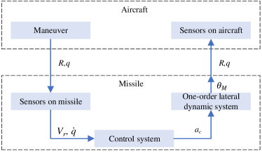
In (1), the directly accessible information about the aircraft include $V_{t}$, $\theta_{A}$, $R$, $q$, $\dot{q}$. Therefore, the equations can be written as:

$$V_{M}\cos(\theta_{M}-q)=f_{1}(V_{R},V_{A},\theta_{A},q)$$ (9)

$$V_{M}\sin(\theta_{M}-q)=f_{2}(\dot{q},R,V_{A},\theta_{A},q)$$ (10)

where

$$f_{1}(V_{R},V_{A},\theta_{A},q)=-V_{R}-V_{A}\cos(\theta_{A}+q)$$ (11)

$$f_{2}(\dot{q},R,V_{A},\theta_{A},q)=-\dot{q}R+V_{A}\sin(\theta_{A}+q)$$ (12)

Dividing (10) by (9) yields

$$\theta_{M}=\arctan\frac{f_{2}(\dot{q},R,V_{A},\theta_{A},q)}{f_{1}(V_{R},V_{A},\theta_{A},q)}+q$$ (13)

Substituting (13) into (9) yields

$$V_{M}=f_{1}(V_{R},V_{A},\theta_{A},q)\cos(\theta_{M}-q)+f_{2}(\dot{q},R,V_{A},\theta_{A},q)\sin(\theta_{M}-q)$$ (14)

The acceleration of the missile can be calculated according to data obtained from (13) and (14):

$$a_{M}=\frac{V_{M}}{g}\dot{\theta}_{M}+\cos\theta_{M}$$ (15)

Substituting (3) into (2) yields:

$$\tau_{M}=\frac{NV_{R,t}\dot{q}_{t}-a_{t}}{a_{t}-a_{t-1}}=\frac{NV_{R,t-1}\dot{q}_{t-1}-a_{t-1}}{a_{t-1}-a_{t-2}}=...=\frac{NV_{R,1}\dot{q}_{1}-a_{1}}{a_{1}-a_{0}}$$ (16)

where subscripts $t$, $t-1$, $t-2$, …, $1$, $0$ are discrete time instances.

Remark 1.

The analytic solutions to $N$ and $\tau_{M}$ can be directly calculated using above equations. However, it is hard to guarantee the accuracy of the required data considering the measurement noise. Therefore, the direct calculation of $N$ and $\tau_{M}$ may not work.

According to (13) to (16), the identification question can be written as:

$$[\tau_{M},N]=f(R,q,\theta_{A},V_{a},\nu)|_{(0,t)}$$ (17)

where $f$ represents a complex nonlinear mapping relationship and subscript $(0,t)$ represents that the question is related to time. Thus, the key to solving the question turns into finding the mapping relationships between the kinematic information and parameters.

III Identification Model

In this section, we firstly present the concept of IMMM, which can be applied to general multiple-output regression problems. Then, we present the structure of the parameter identification model, followed by dataset establishment.

Notation 1.

For simplicity, in the remainder of this paper, we denote the $sigmoid$, $tanh$, and $softmax$ functions in italics, as follows:

$$sigmoid(\zeta)=\frac{1}{1+e^{-\zeta}}$$

$$tanh(\zeta)=\frac{e^{\zeta}-e^{-\zeta}}{e^{-\zeta}+e^{\zeta}}$$

$$softmax(\zeta_{i})=\frac{e^{\zeta_{i}}}{\sum_{j}e^{\zeta_{j}}}$$

III-A Improved Multiple-Model Mechanism

The multiple-model mechanism was proposed by Wang et al. in [22]. The main idea of MMM is that use regimes to represent different possible situations by connecting a multiple-model layer behind a conventional neural network. However, the conventional MMM can only be used in single-output problems. To solve this drawback, we introduce the thought of transfer learning to MMM and propose an output processing method called the improved multiple-model mechanism.

The main idea of the IMMM is to set several groups of regimes in the multiple-model layer, with each group corresponding to a regression result of the neural network. Regimes in different groups represent possible situations of different regression results. A certain regresssion result is the weighted sum of regimes in the corresponding group.

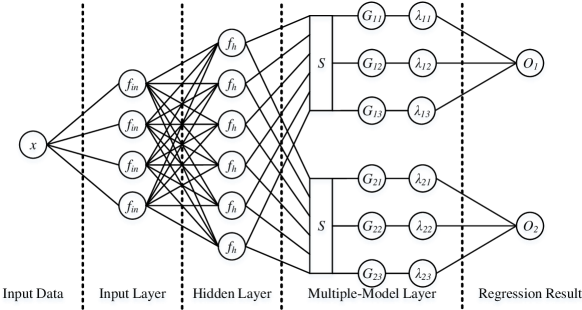
The structure of a neural network using the IMMM is shown in Figure 3. There are three types of layers: an input layer, several hidden layers and a multiple-model layer. The input layer is used to process the input data onto an appropriate range. General activation functions of the input layer include $sigmoid$ and $tanh$, whose output ranges are $[0.0,1.0]$ and $[-1.0,1.0]$, respectively. Hidden layers are the main part of the neural network, which are composed of different kinds of neurons to extract features from samples. The multiple-model layer is the main difference between a conventional neural network and a neural network using the IMMM. Regimes representing different situations are set in the multiple-model layer, and weights of different regimes are calculated through the $softmax$ function as follows:

$$G_{i}=[G_{i,1},G_{i,2},G_{i,p_{i}}]^{T}=softmax(w_{out}h_{last}+b_{out}),\sum_{j=1}^{p_{i}}G_{i,j}=1$$ (18)

where $G_{ij}$ is the $j$th regime’s weight of the $i$th regression result; $p_{i}$ is the number of regime of the $i$th regression result; $w_{out}$ is the weight matrix between the last hidden layer and the multiple-model layer; $h_{last}$ is the output of the last hidden layer; and $b_{out}$ is the bias vector. There is more than one group of regimes. Each group of regimes corresponds to a regression result, and the sum of a group of regimes is 1.

Figure 3: Improved multiple-model mechanism in the multiple-output problem.

Remark 2.

The connection between the last hidden layer and the multiple-model layer is separated into several groups instead of a full connection.

Regression results of the neural network using IMMM are the weighted sum of the corresponding group of regimes:

$$O_{i}=\Lambda_{i}^{T}G_{i}=\sum_{j=1}^{p_{i}}\lambda_{i,j}G_{i,j}$$ (19)

where $O_{i}$ is the $i$th regression result and $\lambda_{i,j}$ is the $j$th regime of the $i$th regression result.

Compared with those of a conventional neural network, the training speed and the accuracy of a neural network using IMMM is increased because the initial output ranges of the latter are limited in a required range before training, as shown in (19). Moveover, the useage of IMMM can ensure the outputs of the neural network lie within a reasonbale range, which increases the robustness of the system.

Remark 3.

The principle of transfer learning shows that the front layers of a neural network are generally used to extract primary features, while the posterior layers are used to deeply analyze samples. Therefore, the model in one problem can be used in other similar problems by merely training its last layer. The IMMM is based on this idea. Only the output of the last hidden layer is used to calculate the weights of regimes.

III-B Structure of the Parameter Identification Model

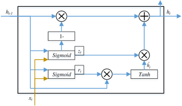
The parameter identification model established in this paper is based on the GRU neural network using IMMM . The diagram of a basic GRU neuron is shown in Figure 4, which is composed of four parts: a reset gate ($r_{t}$), an updata gate ($z_{t}$), a candidate state ($\widetilde{h}_{t}$) and an output state ($h_{t}$).

Figure 4: Basic GRU neuron.

Calculation equations of a GRU neuron are as follows:

$$r_{t}=sigmoid(w_{hr}\bullet h_{t-1}+w_{xr}\bullet x_{t}+b_{r})$$ (20)

$$z_{t}=sigmoid(w_{hz}\bullet h_{t-1}+w_{xz}\bullet x_{t}+b_{z})$$ (21)

$$\widetilde{h}_{t}=tanh(w_{h\widetilde{h}_{t}}\bullet r_{t}\times h_{t-1}+w_{x\widetilde{h}}\bullet x_{t}+b_{\widetilde{h}})$$ (22)

$$h_{t}=(1-z_{t})\times h_{t-1}+z_{t}\times\widetilde{h}_{t}$$ (23)

where $w$ is the weight matrix; $b$ is the bias vector; $\bullet$ denotes a matrix multiplication; and $\times$ denotes an element-wise multiplication. As can be seen from (20) to (23), the value of $z_{t}$ signifies the reliance on the previous information. A larger value corresponds to a smaller weight of the newly-inputting information.

The structure of the parameter identification model based on the GRU neural network using IMMM is shown in Figure 5, where each subscript $t\in N$ represents a specific time; $I_{t}$ is inputs of the model; $G_{i,j}$ is the $j$th regime’s weight of the $i$th parameter, where $i=1,2$ denote the guidance law parameter $N$ and the first-order lateral time constant $\tau_{M}$, respectively; and $\lambda_{i,j}$ is the $j$th regime of the $i$th parameter.

Figure 5: Structure of the identification model.

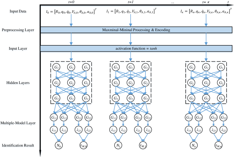
Inputs of the parameter identification are available kinematic information between the aircraft and the missile, including

$$I_{t}=[R_{t},q_{t},\dot{q}_{t},V_{A,t},\theta_{A,t},a_{A,t}]^{T}$$ (24)

The preprocessing layer is used to process and encode the input data. The input step $l$ is set according to the preset input step of model $K$ and the length of the input period $\kappa$:

$$l=\min(K,\kappa)$$ (25)

$$x_{1},x_{2},...,x_{l}=\left\{\begin{array}[]{lr}I_{1},I_{2},...,I_{\kappa},\kappa<K\\ I_{\kappa-K+1},I_{\kappa-K+2},...,I_{\kappa},\kappa\geq K\end{array}\right.$$ (26)

The input data is normalized into dimensionless values with the same range using min-max normalization:

$$\zeta(i)=\frac{\zeta^{\prime}(i)-I(i)_{min}}{I(i)_{max}-I(i)_{min}}$$ (27)

where $\zeta(i)$ is the processed data; $\zeta^{\prime}(i)$ is the initial data; $I(i)_{min}$ is the minimum value of the $i$th input data; and $I(i)_{max}$ is the maximum value of the $i$th input data.

The activation function of the input layer is $tanh$, which is used to compress or expand the input range to $[-1,1]$ and increase the nonlinear characteristic of the model. Neurons in hidden layers are basic GRU neurons, whose structure and calculation equations are shown in Figure 4 and in (20) to (23), respectively. The multiple-model layer is built according to the structure in Figure 3. The weights of different regimes are calculated by (19). The maximum and minimum regimes of each group are set as the maximum and minimum values of corresponding data in the training dataset respectively. Outputs of the model are identification results of the guidance law parameter $N$ and the first-order lateral time constant $\tau_{M}$.

III-C Dataset Establishment

The dataset is built based on the nonlinear dynamic model in subsection II-A using Latin hypercube sampling. Compared with the Monte Carlo simulation, Latin hyper sampling can increase the generalization ability of the dataset. Samples are extracted from engagement simulations using slipping windows. Inputs of the samples are shown in (24), while labels are identical to the outputs of the model. In addition, the labels are processed into the same range using max-min normalization.

Remark 4.

The Latin hypercube sampling is used twice in the process of building the dataset. It is firstly used to set the initial parameters of engagements and subsequently used to extract samples from the engagement simulations.

IV Performance Analysis

In this section, the effectiveness of IMMM and the performance of the established parameter identification model are verified by numerical simulations. We firstly present simulation parameters and engagement scenarios. Secondly, the training comparison between a conventional identification model and an identification model with IMMM is present Then, we present an sample identification run and several Monte Carlo simulations to demonstrate the performance of the established identification model. The identification accuracies under different drag coefficients are presented at the end of this section.

IV-A Simulation Parameters and Scenarios

Remark 5.

For both dataset establishment and following simulations, the simulation parameters and engagement scenarios are set in identical manners as follows.

The initial distance and LOS angle between the missile and the aircraft are $R(0)\in[6000,8000]$ and $q(0)\in[0,5]\deg$, respectively. The aircraft performs a bang-bang maneuver during the engagement, with a first-order lateral time constant $\tau_{A}=0.6s$, an initial velocity angle $\theta_{A}=0\deg$, and a constant velocity $V_{A}\in[0.8,1.0]Ma$, where $Ma=340m/s$ is the velocity of sound. The amplitude and the frequency of the bang-bang maneuver are $\eta=8g$ and $\xi=1/8$, respectively.

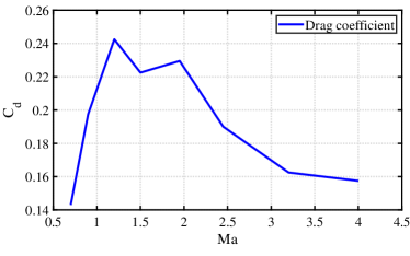
The missile is launched at $t=0$, with an initial velocity $V_{M}(0)\in[2.0,2.5]Ma$, an initial velocity angle $\theta_{M}(0)=0\deg$, and a reference area $S=0.101m^{2}$. The drag coefficient of the missile is shown in Figure 6. The guidance law parameter and the first-order lateral time constant of the missile are $N\in[2.5,5.5]$ and $\tau_{M}\in[0.1,0.4]$, respectively.

Figure 6: Drag coefficient.

The measurement sampling rate of the aircraft’s radar is $f_{m}=100Hz$. The measurement noises are $\sigma_{R}=5m$ and $\sigma_{q}=1mrad$. The simulations are performed on TensorFlow-1.13.0, and the graphic card is GeForce RTX 3090. The batch size and the number of training iterations are set as 3000 and 100000, respectively. The initial learning rate is 0.002. The dacay rate of the learning rate is 0.99/100.

IV-B Performance of IMMM

Remark 6.

The inputs of the samples used for training are not contaminated by noise.

The training comparison between a conventional identification model and an identification model with IMMM is present in this subsection. The structure of the former model is built based on the conventional model presented in [CJA]. The number of hidden layers is 3, with each hidden layer containing 96 basic GRU neurons. The preset input time length is 1s. The loss function of both models is mean square error (MSE). Models in the multiple-model layer are

$$\Lambda_{1}=[2.50,3.25,4.00,4.75,5.50]^{T}$$ (28)

$$\Lambda_{2}=[0.100,0.175,0.250,0.325,0.400]^{T}$$ (29)

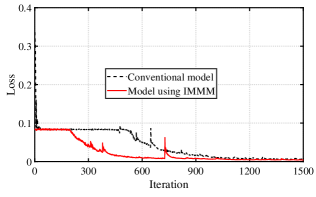
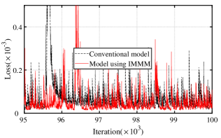
The training process is present in Figure 7 and Table I. Note that compared with that of the conventional identification model, the initial MSE of the model using IMMM reduces from 0.3366 to 0.0834. This can be explained by the fact that the initial output ranges of the model using IMMM are limited in the required range before training, as shown in (19). It can also be found that the MSE after training of the model using IMMM is lower than that of the conventional identification model, which means that the former model has a higher accuracy. This phenomenon validates the theoretical analysis in subsection III-A.

(a) The beginning of the training process

(b) The end of the training process

Figure 7: Training comparsion between the conventional model and the model using IMMM

TABLE I: MSE of the conventional model and the model using IMMM.

Model	Initial MSE	MSE after training ($\times 10^{-5}$)
Conventional Model	0.3366	10.5
Model using IMMM	0.0834	5.16

IV-C Sample Run

To intuitively demonstrate the performance of the established parameter identification model, a sample example run is presented in this subsection before turning to statistical Monte Carlo simulations. The initial distance and initial LOS angle for the sample run are $R(0)=7000m$ and $q(0)=0\deg$, respectively. The constant velocity of the aircraft is $V_{A}=0.9Ma$. The guidance law parameter and the first-order lateral time constant of the missile are $N=5.0$ and $\tau_{M}=0.30$, respectively.

(a) Weights of PN regimes

(b) Identification result of the PN parameter

(c) Weights of $\tau_{M}$ regimes

(d) Identification result of $\tau_{M}$

Figure 8: Transition process of the parameter identification model during the sample run.

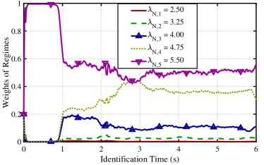
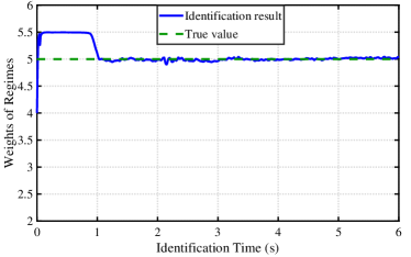
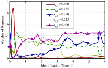
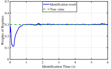
The transition process of weights of different regimes and the identification results of the model are presented in Figure 8. The weights of different regimes are identical at the beginning of the simulation; thus, the initial identification results for $N$ and $\tau_{M}$ are 4.0 and 0.25, respectively. It can be found that identification results of both the guidance law parameter and the first-order lateral time constant converge after 1 second. Then the outpus of the model fluctuate near the true value, which verifies the accuracy and the stability of the parameter identification model.

Note that in IMMM, the weights of regimes change constantly during the simulation, while the weighted sum of them, i.e., the identification results, remain stable. This is different from IMM or MMAE, in which the weight of the true situation converges to nearly $100\%$ at the end of the simualation[3, 11].

IV-D Monte Carlo Simulation

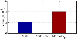
A Monte Carlo simulation with 6000 independent runs is performed to show the performance of the established identification model. In each simulation, the initial parameters are randomly set from the corresponding ranges in subsection IV-A. The samples used for the Monte Carlo simulation are extracted from trajectories that are not included in the training dataset, which can show the robustness and the generalization ability of the model. The results of the simulation are presented in Figure 9. The MSE of $N$ is $0.1158\times 10^{-3}$, while the MSE of $\tau_{M}$ is $4.0327\times 10^{-3}$. This implies that the model has a better performance in identifying the guidance law parameter.

Figure 9: Results of the Monte Carlo simulation.

An extra Monte Carlo simulation with different $N$ and $\tau_{M}$ is carried on to explore the performance of the model under different situations. The guidance law parameters are

$$N\in\{2.5,2.8,3.1,3.4,3.7,4.0,4.3,4.6,4.9,5.2,5.5\}$$

and the first-order lateral time constants are

$$\tau_{M}\in\{0.10,0.13,0.16,0.19,0.22,0.25,0.28,0.31,0.34,0.37,0.40\}$$

The other parameters are randomly set according to subsection IV-A. The number of situation is $11\times 11=121$, and the number of trajectories of each situation is 150. Randomly extracted 20 samples from each trajectory. Thus the total number of samples used for this Monte Carlo simulation is 363,000. The performances of the parameter identification model is presented in Tables II. As the tables show, the model has good performance under all conditions, which verifies the accuracy and the robustness of the parameter identification model.

TABLE II: Performance of the model under different conditions

	0.10	0.13	0.16	0.19	0.22	0.25	0.28	0.31	0.34	0.37	0.40
2.5	2.1049	2.1683	2.1378	2.1083	2.1668	2.0301	2.0728	1.8673	2.1577	2.0635	1.9578
2.8	2.0720	2.0066	2.0416	2.0121	2.1872	2.1645	2.2958	2.0286	2.1795	2.0532	2.1917
3.1	2.1323	2.3942	2.0697	1.8303	2.0843	2.0447	2.1308	1.9942	2.0125	2.1073	1.9877
3.4	2.0605	1.9035	1.7985	2.1465	1.9790	2.1042	2.1197	2.0228	2.0160	1.9873	2.1099
3.7	2.0874	2.2401	2.0292	2.0027	2.2811	2.1474	2.1627	1.9145	2.1496	2.0768	1.9666
4.0	1.9881	1.9516	1.9889	2.2014	2.0575	1.9308	2.1153	1.9723	1.9161	2.0797	2.1350
4.3	1.9425	2.0073	1.9604	2.0295	1.9342	2.1026	1.8952	2.0608	2.1089	1.8242	2.0253
4.6	2.0207	2.0896	2.1126	2.0661	2.2251	1.8649	2.1107	1.8768	2.0950	1.8525	1.8694
4.9	2.1794	2.0254	2.0687	2.1032	1.8923	2.0192	2.1390	2.0725	2.1583	2.0566	2.0050
5.2	1.9426	1.9433	1.7845	2.1938	2.0058	2.0076	2.0492	2.0246	1.9205	2.0895	1.8758
5.5	2.2283	1.9098	2.1503	2.0412	2.0574	2.1043	2.1809	1.9562	2.0670	1.9620	2.2153

IV-E Influence of the Drag Coefficient

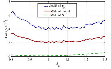
In this subsection, we present the performance of the model under different drag coefficients $C_{d}$. We enlarge or narrow the drag coefficient $\delta_{d}$ times and perform a 300-run Monte Carlo simulation for each condition. The changes of MSE are shown in Figure 10. The figure shows that the identification accuracy of the model decreases with the deviation of the drag coefficient, and the influence of $\delta_{d}$ on the identification performance of $\tau_{M}$ is larger than that of $N$. This result occurs because the first-order lateral time constant $\tau_{M}$ is generally associated with drag coefficient $C_{d}$, so it is more sensitive to deviations in $C_{d}$.

Figure 10: MSE related to $\delta_{d}$.

V Conclusion

In this paper, a regression parameter identification model based on the gated neural network is established. The inputs of the model are available information between a aircraft and a missile, while the outputs are the guidance law parameter and the first-order lateral time constant. Numerical simulations verify the performance of the model and show that the guidance law parameter has a higher identification accuracy than the first-order lateral time constant.

To increase the training speed and the accuracy of the model, thought of transfer learning is introduced to MMM and an output processing method called improved multiple-model mechanism is proposed in this paper, which can be applied to general multiple-output regression problems. The main idea of IMMM is to set several groups of regimes in the multiple-model layer, with each group corresponding to a regression result of the neural network. A certain regression result is the weighted sum of regimes in the corresponding group. Simulation results show that compared with a conventional model, the model using IMMM has a faster training speed and a higher identification accuracy. Moreover, the model using IMMM can ensure the outputs of the model lie within a reasonable range.

References

- [1] J. Speyer, “An adaptive terminal guidance scheme based on an exponential cost criterion with application to homing missile guidance,” IEEE Trans. Autom. Control, vol. 21, no. 3, pp. 371–375, Jun. 1976.
- [2] E. J. Ohlmeyer, “Root-mean-square miss distance of proportional navigation missile against sinusoidal target,” J. Guid. Control Dyn., vol. 19, no. 3, pp. 563–568, Jul. 1996. [Online]. Available: https://doi.org/10.2514/3.21658
- [3] V. Shaferman and T. Shima, “Cooperative multiple-model adaptive guidance for an aircraft defending missile,” J. Guid. Control Dyn., vol. 33, no. 6, pp. 1801–1813, Nov. 2010. [Online]. Available: https://doi.org/10.2514/1.49515
- [4] E. Garcia, D. W. Casbeer, Z. E. Fuchs and M. Pachter, “Cooperative Missile Guidance for Active Defense of Air Vehicles,” IEEE Trans. Aerosp. Electron. Syst., vol. 54, no. 2, pp. 706–721, Apr. 2018.
- [5] X. Zou, D. Zhou, R. Du, and J. Liu, “Active defense guidance law via cooperative identification and estimation,” J. Guid. Control Dyn., vol. 41, no. 11, pp. 2507–2512, Nov. 2018. [Online]. Available: https://doi.org/10.2514/1.G003372
- [6] J. Karelahti and K. Virtanen, “Adaptive controller for the avoidance of an unknownly guided air combat missile,” in 2007 46th IEEE Conf. Decision and Control, pp. 1306–1313, 2007.
- [7] R. E. Kalman, “Contribution to the theory of optimal control,” Bol. Soc. Mexicana, vol. 5, no. 63, pp. 102–119, 1960.
- [8] ——, “A new approach to linear filtering and prediction problems,” J. Basic Eng., vol. 82D, pp. 35–45, 1960.
- [9] R. E. Kalman and R. Bucy, “New results in linear filtering and prediction theory,” J. Basic Eng., vol. 83, pp. 95–108, Mar. 1961.
- [10] R. Fonod and T. Shima, “Wingman-Based Estimation and Guidance for a Sensorless PN-Guided Pursuer,” IEEE Trans. Aerosp. Electron. Syst., vol. 56, no. 3, pp. 1754–1766, Jun. 2020.
- [11] S. Li and H. Fang, “Aircraft guidance law identification using interactive multiple model estimation,” in 2018 Chinese Control And Decision Conf. (CCDC), 2018, pp. 3094–3099.
- [12] F. Lewis, Optimal estimation with an introduction to stochastic control theory. Optimal estimation with an introduction to stochastic control theory, 1988.
- [13] X. Wang, Y. Cai, Z. Yu, Q. Lin, Y. Xigui, and D. Fangxu, “Nonlinear MMAE-based missile guidance law and parameter identification,” Flighe Dyn., vol. 33, no. 5, pp. 430–434, 2015.
- [14] J. Yun and C.-K. Ryoo, “Missile guidance law estimation using modified interactive multiple model filter,” J. Guid. Control Dyn., vol. 37, no. 2, pp. 484–496, Mar–Apr 2014, AIAA Guidance, Navigation, and Control Conference, Toronto, CANADA, Aug. 02–06, 2010.
- [15] D. Magill, “Optimal adaptive estimation of sampled stochastic processes,” IEEE Trans. Autom. Control, vol. 10, no. 4, pp. 434–439, 1965.
- [16] X. R. Li, Y. Zhang, and X. Zhi, “Multiple-model estimation with variable structure. IV. design and evaluation of model-group switching algorithm,” IEEE Trans. Aerosp. Electron. Syst., vol. 35, no. 1, pp. 242–254, 1999.
- [17] S. Hochreiter and J. Schmidhuber, “Long short-term memory,” Neural Comput., vol. 9, no. 8, pp. 1735–1780, 1997.
- [18] S. K. Ibrahim, A. Ahmed, M. A. E. Zeidan, and I. E. Ziedan, “Machine Learning Methods for Spacecraft Telemetry Mining,” IEEE Trans. Aerosp. Electron. Syst., vol. 55, no. 4, pp. 1816–1827, 2019.
- [19] P. Liu, Y. Liu, T. Huang, Y. Lu, and X. Wang, “Decentralized Automotive Radar Spectrum Allocation to Avoid Mutual Interference Using Reinforcement Learning,” IEEE Trans. Aerosp. Electron. Syst., vol. 57, no. 1, pp. 190–205, 2021.
- [20] G. Cruz, and A. Bernardino, “Learning Temporal Features for Detection on Maritime Airborne Video Sequences Using Convolutional LSTM,” IEEE Trans. Aerosp. Electron. Syst., vol. 57, no. 9, pp. 6565–5476, 2019.
- [21] Y. Wang, S. Fan, G. Wu, J. Wang, and S. He, “Fast guidance law identification approach for incoming missile based on GRU network,” Acta Aeronautica et Astronautica Sinica, [Online]. Available: http://hkxb.buaa.edu.cn/CN/abstract/article_18409.shtml
- [22] Y. Wang, S. Fan, J. Wang, and S. He, “Quick identification of guidance law for an incoming missile using Multiple-Model Mechanism,” Chinese Journal of Aeronautics, [Online].
- [23] K. Cho, B. van Merriënboer, C. Gulcehre, D. Bahdanau, F. Bougares, H. Schwenk, and Y. Bengio, “Learning phrase representations using RNN Encoder–Decoder for statistical machine translation,” in Proc. 2014 Conf. Empirical Methods in Natural Language Processing (EMNLP). Doha, Qatar: Association for Computational Linguistics, Oct. 2014, pp. 1724–1734. [Online]. Available: https://www.aclweb.org/anthology/D14-1179