DataMUX: Data Multiplexing for Neural Networks

Abstract

In this paper, we introduce data multiplexing (DataMUX), a technique that enables deep neural networks to process multiple inputs simultaneously using a single compact representation. DataMUX demonstrates that neural networks are capable of generating accurate predictions over mixtures of inputs, resulting in increased inference throughput with minimal extra memory requirements. Our approach uses two key components – 1) a multiplexing layer that performs a fixed linear transformation to each input before combining them to create a ‘mixed’ representation of the same size as a single input, which is then processed by the base network, and 2) a demultiplexing layer that converts the base network’s output back into independent representations before producing predictions for each input. We show the viability of DataMUX for different architectures (Transformers, and to a much lesser extent MLPs and CNNs) across six different tasks spanning sentence classification, named entity recognition and image classification. For instance, DataMUX for Transformers can multiplex up to 20x/40x inputs, achieving up to 11x/18x increase in inference throughput with absolute performance drops of $<2\%$ and $<4\%$ respectively compared to a vanilla Transformer on MNLI, a natural language inference task. We also provide a theoretical construction for multiplexing in self-attention networks and analyze the effect of various design elements in DataMUX.

1 Introduction

Deep neural networks are very effective at modeling complex functions from real-valued vector inputs to vector outputs. However, recent studies have hinted that modern networks are vastly overparameterized Kaplan et al. (2020); Allen-Zhu et al. (2019a) and only require a fraction of their parameters for capturing many functions Frankle and Carbin (2018); Frankle et al. (2020). This raises a natural question: if networks contain greater processing capacity than necessary, could it be possible for them to model a function over multiple inputs simultaneously, similar to how radio channels share bandwidth to carry multiple information streams at once? Such a capability could enable significant improvements in efficiency and inference throughput without requiring substantial increases in model size or computation.

Figure 1: Schematic illustrating our proposed DataMUX technique in comparison to traditional minibatch processing in neural networks. Here, DataMUX uses a multiplexing layer (MUX), to multiplex $40$ instances into a single representation, passing only $32$ inputs to the neural network. The demultiplexing layer (DEMUX) uses the output to generate predictions for all $1280$ instances.

In this paper, we propose Data Multiplexing (DataMUX), a technique that enables neural networks to process multiple inputs simultaneously as a single “mixed” representation of the same size as a single input, during both training and inference (Figure 1). This is complementary to and different from minibatch processing that adds an extra batch dimension to the input, which in effect increases computational and memory requirements. Due to the use of a single combined representation, DataMUX can increase network inference throughput with minimal time and memory overhead.

The key challenge for DataMUX lies in effectively compressing a mixture of signals so that it can be processed by a neural network without sacrificing task performance. To this end, our procedure involves the addition of a multiplexing layer and a demultiplexing layer to both ends of a vanilla neural network. The multiplexing layer applies a fixed linear transformation to each input before combining them to create a single “mixed” representation. This is then fed into the base network, which processes it to obtain a “mixed” vector representation. The demultiplexing layer then converts this vector back into a set of vector representations corresponding to each original input, which is then used to make final predictions for each instance. Our multiplexing and demultiplexing layers are end-to-end differentiable, which allows us to train the entire model jointly through standard gradient descent methods. We find that training time to convergence increases almost linearly with the number of multiplexed in stances as training gets more challenging since the model has to make multiple simultaneous predictions. In order to train multiplexed models effectively, we also introduce a special token retrieval task as a pre-training objective.

We demonstrate the effectiveness of our DataMUX approach using three different architectures (Transformers Vaswani et al. (2017), MLPs, and CNNs) on six tasks spanning sentence classification, named entity recognition and image classification. Our results demonstrate that DataMUX models can successfully process between 2-40 input instances simultaneously, with minimal losses in task performance. For instance, on the sentiment analysis dataset SST-2, our multiplexed Transformer (T-MUX) can handle 40x inputs with only a $2\%$ drop in accuracy compared to a vanilla Transformer. To our best knowledge, this is the first demonstration of large-scale data multiplexing in Transformers. While our results on CNNs and MLPs for image classification are not as strong as those on Transformers, we present them to demonstrate the generality of our method and believe that better multiplexing methods may yet improve them in the future.

We further perform theoretical and empirical analyses to better understand our results. First, we show that it is possible to theoretically construct self-attention networks that can simultaneously process inputs in $N$ independent subspaces. Next, we perform several analyses of various multiplexing strategies and the effect of attention heads and model size. Finally, we also measure throughput statistics to demonstrate the efficiency gains provided by DataMUX (up to 18x inference speedup). We believe multiplexing holds great promise in improving the efficiency and versatility of neural networks and hope that future research can develop improved strategies for DataMUX and expand its applicability to more architectures and tasks.

2 Related Work

Multiplexing in deep learning

While multiplexing is a standard idea in signal processing  Rabiner and Gold (1975), its use in deep learning has been limited. Lu et al. (2020) develop MUXConv, a layer that multiplexes both spatial and channel information for convolutional neural networks (CNNs). Instead of performing data multiplexing, these models multiplex different features within the network and only process one input at a time. mixup Zhang et al. (2018) proposes a training scheme where networks are trained with a convex combination of instances to predict the instances’ label distributions from this combined representation. They find that this scheme provides implicit regularization of models and improves generalization during inference. Unlike our work however, mixup does not preserve the order of the combined instances and therefore mixed instances may not be used during inference. Another line of work uses multiple-input multiple-output training to obtain multiple sub-networks within a neural network for a relatively small number of inputs Havasi et al. (2021); Ramé et al. (2021); Soflaei et al. (2020). These approaches aim to improve single-instance performance through ensembling sub-networks’ predictions. In contrast, we are motivated by achieving optimal performance for prediction on multiple inputs and improving model throughput during inference.

Multiplexing in the brain

On the biological side, several studies hint at the capability of the brain to multiplex and transmit tremendous amounts of information with a single neural code and process them in parallel  Blumhagen et al. (2011); Akam and Kullmann (2014); Pirschel and Kretzberg (2016); Hong et al. (2016); Friedrich et al. (2004). Recently, Lankarany et al. (2019) confirmed that neurons in the somatosensory cortex multiplex different types of features (low-contrast, high-contrast) using their timing and rate of synchronous and asynchronous spiking. Rezaei et al. (2021) further provide a computational model to explain multiplexing with an ensemble of homogeneous cortical neurons. These studies increasingly demonstrate that data multiplexing is a key feature of natural neural networks.

Over-paramaterization in neural networks

Our work also relates to the over-parameterization of deep neural networks that has been investigated in several pieces of prior work Allen-Zhu et al. (2019b, a); Radhakrishnan et al. (2020). The lottery ticket hypothesis Frankle and Carbin (2018); Frankle et al. (2020); Malach et al. (2020) demonstrated that only a fraction of neurons in a trained deep model are sufficient to capture a required function. Neural architecture search Zoph and Le (2016); Liu et al. (2018); Elsken et al. (2019) aims to balance performance with parameter efficiency, by discovering the most optimal architectures for each task. There have also been several efforts at leveraging this over-parameterization effect for multi-task learning Hu and Singh (2021). Cheung et al. (2019) propose a method to superpose many models for different tasks into a single neural network, and show that it helps mitigate catastrophic forgetting. Wortsman et al. (2020) is another work along the same lines which uses a base network, along with specialized sub-networks for different tasks. Similar to these paradigms, our work possibly takes advantage of the over-parameterization existing in deep neural networks. However, to our knowledge, we are the first to utilize data multiplexing to simultaneously process multiple inputs during both training and inference, and are able to show that a fixed set of parameters can process a mixture of inputs (even up to 40) with minimal loss in accuracy.

3 Method

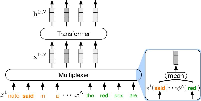
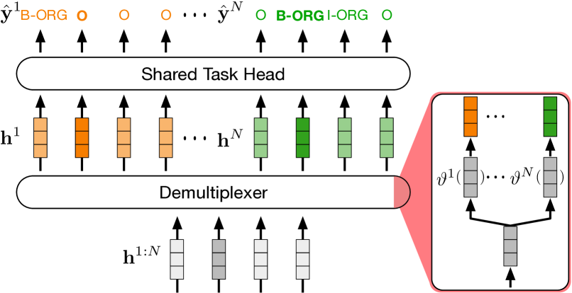
Our primary goal is to process a set of input instances simultaneously over a shared neural network (multiplexing) with minimal overhead during inference. To this end, we design DataMUX to consist of three components: a multiplexer module to combine the multiple input instances into a superposed representation, a neural network backbone to process mixed representations, and a demultiplexing module to disentangle the processed representations for individual prediction. A schematic illustrating the flow of representations is shown in Figure 2. We detail the general requirements for each component below, as well as specific implementation details used in our experiments.

3.1 Multiplexing

The multiplexer module, denoted $\Phi$, combines a tuple of inputs, either images or sentences from a batch, $(\mathbf{x}^{1},\dots,\mathbf{x}^{N})$, for $\mathbf{x}^{i}\in\mathbb{R}^{d}$, into a more compact representation $\mathbf{x}^{1:N}\in\mathbb{R}^{d}$ in an order-dependent way, which enables effective demultiplexing after processing, as well as distinguishing intra-sequence interactions in the case of sequenced inputs (e.g. token sequences). Towards this end, for each input $\mathbf{x}^{i}$ with index $i\in[1,N]$ of the input tuple, the multiplexer module performs a transformation $\phi^{i}$ ($\mathbb{R}^{d}$ $\mapsto$ $\mathbb{R}^{d}$), on the instance before finally averaging all inputs into a single multiplexed representation as:

$$\mathbf{x}^{1:N}=\Phi(\mathbf{x}^{1},\dots,\mathbf{x}^{N})=\frac{1}{N}\sum_{i=1}^{N}\phi^{i}(\mathbf{x}^{i}).$$ (1)

For sequenced inputs (e.g. token sequences), we combine $N$ sequences by multiplexing token-wise. That is for inputs of the form $\mathbf{x}^{i}=\{\mathbf{w}^{i}_{j}\}_{j\in[1,L]}$, where $\mathbf{w}^{i}_{j}\in\mathbb{R}^{d}$ is a token’s input vector representation, this operation uses the same transformation $\phi^{i}$ for each token in the sequence before averaging over each position across indices, such that $\mathbf{x}^{1:N}=\{\mathbf{w}^{1:N}_{j}\}_{j\in[1,L]}$ where $\mathbf{w}_{j}^{1:N}\in\mathbb{R}^{d}$ is a multiplexed representation of $N$ tokens at position $j$, i.e., $\mathbf{x}^{1:N}=\{\Phi(\mathbf{w}^{1}_{j},\dots,\mathbf{w}^{N}_{j})\}_{j\in[1,L]}$.

For $\phi^{i}$, we experiment with using either (1) a linear projection with a random fixed orthogonal matrix (denoted “Ortho”) or (2) the Hadamard product with a fixed Gaussian random vector (denoted “Hadmard”, equivalent to a linear map using a diagonal matrix in our case). We hope these transformations map instances at different indices into distinguishable regions and consequently reduce interference between their representations. Finally, this multiplexed representation, $\mathbf{x}^{1:N}$, is used as input to the neural network backbone, which is architecturally unchanged.

3.2 Demultiplexing

The output of the neural network backbone will be a multiplexed hidden representation $\mathbf{h}^{1:N}$ of the input $\mathbf{x}^{1:N}$. To make a prediction for each input, one can explicitly disentangle $\mathbf{h}^{1:N}$ into $N$ individual hidden representations, $\mathbf{h}^{1},\dots,\mathbf{h}^{N}$, respectively. We first obtain each $\mathbf{h}^{i}$ with a demultiplexing function $\vartheta^{i}$, i.e.,

$$\mathbf{h}^{i}=\vartheta^{i}(\mathbf{h}^{1:N}),~{}\forall i\in[1,\dots,N].$$ (2)

For sequenced input, demultiplexing is done position-wise, i.e., $\mathbf{h}^{i}_{j}=\vartheta^{i}(\mathbf{h}^{1:N}_{j})$ for each position $j$.

Finally, predictions are made using a shared task head on each inputs’ respective individual hidden representation to prevent a substantial increase in the number of parameters and improve training efficiency. We use two alternatives for the demultiplexing function $\vartheta^{i}$:

1. MLP Demuxing This strategy employs $N$ MLPs to generate each indices’ hidden representation as $\mathbf{h}^{i}=\textsc{mlp}^{i}(\mathbf{h}^{1:N})$. We use this method for both NLP and vision tasks. Although this method is conceptually simple, it adds learnable parameters proportional to $N$.

2. Index Embeddings We generate index embeddings $\mathbf{p}^{i}$, which are then concatenated to $\mathbf{h}^{1:N}_{j}$, and transformed by a shared multi-layer network to generate each individual hidden representation, i.e., $\mathbf{h}^{i}_{j}=\textsc{mlp}^{\text{shared}}(\mathbf{h}_{j}^{1:N},\mathbf{p}^{i})$. To generate the index embeddings $\mathbf{p}^{i}$, we add a sequence of $N$ special tokens, called the prefix, to the beginning of each sequence of the input tuple. For multiplexing with $N$ sequences, we add $N$ corresponding prefixes, denoted $\textit{prefix}^{i}$ for $i\in[1,N]$. Each $\textit{prefix}^{i}$ consists of a index token $\epsilon^{i}$ in it’s $i$’th position while the remaining tokens are a special pad token $\epsilon^{\text{pad}}$. The prefix sequences then take on the following pattern:

$$\textit{prefix}^{1}\hskip 3.00003pt=[\epsilon^{1},\epsilon^{\text{pad}},\ldots,\epsilon^{\text{pad}}] \textit{prefix}^{2}\hskip 3.00003pt=[\epsilon^{\text{pad}},\epsilon^{2},\epsilon^{\text{pad}},\ldots,\epsilon^{\text{pad}}] \cdots \textit{prefix}^{N}=[\epsilon^{\text{pad}},\ldots,\epsilon^{\text{pad}},\epsilon^{N}]$$

We then prepend each sequence $x^{i}$ of the input sequence with the corresponding $\textit{prefix}^{i}$. The tuple of prepended sequences is then passed to the multiplexing module. When finally generating individual hidden representations, we use the corresponding hidden representation of each index token $\epsilon^{i}$ as the index embedding $\mathbf{p}^{i}$.

We use the Index Embeddings ( 3.2) demultiplexing strategy on language tasks for the Transformer architecture. The prefix tokens may implicitly enable the Transformer to do instance-specific computations when processing the multiplexed representation and further enable demultiplexing for large $N$.

Figure 2: DataMUX for Transformers: (Left) Given a tuple of $N$ sentences ($x^{1},x^{2},\dots,x^{N}$), each of length $L$, we first apply a multiplexing operation which performs a transformation $\phi^{i}$ on the embeddings of each sequence $x^{i}$, such that the same transformation is applied to every token in a sequence $x^{i}$. The multiplexing operation then aggregates the sequences by averaging over each position, generating a single combined sequence $\mathbf{x}^{1:N}\in\mathbb{R}^{L\times d}$, for embedding size $d$, which will be passed on to the central Transformer model. (Right) After processing, we perform a demultiplexing operation to the Transformer model’s output $\mathbf{h}^{1:N}\in\mathbb{R}^{L\times d}$, to generate hidden representations $\mathbf{h}^{1},\mathbf{h}^{2},\dots,\mathbf{h}^{N}$, corresponding to inputs $x^{1},x^{2},x^{N}$ respectively. We finally use these hidden representations to generate predictions for a particular task (e.g. named entity recognition (NER)) using a shared task prediction head.

3.3 Retrieval warm-up for multiplexing

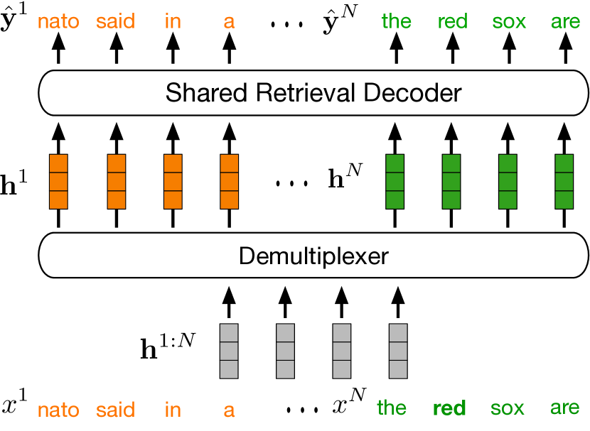
For Transformer models, we find that naively adding the multiplexing and demultiplexing layers to the model fail to converge. This is likely because the gradients for individual instances from the task loss get mixed up in the backward pass. To overcome this, we propose Retrieval warm-up – a self-supervised pre-training task to promote the ability of DataMUX models at distinguishing the order and the content of individual sequences in a multiplexed representation. This task consists of retrieving the correct tokens and order for each position and sequence of the input tuple (Figure 4). Although we could add this loss for every sentence in each position, memory constraints force us to retrieve a token from one random sentence for each token position, yielding the following objective:

$$\mathcal{L}_{\text{Retrieval}}(x^{1:N})=\sum_{j}-\log P(w^{I}_{j}|\mathbf{h}^{I}_{j}),$$ (3)

where $\mathbf{h}^{I}_{j}$ is a demultiplexed hidden representation of the $j$-th token in a randomly selected sentence with the index $I\sim\mathcal{U}[1,N]$, generated using the methods described in Section 3.2. We use this objective to optimize all the parameters of the end-to-end multiplexed model. For sequenced inputs, we find the retrieval auxiliary objective crucial to learning and report performance on the retrieval task in Section 4.2.

4 Multiplexing for Transformers (T-MUX)

4.1 Experimental setup

Models

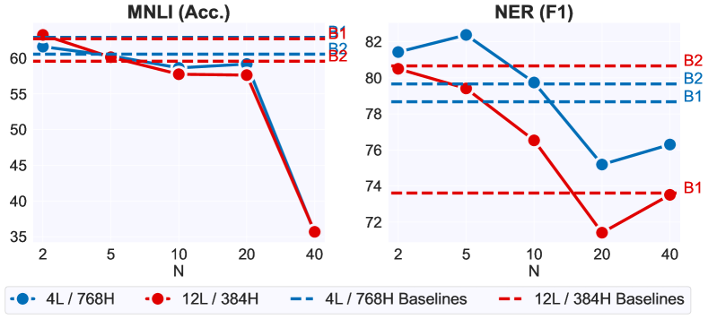
We first evaluate the capabilities and limits of data multiplexing specifically for the Transformer architecture on a range of text classification tasks. We apply DataMUX on a 12-layer Transformer based model with a hidden dimension size of 768 and 12 self-attention heads built on the Huggingface Wolf et al. (2019) framework, and refer to the resulting model as T-MUX. We compare our T-MUX models to 2 baselines: (B1) A 12-layer 768 hidden dimension vanilla Transformer. (B2) A 12-layer 768 hidden dimension Transformer pretrained using the retrieval task described in Section 3.3. Though there is no multiplexing done for B2 (meaning this operation could be solved by simply copying input tokens to the output layer) we find that the retrieval pre-training produces differences in performance and we show this baseline for completeness.

We also apply DataMUX to smaller models (see A2) and compare with similar baselines.

Tasks

We evaluate our models and the baselines on two types of text classification tasks:

1. Token-level classification: This evaluates models’ ability to perform token-level tasks on multiplexed inputs. This poses a particular challenge for data-multiplexing models since they must maintain a high level of individual token disentanglement while also producing representations capable of solving the task. We evaluate token-level classification on the CoNLL-2003 Named Entity Recognition (NER) task Sang and Meulder (2003).

2. Sentence-level classification: We evaluate models on a subset of the sentence-level classification tasks found in the General Language Understanding Evaluation (GLUE) benchmark Wang et al. (2019): the sentiment classification task SST-2 Socher et al. (2013), the sentence similarity task QQP , and the natural language inference tasks MNLI Williams et al. (2018) and QNLI Wang et al. (2019); Rajpurkar et al. (2016). By evaluating on a variety of sentence-level tasks, we can gain a better sense of the capabilities of data multiplexing neural networks on tasks that require aggregating contextual information. Similar to previous works, we prepend a [CLS] token to all sequences and learn a task head on top of the demultiplexed [CLS] token representation.

Auxiliary retrieval objective

The T-MUX models are all pre-trained using the retrieval warm-up on the Wikitext-103 dataset Merity et al. (2017) as described in Section 3.3. In addition, we also continue to use the retrieval task as an auxiliary objective during task training. The total loss is a combination of the task loss and retrieval loss (we use $\alpha=0.1$ in our experiments):

$$\mathcal{L}=(1-\alpha)\mathcal{L}_{\text{Task}}+\alpha\mathcal{L}_{\text{Retrieval}},$$ (4)

4.2 Main results

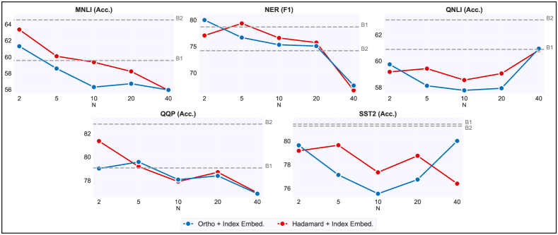
(R1) Multiplexing leads to minimal drop in performance even for large $N$

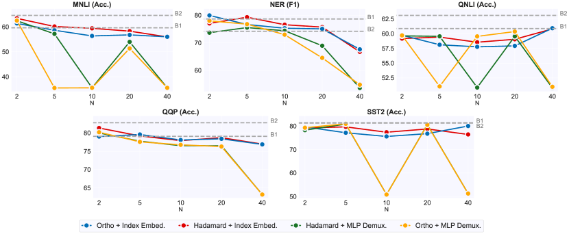
Figure 3 shows performance across four sentence classification tasks (MNLI, QNLI, QQP, SST2) and a token-level classification task (NER). We observe that it is possible to multiplex up to $40$ instances and maintain reasonable performance. For easier tasks like QQP, SST2 and QNLI, we observe that the drop in performance with increasing $N$ is insignificant while for more difficult tasks like MNLI and NER, there is a trade-off between performance and $N$, with performance dropping 10%-15% for $40$ instances. Since we’ve encountered unstable optimization when using MLP Demuxing, we only provide results using Index Embeddings demultiplexing. We find that the multiplexing strategy does not impact performance across different tasks, even slightly increasing for small values of $N$ (e.g. 2, 5). This increase may be attributable to implicit regularization à la mixup. We also did not notice much variance between fine-tuning runs and plot variance for the "Hadamard + Index Embedding" setting in Section A.4.

(R2) Perfect multiplexing on the retrieval warm-up task for large $N$

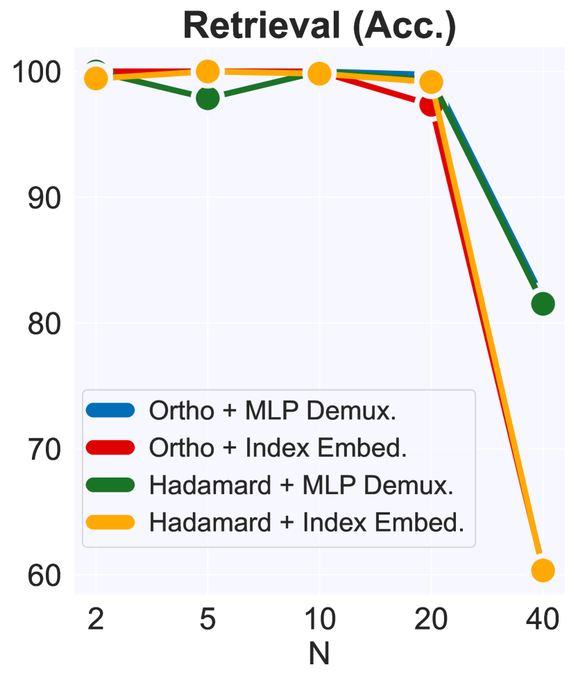
Figure  4 shows the test accuracy on the retrieval warm-up task described in Section 3.3. We first note that across different multiplexing and demultiplexing strategies, models have a retrieval accuracy of nearly $100\%$ for up to $20$ instances, demonstrating the surprising ability of T-MUX to multiplex perfectly for large $N$. Note that this task does not require any aggregation of context across the sequence and thereby is much easier than sentence classification or token-level classification tasks. Therefore, performance on this warm-up task indicates a soft upper bound on the number of instances we can multiplex for sentence and token-level classification tasks given a particular multiplexing and demultiplexing method.

Figure 3: Multiplexing task evaluation for T-MUX. Across tasks, we demonstrate multiplexing up to $40$ instances without significant drop in performance. Further, we show results here for Index Embedding demultiplexing as the MLP Demuxing method leads to optimization instability for the Transformer architecture. We provide results for the MLP Demuxing method in Appendix A.6.

Figure 4: (Left a) Given the Transformer’s combined output representation $\mathbf{h}^{1:N}$ generated from the input $(x^{1},x^{2},\dots,x^{N})$, the goal of the retrieval task is to retrieve the original tokens from $(x^{1},x^{2},\dots,x^{N})$. Since $\mathbf{h}^{1:N}$ is order-dependent, retrieval requires distinguishing not just which tokens were originally input to a position $j\in[1,L]$, but also which sentence $i\in[1,N]$ each belonged to. (Center b) Accuracy for the retrieval warm-up task. Surprisingly, models are able to retrieve words with $100\%$ accuracy up to $20$ instances across most multiplexing and demultiplexing strategies. (Right c) Runtime and throughput numbers of T-MUX models on 20K MNLI instances, normalized by a base model’s performance without multiplexing. T-MUX (12L/768H) can multiplex up to $40$ instances leading to $\sim$ $18$x speedup.

(R3) Throughput can be increased multi-fold

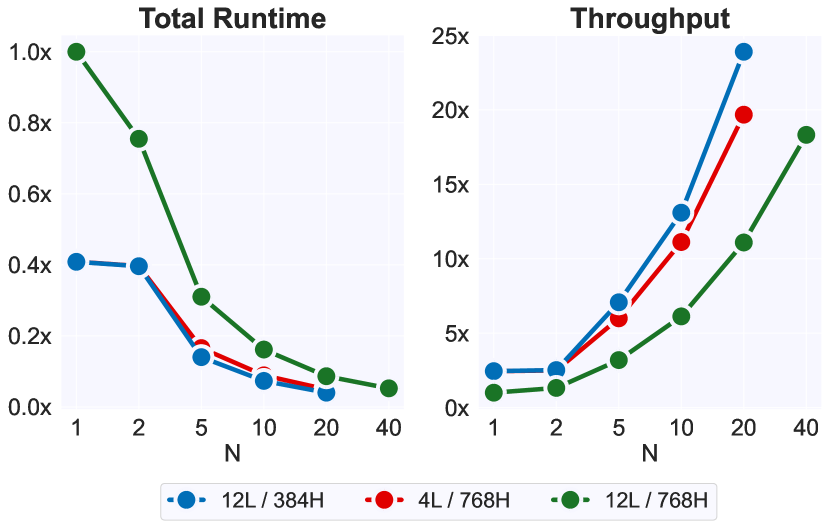
We measure throughput of our multiplexed model (Hadamard + Index Embed) across different number of instances by calculating inference speed for processing $\sim$20,000 samples on the MNLI dataset. We use four different batch sizes for all the configurations and take the max throughput (details in A.8). Figure 4 shows that multiplexing increases throughput many folds ($18$x for $40$ instances, $11$x for $20$ instances). T-MUX enables superior throughput as batch size can be effectively increased by a factor of $N$. We would expect the speedup to scale linearly with $N$, however a large $N$ corresponds to more prefix tokens which increases the sequence length. Therefore, having $40$ instances leads to almost a $20$x speedup as opposed to the expected $40$x. Future work can potentially improve this speedup by designing better multiplexing and demultiplexing strategies.

4.3 Analysis

(A1) The number of attention heads seems invariant to multiplexing

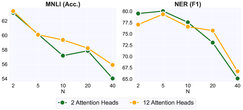
To understand the role of the number of attention heads in multiplexing, we train a variant of T-MUX with $2$ self-attention heads per layer. We use T-MUX with the (Hadamard + Index Embed.) configuration. We find that reducing self-attention heads has minimal effect on performance on the retrieval warm-up task and achieves a retrieval accuracy of $\sim 100\%$ up to $N=20$. We then find that on token and sentence-level classification tasks, T-MUX with 2 self-attention heads performs comparably to T-MUX with 12 self-attention heads (Figure 5).

Figure 5: (Left a) Understanding the role of attention heads in multiplexing. Reducing attention heads to $2$ does not impact performance greatly, suggesting that attention heads are not core to multiplexing. (Right b) Multiplexing performance with smaller model capacities. Smaller models can multiplex up to $20$ instances without significant drop in performance.

(A2) DataMUX also provides throughput boost with smaller Transformers

We further investigate the applicability of DataMUX to smaller Transformer models. We choose two smaller Transformers to multiplex: a $12$ layer with hidden size of $384$ (12L / 384H), a $4$ layer with hidden size of $768$ (4L / 768H). Figure 5 shows that these smaller T-MUX models can also multiplex up to $20$ instances with competitive performance. Figure 4 illustrates the speedup from the smaller models. As the smaller models can only multiplex up to $20$ instances with reasonable performance, we see that multiplexing with $20$ instances provides an even higher throughput of $25$x, compared to only $18$x for the full-sized T-MUX with $40$ instances.

(A3) Performance varies more across different indices as $N$ increases

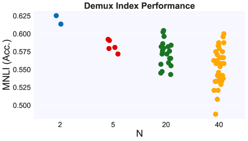
The prediction of an instance is conditioned on the index of the instance. Figure 7 illustrates performance on MNLI for different indices across different choices of $N$ for the (Hadamard + Index Embed.) configuration. We observe that performance varies more across different indices for large $N$ (For $N=40$, performance varies across $\sim 10$ percentage points).

Figure 6: T-SNE plots to understand how the demultiplexed representation of an instance changes with respect to the set of instances it is multiplexed with. Each color (10 in total) a single input sequence. Across different $N$, we find that the demultiplexed representation of an instance is not significantly impacted by the set of instances it is multiplexed with.

(A4) The demultiplexed representation of an instance is robust to the other instances it is multiplexed with

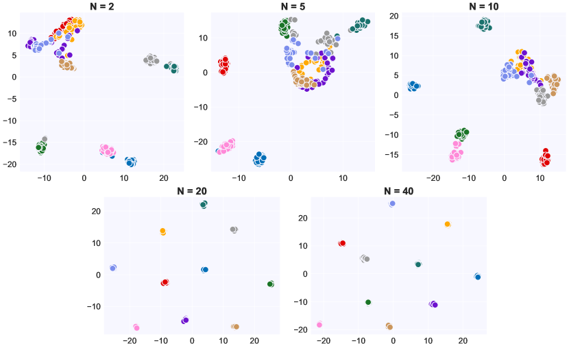
To analyze whether the representation of an instance changes with respect to the other samples it is multiplexed with, we randomly select $10$ instances $x_{1},x_{2},\cdots x_{10}$ from the MNLI dataset and multiplex each of them (separately) with $30$ different sets of other instances $y_{1}^{i},y_{2}^{i},\cdots,y_{N-1}^{i}\text{ for }i\in[1\cdots 30]$. This generates $30$ different demultiplexed representations for each of the $10$ selected samples. We then visualize the resulting points by reducing the $768$ dimensional demultiplexed representation to a $200$ dimensional vector with PCA ( F.R.S. (1901)), followed by t-SNE ( van der Maaten and Hinton (2008)) visualization. Figure 6 shows these clusters for different values of $N$. We find that across different values of $N$, all the points corresponding to the same $x_{i}$ are very close to each other, which suggests that the representation of an instance is not significantly influenced by the set of instances it is multiplexed with.

4.4 Theoretical construction for multiplexing in self-attention models

To provide some theoretical explanation for why Transformers may be amenable to multiplexing, we also detail below a construction for self-attention based neural networks which process multiplexed token embeddings in $N$ independent subspaces. Our construction relies on particular structural properties of singular spaces of linear transformations across layers – we provide a brief sketch below, with more details in Appendix A.3.

In a model with self-attention, the multi-head attention projects the queries, keys, and values $h$ times with different, learned linear projections to $d_{K}$, $d_{K}$ , and $d_{V}$ dimensions respectively. Thus, given a sequence of $d$-dimensional multiplexed token embeddings $\{\mathbf{w}_{t}^{1:N}\}_{t\in[1,L]}$, each head looks like:

Now, $\mathbf{w}^{1:N}_{t}=\frac{1}{N}\sum_{k=1}^{N}\phi^{k}(\mathbf{w}^{k}_{t})$, and let us assume each function $\phi^{k}$ can be trained to project each embedding into a subspace that is least linearly-dependent with the others. So, if we define $\mathbf{u}^{(k)}_{t}:=\frac{1}{N}\phi^{k}(\mathbf{w}^{k}_{t})$, we assume $\langle\mathbf{u}^{(k)}_{t},\mathbf{u}^{(k^{\prime})}_{t^{\prime}}\rangle\approx 0$ for all pairs of indices $k\neq k^{\prime}$ and all positions $t$. To preserve this independent subspace structure after self-attention, we will first need

This is achievable if the eigenvectors of ${\bm{W}^{V}_{i}}^{\top}\bm{W}^{V}_{i}$ can be grouped into $N$ non-overlapping subsets $\{\bm{r}^{(1)}_{1},\dots,\bm{r}^{(1)}_{m}\}$, $\cdots,$ $\{\bm{r}^{(N)}_{1},\dots,\bm{r}^{(N)}_{m}\}$, where $\bm{r}_{\ell}^{(k)}$ are orthonormal vectors (since the Gramian is real symmetric), and span the same input subspaces, denoted as $\mathcal{D}^{1},\dots,\mathcal{D}^{N}$. In this case, the vector after transformed by $\bm{W}^{V}_{i}$ can be expressed as a sum of $N$ vectors $\bm{v}_{i,t}^{(1)},\dots,\bm{v}_{i,t}^{(N)}$ in dual subspaces $\mathcal{D}_{V}^{1},\dots,\mathcal{D}_{V}^{N}$ which are independent of each other. The linear maps from $\mathcal{D}^{k}$ to $\mathcal{D}_{V}^{k}$ still allows rich operation on each component of a multiplex input without interference by other components.

In addition to decompress-able value vectors, we can set the query and key matrices, $\bm{W}_{i}^{Q}$ and $\bm{W}_{i}^{K}$, to have some subsets of right and left singular vectors such that span $\mathcal{D}^{1},\dots,\mathcal{D}^{N}$ and $\mathcal{D}^{1}_{V},\dots,\mathcal{D}^{N}_{V}$. Then, we can show that the inner product of the query and keys of the $i$-th head can be rewritten as:

$$\left(\bm{W}_{i}^{K}\mathbf{w}^{1:N}_{t^{\prime}}\right)^{\top}\bm{W}_{i}^{Q}\mathbf{w}^{1:N}_{t}=\sum_{k=1}^{N}\tau_{i,t,t^{\prime}}^{(k)},$$ (7)

where $\tau_{i,t,t^{\prime}}^{(k)}$ is a scalar only depending on the $k$-th input sequence. Thus, the self-attention operation at each position can be seen as retrieving values based on the average of query-key similarity scores of $N$ sequences.

This average retrieval using soft-max could be a desired property as implicit regularization. However, if we want perfect non-interference in retrieval, the network always has an option to specialize each head to only focus on one input sequence, by setting $\tau^{(k^{\prime})}_{i,t,t^{\prime}}=0$ for all $k^{\prime}\neq k$, which is easily achievable by controlling singular values of $\bm{W}_{i}^{Q}$ or $\bm{W}_{i}^{K}$. More details of this construction are provided in Appendix A.3. Figure 4.3 suggests that number of attention heads do not significantly impact our empirical multiplexing results. Therefore our theoretical construction does not fully explain what models learn empirically but nonetheless provides an existence proof for multiplexing under certain assumptions.

5 Multiplexing for MLPs and CNNs

We also investigate multiplexing for multilayer perceptrons (MLPs) and convolutional neural networks (CNNs). Certain cases of data multiplexing have been explored for convolutional architectures on image classification as techniques for robustness and data augmentation Ramé et al. (2021); Havasi et al. (2021); Soflaei et al. (2020). These works implicitly employed the frontend layers of a convolutional net as multiplexing layers and suggest that a convolutional neural network can learn at most 3-4 independent subnetworks concurrently Havasi et al. (2021). Since Transformers can be multiplexed for up to $40$ instances without a severe performance drop, we explore the DataMUX scheme for MLPs and CNNs on the MNIST image classification task LeCun and Cortes (2005). While our results for these architectures are not as strongly positive as for T-MUX, we believe that future work on better multiplexing strategies can make them more viable.

Figure 7: (Left a) Average test accuracy for multiplexing MLP and CNN for $N=\{1,2,4,8,16\}$ on the MNIST classification task for different multiplexing strategies. MLPs can be multiplexed up to $N=8$ without significant drop in performance while CNNs can only be multiplexed up to $4$ instances. (Right b) Performance results for different demultiplexing output indices. Results are reported for a Transformer model with the Hadamard product multiplexing and Index Embeddings demultiplexing. Variance of performance across different indices with increasing $N$.

Multiplexing for MLPs

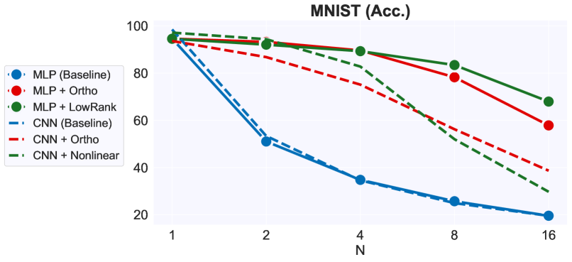
Figure 7 (solid lines) illustrates performance of DataMUX for MLPs with various multiplexing strategies, paired with the MLP demultiplexing strategy. As a baseline, we show multiplexing using the identity transformation before combining instances (MLP baseline). Since this transformation does not preserve the order of the multiplexed instances, accuracy expectedly decreases on the order of $1/N$. Multiplexing with random orthogonal matrices (MLP + Ortho) works for up to $8$ instances with an accuracy of $\sim 78\%$, compared to $\sim 95\%$ for the baseline without multiplexing. Since random orthogonal projections cannot separate inputs perfectly, we also experiment with a set of $N$ low-rank independent transformations for multiplexing (MLP + LowRank) and observe that this improves performance slightly for larger $N$ (by $5\%$ for $N$=8).

Multiplexing for CNNs

Results for CNN multiplexing are shown in Figure 7 (dashed lines). Like in the MLP case, all methods shown use the MLP demultiplexing strategy. We notice that the baselines (CNN baseline) has a roughly $N$-fold performance drop because of the unidentifiability of input order. The “Ortho” transformation performs quite poorly for CNNs (only $\sim 56\%$ for $N=8$). This is likely because this transformation destroys the property of spatial locality that CNNs rely on. We therefore also explore $N$ two-layer convolutional networks with a tanh activation as out multiplexing transformations $\phi^{i}$ (CNN + Nonlinear). We note that even with this transformation, the dimensionality of the multiplexed representation still remains equal to the dimensionality of a single input. We find that for $N\leq 4$, performance is above $80\%$, which is significantly better than CNN+Ortho, but performance drops rapidly for $N>4$. We show results of other multiplexing strategies for CNN in Appendix A.11.

Overall, multiplexing for MLPs and CNNs seems to be more challenging than Transformers as evidenced by the sharper performance drops with increasing $N$. However, we believe these numbers are still non-trivial and show the potential for multiplexing in CNNs and MLPs, with multiplexing and demultiplexing strategies better suited for these architectures.

6 Discussion

In this work, we have shown that neural networks can be trained to multiplex, i.e. process multiple inputs using a single “mixed” representation. We introduced DataMUX, a novel setting for training and inference with multiplexing, and demonstrate its viability using a variety of network architectures and tasks. Our results reveal the surprising ability of neural networks to predict on up to $40$ input instances simultaneously using data multiplexing. Our efforts have sought to show the potential for data multiplexing using methods that require limited computational overhead or added learned parameters; achieving results that incur minimal degradation in performance while simultaneously increasing system throughput dramatically.

While the scope of this paper is to demonstrate the general ability and potential for neural networks to use data multiplexing, there are several avenues for future research to investigate the limits and theoretical implications of DataMUX. Directions of particular interest include: large-scale pre-training, multi-modal processing, multi-lingual models, different mechanisms of multiplexing and demultiplexing, and a more rigorous understanding of the architectural, data, and training conditions enabling data multiplexing.

7 Acknowledgements

We thank Ameet Deshpande, Shunyu Yao, Jens Tuyls, Tianyu Gao and Mengzhou Xia for their valuable feedback on early drafts and encouragement throughout the course of this project, and the anonymous reviewers for their suggestions on improving the paper.

Checklist

1. For all authors…

   1. Do the main claims made in the abstract and introduction accurately reflect the paper’s contributions and scope? [Yes]

   2. Did you describe the limitations of your work? [Yes] Refer to A.2

   3. Did you discuss any potential negative societal impacts of your work? [Yes] Refer to A.2

   4. Have you read the ethics review guidelines and ensured that your paper conforms to them? [Yes]

2. If you are including theoretical results…

   1. Did you state the full set of assumptions of all theoretical results? [Yes]

   2. Did you include complete proofs of all theoretical results? [Yes]

3. If you ran experiments…

   1. Did you include the code, data, and instructions needed to reproduce the main experimental results (either in the supplemental material or as a URL)? [Yes] Refer to supplementary material

   2. Did you specify all the training details (e.g., data splits, hyper-parameters, how they were chosen)? [Yes] Refer to A.9 and  A.10

   3. Did you report error bars (e.g., with respect to the random seed after running experiments multiple times)? [Yes] Refer to A.4

   4. Did you include the total amount of compute and the type of resources used (e.g., type of GPUs, internal cluster, or cloud provider)? [Yes] Refer to A.8

4. If you are using existing assets (e.g., code, data, models) or curating/releasing new assets…

   1. If your work uses existing assets, did you cite the creators? [Yes]

   2. Did you mention the license of the assets? [N/A]

   3. Did you include any new assets either in the supplemental material or as a URL? [N/A]

   4. Did you discuss whether and how consent was obtained from people whose data you’re using/curating? [N/A]

   5. Did you discuss whether the data you are using/curating contains personally identifiable information or offensive content? [N/A]

5. If you used crowdsourcing or conducted research with human subjects…

   1. Did you include the full text of instructions given to participants and screenshots, if applicable? [N/A]

   2. Did you describe any potential participant risks, with links to Institutional Review Board (IRB) approvals, if applicable? [N/A]

   3. Did you include the estimated hourly wage paid to participants and the total amount spent on participant compensation? [N/A]

Appendix A Appendix

A.1 Ethical considerations

DataMUX has the potential to provide great computational efficiency when used in real production systems, where queries across different users can be aggregated to get simultaneous predictions for different users. However, this also present potential risks and scope for misuse. First, the multiplexing layer might ‘leak’ data between different users, which could potentially lead to privacy concerns. Second, the output of an instance might be influenced by other instances in the multiplexing batch, which may present the possibility of black-box attacks to manipulate information, especially in the multi-user setting. Finally, DataMUX models predictions could be harder to interpret with current techniques since the model’s internal representations depend on the set of instances it was multiplexed with.

We believe these are important and interesting research problems to solve technically and may also require careful policy development for deploying these models (e.g. restricting multiplex batches to single users).

A.2 Limitations

Here, we list some of the limitations of this work:

• Convergence time increases with increasing number of instances: Training multiplexed models with large number of instances takes larger number of iterations for convergence as increasing number of instances increases the difficulty of multiplexing and demultiplexing. We hope that future work can explore different multiplexing and demultiplexing strategies to improve rate of convergence during training.

• Multiplexing on CNNs and MLPs not as strong as that of the Transformer: While we demonstrate non-trivial multiplexing capabilities for the CNN and MLP architectures with our approach, the results are not as strong as that of the Transformer architecture. We hope future work will develop better multiplexing approaches for these architectures.

A.3 Theoretical construction of multiplexing transformer

Following the same notations defined in Section 4.4, assume that the components of a multiplexed input, $\mathbf{u}_{t}^{(1)},$ $\dots,$ $\mathbf{u}_{t}^{(N)}$, all approximately lie in $N$ linearly independent subspaces $\mathcal{D}^{1}$, $\dots$,$\mathcal{D}^{N}$. Equation 6 is realizable when eigenvectors of ${\bm{W}^{V}_{i}}^{\top}\bm{W}^{V}_{i}$ can be grouped into $N$ non-overlapping subsets $\{\bm{r}^{(1)}_{1},\dots,\bm{r}^{(1)}_{m}\}$, $\cdots,$ $\{\bm{r}^{(N)}_{1},\dots,\bm{r}^{(N)}_{m}\}$, where $\bm{r}_{\ell}^{(k)}$ are orthonormal vectors (since the Gramian is real symmetric), and span the same input subspaces. In this case, the vector after linear transformation $\bm{W}^{V}_{i}$ can be expressed as a superposition of $N$ vectors in $N$ independent subspaces $\mathcal{D}_{V}^{1},\dots,\mathcal{D}_{V}^{N}$. We now verify this statement.

Proof. Since eigenvectors of ${\bm{W}^{V}_{i}}^{\top}\bm{W}^{V}_{i}$ span the same subspaces, we can write each component of $\mathbf{w}^{1:N}_{t}$ as a linear combination of the corresponding subset of eigenvectors,

$$\mathbf{w}^{1:N}_{t}=\sum_{k}\mathbf{u}_{t}^{(k)}=\sum_{k,\ell}\alpha^{(k)}_{\ell,t}\bm{r}^{(k)}_{\ell}.$$ (9)

Let $\bm{W}^{V}_{i}=\bm{L}\bm{\Sigma}\bm{R}^{\top}$be the singular decomposition of $\bm{W}^{V}_{i}$, where $\bm{L}\in\mathbb{R}^{d_{V}\times d_{V}}$, $\bm{R}\in\mathbb{R}^{d\times d}$ are two orthogonal matrices, and $\bm{\Sigma}$ is a $d_{V}\times d$ rectangular diagonal matrix with non-negative real numbers on the diagonal. For each column of $\bm{R}$ that contributes to input subspaces, e.g., $\bm{r}_{\ell}^{(k)}$, we denote the dual left singular vector at the corresponding column of $\bm{L}$ as $\bm{l}_{\ell}^{(k)}$, and the singular value at the corresponding column and row $\sigma_{\ell}^{(k)}$

$$\bm{v}_{i,t} = \bm{W}^{V}_{i}\mathbf{w}^{1:N}_{t}=\bm{L}\bm{\Sigma}\bm{R}^{\top}\sum_{k,\ell}\alpha^{(k)}_{\ell,t}\bm{r}_{\ell}^{(k)}$$ (10)

$$= \sum_{k=1}^{N}\left(\sum_{\ell}\alpha_{\ell,t}^{(k)}\sigma_{\ell}^{(k)}\bm{l}_{\ell}^{(k)}\right).$$ (11)

Since $\bm{l}_{\ell}^{(k)}$ are columns of $\bm{L}$ that are orthogonal to each other, $\bm{v}_{i,t}$ above is a superposition of $N$ vectors $\bm{v}_{i,t}^{(k)}$ in independent subspaces, and each subspace is defined by

$$\mathcal{D}^{V}_{k}\cong{\tt span}\{\bm{l}_{\ell}^{(k)}\}.$$ (12)

$\blacksquare$

In addition to decompress-able value vectors, we can set the linear transformations for queries and keys to have the same singular space structures to prevent complicated interference. More specifically, assume that $\bm{W}_{i}^{Q}$ and $\bm{W}_{i}^{K}$ have some subsets of right and left singular vectors such that

$$\mathcal{D}_{k}\cong{\tt span}\{{\bm{r}^{Q}_{\ell}}^{(k)}\}\cong{\tt span}\{{\bm{r}^{K}_{\ell}}^{(k)}\},$$ (13)

and

$$\mathcal{D}^{K}_{k}\cong{\tt span}\{{\bm{l}^{Q}_{\ell}}^{(k)}\}\cong{\tt span}\{{\bm{l}^{K}_{\ell}}^{(k)}\}.$$ (14)

The inner product between the query and keys can be rewritten as

$$\left(\bm{W}_{i}^{K}\mathbf{w}^{1:N}_{t^{\prime}}\right)^{\top}\bm{W}_{i}^{Q}\mathbf{w}^{1:N}_{t}$$ (15)

$$=\leavevmode\resizebox{151.76964pt}{}{$\displaystyle\left(\sum_{k,\ell}\beta_{\ell,t^{\prime}}^{(k)}{\sigma^{K}_{\ell}}^{(k)}{\bm{l}_{\ell}^{K}}^{(k)}\right)^{\top}\left(\sum_{k,\ell}\gamma_{\ell,t}^{(k)}{\sigma^{Q}_{\ell}}^{(k)}{\bm{l}_{\ell}^{Q}}^{(k)}\right)$}$$ (16)

$$=\leavevmode\resizebox{151.76964pt}{}{$\displaystyle\sum_{k=1}^{N}\left[\sum_{\ell,\ell^{\prime}}\beta_{\ell^{\prime},t^{\prime}}^{(k)}\gamma_{\ell,t}^{(k)}{\sigma^{K}_{\ell^{\prime}}}^{(k)}{\sigma^{Q}_{\ell}}^{(k)}\left({\bm{l}_{\ell^{\prime}}^{K}}^{(k)}\right)^{\top}{\bm{l}_{\ell}^{Q}}^{(k)}\right]$}$$ (17)

$$=\sum_{k=1}^{N}\tau_{t,t^{\prime}}^{(k)}$$ (18)

where $\tau_{t,t^{\prime}}^{(k)}$ is a scalar only depending on the $k$-th input sequence (for simplification we omit head index $i$). Thus, the self-attention operation at each position can be seen as retrieving values based on the average of query-key similarity scores of $N$ sequences.

$$\leavevmode\resizebox{182.1196pt}{}{$\displaystyle head_{i}(t):=\sum_{t^{\prime}}\left[\frac{\exp\left(\sum_{k}\tau_{i,t,t^{\prime}}^{(k)}/\sqrt{d_{K}}\right)}{\sum_{t^{\prime\prime}}\exp\left(\sum_{k}\tau_{i,t,t^{\prime\prime}}^{(k)}/\sqrt{d_{K}}\right)}\sum_{k}\bm{v}_{i,t}^{(k)}\right]$}.$$ (19)

The average retrieval by soft-max could be undesirable. However, this will not affect the quality of decompression at all. If we want perfect non-interference in retrieval, one always has an option to specialize each head to only focus on one input sequence, by setting $\tau^{(k^{\prime})}_{i,t,t^{\prime}}=0$ for all $k^{\prime}\neq k$. This is easily achievable by controlling singular values of $\bm{W}_{i}^{Q}$ or $\bm{W}_{i}^{K}$.

Finally, we concatenate all heads and linearly project the output with $\bm{W}^{O}\in\mathbb{R}^{d\times hd_{V}}$ to a $d$-dimensional space again. This step is exactly equivalent to having $h$ projection matrices $\bm{W}^{O}_{i}\in\mathbb{R}^{d\times d_{V}}$ acting on different heads and aggregating resulting vectors.

Employing a similar structure for right singular vectors as $\bm{W}^{V}_{i}$, we can make each $\bm{W}^{O}_{i}$ also preserves the independence of subspaces.

A.4 Multiplexing with Hadamard + Ortho strategy trains consistently for different runs

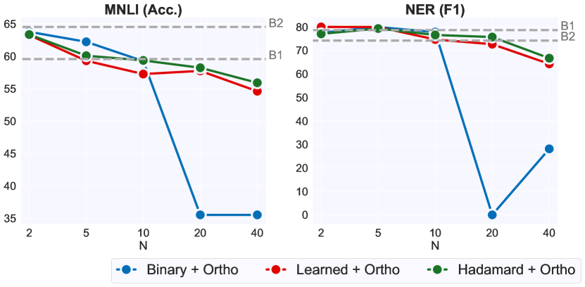
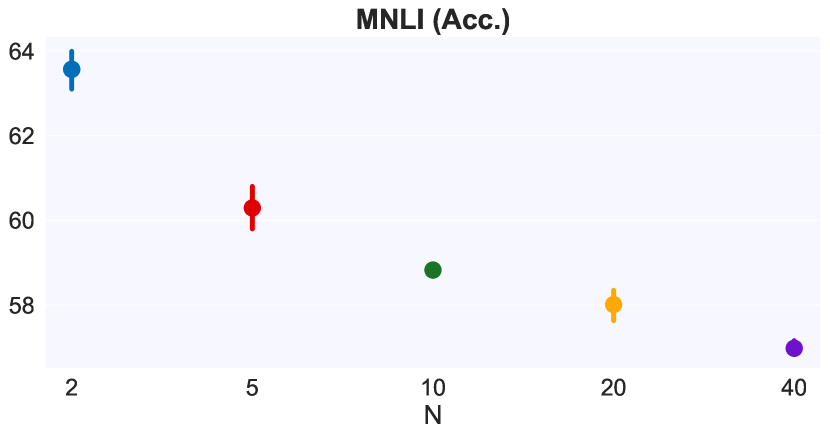
In Figure 8 we show MNLI performance for the Hadamard + Ortho multiplexing strategy with error bars across 3 random seeds. We observe that the value of $N$ has no effect on variance in performance across seeds, with all values showing minimal variance. Since we use the same retrieval pre-trained weights, the random seed only affects the demultiplexer and classification head initializations.

Figure 8: (Left a) Evaluation on alternative superposition methods for multiplexing. Binary vectors fail to multiplex beyond $10$ instances, while unfreezing Gaussian vectors for multiplexing does not help. (Right b) MNLI accuracy results with error bar for the Hadamard + Ortho strategy across 3 different random seeds. Variance in performance is minimal to none.

A.5 Alternate multiplexing strategies

We experiment with different multiplexing strategies and use index embeddings for demultiplexing. For the Hadamard product, we try unfreezing the random Gaussian vectors and update through optimization (“Learned”). We also experiment with binary masking, where the $i^{th}$ binary vector selects the $i^{th}$ chunk of size $d/N$ from the input representation of instance $i$ (“Binary”). We first look at the performance on the retrieval warm-up task. Figure 4 shows that the unfreezing the vectors does not significantly change performance. We also observe that binary vectors fails to multiplex for large $N$, suggesting the multiplexing is more capable than just concatenating multiple downsampled inputs of $d/N$ dimension when $N$ is large. We see similar trends for the MNLI and NER (illustrated in Figure 8) with unfrozen vectors not impacting performance and binary vectors failing to multiplex for large $N$.

Figure 9: Primary results for NLP tasks mirroring those shown in Figure 3. We additionally show results for the MLP Demux. strategy. While MLP Demux. demultiplexing very works well for retrieval, shown in Figure 4, we find that it typically performs slightly worse than the Index Embedding method and it leads to unstable optimization. This method also leads to an increase in parameter size proportional to $N$, since we must now train $N$ independent MLPs for each input index.

A.6 MLP Demux Results

We show our primary results for NLP tasks in Figure 3, though we’ve excluded models using the MLP Demux. demultiplexing method. We provide these results instead in Figure 9 to highlight the optimization instability encountered during training of models using the MLP Demux. method. Especially curious is the failure to converge at apparently arbitrary points for $N$, such as converging for $N=20$ for MNLI yet not converging for $N=10$ despite $N=10$ being a presumably simpler setting.

A.7 Smaller models achieve good performance across tasks

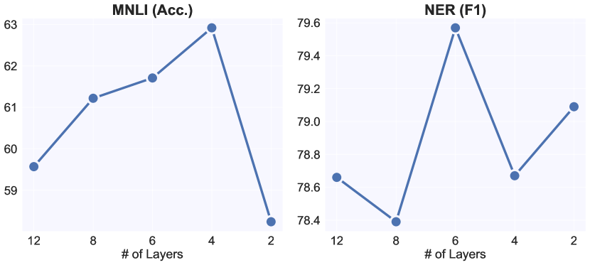
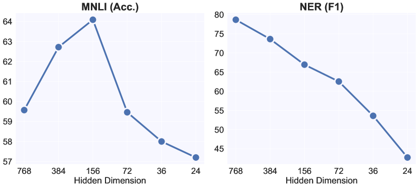
For our evaluation tasks, our base model might be over-parametrized and smaller models might perform equally well. Figures 10 shows performance on MNLI and NER as we vary the hidden size and the number of layers in the transformer. We observe that smaller models are competitive on both tasks and in the following section explore the possibility of getting higher throughput by multiplexing smaller models.

Figure 10: Model performance for different hidden dimension sizes and number of layers.

A.8 Experiment details for computing throughput

We compute throughput over $20000$ samples on the MNLI task on a single Nvidia RTX 2080 machine. We use $4$ batch sizes and take the maximum value.

A.9 Implementation details for multiplexing Transformers

We train all models to convergence. We use a learning rate of $2e-5$ and $5e-5$ for baselines and report the best performance. For multiplexed models, we use a learning rate of $5e-5$. However, for large $N$, we use $2e-5$ in case learning rate of $5e-5$ does not converge. We use a batch size of $32$ for the baselines and use slightly smaller batch sizes for multiplexing as multiplexing effectively increase our size of the batch and therefore we need to keep more input instances in memory, leading to a drop in batch size. For the language tasks, we report numbers on the validation split and do not perform any extensive hyper-parameter sweeps.

A.10 Experiment Design details for CNNs and MLPs

Each image is cropped as $20\times 20$ pixels at the center and trained with standard stochastic gradient decent. We also do not apply weight decay or other regularization as these are orthogonal to the multiplexing setting.

Principle component analysis on all $60000$ training images indicates that $86.54\%$ variance can be explained by top $50$ principle components, suggesting that if we only keep the top $50$ dimensions for each input image and project them into linearly independent subspaces, ideally we can multiplex $8(d=400/50)$ inputs as just one input without much information loss. We test the model performances with $N=\{1,2,4,8,16\}$ multiplexed inputs.

Our MLP consists of a hidden layer with 100 neurons, a demultiplexing layer that maps the 100 hidden neurons to $20\times N$ neurons, and a shared linear readout layer that maps each group of 20 neurons to 10 categories for classification. Our CNN is similar to the classic LeNet LeCun et al. (1989), consisting of three convolutional layers with 10 activation maps from 3x3 kernels, 16 activation maps from 4x4 kernels and 120 activation maps from 3x3 kernels, one linear layer maps to 84 hidden neurons, a demultiplexing layer that maps them to $84\times N$ neurons, and a shared linear readout layer that maps each group of 84 neurons to 10 categories for classification. The first two convolutional layers are followed by 2x2 max pooling. Every linear layer or convolution layer in our models is followed by a $\tanh$ activation. Labels are $+1$ for the correct digit and $-1$ for the incorrect digits. And we use the mean squared error (MSE) loss to train all our models.

We train all our models with the standard stochastic gradient decent with fixed learning rates, and the batch size is 32.

To generate the low-rank approximations (“LowRank” in Figure 7), we divide $d$ random orthogonal row vectors into $N$ groups, and multiplying them by another $d\times d$ orthogonal matrix.

A.11 Other multiplexing strategies for CNNs

To make the multiplexing method more compatible with CNNs, we first tried some simple separation functions for images. 2D rotations (SO(2)) work much better than $\text{SO}(d)$ when $N\leq 2$. When $N=1$, rotating inputs certainly does no harm to the performance. When $N=2$, there is some unavoidable interference between two rotated images, while CNN can still easily distinguish inputs with decent accuracy. However, when $N>2$, inputs are heavily overlapped, and CNN fails to distinguish many digits. The accuracy among different inputs also varies largely, with std. at 10-24% when $N\geq 8$, indicating the permutation symmetry of inputs is hard to preserve during optimization. We also tried other simple 2D transformations like mosaic and downsampling so that all inputs are perfectly separated but get blurred. CNN can only answer one of the inputs correctly for this mosaic transformation, since we are only testing the vanilla convolutional architecture, which is not suitable for object detection without proposing bounding boxes.

Figure 11: Averaged test accuracy for multiplexing CNN for $N=\{1,2,4,8,16\}$ inputs on the MNIST classification task, with different multiplexing strategies. Results are stable across multiple runs.

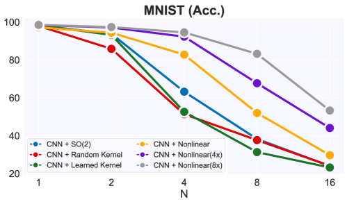
Figure 11 summarizes the performance of other separation functions we used for multiplexing CNN that can preserve spacial locality of images. During multiplexing, we can slide a 3x3 kernel over each input images before summing them up. This make CNN able to distinguish different inputs even with random initialized weights from $\mathcal{N}(0,1)$ (CNN+Random Kernel). We also make the weights of all $N$ multiplexing kernels learned but the difference is subtle (CNN+Learned Kernel), and the its performance is worse than a multiplexing CNN with 2D rotations. Also, we find that these multiplexing CNN can always answer at most two inputs correctly each time. This is because sliding a small kernel over image is a very constrained linear transformation that cannot do much to separate images, and the permutation symmetry has to be broken during the training dynamics to improve accuracy.

To increase the expressibility of separation functions while keep it compatible with CNN, we apply $N$ small convolutional nets with two layers of 16 3x3 kernels and tanh activation to input images, and sum up their activation maps (CNN+Nonlinear). A multiplexing CNN with this nonlinear separation function is similar to the MIMO approach in the previous study Ramé et al. (2021); Havasi et al. (2021), and we observe the performance changes consistent with the literature. When $N\leq 4$, its test average test accuracy is above 80%, which is also better than multiplexing CNN with $\text{SO}(d)$. However, when $N>4$, the performance drops rapidly. The accuracy across inputs becomes stabler with std. at about 7% when $N\geq 8$. If we allow higher dimensionality of the multiplexed input over a single input, that is use $4$ activation maps (CNN+Nonlinear(4x)) or 8 activation maps (CNN+Nonlinear(8x)) instead of using a single activation map, we can keep improving the accuracy for larger $N$ while still providing improved throughput.

A.12 Memory overhead for multiplexed models

Figure 12: Memory overhead of multiplexed models during inference increases linearly with increasing N, with a very gentle slope (Memory overhead for N = 40 is $\sim 4$x than N = 1).

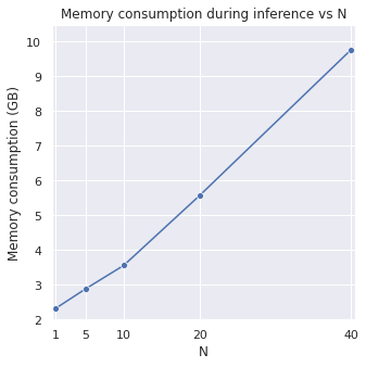
We measure the memory overhead of various multiplexed models in Figure 12. We use a fixed minibatch size of $60$ for all N and measure GPU memory during inference. We use the index demultiplexing strategy along with the Hadamard multiplexing strategy. We note that the memory increases linearly with increasing N as the number of inputs to the demultiplexing layers increases linearly with increasing N. However, the rate of growth is very gentle and the memory for N = 40 grows only by a mere $\sim 4$x compared to the baseline model.

References

- Akam and Kullmann (2014) Thomas Akam and Dimitri M Kullmann. 2014. Oscillatory multiplexing of population codes for selective communication in the mammalian brain. Nature Reviews Neuroscience, 15(2):111–122.
- Allen-Zhu et al. (2019a) Z Allen-Zhu, Y Li, and Y Liang. 2019a. Learning and generalization in overparameterized neural networks, going beyond two layers. Advances in neural information processing systems.
- Allen-Zhu et al. (2019b) Zeyuan Allen-Zhu, Yuanzhi Li, and Zhao Song. 2019b. A convergence theory for deep learning via over-parameterization. In International Conference on Machine Learning, pages 242–252. PMLR.
- Blumhagen et al. (2011) Francisca Blumhagen, Peixin Zhu, Jennifer Shum, Yan-Ping Zhang Schärer, Emre Yaksi, Karl Deisseroth, and Rainer W Friedrich. 2011. Neuronal filtering of multiplexed odour representations. Nature, 479(7374):493–498.
- Cheung et al. (2019) Brian Cheung, Alexander Terekhov, Yubei Chen, Pulkit Agrawal, and Bruno Olshausen. 2019. Superposition of many models into one. In Advances in Neural Information Processing Systems, volume 32. Curran Associates, Inc.
- Elsken et al. (2019) Thomas Elsken, Jan Hendrik Metzen, and Frank Hutter. 2019. Neural architecture search: A survey. The Journal of Machine Learning Research, 20(1):1997–2017.
- Frankle and Carbin (2018) Jonathan Frankle and Michael Carbin. 2018. The lottery ticket hypothesis: Finding sparse, trainable neural networks. arXiv preprint arXiv:1803.03635.
- Frankle et al. (2020) Jonathan Frankle, Gintare Karolina Dziugaite, Daniel Roy, and Michael Carbin. 2020. Linear mode connectivity and the lottery ticket hypothesis. In International Conference on Machine Learning, pages 3259–3269. PMLR.
- Friedrich et al. (2004) Rainer W Friedrich, Christopher J Habermann, and Gilles Laurent. 2004. Multiplexing using synchrony in the zebrafish olfactory bulb. Nature neuroscience, 7(8):862–871.
- F.R.S. (1901) Karl Pearson F.R.S. 1901. Liii. on lines and planes of closest fit to systems of points in space. The London, Edinburgh, and Dublin Philosophical Magazine and Journal of Science, 2(11):559–572.
- Havasi et al. (2021) Marton Havasi, Rodolphe Jenatton, Stanislav Fort, Jeremiah Zhe Liu, Jasper Snoek, Balaji Lakshminarayanan, Andrew Mingbo Dai, and Dustin Tran. 2021. Training independent subnetworks for robust prediction. In 9th International Conference on Learning Representations, ICLR 2021, Virtual Event, Austria, May 3-7, 2021. OpenReview.net.
- Hong et al. (2016) Sungho Hong, Mario Negrello, Marc Junker, Aleksandra Smilgin, Peter Thier, and Erik De Schutter. 2016. Multiplexed coding by cerebellar purkinje neurons. Elife, 5:e13810.
- Hu and Singh (2021) Ronghang Hu and Amanpreet Singh. 2021. Unit: Multimodal multitask learning with a unified transformer. arXiv preprint arXiv:2102.10772.
- Kaplan et al. (2020) Jared Kaplan, Sam McCandlish, Tom Henighan, Tom B Brown, Benjamin Chess, Rewon Child, Scott Gray, Alec Radford, Jeffrey Wu, and Dario Amodei. 2020. Scaling laws for neural language models. arXiv preprint arXiv:2001.08361.
- Lankarany et al. (2019) Milad Lankarany, Dhekra Al-Basha, Stéphanie Ratté, and Steven A. Prescott. 2019. Differentially synchronized spiking enables multiplexed neural coding. Proceedings of the National Academy of Sciences, 116(20):10097–10102.
- LeCun et al. (1989) Yann LeCun, Bernhard E. Boser, John S. Denker, Donnie Henderson, Richard E. Howard, Wayne E. Hubbard, and Lawrence D. Jackel. 1989. Handwritten digit recognition with a back-propagation network. In Advances in Neural Information Processing Systems 2, [NIPS Conference, Denver, Colorado, USA, November 27-30, 1989], pages 396–404. Morgan Kaufmann.
- LeCun and Cortes (2005) Yann LeCun and Corinna Cortes. 2005. The mnist database of handwritten digits.
- Liu et al. (2018) Chenxi Liu, Barret Zoph, Maxim Neumann, Jonathon Shlens, Wei Hua, Li-Jia Li, Li Fei-Fei, Alan Yuille, Jonathan Huang, and Kevin Murphy. 2018. Progressive neural architecture search. In Proceedings of the European conference on computer vision (ECCV), pages 19–34.
- Lu et al. (2020) Zhichao Lu, Kalyanmoy Deb, and Vishnu Naresh Boddeti. 2020. Muxconv: Information multiplexing in convolutional neural networks. 2020 IEEE/CVF Conference on Computer Vision and Pattern Recognition (CVPR), pages 12041–12050.
- Malach et al. (2020) Eran Malach, Gilad Yehudai, Shai Shalev-Schwartz, and Ohad Shamir. 2020. Proving the lottery ticket hypothesis: Pruning is all you need. In International Conference on Machine Learning, pages 6682–6691. PMLR.
- Merity et al. (2017) Stephen Merity, Caiming Xiong, James Bradbury, and Richard Socher. 2017. Pointer sentinel mixture models. ArXiv, abs/1609.07843.
- Pirschel and Kretzberg (2016) Friederice Pirschel and Jutta Kretzberg. 2016. Multiplexed population coding of stimulus properties by leech mechanosensory cells. Journal of Neuroscience, 36(13):3636–3647.
- Rabiner and Gold (1975) Lawrence R Rabiner and Bernard Gold. 1975. Theory and application of digital signal processing. Englewood Cliffs: Prentice-Hall.
- Radhakrishnan et al. (2020) Adityanarayanan Radhakrishnan, Mikhail Belkin, and Caroline Uhler. 2020. Overparameterized neural networks implement associative memory. Proceedings of the National Academy of Sciences, 117(44):27162–27170.
- Rajpurkar et al. (2016) Pranav Rajpurkar, Jian Zhang, Konstantin Lopyrev, and Percy Liang. 2016. Squad: 100,000+ questions for machine comprehension of text. In Proceedings of EMNLP, pages 2383–2392. Association for Computational Linguistics.
- Ramé et al. (2021) Alexandre Ramé, Rémy Sun, and Matthieu Cord. 2021. Mixmo: Mixing multiple inputs for multiple outputs via deep subnetworks. ICCV, abs/2103.06132.
- Rezaei et al. (2021) Mohammad R Rezaei, Milos R Popovic, Steven A Prescott, and Milad Lankarany. 2021. Synchrony-division neural multiplexing: An encoding model. medRxiv.
- Sang and Meulder (2003) Erik Tjong Kim Sang and Fien De Meulder. 2003. Introduction to the conll-2003 shared task: Language-independent named entity recognition. In CoNLL.
- Socher et al. (2013) Richard Socher, Alex Perelygin, Jean Wu, Jason Chuang, Christopher D Manning, Andrew Ng, and Christopher Potts. 2013. Recursive deep models for semantic compositionality over a sentiment treebank. In Proceedings of EMNLP, pages 1631–1642.
- Soflaei et al. (2020) Masoumeh Soflaei, Hongyu Guo, Ali Al-Bashabsheh, Yongyi Mao, and Richong Zhang. 2020. Aggregated learning: A vector-quantization approach to learning neural network classifiers. In The Thirty-Fourth AAAI Conference on Artificial Intelligence, AAAI 2020, The Thirty-Second Innovative Applications of Artificial Intelligence Conference, IAAI 2020, The Tenth AAAI Symposium on Educational Advances in Artificial Intelligence, EAAI 2020, New York, NY, USA, February 7-12, 2020, pages 5810–5817. AAAI Press.
- van der Maaten and Hinton (2008) Laurens van der Maaten and Geoffrey Hinton. 2008. Visualizing data using t-sne. Journal of Machine Learning Research, 9(86):2579–2605.
- Vaswani et al. (2017) Ashish Vaswani, Noam Shazeer, Niki Parmar, Jakob Uszkoreit, Llion Jones, Aidan N Gomez, Ł ukasz Kaiser, and Illia Polosukhin. 2017. Attention is all you need. In Advances in Neural Information Processing Systems, volume 30. Curran Associates, Inc.
- Wang et al. (2019) Alex Wang, Amanpreet Singh, Julian Michael, Felix Hill, Omer Levy, and Samuel R. Bowman. 2019. GLUE: A multi-task benchmark and analysis platform for natural language understanding. In the Proceedings of ICLR.
- Williams et al. (2018) Adina Williams, Nikita Nangia, and Samuel R. Bowman. 2018. A broad-coverage challenge corpus for sentence understanding through inference. In Proceedings of NAACL-HLT.
- Wolf et al. (2019) Thomas Wolf, Lysandre Debut, Victor Sanh, Julien Chaumond, Clement Delangue, Anthony Moi, Pierric Cistac, Tim Rault, Rémi Louf, Morgan Funtowicz, and Jamie Brew. 2019. Huggingface’s transformers: State-of-the-art natural language processing. ArXiv, abs/1910.03771.
- Wortsman et al. (2020) Mitchell Wortsman, Vivek Ramanujan, Rosanne Liu, Aniruddha Kembhavi, Mohammad Rastegari, Jason Yosinski, and Ali Farhadi. 2020. Supermasks in superposition. In Advances in Neural Information Processing Systems, volume 33, pages 15173–15184. Curran Associates, Inc.
- Zhang et al. (2018) Hongyi Zhang, Moustapha Cisse, Yann N Dauphin, and David Lopez-Paz. 2018. mixup: Beyond empirical risk minimization. In International Conference on Learning Representations.
- Zoph and Le (2016) Barret Zoph and Quoc V Le. 2016. Neural architecture search with reinforcement learning. arXiv preprint arXiv:1611.01578.