Multiphonon quantum dynamics in cavity optomechanical systems

Abstract

The multiphonon quantum dynamics in laser-pumped cavity optomechanical samples containing a vibrating mirror is investigated. Especially, we focus on dispersive interaction regimes where the externally applied coherent field frequency detuning from the optical resonator frequency is not equal to the mirror’s oscillating frequency or to its multiples. As a result, for moderately strong couplings among the involved subsystems, the quantum dynamics of this complex system is described by multiphonon absorption or emission processes, respectively. Particularly, we demonstrate efficient ways to monitor the phonon quantum dynamics via photon detection. The possibility to extract the relevant sample parameters, for instance, the coupling strength between the mechanical mirror and the electromagnetic field, is also discussed.

I Introduction

Cavity optomechanical systems that couple electromagnetic field radiation with nanomechanical or micromechanical motion of a vibrating component have proven their potential in numerous different applications, e.g., optical networks, quantum memories, quantum metrology, quantum amplifiers, quantum sensing or gravimetry walls_milb ; optm1 ; qsens ; brag ; optm ; natc ; grav . Many of these applications, whether advancing fundamental quantum physics or technological in nature, rely on the fact that the photon-phonon coupling renders possible the quantum cooling of quantized motion cool ; cool1 ; cool2 ; cool3 ; cool4 ; cool5 . Cavity optomechanical systems also allow the creation and control of quantum macroscopic Schrödinger cat states in cavities with a moving mirror schr1 ; schr2 . Furthermore, the output of an externally pumped cavity optomechanical system shows a clear evidence of electromagnetically induced transparency phenomenon, called in this case optomechanically induced transparency eit1 ; eit2 ; eit3 . Based on this effect, a photon switch effect was demonstrated eits . Transferred to a different frequency regime by a proper optomechanical interface, optomagnetically induced transparency may help to control light-matter interaction of x-rays via optical photons eitx .

Generally speaking, optomechanical systems may be viewed as pumped optical resonators containing Kerr-like nonlinear elements ker1 . As a consequence, the cavity optomechanical samples exhibit bi- or multi-stability, multiple photon blockades, and various types of entanglement or squeezing phenomena ker1 ; ker2 ; marq ; mma ; mblock ; ker3 ; ker4 ; ker5 . The photon blockade effect in optomechanical systems, i.e. preventing multiple photons from entering the cavity at the same time due to strong photon-photon interactions, was considered from theory side in Ref. phblk1 . Cross-Kerr interactions between the optical and phonon modes lead to generation of mechanical cat states mecat , for instance. Since photons typically do not mutually interact, enhanced photon-photon interactions in these systems would be of great interest in quantum computation and quantum information processing luk1 ; luk2 ; chuang . Furthermore, in the single-photon strong-coupling regime and good-cavity limit, the cavity response shows several resolved resonances at multiples of the mechanical frequency, respectively phblk2 . This effect can be used for instance to measure the mechanical frequency if other involved parameters are known. Also, strong laser driving in an optomechanical setup was analyzed in stlas , where a transition from sub-Poissonian to super-Poissonian photon statistics was determined.

Most of the above mentioned results were obtained under the condition that the externally applied coherent field frequency detuning from the optical resonator frequency is equal or close to the mirror’s oscillating frequency. In contrast, here we shall focus on the different regime when the above mentioned resonance condition is not met. The laser frequency detuning from the cavity one is considered unequal to the frequency of the mirror’s vibrations or to its multiples. In addition, we consider the mechanical frequency is larger than the detuning and than the corresponding decay rates in the sample, and is commensurable with but larger than the coupling strength among the interacting subsystems. We demonstrate that under these circumstances, the quantum dynamics of the oscillating mirror has a multi-phonon nature in the sense that the quantities describing its evolution in steady-state are characterized by absorption or emission of many mechanical oscillation quanta. We show that in the proposed setup the corresponding phonon dynamics, proper to the mechanical part, follows that of the photon one. The calculation of the mean-phonon as well as mean-photon numbers demonstrated that detecting the leaking photons from the optical cavity one can monitor the vibrations of the moving subsystem. Correspondingly, the quantum nature of these processes is established through the second-order phonon-phonon or photon-photon correlation functions. Furthermore, our results show that the sample’s parameters like the phonon-photon coupling strengths can be extracted from the multi-peak structure of the mean-photon number quantum dynamics. Finally, the parameter range needed to observe this behavior is close to those for photon blockade effect in optomechanical systems phblk1 ; phblk2 , and within reach of experiments exp1 ; exp2 ; exp3 .

This paper is organized as follows. In Sec. II we describe the analytical approach and the system of interest, while in Sec. III we present and analyse the obtained numerical results. The article concludes with a summary and outlook in Sec. IV.

II Analytical approach

We describe our sample using the master equation approach under Born-Markov approximations where the coupling of the relevant degrees of freedom to their environmental counterparts is weak, whereas the photon and phonon memory effects are negligible walls_milb ; reww . Appropriate unitary transformations performed further will allow us to follow the multi-phonon quantum dynamics of the mechanical part or the corresponding photon dynamics as a function of the ratio of the coupling strength $g$ over mechanical oscillation frequency $\omega$. This way one can distinguish the corresponding quantum dynamics of the photon-phonon subsystems, respectively, when single- or many-phonons are involved.

The master equation describing a standard laser pumped cavity optomechanical setup, in the Born-Markov approximations and in a frame rotating at the external laser field frequency $\omega_{L}$ is given by

$$\frac{d}{dt}\rho+\frac{i}{\hbar}[H,\rho] = -\frac{\kappa_{a}}{2}[a^{\dagger},a\rho]-\frac{\kappa_{b}}{2}(1+\bar{n})[b^{\dagger},b\rho]$$ (1)

$$- \frac{\kappa_{b}}{2}\bar{n}[b,b^{\dagger}\rho]+H.c.,$$

where $\rho$ is the density matrix and the Hamiltonian $H$ is given by the expression

$$H=\hbar\Delta a^{\dagger}a+\hbar\omega b^{\dagger}b+\hbar\epsilon(a^{\dagger}+a)+\hbar ga^{\dagger}a(b+b^{\dagger}).$$ (2)

The coherent evolution of the examined system is described by the second term of the left-side part of the master equation (1). The damping effects of the involved photon and phonon subsystems are characterized by the right-side part of this equation, with $\kappa_{a}$ and $\kappa_{b}$ being the corresponding photon or phonon damping rates, respectively. Here, $\bar{n}=(\exp[\hbar\omega/(k_{B}T)]-1)^{-1}$ is the mean-phonon number due to the thermal bath environment at temperature $T$ and at the vibration frequency $\omega$ of the mechanical resonator, while $k_{B}$ is the Bolzmann’s constant. $a^{\dagger}(b^{\dagger})$ is the creation operator of a photon (phonon), whereas $a(b)$ is the corresponding photon (phonon) annihilation operator, respectively, satisfying the standard bosonic commutation relations $[a,a^{\dagger}]=1$, $[b,b^{\dagger}]=1$, and $[b^{\dagger},b^{\dagger}]=[b,b]=0$, $[a^{\dagger},a^{\dagger}]=[a,a]=0$. The first and the second components from the Hamiltonian (2) account for the free energies of the optical and mechanical resonators, respectively, with $\Delta=\omega_{c}-\omega_{L}$ being the detuning of the optical cavity frequency $\omega_{c}$ from the laser one. The third term in (2) describes the laser pumping effects of the optical resonator’s mode with $\epsilon$ being the corresponding amplitude. The last term accounts for the interaction among the optical and mechanical motion degrees of freedom characterized by the coupling strength $g$.

In the following, we consider that $\omega>g>\epsilon$, and do not yet impose any conditions on $\kappa_{a}$ and $\kappa_{b}$. Note that when the optomechanical coupling is comparable to or larger than the optical decay rate and the mechanical frequency, the steady state of the mechanical oscillator can develop a nonclassical strongly negative Wigner density nwign . So, we proceed to perform a unitary transformation

$$U=e^{\chi a^{\dagger}a(b-b^{\dagger})},$$ (3)

in the master equation (1) leading to the following new bosonic operators

$$\bar{b}^{\dagger}=\chi\bar{a}^{\dagger}\bar{a}+b^{\dagger},~{}~{}~{}\bar{b}=\chi\bar{a}^{\dagger}\bar{a}+b,$$ (4)

and

$$\bar{a}^{\dagger}=a^{\dagger}e^{\chi(\bar{b}-\bar{b}^{\dagger})},~{}~{}~{}\bar{a}=ae^{-\chi(\bar{b}-\bar{b}^{\dagger})}.$$ (5)

Upon the unitary transformation (3), the master equation (1) takes the form:

$$\frac{d}{dt}\bar{\rho} + \frac{i}{\hbar}[\bar{H},\bar{\rho}]=-\frac{\kappa_{a}}{2}[\bar{a}^{\dagger}e^{-\chi(\bar{b}-\bar{b}^{\dagger})},\bar{a}e^{\chi(\bar{b}-\bar{b}^{\dagger})}\bar{\rho}]$$ (6)

$$- \frac{\kappa_{b}}{2}(1+\bar{n})[(\bar{b}^{\dagger}-\chi\bar{a}^{\dagger}\bar{a}),(\bar{b}-\chi\bar{a}^{\dagger}\bar{a})\bar{\rho}]$$

$$- \frac{\kappa_{b}}{2}\bar{n}[(\bar{b}-\chi\bar{a}^{\dagger}\bar{a}),(\bar{b}^{\dagger}-\chi\bar{a}^{\dagger}\bar{a})\bar{\rho}]+H.c.,$$

where

$$\bar{H} = \hbar\Delta\bar{a}^{\dagger}\bar{a}+\hbar\omega\bar{b}^{\dagger}\bar{b}+\hbar\epsilon\bigl{(}\bar{a}e^{\chi(\bar{b}-\bar{b}^{\dagger})}+\bar{a}^{\dagger}e^{-\chi(\bar{b}-\bar{b}^{\dagger})}\bigr{)}$$ (7)

$$- \omega\chi^{2}(\bar{a}^{\dagger}\bar{a})^{2},$$

with

$$\chi=\frac{g}{\omega}.$$ (8)

The last term in the Hamiltonian (7) describes the vibration-induced Kerr-like nonlinearity effects. Furthermore, the master equation (6) exhibits resonance conditions if $\Delta=\pm k\omega$, $\{k=1,2,\cdots\}$. In what follows, we shall focus on the case when $\Delta\not=\pm k\omega$, but rather $\omega>\Delta$.

For the parameter regime of interest, we can proceed by expanding the exponents in Eqs. (6-7) in the Taylor series using the small parameter $\chi\ll 1$,

$$e^{\pm\chi(\bar{b}-\bar{b}^{\dagger})}=\sum^{\infty}_{n=0}\frac{(\pm\chi)^{n}}{n!}(\bar{b}-\bar{b}^{\dagger})^{n}.$$ (9)

Further, using the bosonic operator identity

$$(A+B)^{n}=\sum^{n}_{k}\frac{n!}{k!(\frac{n-k}{2})!}\bigl{(}-C/2\bigr{)}^{\frac{n-k}{2}}\sum^{k}_{r=0}\binom{k}{r}A^{r}B^{k-r},$$

(10)

where $[A,B]=C$ and $[A,C]=[B,C]=0$, whereas $k$ is odd for an odd $n$ and even for an even $n$, respectively, one can simplify the expression (9) depending on the assumed approximations. Performing a unitary transformation

$$V=\exp[i(\Delta\bar{a}^{\dagger}\bar{a}+\omega\bar{b}^{\dagger}\bar{b})t],$$ (11)

in the master equation (6) and avoiding any resonances in the system, i.e. $\Delta\pm k\omega\not=0$, $\{k=1,2,\cdots\}$, one can neglect then all time-dependent terms $\propto e^{\pm ik\omega t}$ in the master equation. This approximation additionally requires that $\omega\gg\{\kappa_{a},\kappa_{b}\}$. We keep those terms oscillating at $e^{\pm i\Delta t}$, which accounts to further assuming that $\Delta/\omega\ll 1$. As a result, the exponent expression (9), which enters in the Hamiltonian (7), for instance, takes the following form in this case:

$$e^{\pm\chi(\bar{b}-\bar{b}^{\dagger})}=\sum^{\infty}_{n=0}\sum^{n}_{m=0}\frac{(-1)^{m}\chi^{2n}}{(m!)^{2}(n-m)!}\frac{\bar{b}^{m}\bar{b}^{\dagger m}}{2^{n-m}}.$$ (12)

Respectively, the exponent expression entering in the optical resonator’s damping in Eq. (6), i.e.

$$e^{\chi(\bar{b}-\bar{b}^{\dagger})}\bar{a}\bar{\rho}\bar{a}^{\dagger}e^{-\chi(\bar{b}-\bar{b}^{\dagger})}=$$

$$\sum^{\infty}_{n_{1}n_{2}=0}\frac{(-\chi)^{n_{1}}\chi^{n_{2}}}{n_{1}!n_{2}!}\bigl{(}\bar{b}^{\dagger}-\bar{b}\bigr{)}^{n_{1}}\bar{a}\bar{\rho}\bar{a}^{\dagger}\bigl{(}\bar{b}^{\dagger}-\bar{b}\bigr{)}^{n_{2}},$$

acquires the form:

$$e^{\chi(\bar{b}-\bar{b}^{\dagger})}\bar{a}\bar{\rho}\bar{a}^{\dagger}e^{-\chi(\bar{b}-\bar{b}^{\dagger})} = \sum^{\infty}_{n_{1}n_{2}=0}\sum^{n_{1}}_{k_{1}}\sum^{n_{2}}_{k_{2}}\frac{(-\chi)^{n_{1}}\chi^{n_{2}}}{k_{1}!k_{2}!}\frac{(1/2)^{(n_{1}-k_{1})/2}(1/2)^{(n_{2}-k_{2})/2}}{[(n_{1}-k_{1})/2]![(n_{2}-k_{2})/2]!}\sum^{k_{1}}_{r_{1}=0}\sum^{k_{2}}_{r_{2}=0}(-1)^{r_{1}+r_{2}}\binom{k_{1}}{r_{1}}\binom{k_{2}}{r_{2}}$$ (13)

$$\times \bar{b}^{r_{1}}\bar{b}^{\dagger k_{1}-r_{1}}\bar{a}\bar{\rho}\bar{a}^{\dagger}\bar{b}^{r_{2}}\bar{b}^{\dagger k_{2}-r_{2}}e^{i(k_{1}-2r_{1})\omega t}e^{i(k_{2}-2r_{2})\omega t},$$

where, again, $k_{i}$, $\{i=1,2\}$, is odd for an odd $n_{i}$ and even for an even $n_{i}$, respectively. It is easy to observe that the above expression is time-independent if

$$k_{1}-2r_{1}+k_{2}-2r_{2}=0.$$ (14)

Expressions (12-14) have to be introduced in the master equation (6) and one can already recognize the multiphonon nature of the cavity optomechanical dynamics in the off-resonance situation considered here.

Once we have arrived at a time-independent master equation, we can obtain the corresponding equation for photon-phonon distribution function, namely, $P_{n_{1}n_{2},m_{1}m_{2}}$=$\langle n_{1},m_{1}|\bar{\rho}|m_{2},n_{2}\rangle$, where indices $n(m)$, $\{n,m=0,1,2,\cdots\}$, refers to photon(phonon) subsystem, respectively, with $|n(m)\rangle$ being the corresponding Fock state. Actually, that equation is diagonal with respect to phonon degrees of freedom [see Eq. (6) with expressions (12)-(14) and (20)]. Therefore, the final distribution function will be represented as $P_{n_{1}n_{2},mm}=\langle n_{1},m|\bar{\rho}|m,n_{2}\rangle$. Furthermore, the $N$-phonon processes are described by terms proportional to $\chi^{2N}$, see Appendix A. In the presence of corresponding damping effects, we can calculate the photon-phonon distribution function $P_{n_{1}n_{2},mm}$ numerically in steady-state.

From the master equation (6), modified based on relations (12-14), one obtains an infinite number of equations for the photon-phonon distribution function $P_{n_{1}n_{2},mm}$. In order to solve the infinite system of equations for $P_{n_{1}n_{2},mm}$, we truncate it at a certain maximum value $\{n=n_{max},m=m_{max}\}$ so that a further increase of its value, i.e. $\{n_{max},m_{max}\}$, does not modify the obtained results if other involved parameters are being fixed. Thus, using the operator relations (4-5) and keeping the time-independent terms only, the optical resonator’s steady-state mean quanta number can be expressed as

$$\langle a^{\dagger}a\rangle=\sum^{n_{max}}_{n=0}\sum^{m_{max}}_{m=0}nP_{nm},$$ (15)

while the mechanical vibrational mean-phonon number is

$$\langle b^{\dagger}b\rangle=\sum^{n_{max}}_{n=0}\sum^{m_{max}}_{m=0}(m+\chi^{2}n^{2})P_{nm}.$$ (16)

Here $P_{nm}\equiv P_{nn,mm}=\langle n,m|\bar{\rho}|m,n\rangle$ with

$$\sum^{n_{max}}_{n=0}\sum^{m_{max}}_{m=0}P_{nm}=1.$$ (17)

The second-order photon-photon correlation function glauber is defined as

$$g^{(2)}_{a}(0)=\bigl{(}1/\langle a^{\dagger}a\rangle^{2}\bigr{)}\sum^{n_{max}}_{n=0}\sum^{m_{max}}_{m=0}n(n-1)P_{nm},$$ (18)

whereas the second-order phonon-phonon correlation function is calculated via the expression:

$$g^{(2)}_{b}(0) = \bigl{(}1/\langle b^{\dagger}b\rangle^{2}\bigr{)}\sum^{n_{max}}_{n=0}\sum^{m_{max}}_{m=0}\bigl{(}m(m-1)+4\chi^{2}mn^{2}$$ (19)

$$+ \chi^{4}n^{4}\bigr{)}P_{nm}.$$

We note here that in a cavity optomechanical setup, second-order phonon-phonon correlation functions are measured experimentally, as demonstrated e.g. in Ref. exp4 .

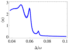
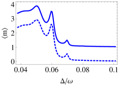
Figure 1: (a) The steady-state optical cavity mean photon number $\langle n\rangle\equiv\langle a^{\dagger}a\rangle$ as well as (b) the corresponding mechanical resonator mean phonon number $\langle m\rangle\equiv\langle b^{\dagger}b\rangle$ as a function of $\Delta/\omega$. Here $\chi=0.1$, $\epsilon/\omega=0.02$, $\kappa_{a}/\omega=2\cdot 10^{-3}$ and $\kappa_{b}/\omega=2\cdot 10^{-5}$, and only single-phonon processes were included. Also, $\bar{n}=1$ for solid lines, while $\bar{n}=0$ for short-dashed lines, respectively.

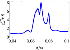
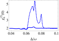
Figure 2: The steady-state second-order correlation function for (a) photons, $g^{(2)}_{a}(0)$, and (b) for phonons, $g^{(2)}_{b}(0)$, as a function of $\Delta/\omega$. The solid lines are for $\bar{n}=1$, while the short-dashed one for $\bar{n}=0$, respectively. Other parameters are as in Fig. 1.

III Numerical Results and Discussion

In Fig. 1 we present the numerical results of the steady-state mean photon and phonon numbers for a generic system with parameters within the considered regime with $\chi=0.1$, $\epsilon/\omega=0.02$, $\kappa_{a}/\omega=2\cdot 10^{-3}$ and $\kappa_{b}/\omega=2\cdot 10^{-5}$. These parameters are accessible experimentally. For instance, a similar set with $\omega\sim 1\rm{MHz}$, $g\sim 0.3\rm{MHz}$, $\kappa_{a}\sim 0.2\rm{MHz}$ and $\kappa_{b}\sim 150\rm{Hz}$ was reported in Ref. exp1 . For our case, also a good-cavity regime with $\omega\gg\kappa_{a}$ would be of interest, since a too strong photon loss washes out the predicted features. Furthermore, we considered here only one-phonon process, which corresponds to keeping terms up to $\chi^{2}$ in Eq. (6), respectively. Few interesting features can be observed: (i) In these parameter ranges, the steady-state phonon dynamics is quite sensitive on external temperature variations, (ii) the photon dynamics follows that of phonon one (see Appendix B), and vice versa, though with a different magnitude, and (iii) the peak frequency intervals equal the Kerr-like nonlinearity $\omega\chi^{2}$, see Hamiltonian (7). The latter result can be intuitively understood from the free-photon Hamiltonian plus the Kerr-like contribution, i.e. $\bar{H}_{0}=\hbar\bar{a}^{\dagger}\bar{a}(\Delta-\omega\chi^{2}\bar{a}^{\dagger}\bar{a})$, from where it follows that the effective detuning vanishes at $\Delta_{k}=k\omega\chi^{2}$ or $|\Delta_{k}-\Delta_{k\pm 1}|=\omega\chi^{2}\equiv g^{2}/\omega$. This reveals that the induced Kerr nonlinearity shifts the frequency of the corresponding photon Fock states, which can be detected by scanning the frequency of the cavity photons. Thus, the mean-phonon number dynamics can be extracted via detection of the mean-photon number’s quantum dynamics, while the coupling constant $g$ can be estimated if the mechanical motion frequency $\omega$ is known (or vice versa).

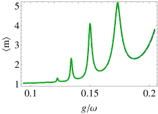
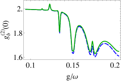
Figure 3: The steady-state behaviors of (a) the mean-phonon number $\langle m\rangle$ as well as (b) the second-order phonon-phonon correlation function $g^{(2)}_{b}(0)$ as a function of $\chi=g/\omega$. The dashed blue line is plotted for single-phonon whereas the green solid one for three-phonon processes, respectively. Here $\Delta/\omega=0.09$ and $\bar{n}=1$ while other parameters are as in Fig. (1).

Figure 2 shows the corresponding second-order correlation functions. The photon statistics changes from sub-Poissonian ($g^{(2)}_{a}(0)<1$) for $\Delta/\omega\lesssim 0.05$, to super-Poissonian ($g^{(2)}_{a}(0)\geq 2$) in the interval 0.06-0.08 and to quasi-coherent features ($g^{(2)}_{a}(0)\gtrapprox 1$ ) for $\Delta/\omega>0.08$. On the other hand, the phonon statistics exhibits quasi-thermal to super-Poissonian properties. Also in this case, the curves are characterized by a multi-peak structure. For smaller and negative $\Delta/\omega$, the lines in Figs. (1) and (2) remain flat. Notice that in the absence of vibrations, i.e. when $g=0$, the cavity mean-photon number and its correlation function are given by the following expressions in the steady-state:

$$\langle a^{\dagger}a\rangle = \epsilon^{2}/\bigl{(}\Delta^{2}+(\kappa_{a}/2)^{2}\bigr{)},~{}~{}{\rm and}$$

$$\langle a^{\dagger 2}a^{2}\rangle = \epsilon^{4}/\bigl{(}\Delta^{2}+(\kappa_{a}/2)^{2}\bigr{)}^{2},$$

leading to $g^{(2)}_{a}(0)\equiv\langle a^{\dagger 2}a^{2}\rangle/\langle a^{\dagger}a\rangle^{2}=1$. For an independent boson mode in thermal equilibrium with its surrounding thermal bath we obtain

$$\langle b^{\dagger}b\rangle=\bar{n},~{}~{}{\rm and}~{}~{}\langle b^{\dagger 2}b^{2}\rangle=2\bar{n}^{2},$$

with $g^{(2)}_{b}(0)\equiv\langle b^{\dagger 2}b^{2}\rangle/\langle b^{\dagger}b\rangle^{2}=2$.

In Fig. 3 we investigate the mean phonon number and its statistics as a function of $\chi=g/\omega$ for a fixed ratio $\Delta/\omega=0.09$. As can be seen in Fig. 1, for the particular coupling strength $g$ chosen ($\chi=0.1$) the mean-quanta numbers are quite small at this detuning. Figure 3 compares the case of single-phonon processes, i.e. keeping terms up to $\chi^{2}$ in Eq. (6), with the case of three-phonon processes, for which we consider all terms up to $\chi^{6}$ in Eq. (6). As a first observation, we notice that the mean-phonon number increases with the ratio $g/\omega$. The peaks are slightly higher for three-phonon processes, but the differences are barely noticeable in Fig. 3a. Furthermore, the maxima occur at $\chi_{k}$=$\sqrt{\Delta/(k\omega)}$, which for $\Delta/\omega=0.09$, give k=6, 5, 4 and 3. Also, the steady-state mean phonon number is direct proportional to the mean thermal phonon number $\bar{n}$ due to the environmental reservoir, see Appendix B. The second-order phonon-phonon correlation function changes accordingly and exhibits quasi-thermal features for $\bar{n}=1$. In this case, single-phonon and three-phonon processes become distinguished at higher ratios of $g/\omega$, see Fig. 3(b). Thus, multiphonon processes occur for higher ratios of $g/\omega$. It can be shown that also in this case the mean photon number dynamics is following the mean phonon number dynamics, albeit with a smaller scaling. Finally, we have also calculated higher-order phonon correlation functions multix ; multiy , i.e. $g^{(k)}_{b}(0)=\langle b^{\dagger k}b^{k}\rangle/\langle b^{\dagger}b\rangle^{k}$ as a function of $\Delta/\omega$ with $k\in\{3,4\}$. Our numerical results show that these curves closely follow the ones of $g^{(2)}_{b}(0)$, however with a larger magnitude. For instance, the peak at $\Delta/\omega=0.07$ appears for the third-order (fourth order) correlation function at the same position, but with a value of approx. 7.6 (39).

Our results confirm that the presence of a vibrating mirror changes significantly both the photon’s as well as the phonon quantum dynamics of an off-resonant pumped cavity optomechanical system. Moreover, the parameter range required to observe this behavior is within experimental reach exp1 ; exp2 ; exp3 and is close to those for photon blockade effect predicted in optomechanical systems phblk1 ; phblk2 . Finally, the analytical approaches proper to cavity optomecanics with a moving mirror equally apply to other related samples, like e.g., hybrid metal-dielectric cavities hdcav , plasmon-excitonic polaritons pep , superconducting qubits and quantum circuits qcirc or other types of nanomechanical resonators nmr , respectively, rendering our developed analytical approach relevant also for these systems.

IV Conclusions

We have investigated a cavity optomechanical setup where the detuning of the external coherent electromagnetic field frequency from the optical resonator’s one is different from the frequency (or its multiples) of one of the vibrating mirror. As a result, the quantum dynamics of this complex system is accompanied by multiple phonon absorption and emission processes. We have computed the mean-quanta numbers and the corresponding second-order correlation functions and described their properties. Particularly, we have found that the inter-peak frequency intervals observed in the quantum dynamics of the photon and phonon subsystem as a function of detuning equal the vibration-induced Kerr-like non-linearity. The photon mean-number dynamics follows that of the mean-phonon one which is convenient for monitoring the phonon quantum dynamics by photon detection. The corresponding second-order correlation functions also exhibit a multi-peak structure and are completely different from the fixed-mirror case. The photon-photon correlation function may exhibit sub-Poissonian to super-Poissonian photon statistics. The corresponding correlation function for phonons lies within quasi-thermal to thermal phonon statistics, characterized by super-Poissonian features. Furthermore, the second order phonon correlation function can be used to distinguish among the one- and few-phonon processes for stronger coupling strengths among the involved interacting subsystems. For a more detailed investigation of non-classical signatures, future work could focus on the Wigner function for representative parameter sets, or on so-called bundle correlation functions, $g^{(2)}_{2}(\tau)=\langle b^{\dagger 2}(0)b^{\dagger 2}(\tau)b^{2}(\tau)b^{2}(0)\rangle/\langle(b^{\dagger 2}b^{2})(0)\rangle\langle(b^{\dagger 2}b^{2})(\tau)\rangle$ multix ; multiy , which could reveal highly correlated phonon behaviour.

Appendix A Expanding the exponents up to $\chi^{4}$

In order to demonstrate the multi-phonon nature of the combined quantum dynamics, let us expand the exponents in the expression (13), i.e. $e^{\chi(\bar{b}-\bar{b}^{\dagger})}\bar{a}\bar{\rho}\bar{a}^{\dagger}e^{-\chi(\bar{b}-\bar{b}^{\dagger})}$, up to $\chi^{4}$ and keep the time-independent terms only, that is,

$$e^{\chi(\bar{b}-\bar{b}^{\dagger})}\bar{a}\bar{\rho}\bar{a}^{\dagger}e^{-\chi(\bar{b}-\bar{b}^{\dagger})}=\bar{a}\bar{\rho}\bar{a}^{\dagger}+\biggl{(}\bar{a}\bar{\rho}\bar{a}^{\dagger}\bigl{\{}\frac{\chi^{2}}{2!}(1-2\bar{b}\bar{b}^{\dagger})+\frac{\chi^{4}}{4!}(6\bar{b}^{2}\bar{b}^{\dagger 2}-12\bar{b}\bar{b}^{\dagger}+3)\bigr{\}}+H.c.\biggr{)}+\chi^{2}(1+\chi^{2})\biggl{(}\bar{b}\bar{a}\bar{\rho}\bar{a}^{\dagger}\bar{b}^{\dagger}$$

$$+\bar{b}^{\dagger}\bar{a}\bar{\rho}\bar{a}^{\dagger}\bar{b}\biggr{)}-\frac{\chi^{4}}{2}\biggl{(}\bar{b}\bar{a}\bar{\rho}\bar{a}^{\dagger}\bar{b}\bar{b}^{\dagger 2}+\bar{b}^{\dagger}\bar{a}\bar{\rho}\bar{a}^{\dagger}\bar{b}^{2}\bar{b}^{\dagger}+H.c.\biggr{)}+\frac{\chi^{4}}{4}\biggl{(}\bar{b}^{2}\bar{a}\bar{\rho}\bar{a}^{\dagger}\bar{b}^{\dagger 2}+(1-2\bar{b}\bar{b}^{\dagger})\bar{a}\bar{\rho}\bar{a}^{\dagger}(1-2\bar{b}\bar{b}^{\dagger})+\bar{b}^{\dagger 2}\bar{a}\bar{\rho}\bar{a}^{\dagger}\bar{b}^{2}\biggr{)}.$$

(20)

When considering the photon-phonon distribution function $P_{n_{1}n_{2},mm}$, then from (20) one can observe that terms proportional at least to $\chi^{2}$ contribute to single-phonon processes, whereas those proportional to $\chi^{4}$ - to two-phonon processes, respectively. For instance, the last term from the first line of expression (20) accounts for single-phonon processes where the phonon number changes by $\pm 1$, i.e. $m\pm 1$. On the other side, the last term from (20) describes two-phonon processes where the phonon number modifies by $\pm 2$, $m\pm 2$. Thus, the expression (20), expanded up to $\chi^{4}$ terms, describes simultaneously single- and two-phonon processes, respectively. Also, single-phonon processes are influenced by the second-order ones, i.e. there is a contribution to single-phonon processes coming from $\chi^{4}$ terms.

Generalizing now, one can state that $N$-phonon processes are described by terms proportional to $\chi^{2N}$. There is a contribution to $N$-phonon processes which arises from higher order terms proportional to $\chi^{2(N+1)}$. This way, depending on a certain power of $\chi$, one can investigate the multiphonon quantum dynamics of the cavity optomechanical system.

Appendix B Relationship among the optical and phonon modes

In what follows, we shall give details on how the mean cavity photon and mean phonon numbers are interconnected in the dispersive interaction regime investigated here. The master equation (6), containing terms up to $\chi^{2}$ for simplicity and in the considered approximations, reads

$$\frac{d}{dt}\bar{\rho}(t) + \frac{i}{\hbar}[\bar{H},\bar{\rho}]=$$

$$- \frac{\kappa_{a}}{2}\biggl{(}\bar{a}^{\dagger}\bar{a}\bar{\rho}-e^{\chi(\bar{b}-\bar{b}^{\dagger})}\bar{a}\bar{\rho}\bar{a}^{\dagger}e^{-\chi(\bar{b}-\bar{b}^{\dagger})}\biggr{)}$$

$$- \frac{\kappa_{b}}{2}(1+\bar{n})\biggl{(}[\bar{b}^{\dagger},\bar{b}\bar{\rho}]+\chi^{2}[\bar{a}^{\dagger}\bar{a},\bar{a}^{\dagger}\bar{a}\bar{\rho}]\biggr{)}$$

$$- \frac{\kappa_{b}}{2}\bar{n}\biggl{(}[\bar{b},\bar{b}^{\dagger}\bar{\rho}]+\chi^{2}[\bar{a}^{\dagger}\bar{a},\bar{a}^{\dagger}\bar{a}\bar{\rho}]\biggr{)}+H.c.,$$

where

$$\bar{H} = \hbar\Delta\bar{a}^{\dagger}\bar{a}+\hbar\omega\bar{b}^{\dagger}\bar{b}+\hbar\epsilon(\bar{a}+\bar{a}^{\dagger})\bigl{\{}1-\chi^{2}(\bar{b}^{\dagger}\bar{b}+\bar{b}\bar{b}^{\dagger})/2\bigr{\}}$$ (22)

$$- \omega\chi^{2}(\bar{a}^{\dagger}\bar{a})^{2}.$$

The exponent term from the first line of the damping part of the above master equation can be obtained from (20) while setting $\chi^{4}\to 0$. Then, in the steady-state, from the master equation (LABEL:app2) one can easily show that

$$\langle\bar{b}^{\dagger}\bar{b}\rangle=\bar{n}+\chi^{2}\frac{\kappa_{a}}{\kappa_{b}}\langle\bar{a}^{\dagger}\bar{a}\rangle,$$ (23)

while from Eqs. (4), one finally arrives at the relationship among the steady-state mean phonon and photon numbers, namely,

$$\langle b^{\dagger}b\rangle = \langle\bar{b}^{\dagger}\bar{b}\rangle+\chi^{2}\langle\bar{a}^{\dagger 2}\bar{a}^{2}\rangle$$ (24)

$$= \bar{n}+\chi^{2}\frac{\kappa_{a}}{\kappa_{b}}\langle\bar{a}^{\dagger}\bar{a}\rangle+\chi^{2}\langle\bar{a}^{\dagger 2}\bar{a}^{2}\rangle.$$

One can observe here that there is an almost linear dependence between mean phonon and cavity photon numbers, respectively, since the last term may give little contribution as long as $\chi\ll 1$. In addition, we have assumed that $\kappa_{a}/\kappa_{b}\gg 1$ . Thus, detecting the cavity photons one can estimate the mean phonon number and vice versa.

References

- (1) D. F. Walls, and G. J. Milburn, Quantum Optics (Springer, Berlin, Heidelberg, 2008).
- (2) M. Aspelmeyer, T. J. Kippenberg, and F. Marquardt, Cavity optomechanics, Rev. Mod. Phys. 86, 1391 (2014).
- (3) C. L. Degen, F. Reinhard, and P. Cappellaro, Quantum sensing, Rev. Mod. Phys. 89, 035002 (2017).
- (4) V. B. Braginskii, Classical and quantum restrictions on the detection of weak disturbances of a macroscopic oscillator, Sov. Phys. JETP 26, 831 (1968).
- (5) I. Pikovski, M. R. Vanner, M. Aspelmeyer, M. S. Kim, and C. Brukner, Probing Planck-scale physics with quantum optics, Nature Physics 8, 393 (2012).
- (6) G. A. Brawley, M. R. Vanner, P. E. Larsen, S. Schmid, A. Boisen, and W.P. Bowen, Nonlinear optomechanical measurement of mechanical motion, Nature Communications 7:10988, 1 (2016).
- (7) S. Qvarfort, A. Serafini, P. F. Barker, and S. Bose, Gravimetry through non-linear optomechanics, Nature Communications 9:3690, 1 (2018).
- (8) S. Gigan, R. Böhm, M. Paternostro, F. Blaser, G. Langer, J. B. Hertzberg, K. C. Schwab, D. Bäuerle, M. Aspelmeyer, and A. Zeilinger, Self-cooling of a micromirror by radiation pressure, Nature (London) 444, 67 (2006).
- (9) O. Arcizet, P. F. Cohadon, T. Briant, M. Pinard, and A. Heidmann, Radiation-pressure cooling and optomechanical instability of a micromirror, Nature (London) 444, 71 (2006).
- (10) I. Wilson-Rae, N. Nooshi, W. Zwerger, and T. J. Kippenberg, Theory of Ground State Cooling of a Mechanical Oscillator Using Dynamical Backaction, Phys. Rev. Lett. 99, 093901 (2007).
- (11) F. Marquardt, J. P. Chen, A. A. Clerk, and S. M. Girvin, Quantum Theory of Cavity-Assisted Sideband Cooling of Mechanical Motion, Phys. Rev. Lett. 99, 093902 (2007).
- (12) J. D. Teufel, T. Donner, D. Li, J. W. Harlow, M. S. Allman, K. Cicak, A. J. Sirois, J. D. Whittaker, K. W. Lehnert, and R. W. Simmonds, Sideband cooling of micromechanical motion to the quantum ground state, Nature (London) 475, 359 (2011).
- (13) J. Chan, T. P. Mayer Alegre, A. H. Safavi-Naeini, J. T. Hill, A. Krause, S. Gröblacher, M. Aspelmeyer, and O. Painter, Laser cooling of a nanomechanical oscillator into its quantum ground state, Nature (London) 478, 89 (2011).
- (14) S. Mancini, V. I. Man’ko, and P. Tombesi, Ponderomotive control of quantum macroscopic coherence, Phys. Rev. A 55, 3042 (1997).
- (15) S. Bose, K. Jacobs, and P. L. Knight, Preparation of nonclassical states in cavities with a moving mirror, Phys. Rev. A 56, 4175 (1997).
- (16) G. S. Agarwal, and S. Huang, Electromagnetically induced transparency in mechanical effects of light, Phys. Rev. A 81, 041803(R) (2010).
- (17) S. Weis, R. Riviere, S. Deleglise, E. Gavartin, O. Arcizet, A. Schliesser, and T. J. Kippenberg, Optomechanically Induced Transparency, Science 330, 1520 (2010).
- (18) H. Xionga, and Y. Wu, Fundamentals and applications of optomechanically induced transparency, Applied Phys. Rev. 5, 031305 (2018).
- (19) G. S. Agarwal, and S. Huang, Optomechanical systems as single-photon routers, Phys. Rev. A 85, 021801(R) (2012).
- (20) W.-T. Liao, and A. Pálffy, Optomechanically induced transparency of x-rays via optical control, Scientific Reports 7: 321, 1 (2017).
- (21) S. Aldana, Ch. Bruder, and A. Nunnenkamp, Equivalence between an optomechanical system and a Kerr medium, Phys. Rev. A 88, 043826 (2013).
- (22) P. D. Drummond, and D. F. Walls, Quantum theory of optical bistability. I. Nonlinear polarisability model, J. Phys. A 13, 725 (1980).
- (23) F. Marquardt, J. G. E. Harris, and S. M. Girvin, Dynamical Multistability Induced by Radiation Pressure in High-Finesse Micromechanical Optical Cavities, Phys. Rev. Lett. 96, 103901 (2006).
- (24) M. A. Macovei, Measuring photon-photon interactions via photon detection, Phys. Rev. A 82, 063815 (2010).
- (25) A. Miranowicz, M. Paprzycka, Y.-x. Liu, J. Bajer, and F. Nori, Two-photon and three-photon blockades in driven nonlinear systems, Phys. Rev. A 87, 023809 (2013).
- (26) D. Vitali, S. Gigan, A. Ferreira, H. R. Böhm, P. Tombesi, A. Guerreiro, V. Vedral, A. Zeilinger, and M. Aspelmeyer, Optomechanical Entanglement between a Movable Mirror and a Cavity Field, Phys. Rev. Lett. 98, 030405 (2007).
- (27) L. Tian, Robust Photon Entanglement via Quantum Interference in Optomechanical Interfaces, Phys. Rev. Lett. 110, 233602 (2013).
- (28) Z. R. Gong, H. Ian, Y.-x. Liu, C. P. Sun, and F. Nori, Effective Hamiltonian approach to the Kerr nonlinearity in an optomechanical system, Phys. Rev. A 80, 065801 (2009).
- (29) P. Rabl, Photon Blockade Effect in Optomechanical Systems, Phys. Rev. Lett. 107, 063601 (2011).
- (30) F. Zou, L.-B. Fan, J.-F. Huang, and J.-Q. Liao, Enhancement of few-photon optomechanical effects with cross-Kerr nonlinearity, Phys. Rev. A 99, 043837 (2019).
- (31) K. Stannigel, P. Rabl, A. S. Sorensen, P. Zoller, and M. D. Lukin, Optomechanical Transducers for Long-Distance Quantum Communication, Phys. Rev. Lett. 105, 220501 (2010).
- (32) D. E. Chang, V. Vuletic, and M. D. Lukin, Quantum nonlinear optics — photon by photon, Nature Photonics 8, 685 (2014).
- (33) M. A. Nielsen, and I. L. Chuang, Quantum Computation and Quantum Information (Cambridge University Press, Cambridge, 2000).
- (34) A. Nunnenkamp, K. Borkje, and S. M. Girvin, Single-Photon Optomechanics, Phys. Rev. Lett. 107, 063602 (2011).
- (35) A. Kronwald, M. Ludwig, and F. Marquardt, Full photon statistics of a light beam transmitted through an optomechanical system, Phys. Rev. A 87, 013847 (2013).
- (36) S. Gröblacher, K. Hammerer, M. R. Vanner, and M. Aspelmeyer, Observation of strong coupling between a micromechanical resonator and an optical cavity field, Nature 460, 724 (2009).
- (37) R. Leijssen, and E. Verhagen, Strong optomechanical interactions in a sliced photonic crystal nanobeam, Scientific Reports 5:15974, 1 (2015).
- (38) G. A. Peterson, S. Kotler, F. Lecocq, K. Cicak, X. Y. Jin, R.W. Simmonds, J. Aumentado, and J. D. Teufel, Ultrastrong Parametric Coupling between a Superconducting Cavity and a Mechanical Resonator, Phys. Rev. Lett. 123, 247701 (2019).
- (39) M. Kiffner, M. Macovei, J. Evers, and C. H. Keitel, Vacuum-induced processes in multilevel atoms, Progress in Optics 55, 85 (2010).
- (40) J. Qian, A. A. Clerk, K. Hammerer, and F. Marquardt, Quantum Signatures of the Optomechanical Instability, Phys. Rev. Lett. 109, 253601 (2012).
- (41) R. J. Glauber, The Quantum Theory of Optical Coherence, Phys. Rev. 130, 2529 (1963).
- (42) J. D. Cohen, S. M. Meenehan, G. S. MacCabe, S. Gröblacher, A. H. Safavi-Naeini, F. Marsili, M. D. Shaw, and O. Painter, Phonon counting and intensity interferometry of a nanomechanical resonator, Nature 520, 522 (2015).
- (43) C. Sánchez Munoz, E. del Valle, A. González Tudela, K. Müller, S. Lichtmannecker, M. Kaniber, C. Tejedor, J. J. Finley, and F. P. Laussy, Emitters of N-photon bundles, Nat. Photonics 8, 550 (2014).
- (44) Q. Bin, X.-Y. Lü, F. P. Laussy, F. Nori, and Y. Wu, N-Phonon Bundle Emission via the Stokes Process, Phys. Rev. Lett. 124, 053601 (2020).
- (45) M. K. Dezfouli, R. Gordon, and S. Hughes, Molecular Optomechanics in the Anharmonic Cavity-QED Regime Using Hybrid Metal-Dielectric Cavity Modes, ACS Photonics 6, 1400 (2019).
- (46) T. Neuman, J. Aizpurua, and R. Esteban, Quantum theory of surface-enhanced resonant Raman scattering (SERRS) of molecules in strongly coupled plasmon-exciton systems, Nanophotonics 9(2), 295 (2020).
- (47) S. N. Shevchenko, and A. N. Omelyanchouk, Multiphoton transitions in Josephson-junction qubits, Low Temperature Physics 38, 283 (2012).
- (48) Y. Greenberg, Y. Pashkin, and E. Il’ichev, Nanomechanical resonators, Physics-Uspekhi, 182, 407 (2012).