Exact time dependence of the cumulants of a tracer position in a dense lattice gas

Abstract

We develop a general method to calculate the exact time dependence of the cumulants of the position of a tracer particle in a dense lattice gas of hardcore particles. More precisely, we calculate the cumulant generating function associated with the position of a tagged particle at arbitrary time, and at leading order in the density of vacancies on the lattice. In particular, our approach gives access to the short-time dynamics of the cumulants of the tracer position – a regime in which few results are known. The generality of our approach is demonstrated by showing that it goes beyond the case of a symmetric 1D random walk, and covers the important situations of (i) a biased tracer; (ii) comb-like structures; and (iii) $d$-dimensional situations.

Introduction.— Understanding and characterising tracer diffusion in crowded environments is central in numerous biological and physical contexts. In living systems, the interplay between the diffusion of tracer particles (fuelled by thermal fluctuations, active processes, or chemical reactions) and complex environments (which generally hinder their motion) controls many biological processes Höfling and Franosch (2013). Quantifying tracer diffusion can also be used as a mean to probe the mechanical and rheological properties of different systems, such as colloidal suspensions or complex fluids, through passive and active microrheology Wilson and Poon (2011); Squires and Mason (2010); Puertas and Voigtmann (2014).

These examples, in which the statistical properties of tracer particles are controlled by the interactions with their environment, are the motivation for a whole field of theoretical research. Among the different routes that were employed to characterise the statistics of diffusing particles in crowded environments, lattice gases of hardcore particles that jump at exponentially distributed times (often referred to as exclusion processes) have been the subject of many studies, and have become central models of statistical mechanics Mallick (2011); Chou et al. (2011). In particular, such models were widely employed to compute the diffusion coefficient of a tracer particle. In dimension 2 or greater, different mean-field-like approximations were designed to estimate the diffusion coefficient of the tracer as the function of the density of the bath Nakazato and Kitahara (1980); Tahir-Kheli and Elliott (1983); van Beijeren and Kutner (1985). In the case of one-dimensional systems, one can mention recent achievements which resulted in the derivation of exact results concerning tracer properties, including the calculation of its large deviations Imamura et al. (2017); Krapivsky et al. (2015, 2014); Hegde et al. (2014), and of bath-tracers correlations Poncet et al. (2021); Grabsch et al. (2021).

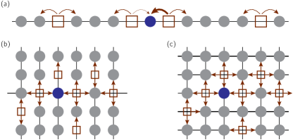
Figure 1: For each of the considered geometries (1D (a), comb (b), 2D (c)), the continuous-time random walks of the particles are mirrored by the random walks of the vacancies (brown squares). The latter perform continuous-time nearest-neighbor symmetric random walks.

However, these results, whether exact or approximate, are generally valid only in the long-time limit, because their derivation relies on hydrodynamic limits or large deviations approaches Imamura et al. (2017); Krapivsky et al. (2015, 2014); Hegde et al. (2014); Poncet et al. (2021); Grabsch et al. (2021). A notable exception is provided in the dense limit by the approach by Brummelhuis and Hilhorst  Brummelhuis and Hilhorst (1989, 1988), later extended to the case of a biased tracer Bénichou and Oshanin (2002); Illien et al. (2013); Bénichou et al. (2013); Illien et al. (2014). However, we stress that this approach is intrinsically discrete in time. Even though the real continuous-time description of exclusion processes, where particles jump at exponential times as defined above, is retrieved in the long-time limit, this approach fails to predict the dynamics of the tracer at short and intermediate times. So far, the only available results at arbitrary time concern the first cumulants in the low-density regime with immobile bath particles Leitmann and Franosch (2017, 2013), the high-density regime for a symmetric tracer in 1D Poncet et al. (2021), or the 1D situation at arbitrary density, but under a formulation that does not allow the derivation of fully explicit results Imamura et al. (2021). Finally, a general quantitative description of the dynamics of the tracer for arbitrary time is lacking.

In this Letter, we fill this gap and calculate the exact and complete time dependence of the cumulants of a tracer particle in a dense lattice gas. We develop a general methodology which covers the important cases of (i) a biased tracer; (ii) comb-like structures; and (iii) $d$-dimensional situations. These results fully quantify the dynamics of tracer particles in exclusion processes, which are paradigmatic models of statistical mechanics.

Model and outline of the calculations.— We consider a lattice populated by particles at a density $\rho$ between 0 and 1, which are initially positioned uniformly at random on the lattice, with the restriction that there can only be one particle per site. We adopt the usual dynamics of exclusion processes, which evolve in continuous-time, and we assume that each particle has an exponential clock of time constant $\tau=1$. When the clocks ticks, each particle chooses to jump on one of its $z$ neighboring sites with probability $1/z$. If the arrival site is empty, the jump is done. Otherwise, if the arrival site is occupied, the jump is canceled. Note that, in 1D, this process corresponds to the celebrated Symmetric Exclusion Process or SEP Mallick (2011); Chou et al. (2011).

The tagged particle (TP) is initially at the origin $\boldsymbol{x}(0)=0$ and we study its displacement with time $\boldsymbol{x}(t)=(x_{1}(t),\dots,x_{d}(t))$. We define the cumulant-generating function (CGF) $\psi(\boldsymbol{k},t)\equiv\ln\langle e^{i\boldsymbol{k}\cdot\boldsymbol{x}(t)}\rangle$. We will consider the cumulants of the position projected onto one direction of the lattice, say direction 1 ($x_{1}(t)=\boldsymbol{x}(t)\cdot\boldsymbol{e}_{1}$):

$$\kappa_{n}(t)=\frac{1}{\mathrm{i}^{n}}\left(\frac{\partial^{n}\psi(\boldsymbol{k},t)}{\partial{k_{1}}^{n}}\right)_{\boldsymbol{k}=\mathbf{0}}.$$ (1)

Our goal here is the determination of the cumulant-generating function $\psi(\boldsymbol{k},t)$ and the cumulants $\kappa_{n}(t)$ in the high-density limit $\rho\to 1$, and for arbitrary time $t$. We will define their rescaled high-density limit as $\bar{\kappa}_{n}=\lim_{\rho\to 1}\kappa_{n}/(1-\rho)$, where $\rho_{0}=1-\rho$ is the density of vacancies on the lattice.

From a single vacancy to the dense regime.— Relying on the derivation that was originally proposed in a discrete-time description Brummelhuis and Hilhorst (1988, 1989), we start by considering a system of finite size $N$ in which all the sites are occupied except $M$ of them (Fig. 1). We call these empty sites vacancies, and their fraction is denoted by $\rho_{0}=M/N=1-\rho$. Now, in the high-density limit ($\rho_{0}=M/N\to 0$), we note that the vacancies perform independent random walks and interact independently with the TP. We neglect events of order $\mathcal{O}(\rho_{0}^{2})$ in which two vacancies interact with each other, compared to events of order $\mathcal{O}(\rho_{0})$ in which one vacancy interacts with the TP. This gives exact results at linear order in the density of vacancies $\rho_{0}$. We call $p_{1}(\boldsymbol{x}|\boldsymbol{y},t)$ the probability that, in a system with a single vacancy initially at $\boldsymbol{y}$, the TP has reached site $\boldsymbol{x}$ at time $t$ knowing that it started from the origin. In Fourier space, the probability to find the tracer at a given location given that the vacancies were initially at positions $\boldsymbol{y}_{1},\dots,\boldsymbol{y}_{M}$ can be written as a product of single-vacancy propagators $p_{1}$ (see Section I in Supplemental Material (SM) SM ). Averaging over the initial positions of the vacancies and taking the thermodynamic limit of $M,N\to\infty$ with fixed $\rho_{0}$, the cumulant-generating function reads

$$\lim_{\rho_{0}\to 0}\frac{\psi(\boldsymbol{k},t)}{\rho_{0}}=\sum_{\boldsymbol{y}\neq 0}\left(\tilde{p}_{1}(\boldsymbol{k}|\boldsymbol{y},t)-1\right),$$ (2)

where we use the following convention for Fourier transforms $\tilde{f}(\boldsymbol{k})=\sum_{\boldsymbol{x}}\mathrm{e}^{\mathrm{i}\boldsymbol{k}\cdot\boldsymbol{x}}f(\boldsymbol{x})$. Let us emphasize the meaning of Eq. (2): the full probability law of a TP at high density is encoded in a much simpler quantity, namely the propagator of the tracer in a system where there is only one vacancy. This expression is the continuous-time counterpart of the discrete-time approach Brummelhuis and Hilhorst (1988, 1989).

Using standard techniques from the theory of random walks on lattices Hughes (1995), the single-vacancy propagators $p_{1}(\boldsymbol{x}|\boldsymbol{y},t)$ can be expressed in terms of first-passage time densities associated with the random walk performed by a vacancy on the considered lattice, namely $f(\mathbf{0}|\boldsymbol{y},t)$, the probability for the vacancy to reach the origin for the first time at time $t$ knowing that it started from site $\boldsymbol{y}$, and $f^{*}(\mathbf{0}|\boldsymbol{e}_{\mu}|\boldsymbol{y},t)$, the same quantity but conditioned on the fact that the vacancy was at site $\boldsymbol{e}_{\mu}$ before its last jump. The relation between these quantities is obtained by counting the interactions between the vacancy and the tracer up to time $t$.

For clarity we consider separately: (i) the situation where the lattice is tree-like, i.e. the situation where there is a single minimum-length path linking two arbitrary sites of the lattice (this will cover the case of one-dimensional and comb-like lattices); (ii) the situation where the lattice is looped, i.e. the situation where there is more than one minimum-length path linking two arbitrary sites of the lattice (this will cover the case of lattices of dimension 2 and higher).

Tree-like lattices.— We first consider tree-like lattices as shown in Figs. 1(a) and 1(b). We show in SM (Section II of SM ) that, on these geometries, the single-vacancy propagator is simply related to the FPT densities through the relation

$$\hat{\tilde{p}}_{1}(k|\boldsymbol{y},u)=\frac{1}{u}\left[1+\left(e^{i\mu k}-1\right)\frac{1-\hat{f}_{-\mu}(u)}{1-\hat{f}_{1}(u)\hat{f}_{-1}(u)}\hat{f}(\mathbf{0}|\boldsymbol{y},u)\right],$$ (3)

where we introduce the shorthand notation $\hat{f}_{\nu}(u)=\hat{f}(\mathbf{0}|\boldsymbol{e}_{\nu},u)$. One can use this expression into Eq. (2) to obtain the cumulant-generating function at high density in terms of first-passage quantities of a single vacancy. The last step consists in studying the random walk of a single vacancy to compute $\hat{f}(\mathbf{0}|\boldsymbol{y},u)$.

We first apply this formalism to the case of a 1D lattice (Fig. 1(a)). We consider the general situation of a biased tracer which jumps with probability $p_{+}$ to the right and $p_{-}$ to the left. A vacancy then performs a nearest-neighbor random walk, which is symmetric far away from the tracer and perturbed in its vicinity. Considering a vacancy starting from site $y$ and partitioning over the instant of first visit to site $\mu=\mathrm{sgn}(y)$, it is straightforward to show that $\hat{f}_{y}(u)=\hat{f}^{\mathrm{UB}}_{|y|-1}(u)\hat{f}_{\mu}(u)$ SM , where we introduced the following notation for the Laplace transform: $\hat{\varphi}(u)=\int_{0}^{\infty}\mathrm{e}^{-ut}\varphi(t)\mathrm{d}t$, the shorthand notation $f_{y}(t)=f(0|y,t)$, and where the superscript UB denotes the FPT density of the vacancy to the origin when the tracer is unbiased. We finally get (Section III in SM ):

$$\hat{f}_{y}(u)=\frac{1+\mu s}{1+\mu s\alpha}\alpha^{|y|},$$ (4)

where $\alpha=1+u-\sqrt{u(2+u)}$ and where $s=p_{+}-p_{-}$ is the bias. Inserting the first-passage quantities computed in Eq. (4) into the expression of the propagator with a single vacancy [Eq. (3)], and then back into the expression of the cumulant-generating function [Eq. (2)], we obtain, after Laplace inversion:

$$\lim_{\rho_{0}\to 0}\frac{\psi(k,t)}{\rho_{0}}=te^{-t}[\text{I}_{0}(t)+\text{I}_{1}(t)](\cos k-1+is\sin k),$$ (5)

where $\text{I}_{0}$ and $\text{I}_{1}$ are modified Bessel functions of the first kind Abramowitz and Stegun (1965). In the unbiased case $s=0$, we retrieve previous results for a symmetric tracer in the SEP Poncet et al. (2021). The first implication is that we have the full time-dependence of the even and odd cumulants,

$${\bar{\kappa}_{2n}(t)} = te^{-t}[\text{I}_{0}(t)+\text{I}_{1}(t)],$$ (6)

$${\bar{\kappa}_{2n+1}(t)} = ste^{-t}[\text{I}_{0}(t)+\text{I}_{1}(t)].$$ (7)

At short time, we find that the cumulants obey $\bar{\kappa}_{2n}(t)\sim t$ and $\bar{\kappa}_{2n+1}(t)\sim st$. This means in particular that the fluctuations of the tracer are diffusive, and that the displacement of a biased TP $\kappa_{1}$ is ballistic. At large time, we retrieve the known expressions Arratia (1983); Illien et al. (2013); Imamura et al. (2017): $\bar{\kappa}_{2n}(t)\sim\sqrt{{2t/\pi}}$ and $\bar{\kappa}_{2n+1}(t)\sim s\sqrt{{2t/\pi}}$. At all times, the results from Eqs. (6) and (7) are in perfect agreement with numerical simulations and shown on Fig. 2.

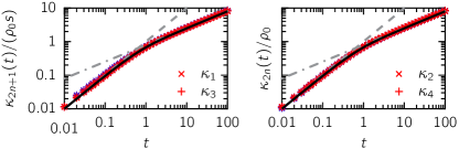
Figure 2: Time dependence of the odd (left) and even (right) cumulants of a TP in 1D ($\rho_{0}=0.02$) for different values of the bias (from blue to red: $s=0$, $0.2$, $0.5$, $0.8$, $1$). Symbols are the results from numerical simulations (see Section IX of SM for details). The black lines are the predictions from Eqs. (6) and (7), the gray lines are the asymptotic regimes at short and large times.

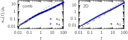
Figure 3: Cumulants of the position of a tracer constrained to move on the backbone of a comb lattice (left) and on a 2D lattice (right). Vacancy density $\rho_{0}=0.01$. The symbols correspond to the results from numerical simulations, the solid line is obtained from the inversion of the expression in Laplace domain [Eq. (9) and (15)] using the Stehfest algorithm. The short-time (dashed line) and long-time (dash-dotted line) asymptotics are given in the text.

We further illustrate the generality of our method by considering the important case of a comb lattice, a lattice made of a line, called the backbone, on which other lines, called the teeth, are connected (Fig. 1(b)). This structure has been widely used to describe diffusion on percolation clusters Ben-avraham and Havlin (2005). From now on and for simplicity, we restrict ourselves to the case of a symmetric tracer constrained to move on the backbone of the lattice. Relying on the same methodology as before, the density of first-passage time to the origin of a vacancy starting from site $(y_{1},y_{2})$ reads (Section IV of SM )

$$\hat{f}(0,0|y_{1},y_{2};u)=\begin{cases}\hat{f}_{1}(\hat{f}_{\parallel})^{|y_{1}|-1}\hat{f}_{\perp}\alpha^{|y_{2}|-1}&\text{if $y_{2}\neq 0$},\\ \hat{f}_{1}(\hat{f}_{\parallel})^{|y_{1}|-1}&\text{if $y_{2}=0$}.\end{cases}$$ (8)

where we introduced the shorthand notations $\hat{f}_{\mu}=\hat{f}(0,0|\mu,0,u)$, $\hat{f}_{\parallel}=\hat{f}(1,0|2,0,u)$ and $\hat{f}_{\perp}=\hat{f}(1,0|1,1,u)$, which can all be easily expressed in terms of $\alpha$ (Section IV in SM ). Introducing Eq. (8) into Eq. (3), we finally obtain

$$\lim_{\rho_{0}\to 0}\frac{\psi(k,u)}{\rho_{0}}=\hat{K}(u)(\cos k-1),$$ (9)

$$\text{with~{}}\hat{K}(u)=(2-\alpha)(\alpha^{2}-\alpha+2)/\{u(\alpha-1)$$

$$\times[u(2-\alpha)+\beta-4\alpha+6][u(\alpha-2)+\beta+2\alpha-2]\},$$

where $\beta=\sqrt{[(2+u)\alpha-2u-2][(3+u)\alpha-2u-4]}$. While odd cumulants are null (for symmetry reasons, and as can be seen from Eq. (9)), all the even cumulants are equal, and given by $\hat{\bar{\kappa}}_{\text{even}}(u)=\hat{K}(u)$. We deduce, after Laplace inversion, the short-time and long-time expansions: $K(t)\underset{t\to 0}{\sim}t$ and $K(t)\underset{t\to\infty}{\sim}\frac{2^{3/4}}{3\Gamma(3/4)}t^{3/4}$. Note that the long-time limit in the case of a symmetric tracer corresponds to the result we derived in discrete time Bénichou et al. (2015). For arbitrary time, we invert the cumulants numerically using the Stehfest algorithm. Numerical simulations are in perfect agreement with our analytical results (Fig. 3). Note that it is known that the two limits $t\to\infty$ and $\rho_{0}\to 0$ do not commute, which mirrors the existence of a subtle ultimate diffusive regime Bénichou et al. (2015), that we do not intend to describe here.

Looped lattices.— We finally consider the key situation of $d$-dimensional lattices. Note that the geometry can be general, each of the spatial directions of the lattice being either be infinite or finite with periodic boundary conditions, in such a way that the lattice remains translation-invariant. The CGF of the position of a symmetric tracer now reads (Section V in SM )

$$\lim_{\rho_{0}\to 0}\frac{\hat{\psi}(\boldsymbol{k},u)}{\rho_{0}}=-\sum_{j=1}^{d}\hat{\Delta}(\boldsymbol{k}|\boldsymbol{e}_{j},u)\hat{f}^{\prime}_{j}(u),$$ (10)

where we defined $f^{\prime}_{\nu}(t)=\sum_{\boldsymbol{y}\neq\mathbf{0}}f^{*}(\mathbf{0}|\boldsymbol{e}_{\nu}|\boldsymbol{y};t)$ and

$$\hat{\Delta}(\boldsymbol{k}|\boldsymbol{e}_{j},u)=\frac{2(1-\cos q_{j})}{u}-\frac{1}{u}\sum_{\mu,\nu}\left[1-\mathrm{e}^{-\mathrm{i}\boldsymbol{k}\cdot\boldsymbol{e}_{\nu}}\right]$$

$$\times\left\{[{\bf I}-{\bf T}]^{-1}\right\}_{\nu,\mu}\mathrm{e}^{\mathrm{i}{\boldsymbol{k}}\cdot\boldsymbol{e}_{\mu}}\sum_{\epsilon=\pm 1}\mathrm{e}^{-\epsilon\mathrm{i}q_{j}}\hat{f}^{*}(\mathbf{0}|\boldsymbol{e}_{\mu}|\epsilon\boldsymbol{e}_{j},u),$$ (11)

where $\mathbf{I}$ is the identity of size $2d$ and the matrix ${\rm{\bf T}}$ has the entries ${\rm{\bf T}}_{\mu,\nu}=\mathrm{e}^{\mathrm{i}\boldsymbol{k}\cdot{\bf e_{\nu}}}\hat{f}^{*}({\bf 0}|\boldsymbol{e}_{\nu}|-\boldsymbol{e}_{\mu};u)$ .

The final step of the calculation consists in determining the conditional FPT $f^{*}$ in terms of well-known quantities, namely the propagators associated to a discrete-time random walk on a lattice. The starting point of this calculation is the following relation, which consists in partitioning the random walk performed by the vacancy over the time of first visits to the origin:

$$\int_{0}^{t}\mathrm{d}t_{0}\frac{\chi(t_{0})}{2d}p(\boldsymbol{e}_{\mu}|\boldsymbol{y},t-t_{0})=\int_{0}^{t}\mathrm{d}t_{0}f^{*}(\mathbf{0}|\boldsymbol{e}_{\mu}|\boldsymbol{y},t_{0})\Psi(t-t_{0})$$

$$+\int_{0}^{t}\mathrm{d}t_{0}\int_{0}^{t-t_{0}}\mathrm{d}t_{1}\;\frac{1}{2d}\chi(t-t_{0}-t_{1})f(\mathbf{0}|\boldsymbol{y},t_{0})p(\boldsymbol{e}_{\mu}|\mathbf{0},t_{1}),$$ (12)

where $\Psi(t)=1-\int_{0}^{t}\mathrm{d}t^{\prime}\;\chi(t^{\prime})$ is the probability that the walker did not move during a time $t$. It is then straighforward to express the conditional FPTs $f^{*}$ in terms of the continuous-time occupation probabilities $p(\boldsymbol{r}|\boldsymbol{r}_{0},t)$ (probability to find a vacancy at site $\boldsymbol{r}$ at time $t$ knowing that it started from site $\boldsymbol{r}_{0}$). Finally, relying on the relation between the propagators $p$ and their discrete-time counterpart $P_{\boldsymbol{r}}^{(n)}$ (probability to find the walker at site $\boldsymbol{r}$ after $n$ steps knowing that it started from the origin) Hughes (1995), we get the relations (Section VI in SM )

$$\hat{f}^{*}(\mathbf{0}|\boldsymbol{e}_{\mu}|\boldsymbol{y},u) = \frac{\hat{\chi}}{2d}\left[\hat{P}_{\boldsymbol{e}_{\mu}-\boldsymbol{y}}(\hat{\chi})-\frac{\hat{P}_{\boldsymbol{y}}(\hat{\chi})\hat{P}_{\boldsymbol{e}_{\mu}}(\hat{\chi})}{\hat{P}_{\mathbf{0}}(\hat{\chi}(u))}\right],$$ (13)

$$\hat{f}^{\prime}_{\mu}(u) = \frac{1}{2d}\frac{\hat{\chi}}{1-\hat{\chi}}\left[1-\frac{\hat{P}_{\boldsymbol{e}_{\mu}}(\hat{\chi})}{\hat{P}_{\mathbf{0}}(\hat{\chi})}\right],$$ (14)

where $\hat{P}_{\boldsymbol{r}}(\xi)=\sum_{n=0}^{\infty}P^{(n)}_{\boldsymbol{r}}\xi^{n}$ is the generating function associated to the discrete-time propagator $P^{(n)}_{\boldsymbol{r}}$.

In summary, the cumulant generating function of the tracer position is fully determined in terms of the generating functions $\hat{P}$ associated to a discrete-time random walk on the considered lattice. Indeed, the expression of the CGF given in Eq. (10) simply involve $f^{\prime}$ and $\Delta$. The former is related to the generating functions $\hat{P}$ through Eq. (14). The latter is related to the conditional first-passage densities $f^{*}(\mathbf{0}|\boldsymbol{e}_{\mu}|\boldsymbol{y},t)$ through Eq. (11), which are themselves related to the generating functions $\hat{P}$ through Eq. (13). This result holds for any translation-invariant lattice, in arbitrary space dimension.

Applying this procedure to the case of a 2D lattice, and making use of the symmetries of the system, one can show that the CGF is expressed in terms of only three first-passage time densities, namely $f^{*}(\mathbf{0}|\boldsymbol{e}_{1}|\boldsymbol{e}_{1},u)$, $f^{*}(\mathbf{0}|\boldsymbol{e}_{1}|-\boldsymbol{e}_{1},u)$ and $f^{*}(\mathbf{0}|\boldsymbol{e}_{1}|\boldsymbol{e}_{2},u)$. These quantities are themselves expressed in terms of the discrete-time propagators $\hat{P}$ (Section VII in SM ), which are simply given by Fourier integrals. As an example, we get the following expression of the second cumulant

$$\lim_{\rho_{0}\to 0}\frac{\hat{\kappa}_{2}(u)}{\rho_{0}}=\frac{1}{2u}\frac{\hat{\chi}(u)}{1-\hat{\chi}(u)}\frac{2-\hat{\chi}(u)g(\hat{\chi}(u))}{2+\hat{\chi}(u)g(\hat{\chi}(u))}$$ (15)

where $g(\xi)=[\hat{P}_{\mathbf{0}}(\xi)-P_{2\boldsymbol{e}_{1}}(\xi)]/2$ and is given by the integral quantity Brummelhuis and Hilhorst (1988); Hughes (1995)

$$g(\xi)=\frac{1}{(2\pi)^{2}}\int_{-\pi}^{\pi}\mathrm{d}q_{1}\int_{-\pi}^{\pi}\mathrm{d}q_{2}\;\frac{\sin^{2}q_{1}}{1-\frac{\xi}{2}(\cos q_{1}+\cos q_{2})}.$$ (16)

An explicit expression of $g(\xi)$ in terms of elliptic integrals, as well as its asymptotic expansions when $\xi\to 0$ and $\xi\to 1$, is given in SM (Section VIII). This yields in particular the following asymptotics for the second cumulant in Laplace domain : $\hat{\kappa}_{2}(t)\underset{t\to 0}{\sim}{t}/{2}$ and $\hat{\kappa}_{2}(t)\underset{t\to\infty}{\sim}{t}/[2(\pi-1)]$. The expression given in Eq. (15) can be inverted back numerically into the time domain. The output of this inversion, together with numerical simulations and the short-time and long-time asymptotics, are represented on Fig. 3. The fluctuations of the tracer position go from one diffusive regime to another, and one observes that the long-time diffusion coefficient is approximately half the short-time diffusion coefficient.

Conclusion.— In this Letter, we presented a new methodology to compute the full and exact time dependence of the position of a tracer particle in a dense lattice gas. We demonstrated the generality of this method by considering different geometries (1D, comb-like, $d$-dimensional), and obtaining fully explicit expressions (either in Laplace domain or in time domain) for the cumulants of the tracer position. These results unveil the transient time regimes that precede the long-time asymptotics which are usually the only results that can be obtained from the standard approaches, such as hydrodynamic limits, large deviations, or discrete-time vacancy mediated diffusion. Although the method presented here holds in the dense limit, our results constitute a significant step in the description of the full time dynamics of tracer particles in exclusion processes.

References

- Höfling and Franosch (2013) F. Höfling and T. Franosch, Rep. Prog. Phys. 76, 046602 (2013).
- Wilson and Poon (2011) L. G. Wilson and W. C. K. Poon, Phys. Chem. Chem. Phys. 13, 10617 (2011).
- Squires and Mason (2010) T. M. Squires and T. G. Mason, Annual Review of Fluid Mechanics 42, 413 (2010).
- Puertas and Voigtmann (2014) A. M. Puertas and T. Voigtmann, J. Phys. Condens. Matter 26, 243101 (2014).
- Mallick (2011) K. Mallick, Journal of Statistical Mechanics: Theory and Experiment 2011, P01024 (2011).
- Chou et al. (2011) T. Chou, K. Mallick, and R. K. P. Zia, Reports on Progress in Physics 74, 116601 (2011).
- Nakazato and Kitahara (1980) K. Nakazato and K. Kitahara, Prog. Theor. Phys. 64, 2261 (1980).
- Tahir-Kheli and Elliott (1983) R. A. Tahir-Kheli and R. J. Elliott, Physical Review B 27, 844 (1983).
- van Beijeren and Kutner (1985) H. van Beijeren and R. Kutner, Phys. Rev. Lett. 55, 238 (1985).
- Imamura et al. (2017) T. Imamura, K. Mallick, and T. Sasamoto, Phys. Rev. Lett. 118, 160601 (2017).
- Krapivsky et al. (2015) P. L. Krapivsky, K. Mallick, and T. Sadhu, Journal of Statistical Physics 160, 885 (2015).
- Krapivsky et al. (2014) P. L. Krapivsky, K. Mallick, and T. Sadhu, Physical Review Letters 113, 078101 (2014).
- Hegde et al. (2014) C. Hegde, S. Sabhapandit, and A. Dhar, Phys. Rev. Lett. 113, 120601 (2014).
- Poncet et al. (2021) A. Poncet, A. Grabsch, P. Illien, and O. Benichou, Phys. Rev. Lett. 127, 220601 (2021).
- Grabsch et al. (2021) A. Grabsch, A. Poncet, P. Rizkallah, P. Illien, and O. Bénichou, (2021), arXiv:2110.09269 .
- Brummelhuis and Hilhorst (1989) M. J. A. M. Brummelhuis and H. J. Hilhorst, Physica A 156, 575 (1989).
- Brummelhuis and Hilhorst (1988) M. J. A. M. Brummelhuis and H. J. Hilhorst, J. Stat. Phys. 53, 249 (1988).
- Bénichou and Oshanin (2002) O. Bénichou and G. Oshanin, Phys. Rev. E 66, 031101 (2002).
- Illien et al. (2013) P. Illien, O. Bénichou, C. Mejía-Monasterio, G. Oshanin, and R. Voituriez, Physical Review Letters 111, 38102 (2013).
- Bénichou et al. (2013) O. Bénichou, A. Bodrova, D. Chakraborty, P. Illien, A. Law, C. Mejía-Monasterio, G. Oshanin, and R. Voituriez, Phys. Rev. Lett. 111, 260601 (2013).
- Illien et al. (2014) P. Illien, O. Bénichou, G. Oshanin, and R. Voituriez, Phys. Rev. Lett. 113, 030603 (2014).
- Leitmann and Franosch (2017) S. Leitmann and T. Franosch, Phys. Rev. Lett. 118, 018001 (2017).
- Leitmann and Franosch (2013) S. Leitmann and T. Franosch, Phys. Rev. Lett. 111, 190603 (2013).
- Imamura et al. (2021) T. Imamura, K. Mallick, and T. Sasamoto, Communications in Mathematical Physics 384 (2021).
- (25) Supplementary Material .
- Hughes (1995) B. D. Hughes, Random Walks and Random Environments: Random walks, Volume 1 (Oxford University Press, Oxford, 1995).
- Abramowitz and Stegun (1965) M. Abramowitz and I. Stegun, Handbook of Mathematical Functions: with Formulas, Graphs, and Mathematical Tables (Dover Publications, 1965).
- Arratia (1983) R. Arratia, The Annals of Probability 11, 362 (1983).
- Ben-avraham and Havlin (2005) D. Ben-avraham and S. Havlin, Diffusion and reactions in fractals and disordered systems (Cambridge University Press, 2005).
- Bénichou et al. (2015) O. Bénichou, P. Illien, G. Oshanin, A. Sarracino, and R. Voituriez, Physical Review Letters 115, 220601 (2015).