Deep-Learning Architectures for Multi-Pitch Estimation: Towards Reliable Evaluation

Abstract

Extracting pitch information from music recordings is a challenging but important problem in music signal processing. Frame-wise transcription or multi-pitch estimation aims for detecting the simultaneous activity of pitches in polyphonic music recordings and has recently seen major improvements thanks to deep-learning techniques, with a variety of proposed network architectures. In this paper, we realize different architectures based on convolutional neural networks, the U-net structure, and self-attention components. We propose several modifications to these architectures including self-attention modules for skip connections, recurrent layers to replace the self-attention, and a multi-task strategy with simultaneous prediction of the degree of polyphony. We compare variants of these architectures in different sizes for multi-pitch estimation, focusing on Western classical music beyond the piano-solo scenario using the MusicNet and Schubert Winterreise datasets. Our experiments indicate that most architectures yield competitive results and that larger model variants seem to be beneficial. However, we find that these results substantially depend on randomization effects and the particular choice of the training–test split, which questions the claim of superiority for particular architectures given only small improvements. We therefore investigate the influence of dataset splits in the presence of several movements of a work cycle (cross-version evaluation) and propose a best-practice splitting strategy for MusicNet, which weakens the influence of individual test tracks and suppresses overfitting to specific works and recording conditions. A final evaluation on a mixed dataset suggests that improvements on one specific dataset do not necessarily generalize to other scenarios, thus emphasizing the need for further high-quality multi-pitch datasets in order to reliably measure progress in music transcription tasks.

I Introduction

Automatic Music Transcription (AMT) is a central problem in signal processing and Music Information Retrieval (MIR), dealing with the conversion of music audio recordings into an explicit, human-readable representation of pitch, rhythm, and other musical information [1]. AMT is considered an “enabling technology” since it often serves as front-end for music analysis or music learning applications [1]. Because of the tremendous complexity of polyphonic pieces (such as a Romantic symphony), AMT remains challenging both as an algorithmic and a cognitive task—it requires extensive training for humans to acquire transcription skills. While a comprehensive AMT system for Western music aims for generating a human-readable score [2], several intermediate steps are considered and often developed independently, dealing with frame-level, note-level, stream-level, or notation-level transcription [1]. In this paper, we focus on frame-level transcription or Multi-Pitch Estimation (MPE), i. e., detecting the simultaneous activity of a variable number of pitches over the course of an audio recording, which can be visualized in a piano-roll representation. MPE is an important sub-task that needs to be under control for further advancements of AMT. In this paper, we consider the polyphonic (multiple simultaneous pitches), polytimbral (multiple simultaneous instruments), and instrument-agnostic scenario, where we do not transcribe the source instrument (as opposed to, e. g., [3]). In particular, we want to overcome the frequent limitation to piano-solo music [4, 5, 6, 7, 8] and aim for a general-purpose MPE system, applicable for a wide range of Western classical music scenarios.

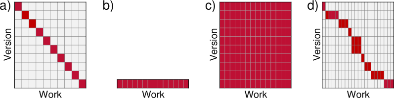
Figure 1: Types of music datasets. (a) Separate-version dataset: each work recorded in a different version. (b) Single-version dataset: all works recorded in the same version. (c) Structured multi-version dataset: each work recorded in the same set of versions. (d) Mixed-version dataset: some works recorded in the same version and/or some works recorded in several versions.

Aspects of generalization. Proving and improving such general applicability poses a challenge for any empirical experiment, requiring the variety of development data to be drawn from the same distribution of examples as the variety of intended application cases. To frame our MPE problem in terms of Empirical Risk Minimization (ERM) [9], we assume the existence of an unknown joint probability $P(x,y)$ between the input $x\in X$ (the audio signal) and $y\in Y$ (the pitches). Our goal is to estimate a function $\hat{y}\!=\!f_{\theta}(x)$ that approximates $P(y|x)$. The difference between $y$ and $\hat{y}$ is measured using a loss $\mathcal{L}(f_{\theta}(x),y)$. Here, $f$ defines a family of functions (in our case, one of the specific network architectures described in Section III-B) and $\theta$ its parameters (estimated with a variant of the SGD algorithm with the aim to minimize $\mathcal{L}$). Since $P(x,y)$ is unknown, the risk $\mathcal{L}$ is empirically minimized over instances $(x_{i},y_{i})$ drawn from $P(x,y)$. These instances should be chosen with care to guarantee the generalization of the learned $f_{\theta}$ to the whole sets $X$ and $Y$. This generalization is often measured by separating a training, validation, and test subset—each drawn from the same $P(x,y)$. In practice, this separation poses the risk of unrealistic similarities between these subsets (e. g. the same works being present in training and test set), which must be avoided in order to prevent the models from unwanted overfitting. We therefore deal with three sources of variability: (1) the choice of the family of functions $f$ (architectures), (2) the estimation of the parameters $\theta$ (which depends not only on the optimization algorithm used but also on randomization aspects such as the initialization of $\theta$), and (3) the choice of the instances $(x_{i},y_{i})$ drawn from $P(x,y)$ (training–test splits). Most published works on MPE only study the influence of (1), claiming $f$ to be “state-of-the-art” without considering the influence of (2) and (3). In this paper, we reflect on such generalization issues for MPE, thus emphasizing the importance of (2) and (3), which can drastically change conclusions related to (1).

Scenario. To this end, we focus on Western classical music scenarios, which we consider interesting for two main reasons: First, musical scores and recorded performances highly correspond to each other regarding pitch information, which allows for generating annotations in a semi-automatic way (see Section II). Second, musical compositions are usually accessible in various performances, which constitute separate interpretations and acoustic renderings, influenced by the performer style, recording conditions, audio mastering, and other aspects. We denote a specific setting of performers, instruments, and recording conditions as a version: Usually, tracks on a CD (or compilation) are homogenous regarding these version aspects. In particular, this is the case for the individual works (movements) of work cycle (a multi-movement composition such as a sonata or string quartet). Previous research in MIR showed that not reflecting version or work similarities across training and test sets can lead to severe evaluation problems [10], resulting in overfitting to either recording conditions (the so-called “album effect” in genre classification [11]) or to musical characteristics of works (a “song effect” for local key estimation [12]).

Multi-version datasets. The presence or absence of several such versions characterizes different types of MPE datasets (see Fig. 1): Ideally, each work in a dataset is rendered in a different version (Fig. 1a). In practice, however, many datasets are homogenous regarding version characteristics (single version, Fig. 1b): Examples are Bach10 [13], TRIOS [14], PHENICX-Anechoic [15], or the Choral Singing Dataset [16]. In contrast, dedicated multi-version datasets (Fig. 1c) such as the Schubert Winterreise Dataset [17] provide several versions of all works in a comprehensive fashion. Many datasets of classical music, however, are unstructured in this respect (Fig. 1d), partially providing multiple works in the same version and/or multiple versions of the same work. This is the case for the MusicNet dataset [18], a great resource of 330 license-free audio files with pre-synchronized pitch annotations. MusicNet crucially stimulated the advancement of MPE beyond the piano scenario [19, 20, 21] and has become the benchmark dataset for beyond-piano AMT. For this reason, we consider it as our central evaluation scenario. As one main contribution, we go beyond the standard test set used for MusicNet and investigate model generalization by systematically comparing different training–test splits, drawing inspiration from cross-version experiments as performed in [12]. To this end, we consider the Schubert Winterreise Dataset [17] as a second dataset that allows to systematically study generalization across versions, works, or both. We finally compile a larger and more diverse dataset from several source datasets with different instrumentations, thus providing more insights into the robustness of the models.

Deep-learning methods. Such aspects of robustness and generalization are particularly important for MPE systems based on supervised deep learning, which has become the de-facto standard approach [5, 19, 6, 3]. U-net models led to major advancements in MPE [20, 22, 23] and, recently, the inclusion of self-attention components [3, 21] or multi-task strategies [20, 22] into U-nets showed further success. In this paper, we take up such network architectures based on U-net and self-attention components [3] and propose several extensions. While many of the mentioned studies claim state-of-the-art MPE results, improvements usually happen in small increments, especially for beyond-piano scenarios. We questions this practice by addressing the results’ dependency on randomization effects (initialization of parameters) and the models’ generalization capabilities (training–test splits, cross-version and cross-dataset experiments).

Main contributions: In summary, this paper focuses on the frame-wise, instrument-agnostic, polyphonic music transcription task (MPE) beyond the piano-solo scenario using several public datasets, most importantly MusicNet [18] and the Schubert Winterreise Dataset [17]. Our main contributions are the following: (1) We realize an enhanced U-net architecture with self-attention at the bottleneck layer—loosely inspired by [3]—and propose several modifications to this architecture including self-attention for skip connections, replacement of self-attention with recurrent layers, and multi-task training with additional degree-of-polyphony estimation at the bottleneck layer. (2) We compare variants of these models in different sizes among each other and to various baseline architectures, obtaining state-of-the-art results for several model variants. (3) We study the stability of results across different training runs and find that the training substantially depends on randomization effects, which questions previous conclusions about model superiority. (4) Inspired by this finding, we systematically compare the results’ dependency on the choice of the training–test split and investigate generalization across works, versions, and datasets. (5) Finally, we propose a best-practice evaluation strategy for MusicNet and other datasets, which is shown to be crucial for measuring progress in the MPE task with data-driven systems.

The remainder of the paper is organized as follow: Section II discusses relevant datasets. Section III summarizes related work on MPE methods and sketches the models used in this paper. Section IV presents the experiments. Section V discusses our findings. Section VI concludes the paper.

II Scenario and Datasets

TABLE I: Audio datasets with multi-pitch annotations used in this paper. ¹ For work cycles, each movement is counted as a work. ² Versions per work for multi-version datasets.

ID	Dataset Name	Style / Instrumentation	Pitch annotation strategy	Mix Tracks	Works1	Versions2	hh:mm
MuN	MusicNet [18]	Chamber music (piano, strings, winds)	Aligned scores	330	306	1 up to 3	34:08
SWD	Schubert Winterreise [17]	Chamber music (piano, solo voice)	Aligned scores	216	24	9	10:50
Tri	TRIOS [14]	Chamber music (piano, strings, winds)	Multi-track	5	5	1	0:03
B10	Bach10 [13]	Chamber music (violin, winds)	Multi-track	10	10	1	0:06
PhA	PHENICX-Anechoic [15]	Symphonic (orchestra)	Multi-track	4	4	1	0:10
CSD	Choral Singing Dataset [16]	A cappella (choir)	MIDI-guided performance	3	3	1	0:07

This section specifies the task approached by this paper and discusses the datasets used in this work (see Table I).

II-A Task Definition

This paper deals with the task of MPE or frame-wise polyphonic music transcription [1], i. e., we aim for detecting the frame-wise activity of all pitches as indicated by a musical score, yet over the time axis of a recorded performance (audio). While this task is only a first step towards notation-level transcription [1], the resulting piano-roll representation (red lines in Fig. 2) is well-interpretable and constitutes a direct link to symbolic representations such as MIDI. As opposed to higher-level aspects of music notation (pitch spelling, instrument assignment), the MPE subtask constitutes a more signal-level problem and is closely related to multiple-fundamental-frequency or Multi-F0 estimation (MFE), which aims for extracting the detailed frequency trajectories of all harmonic sources in an audio signal, usually involving a sub-semitone frequency resolution (around 10 cents) and a fine-grained time resolution (around 10 ms). Beyond the resolution, pitch differs from F0 through being a perceptual phenomenon. It is not straightforward to map F0 to pitch in the presence of acoustic phenomena such as inharmonicities or vibrato (amplitudes up to several semitones in classical singing [24]).

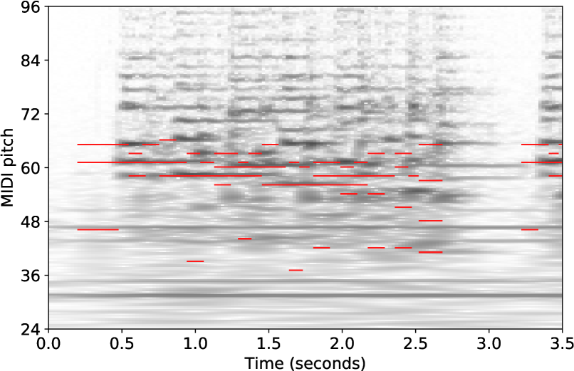
Figure 2: Id. 2382 from the MusicNet dataset, a recording of Beethoven’s string quartet op. 130, second movement, Presto. Log-compressed constant-Q transform (gray) and multi-pitch annotations (red) for the beginning.

II-B Multi-Pitch Datasets

Successful training of high-capacity neural networks requires large amounts of annotated data. The limited availability of large datasets constitutes a major issue for MPE [1]. Since a fully manual annotation is tedious and requires a high degree of expert knowledge, several strategies were proposed, as summarized by Su et al. [25].

Annotation strategies. One strategy involves the use of MIDI-fied pianos for simultaneously generating audio and annotations, leading to piano datasets such as SMD [26], MAPS [27], or MAESTRO [7]. While this is limited to few instruments (piano, organ, synthesizers), Su et al. proposed an expert-in-the-loop approach to apply this strategy to non-piano music by re-playing parts on a MIDI instrument [25].

Another strategy to go beyond the piano-solo scenario involves multi-track recordings to generate annotations with a monophonic F0-tracker on individual tracks. This was done, e. g., for MedleyDB [28] and leads to multi-F0 rather than multi-pitch annotations (see Section II-A). Since the conversion of F0 to pitch is non-trivial, we do not use MedleyDB.

However, multi-track recordings can also be used to simplify the manual pitch annotation process [13, 14, 15], which led to several small yet carefully-annotated MPE datasets such as Bach10 (B10) [13], TRIOS (Tri) [14], or PHENICX-Anechoic (PhA) [15] (all $\leq$10 tracks, see Table I). In other cases, the process is reversed: E. g., for the Choral Singing Dataset (CSD) [16], the annotation (MIDI file) served as a guideline for the singers (together with a conductor video), which were recorded in groups according to the four musical parts. All these datasets have high-quality pitch annotations but were recorded specifically for research purposes in homogenous conditions and, therefore, constitute “single-version” datasets in the sense of Fig. 1b.

Annotation by score aligment. As an alternative strategy, machine-readable scores can be exploited to generate pitch annotations, either using automated music synchronization [29] or relying on weakly-aligned training strategies using, e. g., the CTC loss [30]. For genres such as pop music, scores are rarely available or only roughly correspond to the pitch content of the recording, thus only serving as “weak labels” [1]. This is different for professional recordings of classical music, where a one-to-one correspondence between score and audio can be assumed (up to structural differences).

Such score–audio pairs of classical music were considered to generate the MusicNet (MuN) dataset [18], an excellent resource of 330 license-free audio files with pre-synchronized pitch annotations that crucially stimulated the advancement of MPE [19, 20, 21]. MuN is a very challenging dataset for MPE, yielding consistently and substantially worse results (F-measure below 75% [20]) across all studies compared to piano datasets such as MAPS or MAESTRO (up to 90% F-measure [7]). We suspect three central reasons for this: First, as reported by several authors [3, 31], the annotations in MuN are generated with automated synchronization, which leads to inaccuracies or synchronization errors (shifts) that especially affect frames around the start and end of notes or works in fast tempo (see Fig. 2 for the latter). Second, MuN contains license-free audio files, which are often digitized from old records suffering from audio artifacts (in contrast to commercial recordings) and stem from a variety of sources, interpreters, and acoustic conditions (in contrast to the quite homogenous conditions of MAPS or MAESTRO). Third, MuN captures a great variety of instruments, genres, and composers, which are, however, quite imbalanced in the dataset (see [18]): It mainly contains chamber music for solo instruments (piano, violin, cello), with piano solo accounting for almost half the total audio length, but also works for up to six players involving piano, strings, and wind instruments. Regarding composers, there is also an imbalance, with Beethoven accounting for more than half of the audio content. These imbalances hamper generalization to the underrepresented scenarios. In this paper, we investigate the latter issue by systematically comparing different training–test splits on MuN, thereby drawing inspiration from cross-version experiments as performed in [12]. In this context, it is important to note that MuN is a mixed-version dataset as indicated by Fig. 1d: Most often, several movements (usually two to five) of a work cycle are included (in a specific version), but it is unknown whether different cycles stem from the same version (are recorded under the same conditions). Some works also exist in multiple versions. However, the dataset is neither structured nor comprehensive in this respect. Therefore, we further consider the Schubert Winterreise Dataset (SWD) [17] as a comprehensive multi-version dataset (Fig. 1c), which allows to systematically study generalization across versions, works, or both, while being restricted to a smaller and more homogenous set of musical works (the 24 songs of the Winterreise cycle). SWD comprises nine recorded performances (two free and seven commercial versions), scores, and pitch annotations, generated with a synchronization algorithm [29].

We finally compile a larger and more diverse dataset from several source datasets with different instrumentations (Table I), allowing for insights into model behavior for a broader range of annotation strategies and music scenarios.

III Technical Methods

This section summarizes relevant deep-learning approaches to MPE focusing on the beyond-piano case (Section III-A) and, in particular, on models tested on MuN. We then present the architectures considered in this paper (Section III-B).

III-A Previous Models

Traditional approaches to MPE typically rely on matrix factorization techniques [4, 32]. Over the last years, deep-learning approaches led to major improvements for this task [5, 19, 6, 3]. In this context, a variety of different network architectures such as a Recurrent Neural Network (RNN) [33], a Convolutional Neural Network (CNN) [5, 19], or their combination [6, 7] were proposed. Kelz et al. [5] showed that a CNN performs on par with dense or recurrent architectures while having fewer parameters—once it is used with a suitable input representation. A particular input representation is the Harmonic Constant-Q Transform (HCQT), where CQTs in harmonic frequency ratios are stacked depth-wise such that harmonic relationship is represented along the channel dimension [34]. Using HCQT as input to a CNN has shown success for MFE [34] and MPE [30]. For these reasons, we base our methods on convolutional blocks and use an HCQT as input representation. As a major advancement, U-net models [35] were shown to improve performance of AMT [20, 3, 22, 23, 36, 21] and other MIR tasks [37, 38]. More recently, the inclusion of self-attention components into U-nets [3, 21] and other models [39] was applied successfully to MPE. Most of our architectures rely on the U-net paradigm, enhanced with self-attention components as in [3] and other extensions.

Multi-task strategies. While the models mentioned above are usually trained on the MPE task in isolation, major success was reported when proceeding to multi-task settings, most prominently the onset-and-frames approach [6, 7, 39]. However, this strategy is tailored to the piano-solo case (where the percussive keystrokes help to successfully track onsets) and therefore, is not generally applicable to other instruments with less prominent onsets. More recently, major advancements were reported for other, more difficult transcription tasks such as note-level [7, 8, 31, 3] and instrument-level transcription [3], where self-attention components [3] and Transformer architectures [40] have been applied successfully.

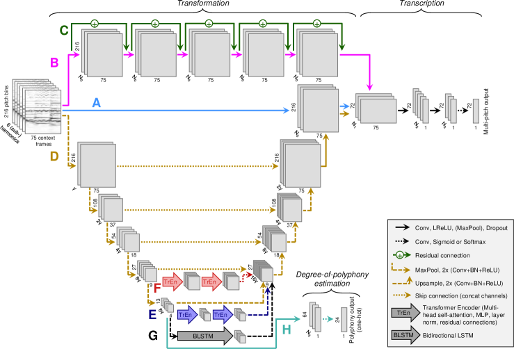
Figure 3: Overview of the model architectures used in this work. With the components (capital letters), we build several model types such as CNNs (A), Deep CNNs (B), Deep Residual CNNs (B+C), U-Nets (D), U-Nets with self-attention at the bottleneck (D+E) and also at the lowest skip connection (D+E+F), U-Nets with BLSTM (D+G), and U-Nets with polyphony estimation (D+H). See Table II for details on parameters and sizes. [Best viewed in color.]

Methods evaluated on MusicNet. Returning to the frame-level MPE task, we now discuss relevant studies that focus on Western classical music beyond the piano-solo scenario and report results on the MuN dataset. By introducing MuN, Thickstun et al. propose several baseline methods working on raw audio input. Building on this, they further propose CNN-based architectures and data augmentation strategies (tuning and transposition) obtaining substantial improvements [19].

Wu et al. [20] employed a U-Net with enhancement (atrous spatial pyramid pooling) for “semantic segmentation”. As input representation, they consider a frequency–periodicity representation also including harmonics, similar to the HCQT idea. They achieve an F-measure of 73.7%, one of the best results on MuN so far. In [3], they extend the task towards multi-instrument transcription, enhancing the model of [20] with self-attention at the bottleneck, with improved results for instrument-wise transcription but similar results on MPE.

Another U-net-based MPE approach was proposed by Pedersoli et al. [23], who investigate the “pre-stacking” of a U-Net to different CNNs. Here, the U-Net serves as a “transformation network” followed by the CNN as a “transcription network,” which they found to be more effective than just increasing depth or width. In this paper, we take up their idea of pre-stacking the U-net. Cheuk et al. [36] consider two U-Nets, one for transcription and one for spectrogram reconstruction, connected with Bidirectional LSTM components and a reconstruction loss. Aiming towards better model generalization, they combined the reconstruction paradigm with virtual adversarial training [21]. To put a semantic meaning to the bottom part (bottleneck), some authors train the U-net in a multi-task fashion [41, 22] by extracting a voice activity estimate from the bottleneck, applied for monophonic pitch estimation of the predominant melody [41] or the bass line [22].

Beyond the U-net, further architectures were tested on MuN. Steiner et al. [42] test echo-state-networks, a kind of RNN. Gardner et al. [31] approach multi-instrument transcription tasks with Transformers. The obtained promising results, which dropped when using cross-dataset evaluation. Investigating MuN, they point to synchronization inaccuracies and labeling issues—aspects that we discuss later in this paper.

III-B Proposed Models

For the experiments in this paper, we consider a variety of deep-learning approaches as summarized in Fig. 3. Since describing all details in a comprehensive way is not possible here, we restrict ourselves to describing the central concepts and refer to our source code for implementation details. All model variants share a convolutional post-processing stage as proposed by [30], taking up the idea of a transformation and a transcription part [23], which are trained together. As input, we use a log-compressed HCQT with five harmonics and one subharmonic, comprising six octaves (C1–C7, or MIDI pitches 24–96) with three bins per semitone, resulting in 216 pitch bins, and using librosa’s tuning estimation for adjusting bin frequencies. We rely on a sample rate of 22.05 kHz and an HCQT hopsize of 512 samples, resulting in a frame rate of 43.07 Hz. All models operate on input patches of 75 frames (center frame plus 37 context frames to each side) corresponding to 1.74 s of audio, processed by layer normalization, and predict the pitch activities of the center frame.

CNN architectures. Our basic model variant is a CNN with five layers (Fig. 3 A, blue path) as used in [30] for MPE and in [43] for pitch-class estimation. The first layer performs prefiltering (compression of the harmonics/channels) and preserves the input size, followed by reduction to pitches (one bin per semitone), temporal reduction, and a channel reduction. The model size (number of parameters) can be adjusted by increasing the width (number of channels/kernels) in each layer, specified by N₀, N₁, N₂, N₃ (see Table II for concrete realizations). All layers use 2D-convolutions followed by LeakyReLU activations (slope 0.3), 2D-max-pooling, and dropout (rate 0.2). The final layer has a sigmoid activation since the models are trained with Binary Cross-Entropy (BCE) loss. For the following model variants, we only replace the first (prefiltering) layer by more complex components, keeping all subsequent layers identical to CNN.

DCNN and DRCNN architectures. Inspired by [43], we realize a Deep CNN (DCNN) variant by replicating the pre-filtering layer five times (Fig. 3 B, magenta path). We enhance this variant with additive skip connections (residual connections) around the pre-filtering layers, resulting in a Deep Residual (DRCNN) architecture inspired by the ResNet [44] (Fig. 3 B+C, magenta and green paths).

Unet architectures. Due to its frequent and successful use for MPE, we consider the U-net [35] as basis for our further architectures. We adopt the idea of pre-stacking a U-net [23] to our post-processing CNN (Fig. 3 D, golden path). After an initial double-convolution layer with batch normalization (BN) and ReLU activation, we employ four downsampling steps (max-pooling by a factor of two) followed by the double-convolution module, and four upsampling steps followed by double-convolution. We realize the skip connections by concatenating channels from the downsampling and upsampling part. The width (channels) can be controlled with a parameter $\gamma$ leading to U-nets in different sizes (see Table IId).

SAUnet and SAUSnet (with self-attention components). Inspired by [3], we consider an extension of the U-net with self-attention at the bottom part (bottleneck) denoted as Self-Attention U-net (SAUnet, Fig. 3 D+E, golden and navy paths). As opposed to the memory-flange self-attention in [3], applied to patches of the downsampled representation via raster-scan, we simply flatten the time and frequency axes and use two Transformer encoder blocks as proposed by [40]. Such a block consists of a multi-head self-attention and a fully connected network (multi-layer perceptron). Both blocks are followed by dropout and layer normalization and applied in a residual fashion (output added to the previous input). As in [40], we add absolute positional encodings as a combination of sine and cosine functions in order to inform the self-attention about the sequence order. In accordance with [40], we obtained similar results when using learned positional encodings instead. We always use eight attention heads so that the embedding dimension is determined only by the U-net size $\gamma$. The number of hidden nodes is parametrized by $\lambda$. Among the different sizes listed in Table II, we consider the SAUnet:L with roughly eight million parameters as most similar to the model presented in [3]. We further propose a modification to this architecture by introducing self-attention for the lowest skip connection (SAUSnet, Fig. 3 D+E+F, golden, navy, and red paths), using the same Transformer encoders as described above. Beyond this paper’s results, we also experimented with self-attention at higher skip connections obtaining worse results.

BLUnet (with recurrent components). Since the attention mechanism has been proposed for effectively processing sequence data [40], we also test a recurrent variant where we replace self-attention by Bidirectional Long-Short-Term Memory (BLSTM) component (BLUnet, Fig. 3 D+G, golden and black paths), the more common technique to capture sequence information. In this case, the parameter $\lambda$ denotes the number of hidden units in the BLSTM layer (see Table II).

PUnet (with polyphony estimation). Finally, we consider a multi-task strategy to enforce a semantic meaning of the lowest U-net layer (bottleneck). We draw inspiration from [41, 22], where the bottleneck is trained with an auxiliary task: predicting the activity (voicing) in monophonic pitch estimation scenarios. Since inactive frames are rare in our multi-pitch scenario, we propose an alternative: As an auxiliary task, we predict the local degree of polyphony, i. e., the number of active pitches in the center frame (0–23), which turned out to be a useful side information for MPE [13, 45]. We derive this information from the bottleneck of the U-net, post-processed by a small, two-layer CNN with 24-class softmax output. This variant is called the Polyphony U-net (PUnet, Fig. 3 D+H, golden and aquamarine paths).

IV Experiments and Results

This section presents our comprehensive experiments and results. We first detail the experimental procedure (Section IV-A). Next, we compare the performance of our architectures in varying size (number of parameters) on MuN (Section IV-B). We report on the reliability of these results and investigate different test subsets of MuN (Section IV-C). Then, we perform a systematic cross-version study on SWD (Section IV-D). Finally, we test generalization to other scenarios by compiling a mixed dataset (Section IV-E).

IV-A Experimental Protocol

We now describe the experimental protocol to train and test our models for MPE. The details of the dataset splits are discussed later when presenting the respective results.

Training procedure. For training our models, we feed mini-batches of 25 HCQT excerpts as input, each having a size of 75 context frames, 216 pitch bins, and 6 (sub)-harmonics (see Section III-B for details) with slight logarithmic compression, along with the corresponding multi-pitch annotations for the center frame. We sample these excerpts from the full tracks’ HCQT at regular intervals and adjust the stride parameter (hop size) such that the training set comprises roughly 95k training examples (3800 batches) and 9k validation examples (360 batches). All these examples are processed for one epoch to be finished. We train the model for a maximum of 100 epochs with the AdamW optimizer [46], a stabilized version of the Adam optimizer using decoupled weight decay regularization, with an initial learning rate 0.001. For scheduling, we halve the learning rate if the validation loss plateaus for five epochs. After twelve non-improving epochs, we perform early stopping and use the best-performing model (with respect to the validation loss) for testing. In practice, we rarely need more than 20 epochs to reach convergence; only the simpler models (CNN and DCNN) require more epochs (up to 50). As criterion, we compute the BCE loss between pitch predictions and targets. For the PUnet model, we also calculate the Categorical Cross-Entropy (CE) loss for the degree-of-polyphony output (compare Fig. 3) and sum the two losses. To have the losses in a similar order, we scale the CE loss with a factor of 0.04 (empirically tested, not further optimized).

TABLE II: Comparison of network architectures, trained on the dataset MuN and tested on the test set MuN-10_a.

Model	Param.	Channels	$\gamma$	$\lambda$	Eval. Measures (%)
Type:Size	$/10^{3}$	N0,N1,N2,N3			P	R	F	AP
(a) CNN (Fig. 3 A)
CNN:XS	48	20,20,10,1	–	–	69.0	61.4	64.5	69.3
CNN:S	603	100,100,50,10	–	–	68.7	67.8	68.0	73.2
CNN:M	1,813	​250,150,100,100	–	–	71.0	71.5	70.9	75.3
CNN:L	2,467	​280,180,120,100	–	–	70.4	71.7	70.7	75.0
(b) DCNN (Fig. 3 B)
DCNN:S	408	20,20,10,1	–	–	84.0	42.7	55.4	76.7
DCNN:M	1,602	40,40,30,10	–	–	68.2	80.9	73.8	78.6
DCNN:L	4,815	70,70,50,10	–	–	78.2	71.0	72.8	78.2
(c) DRCNN (Fig. 3 B+C)
DRCNN:S	408	20,20,10,1	–	–	82.1	49.6	61.3	77.0
DRCNN:M	1,602	40,40,30,10	–	–	70.3	78.2	73.9	78.5
DRCNN:L	4,815	70,70,50,10	–	–	70.1	78.2	73.6	78.2
(d) Unet (Fig. 3 D)
Unet:S	882	64,30,20,10	8	–	72.1	75.3	73.3	77.8
Unet:M	1,655	128,100,80,50	8	–	71.9	76.5	73.9	78.0
Unet:L	4,552	128,150,100,80	16	–	73.9	74.1	73.8	79.0
Unet:XL	14,252	​128,180,150,100	32	–	71.9	77.9	74.6	79.1
(e) SAUnet (Fig. 3 D+E)
SAUnet:M	1,180	64,30,20,10	8	​1024	72.4	73.3	72.6	77.0
SAUnet:L	7,983	128,80,50,30	16	​8192	73.7	76.6	75.0	79.8
SAUnet:XL	10,093	​128,200,150,150	16	​8192	71.5	77.6	74.2	78.8
SAUnet:XXL​​	23,439	​128,200,150,150	32	​8192	72.4	76.3	74.0	78.6
(f) SAUSnet (Fig. 3 D+E+F)
SAUSnet:M	1,213	64,30,20,10	8	512	74.0	70.0	71.8	76.9
SAUSnet:L	8,115	128,80,50,30	16	​4096	75.8	71.6	73.4	79.0
SAUSnet:XL	14,436	​128,200,150,150	16	​8192	73.7	77.1	75.1	79.6
SAUSnet:XXL​​​	32,371	​128,200,150,150	32	​8192	70.9	76.7	73.4	77.7
(g) BLUnet (Fig. 3 D+G)
BLUnet:M	1,343	64,30,20,10	4	208	73.4	72.0	72.4	77.1
BLUnet:L	9,649	128,80,50,30	8	416	71.8	76.9	73.6	78.5
BLUnet:XXL​	22,376	​128,200,150,150	16	832	73.2	73.6	73.1	77.9
(h) PUnet (Fig. 3 D+G)
PUnet:M	1,680	128,100,80,50	8	–	75.1	74.0	74.3	79.4
PUnet:L	4,643	128,100,80,50	16	–	72.7	75.8	74.0	78.9
PUnet:XL	14,598	​128,180,150,100	32	–	72.8	75.8	74.1	79.1

Data augmentation. To improve model generalization, we use data augmentation during training (not validation) on the pre-computed HCQT excerpts (in contrast to [19], which employs augmentation on the raw waveform). As augmentation strategies, we employ transposition by shifting the HCQT by a random amount of steps (up to $\pm 5$ semitones), filling the gaps with zeros, and shifting the labels accordingly. We further employ tuning augmentation by shifting for $\pm 1$ CQT bin (1/3 semitone) or by $\pm 0.5$ bins (averaging neighboring bins), thereby preserving the labels. Moreover, we add Gaussian noise to all HQCT values with a standard deviation of $10^{-4}$. To simulate different timbral characteristics, we apply the RandomEQ technique presented in [22] with parameters $\alpha\in\{1,\ldots,21\}$ and $\beta\in\{1,\ldots,216\}$ (for details, see [22]). In preliminary experiments, we found data augmentation to have a small but consistently positive effect on test performance.

Evaluation measures. To assess the effectiveness of our models, we predict multi-pitch estimates for all test files with a dense sampling (stride of 1 as in [18]), i. e., all test frames are predicted and evaluated, at a frame rate of 43.07 Hz. As evaluation measures, we compute the Precision (P), Recall (R), and F-Measure (F). To binarize model outputs, we use a global prediction threshold of 0.4 as in [19] instead of tuning the threshold on the validation set (as done in [20]). Hypothesizing that a more general, threshold-independent measure is better suitable to estimate model quality, we also compute the Average Precision (AP) score, which corresponds to the Area under the Precision–Recall curve, a concept similar to the Receiver-Operator-Characteristics (ROC) curves. As in [18, 19], we use AP as our primary evaluation measure. All measures reported in this paper are class-wise micro-averages (all active bins contribute equally irrespectively of the pitch) and track-wise macro-averages (all test tracks contribute equally irrespectively of their length), given in percent.

TABLE III: Different test subsets of the MusicNet dataset. ^∗ See footnote 12 for handling Bach’s Well-tempered Clavier.

		Test set tracks (MusicNet ID, movement no. and tempo)
Composer	Work	MuN-3 / MuN-10	MuN-10a	MuN-10b	MuN-10c	MuN-10full
Bach	Well-tempered Clavier Book 1	2303, 5-Prel. D maj	2303, 5-Prel. D maj	2302, 5-Fugue D maj	2310, 15-Prel. G maj	2302–2305 ∗
Mozart	Serenade K 375	1819, 4-Menuetto	1819, 4-Menuetto	1818, 3-Adagio	1817, 2-Menuetto	1817–1819
Beethoven	String Quartet No. 13 Op. 130	2382, 2-Presto	2382, 2-Presto	2383, 3-Andante	2381, 1-Adagio-Allegro	2381–2384
Bach	Cello Suite No. 4 BWV 1010	2298, 6-Gigue	2298, 6-Gigue	2293, 1-Prelude	2296, 4-Sarabande	2293–2298
Bach	Violin Partita No. 3 BWV 1006	2191, 6-Bourree	2191, 6-Bourree	2186, 1-Preludio	2186, 1-Preludio	2186, 2191
Beethoven	Piano Sonata No. 30 Op. 109	2556, 2-Prestissimo	2556, 2-Prestissimo	2557, 3-Gesangvoll	2555, 1-Vivace-Adagio	2555–2557
Beethoven	Wind Sextet Op. 71	2416, 3-Menuetto	2416, 3-Menuetto	2415, 2-Adagio	2417, 4-Rondo-Allegro	2415–2417
Beethoven	Violin Sonata No. 10 Op. 96	2628, 3-Scherzo	2629, 4-Poco allegretto	2627, 2-Adagio espr.	2626, 1-Allegro mod.	2626–2629
Schubert	Piano Sonata D 958	1759, 3-Men. Allegro	1759, 3-Men. allegro	1758, 2-Adagio	1757, 1-Allegro	1757–1760
Haydn	String Quartet Op. 645	2106, 3-Men. Allegretto	2106, 3-Men. allegretto	2105, 2-Adagio cant.	2104, 1-Allegro mod.	2104–2106

IV-B Evaluating Model Architectures and Sizes

As our first experiment, we now evaluate all models proposed in Section III-B on the MuN dataset (results listed in Table II). To this end, we use the 10-track test set MuN-10_a as specified in Table III (we discuss the choice of the test set in the following section) and further 27 tracks for validation. For each model type, we realize different sizes by adjusting the parameters N${}_{0},\ldots,\,$N₃ and, if applicable, $\gamma$ and $\lambda$ (see Section III-B) with resulting model sizes from roughly 48k (CNN:XS) to 32M (SAUSnet:XXL) parameters. We consider the self-attention U-net, SAUnet:L, with roughly 8M parameters, to be most similar to the well-performing model of [3]. In addition, Fig. LABEL:fig:modelsizes visualizes the AP values for the models listed in Table II, with models of the same type connected by lines (we later discuss the additional disconnected points).

Standard CNNs. Let us first regard the results of the shallow CNN models (Table IIa). For the smallest model CNN:XS, which corresponds to the one tested in [30], we obtain a reasonable result of AP=69.3%. By widening this model (using more channels), we can substantially improve its performance up to AP=75.3%. We reach a peak at a model size of roughly 1.8M parameter before the performance slightly drops (compare Fig. LABEL:fig:modelsizes). A similar “peaking” behavior can be found when we increase the model depth (DCNN, Table IIb) and when adding residual connections to this deeper CNN (DRCNN, Table IIc). Compared to the shallow CNN, the deeper models achieve superior results of AP$>$78%, suggesting that a certain depth is necessary for good performance.

U-nets. Looking at the U-net models (Table IId), we observe similar performance for the smaller model sizes (Unet:S and Unet:M). Nevertheless, it seems that using a U-net structure allows to substantially increase the model size up to 14M parameters (Unet:XL) to achieve improved results of AP=79.1%. Enhancing the U-net with self-attention modules at the bottom (SAUnet, Table IIe), we find even better results up to AP=79.8% for SAUnet:L, the model similar to [3]. Interestingly, performance drops for the larger variants of this model (SAUnet:XL and SAUnet:XXL), again suggesting that an ideal size exists for this model as observed above.

Proposed extensions. Regarding our own extensions of the models, let us first discuss the SAUSnet models (Table IIf), where we added self-attention modules also to the U-net’s lowest skip connection (in addition to the bottleneck). These models also perform well with the peak result of AP=79.6% at a slightly larger size of roughly 14M parameters. Replacing bottleneck self-attention with recurrent modules (BLUnet, Table IIg), we obtain worse results than for SAUnet. Finally, let us turn to the multi-task model PUnet (Table IIh), where we constrain the bottleneck by training on degree-of-polyphony estimation. These models show good performance comparable to the standard U-nets. However, the smallest model with polyphony estimation (PUnet:M) obtains AP=79.4%, being superior to the equally-sized Unet:M with AP=78.0%, suggesting that multi-task training can help for smaller models. Summarizing these results, we can achieve well-performing MPE systems with any of our convolutional approaches. To boost performance, a certain model depth seems to be necessary; we obtained further improvements by using U-net architectures and additional enhancement strategies.

Reliability of results. At this stage, we want to point out that differences in AP (and other evaluation measures) are usually small—often less than one percentage point. This raises the question of the results’ stability. We therefore re-run some selected model configurations. Since any type of stochastic gradient descent depends on randomization, we expect at least slightly different results. In our case, randomization is involved at four stages of model training: The random initialization of model parameters $\theta$, the random order of training samples and batches in an epoch, the random parameter choices involved in the data augmentation, and the randomness in dropout layers.

We plot the AP values from the additional re-runs as extra isolated points into Fig. LABEL:fig:modelsizes (same marker types at the same horizontal positions stem from identical models). The result is remarkable: For our best model from Table II (SAUnet:L), each re-run leads to worse results, down to AP=77.5%. For the second best model, SAUSnet:XL, re-runs produce worse results as well. In contrast, one re-run of Unet:XL achieves a top result of AP=79.9%. In general, the variation in AP between runs reaches up to more than two percentage points, which is clearly larger than most performance differences between model architectures and sizes. This not only questions the usefulness of the self-attention components and the other U-net enhancements but also the role of model architecture at all: We cannot even claim U-net-based models to be superior to DCNN or DRCNN architectures from this experiment. However, this does not allow for the opposite conclusion (that these architectures are not better)—we just cannot safely conclude anything on model superiority from this experiment.

IV-C Investigating Model Generalization

To approach this problem, we reconsider several components of our procedure. Hypothesizing that a larger training and validation set may stabilize model performance across runs, we increase their size by a factor of 2.5 using denser HCQT sub-sampling (smaller stride), raising the number of training examples from roughly 95k to 236k and the number of validation examples from roughly 9k to 23k.

Larger training set. Table IVa shows the results of this adapted experiment for selected models. For the three SAUnet:L runs, we observe performance to stabilize (only 0.4 percentage points variation) and to improve (AP$>$80% for two runs). This improvement is confirmed for SAUSnet:XL and PUnet:XL, which surpass their performance with less training data in Table II. However, the runs of Unet:XL in Table IV show a variation of more than three percentage points in AP, indicating that an increase of training data is not sufficient for safely excluding negative randomization effects.

TABLE IV: Results with larger training set (denser sampling) and (partially) re-runs, evaluated with different test sets.

Model	Param.	Run	Eval. Measures (%)
Type:Size	$/10^{3}$		P	R	F	AP	Acc
(a) Test set MuN-10a (Section IV-B)
Unet:XL	14,252	1	68.3	80.0	73.3	77.2	58.3
		2	71.9	77.3	74.2	78.3	59.3
		3	76.0	74.9	75.2	80.3	60.6
SAUnet:L	7,983	1	75.8	73.4	74.3	80.0	59.7
		2	74.6	76.6	75.4	80.1	60.8
		3	74.5	74.7	74.4	79.7	59.5
SAUSnet:XL	14,436	–	75.3	76.3	75.6	80.2	61.1
PUnet:XL	14,598	–	75.1	75.6	75.1	80.6	60.4
(b) Test set MuN-10 [19, 20]
Unet:XL	14,252	1	74.8	73.1	73.7	78.8	58.7
		2	73.6	75.3	74.2	79.2	59.4
		3	73.2	78.1	75.5	80.4	61.0
SAUnet:L	7,983	1	72.2	76.8	74.2	79.0	59.7
		2	72.9	72.7	72.6	77.4	57.4
		3	73.1	76.0	74.3	79.5	59.7
SAUSnet:XL	14,436	1	69.8	79.4	74.1	78.7	59.1
		2	72.6	78.0	75.0	79.6	60.4
		3	71.2	78.0	74.2	78.8	59.3
PUnet:XL	14,598	–	75.6	74.7	74.9	80.6	60.2
(c) Test set MuN-3 (90s) [18, 19]
Unet:XL	14,252	–	66.3	76.4	70.8	74.6	55.4
SAUnet:L	7,983	1	74.5	64.1	68.8	75.0	53.3
		2	74.1	74.0	74.0	78.4	59.2
		3	74.8	70.5	72.5	78.0	57.6
SAUSnet:XL	14,436	–	74.8	71.7	73.2	77.5	58.4
PUnet:XL	14,598	–	74.5	69.4	71.8	77.3	56.5
(d) Test set MuN-10b (slow movements)
SAUnet:L	7,983	–	75.2	82.1	78.5	83.0	64.8
(e) Test set MuN-10c (fast movements)
SAUnet:L	7,983	–	75.0	72.2	73.4	78.0	58.1
(f) Test set MuN-10full (all movements)
CNN:M	1,813	–	74.3	72.7	73.2	78.3	58.0
DRCNN:L	4,815	1	73.2	79.4	76.0	80.6	61.5
		2	72.3	81.1	76.2	80.8	61.8
		3	74.2	79.3	76.5	81.2	62.1
Unet:M	1,655	–	74.7	75.8	75.1	80.1	60.4
Unet:XL	14,252	–	74.5	78.3	76.2	80.9	61.8
SAUnet:L	7,983	1	76.2	74.6	75.2	80.4	60.5
		2	75.8	75.7	75.6	80.5	60.9
		3	73.6	78.7	75.9	80.7	61.3
SAUSnet:XL	14,436	–	72.0	79.8	75.5	80.1	60.9
BLUnet:L	9,649	–	76.7	72.7	74.5	79.8	59.6
PUnet:XL	14,598	1	76.2	75.5	75.7	80.8	61.1
		2	80.0	70.6	74.8	81.5	60.1
		3	76.6	76.9	76.5	81.4	62.2

MusicNet test sets in related work. As another critical aspect, we want to reflect on the test set held out from MuN for evaluation. Studying related work on MuN, we observe different test sets being used (compare Table III). In the original paper [18] and a follow-up work by its authors [19], a test set of three tracks (MuN-3) is used, restricted to the first 90 seconds (which are further subsampled), taken up by some other authors [23, 36]. In a pre-print of [19], Thickstun et al. further evaluate on a ten-track test set (MuN-10), extending MuN-3 by seven further tracks (now full tracks), with remarkable differences (AP=77.3% for MuN-3 and AP=79.9% for MuN-10 with their best model). A number of subsequent studies evaluates on MuN-10 [20, 3, 42] or an entirely different, customized training–test split [31].

A small “mistake.” In our own previous experiments (Section IV-B), we targeted a ten-track test set inspired by the literature. However, we later realized that one of our test tracks deviates from MuN-10 due to a mistyped ID (2629 instead of 2628)—this is why we named it differently as MuN-10_a (see Table III). To enable comparability with published results, we therefore re-train and test some of our models on the corrected test set MuN-10 (see Table IVb). Interestingly, we obtain worse results than in Table IVa especially for SAUnet:L and SAUSnet:XL, with the best result on MuN-10, AP=79.6%, being worse than the worst result of MuN-10_a, AP=79.7%. Only one run of Unet:XL achieves better results with AP=80.4%, and the multi-task PUnet:XL performs similar. Testing on the original test set MuN-3 from [18] (first 90s) as shown in Table IVc, we observe substantially worse results than for any ten-track test set, in accordance with [19].

Given these results, we now could follow the common practice and claim “state-of-the-art” results for several of our models, without even limiting to a particular test set or evaluation measure: On the test set MuN-10 (Table IVb), PUnet:XL (AP=80.6%) and Unet:XL in run 3 (AP=80.4%) outperform [19] (AP=79.9%) in AP, and almost all our models outperform [20] (F=73.3%) and [42] (F$<$72%) in F-measure. On the test set MuN-3 (Table IVc), our SAUnet:L in run 2 (AP=78.4%) outperforms the models from [19] (AP=77.3%), from [23] (AP=76.8%), and from [36] (AP$<$71%). However, we strongly believe that such comparisons are not meaningful given the small margin of improvement compared to the large variation of results across runs and chosen test sets.

Results in detail. Since there seems to be a substantial effect of the test set, we investigate the behavior for individual test tracks. For each of the three models from Table IVb, we take the “good” and the “bad” training run and plot the track-wise AP values in Fig. 5. For some tracks (IDs 1759, 1819, 2106, or 2303), good models are consistently but slightly better than bad models. Others achieve consistently high (IDs 2191 or 2556) or low (ID 2416) AP throughout all models and runs. Two test tracks are behaving quite differently: For ID 2298, a movement from Bach’s Cello Suite BWV 1010, the performance substantially drops for SAUnet:L. For ID 2382, a very fast movement from Beethoven’s string quartet op. 30, all models show worse results. Looking in detail at this track’s annotations (see Fig. 2 or consult https://musicnet-inspector.github.io/), we realize synchronization issues for this track, which—due to the fast tempo—result in note events being shifted to their neighbors in time. Such kind of annotation problems were highlighted for MuN by several authors. Already in the original paper [18], the authors report a quite high onset/offset error rate of 4%. Beyond that, Gardner et al. [31] found timing errors beyond 50 ms and spotted major labeling errors due to non-corresponding score–audio segments.

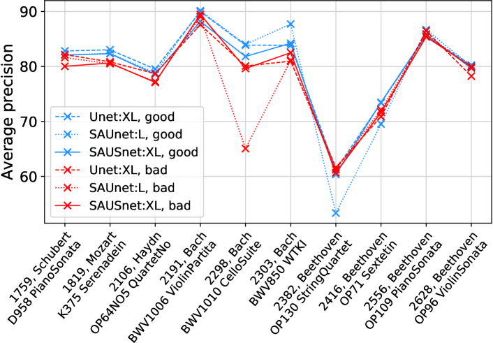
Figure 5: Results on the individual test files for MuN-10 with three good and three bad training runs.

Impact of test set choice. Beyond such labeling problems, there is another important aspect of training–test splits that we already discussed in Section I. Our small typo (ID 2629 instead of 2628) did not result in an entirely different test track being used but only in a different movement (4-Poco allegretto instead of 3-Scherzo) of the same cycle (Beethoven’s violin Sonata No. 10 Op. 96) in the same version (same performers and recording scenario) being used. This similiarity is no exception in MuN, which constitutes a mixed-version datasets as highlighted in Fig. 1d: Each cycle–version pair usually contributes several works (movements) to the dataset (organized in separate audio tracks, each with their own MuN ID). This has two consequences: First, models can overfit to the specific recording conditions of the test set, which can result in unrealistically high model performance. Second, musical aspects correlated to the movement type or tempo may influence the results, which might be one reason for the performance difference between MuN-10 and MuN-10_a.

Switching test movements. To highlight the impact of the latter issue, we now create another ten-track test set, where we replace each of the original test tracks from MuN-10 with another movement from the same cycle in the same version. Since MuN-10 contains mostly fast movements, we now take mostly slow movements, resulting in the new test set MuN-10_b (compare Table III). Retraining the model SAUnet:L with this training–test split (Table IVd), we obtain clearly improved performance of AP=83.0% (note that the performance difference between this result and any previous one is larger than the training run differences found so far). We repeat this process by taking yet another movement (now mostly fast ones as in MuN-10) resulting in the test set MuN-10_c. Here, the model SAUnet:L achieves AP=78.0% (Table IVe), which is quite similar to the result for MuN-10, suggesting that tempo-related characteristics can indeed influence model performance. This might be due to the lower average note length in fast movements, which results in synchronization errors having more influence on annotation quality.

Proposed training–test split. To address both the tempo and the generalization issues, we finally propose a stricter split where we again take the same ten work cycles as in MuN-10 but hold out all movements of each cycle for testing, resulting in 36 tracks (MuN-10_full, last column in Table III). This is beneficial for three reasons: First, the test set becomes larger, thus suppressing the impact of individual difficult (or misannotated) tracks as highlighted in Fig. 5. Second, the influence of tempo and movement characteristics is balanced out since, for each cycle, we consider a variety of movements. Third, we avoid overfitting to the specific acoustic characteristics of a recording since, for each recorded cycle, all movements are either in the training or test set. We propose this training–test split as an improved evalution strategy for MuN, which largely avoids the problems mentioned above.

The results for this split are shown in Table IVf. We observe slightly better results than for MuN-10 and somewhat worse results than for MuN-10_b, indicating that the test set MuN-10 proposed in the appendix of [19] seems to be a representative choice. However, in contrast to choosing the smaller variant of ten tracks, we now observe clearly stabilized results. For the three models with re-runs (DRCNN:L, SAUnet:L, and PUnet:XL), the variation between best and worst run is at most 0.7 percentage points, which is clearly lower than in Fig. LABEL:fig:modelsizes. Comparing model architectures on MuN-10_full confirms most of our initial findings: First, a certain depth of the network seems necessary—the shallow CNN:M performs worse than deeper models. Second, U-nets with self-attention do not prove to be better than standard U-nets of comparable size. Third, a larger U-net can outperform a smaller one. Fourth, a simple residual network (DRCNN:L) can perform equivalently to a U-net. Fifth, recurrent components are less effective than self-attention components, rather deteriorating results compared to a standard U-net. Finally, we find evidence that the multi-task strategy (PUnet:XL) is a promising technique.

IV-D Cross-Version Study: Schubert Winterreise Dataset

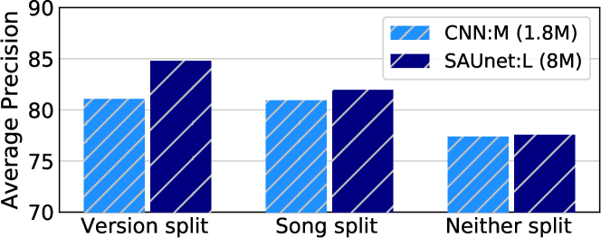
Figure 6: Cross-version study on SWD inspired by [12] for two selected models, evaluated in a version split, a song split, and an exclusive neither split.

Our previous experiments showed that work-specific aspects such as the tempo can have major influences on model performance. Yet, these experiments provided little insights about overfitting to certain versions (performance and recording conditions). To test this in a more controlled fashion, we turn to the SWD [17], a systematic multi-version dataset, which is comprehensive in the sense that each work is present in all versions and each version covers all works (Fig. 1c). The dataset has been used for a cross-version study on local key estimation [12], where models rather overfit to works (songs) than to versions. We now realize a similar cross-version study for MPE. For the version split, we use all songs in two versions for testing, two further versions for validation, and the remaining five versions for training. For the song split, we use the songs 17–24 of Winterreise in all versions for testing, songs 14–16 for validation, and songs 1–13 for training. The neither split is the intersection of the two splits.

Fig. 6 shows the results of this study for two selected models, the shallow CNN:M and the large SAUnet:L. Similar to [12], the larger model (SAUnet:L) benefits from knowing the specific songs. For CNN:M, version and song split behave similar. For the most realistic neither split, where neither the songs nor the acoustic conditions are seen by the model during training, both models suffer from a substantial drop (please note the y-scale: differences here are larger than in the previous sections). We conclude on the existence of a version effect (similar to the “album effect” in [11]) for both models and a song effect (similar to the “cover song effect” in [12]) in particular for the high-capacity model SAUnet:L.

In general, we note that performance in the realistic neither split is worse than for MuN, even though generalization is less challenging since we only deal with one composer, one work cycle, and one instrumentation. We suppose that this is due to the limited amount and variety of training data in SWD compared to MuN, which prohibits high-capacity models such as SAUnet:L from fully exploiting their potential.

IV-E Evaluation With a Mixed Dataset

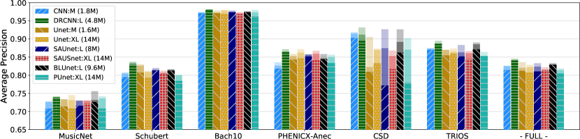
Figure 7: Generalization study on a big mixed dataset. Results of different training runs are stacked on top of each other with transparent colors.

To address the challenge of training dataset size and variety for general MPE, we finally compile a big mixed dataset using all the datasets listed in Table I as sources. For MuN, we use the test set MuN-10_a as in Section IV-B. For SWD, we employ the strict neither split as in Section IV-D. We use the full Tri dataset for testing since it comprises chamber music recordings very similar to MuN (but with very high annotation quality). All other datasets are splitted. Since the CSD is our only choir dataset, we enrich it by creating for each work also a three-part mix (once leaving out each of the four parts, respectively). The combined test set comprises 42 tracks and, thus, is comparable in size to MuN-10_full. Since the training set is much larger, we increase the sampling stride so that the number of training and validation examples is comparable to Section IV-C.

Results on the full test set. Using this combined training–test scenario, we evaluate several models, each in three runs. Fig. 7 shows the results, with the three runs’ AP values stacked on top of each other with transparent colors. Looking at the full mixed test set (rightmost bar group), we observe high AP values of 80–85% for all models. Interestingly, the residual model DRCNN:L performs best, with its worst run obtaining better AP than any run of any other model. Again, self-attention components do not improve performance of U-nets. Contrary to the findings for MuN, the recurrent components in BLUnet:L are beneficial, the smaller Unet:M is slightly better than the larger Unet:XL, and the multi-task PUnet:XL performs worse—yet on an overall high level.

Results on test subsets. Much more interesting, however, are the results for the individual test subsets. For SWD, all models show better performance using this large training set than for the corresponding neither split in Fig. 6. This confirms our previous assumption that a larger training set is beneficial here. On the contrary, the results for MuN drop by more than five percentage points compared to the corresponding results in Table IVa. Remarkably, a more diverse training set from different sources does not help for MuN (in contrast to SWD). We suppose that this is due to specific annotations characteristics of MuN, probably stemming from the synchronized annotations, which the models can effectively adapt to—as long as they only need to model training examples from MuN and not at the same time focus on singing voices or orchestral scenarios. For B10, a clean and well-annotated dataset, all models yield very good results. PhA is a more difficult one since orchestra recordings are underrepresented in our training set. The same holds for CSD since we have little choir examples for training. But here, the model performance varies dramatically across models and runs, with the simpler models CNN:M and DRCNN:L performing best. Finally, Tri is the most interesting test set since it is completely excluded from training, well-annotated, and mainly captures our central genre, classical chamber music. Despite being small (3 min overall length), results show high stability across model runs. Interestingly, the performance differences between models are similar to the full test set (though on a higher level). We conclude that Tri is a representative and useful dataset for MPE evaluation, and that residual models such as DRCNN:L seem to be most stable in cross-dataset situations.

Comparison with related work. We finally want to stress again that all these models perform well, most of them superior to previously reported results: All models outperform our previous results [30] with a smaller network similar to CNN:XS, especially for SWD. For B10, our best Unet:XL reaches Acc=87.2% as compared to a traditional method [13] with Acc$<$70% and a deep-learning approach [48] with up to Acc=85.6%. On PhA, DRCNN:L and Unet:XL reach up to AP=87.2%, as compared to our own MCTC-based results of AP=82.8% [30]. For CSD, we achieve F=86.2% with the best DRCNN:L, as compared to a CNN-based approach [16] with F$<$85% (for MFE with 100 cent resolution). Finally, on Tri, our best DRCNN:L achieves up to F=80.4% as compared to another deep-learning method [48] with F=71.8%.

V Discussion

Looking at our findings for MuN, SWD, and the mixed dataset, it remains difficult to draw a general conclusion on model architectures. Our most controlled experiment on MuN (MuN-10_full, Table IVf) indicated that U-net-based models and, in particular, the multi-task strategy PUnet are useful or at least competitive. In contradiction to this, the generalization on our big mixed dataset questioned the superiority of large U-nets in favor of the smaller DRCNN:L. Nevertheless, all of these models are useful and achieve competitive performance on any of the six datasets, comprising a variety of musical and acoustic scenarios. This means that deep-learning approaches based on convolutional architectures and HCQT input constitute an effective and robust approach to general-purpose MPE.

As our most important finding, our experiments showed how careful we have to be when drawing conclusions from individual models and training runs, especially when using small and biased datasets. By just “cherry-picking” some of our best model runs, we could argue to outperform all previously published results on any test set and evaluation measure. Even worse, by only showing partial results, we could construct a variety of “scientific messages,” regarding, e. g., the relationship between model size and performance, or the benefit of complex network architectures. Because of this, we strongly encourage a higher sensitivity when claiming “state-of-the-art performance” on MPE and other MIR tasks based on small improvements—we just do not have datasets of sufficient size and quality given the complexity of the tasks and the variety of music scenarios [1].

Regarding this dataset issue, we want to stress the importance of a high data quality, in particular regarding the accuracy of annotations. We strongly agree with [31] stating for MuN: “we are not aware of scholarly work which has formally investigated this important issue to date. We encourage further investigation into labeling issues […].” Moreover, we pointed out the challenge of selecting a suitable test subset from MuN due to movement characteristics and version duplicates between training and test sets. We therefore propose to use the MuN-10_full test set, which is larger, more diverse in movements, and less prone to version overfitting, as a best-practice split for MuN. Furthermore, we encourage researchers to conduct mixed- and cross-dataset experiments similar to Section IV-E for assessing generalization capabilities in a realistic way. Concretely, we recommend testing models trained on MuN also on Tri, which is small but well-annotated and essentially comprises the same musical styles. Further high-quality datasets, especially for complex music scenarios such as orchestral works or styles beyond Western classical music are highly necessary to further improve MPE systems.

Finally, we want to emphasize that differences among our models and to previous work are generally small, which is also due to the fact that MPE is already a well-researched task. Beyond the frame-wise problem of MPE, most remarkable improvements today are happening in other, more challenging transcription tasks, which account for note and instrument information [7, 8, 31, 3]. In accordance with [3], we suppose that our U-net-based models might be more effective for such tasks (as compared to, e. g., DRCNN) than for the simpler MPE task. Moreover, our paper concentrates on optimal MPE performance, ignoring the benefits of smaller model size or real-time capabilities. For practical application, small improvements by the large models of this paper might be less important than having a lightweight model with lower but still acceptable performance as in [30].

VI Conclusion

We approached the task of general, instrument-agnostic frame-wise music transcription (MPE) and tested a variety of deep-learning architectures, mostly based on the U-net paradigm. We proposed several extensions to such U-nets, with a multi-task strategy for simultaneous degree-of-polyphony estimation turning out most promising. As our main contribution, we showed that the superiority of models has to be judged very carefully since improvements are usually small and variation across different training runs and test sets commonly exceeds the marginal improvement achieved by a better model. To this end, we propose a novel training–test split for MuN and encourage researchers to conduct cross-dataset studies.

References

- [1] E. Benetos, S. Dixon, Z. Duan, and S. Ewert, “Automatic music transcription: An overview,” IEEE Signal Processing Magazine, vol. 36, no. 1, pp. 20–30, 2019.
- [2] M. A. Román, A. Pertusa, and J. Calvo-Zaragoza, “An end-to-end framework for audio-to-score music transcription on monophonic excerpts,” in Proc. of the Int. Soc. for Music Information Retrieval Conf. (ISMIR), Paris, France, 2018, pp. 34–41.
- [3] Y. Wu, B. Chen, and L. Su, “Multi-instrument automatic music transcription with self-attention-based instance segmentation,” IEEE/ACM Trans. on Audio, Speech and Language Processing, vol. 28, pp. 2796–2809, 2020.
- [4] E. Vincent, N. Bertin, and R. Badeau, “Adaptive harmonic spectral decomposition for multiple pitch estimation,” IEEE Trans. on Audio, Speech, and Language Processing, vol. 18, no. 3, pp. 528–537, 2010.
- [5] R. Kelz, M. Dorfer, F. Korzeniowski, S. Böck, A. Arzt, and G. Widmer, “On the potential of simple framewise approaches to piano transcription,” in Proc. of the Int. Soc. for Music Information Retrieval Conf. (ISMIR), New York City, USA, 2016, pp. 475–481.
- [6] C. Hawthorne, E. Elsen, J. Song, A. Roberts, I. Simon, C. Raffel, J. H. Engel, S. Oore, and D. Eck, “Onsets and frames: Dual-objective piano transcription,” in Proc. of the Int. Soc. for Music Information Retrieval Conf., (ISMIR), Paris, France, 2018, pp. 50–57.
- [7] C. Hawthorne, A. Stasyuk, A. Roberts, I. Simon, C. A. Huang, S. Dieleman, E. Elsen, J. H. Engel, and D. Eck, “Enabling factorized piano music modeling and generation with the MAESTRO dataset,” in Proc. of the Int. Conf. on Learning Representations (ICLR), New Orleans, USA, 2019.
- [8] C. Hawthorne, I. Simon, R. Swavely, E. Manilow, and J. H. Engel, “Sequence-to-sequence piano transcription with transformers,” 2021.
- [9] V. Vapnik, “Principles of risk minimization for learning theory,” in Advances in Neural Information Processing Systems 4, NIPS Conf., Denver, USA, 1991, pp. 831–838.
- [10] B. L. Sturm, “Classification accuracy is not enough,” J. Intelligent Information Systems, vol. 41, no. 3, pp. 371–406, 2013.
- [11] A. Flexer, “A closer look on artist filters for musical genre classification,” in Proc. of the Int. Soc. for Music Information Retrieval Conf. (ISMIR), Vienna, Austria, 2007, pp. 341–344.
- [12] C. Weiß, H. Schreiber, and M. Müller, “Local key estimation in music recordings: A case study across songs, versions, and annotators,” IEEE/ACM Trans. on Audio, Speech & Language Processing, vol. 28, pp. 2919–2932, 2020.
- [13] Z. Duan, B. Pardo, and C. Zhang, “Multiple fundamental frequency estimation by modeling spectral peaks and non-peak regions,” IEEE Trans. on Audio, Speech & Language Processing, vol. 18, no. 8, pp. 2121–2133, 2010.
- [14] J. Fritsch and M. D. Plumbley, “Score informed audio source separation using constrained nonnegative matrix factorization and score synthesis,” in Proc. of the IEEE Int. Conf. on Acoustics, Speech, and Signal Processing (ICASSP), Vancouver, Canada, 2013, pp. 888–891.
- [15] M. Miron, J. Carabias-Orti, J. Bosch, E. Gómez, and J. Janer, “Score-informed source separation for multichannel orchestral recordings,” J. of Electrical and Computer Engineering, 2016.
- [16] H. Cuesta, E. Gómez, A. Martorell, and F. Loáiciga, “Analysis of intonation in unison choir singing,” in Proc. of the Int. Conf. of Music Perception and Cognition (ICMPC), Graz, Austria, 2018, pp. 125–130.
- [17] C. Weiß, F. Zalkow, V. Arifi-Müller, M. Müller, H. V. Koops, A. Volk, and H. G. Grohganz, “Schubert Winterreise dataset: A multimodal scenario for music analysis,” ACM J. on Computing and Cultural Heritage (JOCCH), vol. 14, no. 2, pp. 25:1–18, 2021.
- [18] J. Thickstun, Z. Harchaoui, and S. M. Kakade, “Learning features of music from scratch,” in Proc. of the Int. Conf. on Learning Representations (ICLR), Toulon, France, 2017.
- [19] J. Thickstun, Z. Harchaoui, D. P. Foster, and S. M. Kakade, “Invariances and data augmentation for supervised music transcription,” in Proc. of the IEEE Int. Conf. on Acoustics, Speech and Signal Processing (ICASSP), Calgary, Canada, 2018, pp. 2241–2245.
- [20] Y. Wu, B. Chen, and L. Su, “Polyphonic music transcription with semantic segmentation,” in Proc. of the IEEE Int. Conf. on Acoustics, Speech, and Signal Processing (ICASSP), Brighton, UK, 2019, pp. 166–170.
- [21] K. W. Cheuk, D. Herremans, and L. Su, “Reconvat: A semi-supervised automatic music transcription framework for low-resource real-world data,” in Proc. of the ACM Multimedia Conf., Virtual Event, China, 2021, pp. 3918–3926.
- [22] J. Abeßer and M. Müller, “Jazz bass transcription using a U-net architecture,” Electronics, vol. 10, no. 6, pp. 670:1–11, 2021.
- [23] F. Pedersoli, G. Tzanetakis, and K. M. Yi, “Improving music transcription by pre-stacking a u-net,” in Proc. of the Int. Conf. on Acoustics, Speech and Signal Processing (ICASSP), Barcelona, Spain, 2020, pp. 506–510.
- [24] J. Driedger, S. Balke, S. Ewert, and M. Müller, “Template-based vibrato analysis of music signals,” in Proc. of the Int. Soc. for Music Information Retrieval Conf. (ISMIR), New York City, USA, 2016, pp. 239–245.
- [25] L. Su and Y. Yang, “Escaping from the abyss of manual annotation: New methodology of building polyphonic datasets for automatic music transcription,” in Proc. of the 11th Int. Symposium on Computer Music Multidisciplinary Research (CMMR), Plymouth, UK, 2015, pp. 309–321.
- [26] M. Müller, V. Konz, W. Bogler, and V. Arifi-Müller, “Saarland music data (SMD),” in Demos and Late Breaking News of the Int. Soc. for Music Information Retrieval Conf. (ISMIR), Miami, USA, 2011.
- [27] V. Emiya, R. Badeau, and B. David, “Multipitch estimation of piano sounds using a new probabilistic spectral smoothness principle,” IEEE Trans. on Audio, Speech, and Language Processing, vol. 18, no. 6, pp. 1643–1654, 2010.
- [28] R. M. Bittner, J. Salamon, M. Tierney, M. Mauch, C. Cannam, and J. P. Bello, “MedleyDB: A multitrack dataset for annotation-intensive MIR research,” in Proc. of the Int. Soc. for Music Information Retrieval Conf. (ISMIR), Taipei, Taiwan, 2014, pp. 155–160.
- [29] M. Müller, Y. Özer, M. Krause, T. Prätzlich, and J. Driedger, “Sync Toolbox: A Python package for efficient, robust, and accurate music synchronization,” J. of Open Source Software (JOSS), vol. 6, no. 64, pp. 3434:1–4, 2021.
- [30] C. Weiß and G. Peeters, “Learning multi-pitch estimation from weakly aligned score–audio pairs using a multi-label CTC loss,” in Proc. of the IEEE Workshop on Applications of Signal Processing to Audio and Acoustics (WASPAA), New Paltz, USA, 2021.
- [31] J. Gardner, I. Simon, E. Manilow, C. Hawthorne, and J. H. Engel, “MT3: multi-task multitrack music transcription,” Computing Research Repository (CoRR), vol. abs/2111.03017, 2021.
- [32] E. Benetos and S. Dixon, “Multiple-instrument polyphonic music transcription using a temporally constrained shift-invariant model,” The J. the Acoustical Soc. of America (JASA), vol. 133, no. 3, pp. 1727–1741, 2013.
- [33] S. Sigtia, E. Benetos, and S. Dixon, “An end-to-end neural network for polyphonic piano music transcription,” IEEE/ACM Trans. on Audio, Speech, and Language Processing, vol. 24, no. 5, pp. 927–939, 2016.
- [34] R. M. Bittner, B. McFee, J. Salamon, P. Li, and J. P. Bello, “Deep salience representations for F0 tracking in polyphonic music,” in Proc. of the Int. Soc. for Music Information Retrieval Conf. (ISMIR), Suzhou, China, 2017, pp. 63–70.
- [35] O. Ronneberger, P. Fischer, and T. Brox, “U-net: Convolutional networks for biomedical image segmentation,” in Proc. of the Int. Conf. on Medical Image Computing and Computer-Assisted Intervention MICCAI, Munich, Germany, 2015, pp. 234–241.
- [36] K. W. Cheuk, Y. Luo, E. Benetos, and D. Herremans, “The effect of spectrogram reconstruction on automatic music transcription: An alternative approach to improve transcription accuracy,” in Proc. of the Int. Conf. on Pattern Recognition (ICPR), Virtual Event, Milan, Italy, 2020, pp. 9091–9098.
- [37] D. Stoller, S. Ewert, and S. Dixon, “Wave-U-net: A multi-scale neural network for end-to-end audio source separation,” in Proc. of the Int. Soc. for Music Information Retrieval Conf. (ISMIR), Paris, France, 2018, pp. 334–340.
- [38] G. Doras, P. Esling, and G. Peeters, “On the use of U-net for dominant melody estimation in polyphonic music,” in Proc. of the Int. Workshop on Multilayer Music Representation and Processing (MMRP), Milan, Italy, 2019, pp. 66–70.
- [39] K. W. Cheuk, Y. Luo, E. Benetos, and D. Herremans, “Revisiting the onsets and frames model with additive attention,” in Proc. of the Int. Joint Conf. on Neural Networks (IJCNN), Shenzhen, China, 2021.
- [40] A. Vaswani, N. Shazeer, N. Parmar, J. Uszkoreit, L. Jones, A. N. Gomez, L. Kaiser, and I. Polosukhin, “Attention is all you need,” in Advances in Neural Information Processing Systems (NeurIPS), Long Beach, USA, 2017.
- [41] T. Hsieh, L. Su, and Y. Yang, “A streamlined encoder/decoder architecture for melody extraction,” in Proc. of the IEEE Int. Conf. on Acoustics, Speech and Signal Processing (ICASSP), Brighton, UK, 2019, pp. 156–160.
- [42] P. Steiner, S. Stone, P. Birkholz, and A. Jalalvand, “Multipitch tracking in music signals using echo state networks,” in Proc. of the European Signal Processing Conf. (EUSIPCO), Amsterdam, The Netherlands, 2020, pp. 126–130.
- [43] C. Weiß, J. Zeitler, T. Zunner, F. Schuberth, and M. Müller, “Learning pitch-class representations from score–audio pairs of classical music,” in Proc. of the Int. Soc. for Music Information Retrieval Conf. (ISMIR), Online, 2021.
- [44] K. He, X. Zhang, S. Ren, and J. Sun, “Deep residual learning for image recognition,” in IEEE Conf. on Computer Vision and Pattern Recognition (CVPR), 2016, pp. 770–778.
- [45] M. Taenzer, S. I. Mimilakis, and J. Abeßer, “Informing piano multi-pitch estimation with inferred local polyphony based on convolutional neural networks,” Electronics, vol. 10, no. 7, pp. 851:1–11, 2021.
- [46] I. Loshchilov and F. Hutter, “Decoupled weight decay regularization,” in Proc. of the Int. Conf. on Learning Representations (ICLR), 2019.
- [47] G. E. Poliner and D. P. Ellis, “A discriminative model for polyphonic piano transcription,” EURASIP J. on Advances in Signal Processing, vol. 2007, no. 1, 2007.
- [48] A. Elowsson, “Polyphonic pitch tracking with deep layered learning,” CoRR, vol. abs/1804.02918, 2018.