Continuous phase transition from a chiral spin state to collinear magnetic order in a zigzag chain with Kitaev interactions

Abstract

Quantum spin systems can break time reversal symmetry by developing spontaneous magnetization or spin chirality. However, collinear magnets and chiral spin states are invariant under different symmetries, implying that the order parameter of one phase vanishes in the other. We show how to construct one-dimensional anisotropic spin models that exhibit a “Landau-forbidden” continuous phase transition between such states. As a concrete example, we focus on a zigzag chain with bond-dependent exchange and six-spin interactions. Using a combination of exact solutions, effective field theories, and numerical simulations, we show that the transition between the chiral and magnetic phases has an emergent U(1) symmetry. The excitations governing the transition from the chiral phase can be pictured as mobile defects in a $\mathbb{Z}_{2}$ flux configuration which bind fermionic modes. We briefly discuss extensions to two dimensions and analogies with deconfined quantum criticality. Our results suggest new prospects for unconventional phase transitions involving chiral spin states.

I Introduction

The most familiar type of spontaneous symmetry breaking in quantum spin systems is magnetic long-range order. A paramount example is the Néel order in the ground state of the antiferromagnetic Heisenberg model on bipartite lattices [1]. While magnetic order breaks spin-rotation as well as time-reversal symmetry, chiral spin states (CSSs) [2] epitomize the possibility of breaking the latter while keeping a vanishing expectation value for the spin operator. For SU(2)-invariant systems, the scalar spin chirality $\langle\mathbf{S}_{i}\cdot(\mathbf{S}_{j}\times\mathbf{S}_{k})\rangle$ for three lattice sites defines an order parameter for CSSs. This large class of states includes, in particular, topologically nontrivial chiral spin liquids with anyonic excitations [2, 3, 4, 5, 6, 7, 8, 9, 10]. For anisotropic exchange interactions, the generalizations of the scalar spin chirality are three-spin operators which remain invariant under discrete spin rotations. For instance, the operator $S_{i}^{x}S_{j}^{y}S_{k}^{z}$, invariant under global $\pi$ rotations about the $x$, $y$, and $z$ axes, appears in models with Kitaev-type interactions [11, 12, 13, 14, 15].

Spontaneous chirality and magnetization are not necessarily competing orders, since they coexist in non-coplanar phases of frustrated magnets [16, 17, 18]. On the other hand, the order parameter of a collinear magnetic phase such as the Néel state vanishes in a CSS and vice versa. While a CSS preserves spin-rotation symmetries, a collinear magnetic state is usually invariant under a combination of time reversal and spatial or spin rotation that constitutes a broken symmetry in the CSS. As a result, in the absence of a coexistence region, the Landau-Ginzburg-Wilson (LGW) paradigm dictates that a generic phase transition from collinear magnetism to a CSS should be of first order [19, 20].

Continuous phase transitions beyond the LGW paradigm have been discussed in the context of deconfined quantum criticality (DQC) [21, 22, 23, 24]. The most studied example is the continuous transition from the Néel state to a valence bond solid (VBS) on the square lattice [25, 26]. Such an exotic transition can be described by effective field theories with a rich phenomenology that includes order-parameter fractionalization, dualities, and emergent higher symmetries leading to non-compact gauge fields and deconfined spinons at the quantum critical point. Unambiguous numerical demonstrations of DQC in lattice models [27, 28] have been hindered by logarithmic corrections to finite-size scaling, which make it difficult to rule out a weakly first-order transition [29, 30, 31]. This challenge has motivated the study of Landau-forbidden transitions with analogies to DQC in one-dimensional (1D) models [32, 33, 34, 35, 36], for which more controllable analytical and numerical methods are available. In fact, it has been known for a while that the same operator that gives rise to Néel order in the field theory for anisotropic spin-1/2 chains can also generate spontaneous dimerization [37]. The staggered magnetization and dimerization operators can be combined into a single order parameter, associated with the SO(4) symmetry of the SU(2)₁ Wess-Zumino-Witten conformal field theory (CFT) at the Heisenberg point [38], and the continuous transition from the Néel to the dimerized phase in the frustrated XYZ chain has an emergent U(1) symmetry [32, 33].

In this work, we extend the set of Landau-forbidden phase transitions by constructing lattice models which exhibit a continuous transition from a CSS to a collinear magnetic phase. We start by unveiling a local mapping of the Hilbert space on a four-site unit cell that allows us to represent the chirality and the magnetic order parameters as two components of the same pseudospin. As the main example of our construction, we consider a zigzag spin chain with Kitaev interactions in addition to six-spin interactions that couple the chiralities on triangular plaquettes. For a particular choice of the parameters, our model reduces to the one proposed by Saket et al. [13] and becomes exactly solvable in terms of Majorana fermions and a static $\mathbb{Z}_{2}$ gauge field. The six-spin interaction stabilizes a chiral phase as it lifts the exponential ground state degeneracy of the model of Ref. [13]. In the regime of strong intercell Kitaev interactions in the chain direction, we find a collinear magnetic phase analogous to the stripe phase of the Kitaev-Heisenberg model on the triangular lattice [39, 40, 41, 42, 43]. Thus, our work also fits in the context of recent studies of quasi-1D extended Kitaev models aimed at offering insight into two-dimensional phases [44, 45, 46, 47, 48, 49, 50, 51]. We demonstrate the continuous transition between the CSS and the collinear magnetic phase using a combination of solvable effective Hamiltonians, bosonization of the low-energy theory, and numerical density matrix renormalization group (DMRG) simulations [52, 53]. We show that the transition has an emergent U(1) symmetry and is described by a CFT with central charge $c=1$. We also analyze the transition from the point of view of a U(1) gauge theory with fermionic partons and discuss analogies with DQC in higher dimensions.

The paper is organized as follows. In Sec. II, we present the pseudospin mapping and apply it to the zigzag chain model. In Sec. III, we focus on the parameter regime in which the model is exactly solvable by a Majorana fermion representation. In this case, we obtain a chiral ground state and we classify the excitations in terms of fermionic modes and chirality domain walls. Section IV contains our analytical results for the transition between chiral and magnetic phases. We point out another exactly solvable limit of the model and use it as starting point for the effective field theory, uncovering some analogies with DQC. Our DMRG results which support the prediction of a $c=1$ CFT at criticality are presented in Sec. V. Section VI serves as an outlook, in which we offer some remarks about possible connections with 2D models that harbor chiral spin liquid ground states. Finally, we summarize our findings in Sec. VII.

II Chirality pseudospins and zigzag chain model

In this section, we present a pseudospin mapping that will prove useful in studying chiral phases of spin systems with bond-dependent anisotropic exchange interactions, as in quantum compass models [54]. We note in passing that a remarkable duality between the scalar spin chirality and the staggered-dimer order parameter has been applied to interpret the chiral phase of the isotropic two-leg ladder with four-spin interactions [55, 56, 57].

Consider Pauli spin operators $\sigma_{n}^{a}$, with $a=x,y,z$, defined on four sites, $n=1,\dots,4$, represented as a square in Fig. 1(a). We choose the diagonal bond between sites $n=2$ and $n=3$ to divide the square into two triangles, and label the bonds as $x$, $y$, and $z$ so that each triangle contains one bond of each type. We then define the anisotropic spin chiralities on the triangles as the three-spin operators

$$\tau_{1}^{x}=\sigma_{2}^{x}\sigma_{3}^{y}\sigma_{1}^{z},\qquad\qquad\tau_{2}^{x}=\sigma_{3}^{x}\sigma_{2}^{y}\sigma_{4}^{z}.$$ (1)

The spin indices in $\sigma_{i}^{a}\sigma_{j}^{b}\sigma_{k}^{c}$ obey the mnemonic rule that, in the triangle formed by sites $(i,j,k)$, site $i$ corresponds to the vertex opposite to an $a$ bond, site $j$ is opposite to a $b$ bond, and site $k$ is opposite to a $c$ bond. We define the $z$ components of the pseudospins as

$$\tau_{1}^{z}=\sigma_{1}^{x},\qquad\qquad\tau_{2}^{z}=\sigma_{2}^{x}.$$ (2)

The operators in Eqs. (1) and (2) square to the identity and obey $[\tau_{1}^{a},\tau_{2}^{b}]=0$, $\{\tau_{1}^{x},\tau_{1}^{z}\}=\{\tau_{2}^{x},\tau_{2}^{z}\}=0$. A duality transformation that exchanges the chiralities with one-spin operators can be obtained by applying the unitary $U=e^{-i\pi(\tau_{1}^{y}+\tau_{2}^{y})/4}$, where $\tau_{1}^{y}=i\tau_{1}^{x}\tau_{1}^{z}=-\sigma_{2}^{x}\sigma_{3}^{y}\sigma_{1}^{y}$ and $\tau_{2}^{y}=i\tau_{2}^{x}\tau_{2}^{z}=\sigma_{3}^{x}\sigma_{2}^{z}\sigma_{4}^{z}$.

To complete the mapping, we define another pair of Pauli operators which commute with $\boldsymbol{\tau}_{1}$ and $\boldsymbol{\tau}_{2}$. The first $\rho$ pseudospin is defined by

$$\rho_{1}^{x}=\sigma_{2}^{x}\sigma_{3}^{y},\qquad\rho^{y}_{1}=\sigma_{1}^{x}\sigma_{2}^{x}\sigma_{3}^{z},\qquad\rho_{1}^{z}=\sigma_{1}^{x}\sigma_{3}^{x},$$ (3)

and the second one by

$$\rho_{2}^{x}=\sigma_{2}^{x}\sigma_{4}^{y},\qquad\rho^{y}_{2}=\sigma_{4}^{z},\qquad\rho_{2}^{z}=\sigma_{2}^{x}\sigma_{4}^{x}.$$ (4)

In both cases the $x$ and $z$ components are time-reversal-invariant two-spin operators, whereas the $y$ components are time-reversal odd. In contrast, all components of $\boldsymbol{\tau}_{1}$ and $\boldsymbol{\tau}_{2}$ are time-reversal odd. Note that we do not refer to the three-spin operator $\rho_{1}^{y}$ as a spin chirality because it is not invariant under $\pi$ rotations about the $x$ or $y$ axes.

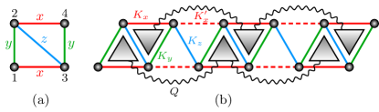
Figure 1: Four-site unit cell and zigzag chain model. (a) The anisotropic chirality pseudospins on the triangular plaquettes are defined according to the bond labels $x$, $y$, and $z$ as written in Eq. (1). (b) In the zigzag chain, spins are coupled by Kitaev interactions. In addition, there is a six-spin interaction that couples the chiralities of triangles with the same orientation (up-pointing or down-pointing) on nearest-neighbor unit cells.

In order to illustrate the spin-chirality duality, we consider a spin model defined on a zigzag chain, given by the Hamiltonian

$$H=H_{K}+H_{Q},$$ (5)

where

$$H_{K}=\sum_{a=x,y,z}K_{a}\sum_{\langle i,j\rangle_{a}}\sigma_{i}^{a}\sigma_{j}^{a}+K_{x}^{\prime}\sum_{\langle i,j\rangle_{x^{\prime}}}\sigma^{x}_{i}\sigma^{x}_{j}$$ (6)

contains the bond-dependent Kitaev interactions. Here $y$ and $z$ bonds couple sites on different legs of the zigzag chain and $x$ bonds lie in the chain direction. We distinguish between two types of $x$ bonds. The bonds with Kitaev coupling $K_{x}$ lie within a unit cell and are represented by solid red lines in Fig. 1(b). The $x$ bonds between sites in neighboring unit cells have coupling $K_{x}^{\prime}$ and are represented by dashed red lines. We focus on the regime of antiferromagnetic Kitaev couplings, $K_{a},K_{x}^{\prime}\geq 0$. The zigzag chain with $K_{x}=K_{x}^{\prime}=K_{y}=K_{z}$ can be viewed as a strip of the Kitaev model on the triangular lattice, whose ground state has been controversial [40, 41, 42, 43]. Besides the Kitaev interactions, we also add terms coupling the chiralities in different unit cells. The six-spin interaction preserves time-reversal symmetry and can be written in terms of the pseudospins in Eq. (1) as

$$H_{Q}=-Q\sum_{r}(\tau^{x}_{1,r}\tau^{x}_{1,r+1}+\tau^{x}_{2,r}\tau^{x}_{2,r+1}),$$ (7)

where $\boldsymbol{\tau}_{1,r}$ and $\boldsymbol{\tau}_{2,r}$ denote the pseudospins for the unit cell at position $r$. This interaction is analogous to the coupling between the scalar spin chiralities on plaquettes of the square lattice proposed in Ref. [2]. Physically, this type of multi-spin interaction can be associated with orbital currents in chiral magnets [58, 59]. We focus on $Q\geq 0$, favoring uniform chirality. The reason for the particular choice of coupling only triangles with the same orientation, see Fig. 1(b), will become clear in Sec. IV.

The relevant symmetries of the model are: time reversal $\mathcal{T}:i\mapsto-i$, $\boldsymbol{\sigma}_{n,r}\mapsto-\boldsymbol{\sigma}_{n,r}$ for $n=1,\dots,4$; a $C_{2}$ rotation symmetry about the center of a $z$ bond $\mathcal{R}:\boldsymbol{\sigma}_{1,r}\leftrightarrow\boldsymbol{\sigma}_{4,-r},\boldsymbol{\sigma}_{2,r}\leftrightarrow\boldsymbol{\sigma}_{3,-r}$; and two discrete spin rotation symmetries $\mathcal{K}_{1}$ and $\mathcal{K}_{2}$ generated by $U_{1}=\prod_{r}\tau^{x}_{1,r}$ and $U_{2}=\prod_{r}\tau^{x}_{2,r}$, respectively, which can be understood as $\pi$ rotations about a different spin axis for each sublattice [60]. Their combined action is known as the Klein symmetry because it is isomorphic to the Klein group, $\mathcal{K}=\mathcal{K}_{1}\times\mathcal{K}_{2}\simeq\mathbb{Z}_{2}\times\mathbb{Z}_{2}$ [39]. The Klein symmetry is found in the Kitaev model on several lattices that obey a certain geometrical condition, including the triangular lattice, but is explicitly broken by more general interactions such as Heisenberg exchange. The product $U_{1}U_{2}=\prod_{r}\prod_{n=1}^{4}\sigma_{n,r}^{z}$ generates the usual global $\pi$ rotation about the $z$ spin axis.

In terms of the pseudospins, the Hamiltonian becomes

$$H = \sum_{r}\bigg{[}\sum_{l=1,2}\left(K_{x}\rho_{l,r}^{z}+K_{x}^{\prime}\rho^{z}_{l,r}\tau^{z}_{l,r}\tau^{z}_{l,r+1}-Q\tau^{x}_{l,r}\tau^{x}_{l,r+1}\right)$$ (8)

$$+K_{y}(\rho_{1,r}^{x}\rho_{2,r}^{x}-\rho_{1,r}^{y}\rho_{2,r}^{y}\tau^{x}_{1,r}\tau^{x}_{2,r})$$

$$+K_{z}(\rho^{x}_{1,r}\rho^{y}_{2,r}\tau^{x}_{2,r}+\rho^{y}_{2,r}\rho^{x}_{1,r+1}\tau^{x}_{1,r+1})\bigg{]}.$$

This Hamiltonian is equivalent to a two-leg ladder with $l=1,2$ playing the role of a leg index. There are two pseudospins 1/2, namely $\boldsymbol{\tau}$ and $\boldsymbol{\rho}$, on each effective site specified by $(l,r)$. In the following sections, we will analyze special limits of the model to establish the existence of a continuous phase transition from a CSS in which $\langle\tau^{x}_{l,r}\rangle\neq 0$ to a magnetic phase in which $\langle\tau^{z}_{l,r}\rangle\neq 0$.

III Chiral Spin State in the exactly solvable model

In this section, we discuss the exact solution of the model with $K_{x}^{\prime}=0$. In this case, the local operators $\tau_{l,r}^{x}$ commute with the Hamiltonian in Eq. (8), generating an extensive number of conserved quantities. For $Q>0$, the ground state has the same eigenvalue for all $\tau_{l,r}^{x}$, corresponding to a uniform spin chirality that spontaneously breaks the $\mathcal{T}$ symmetry and preserves the $C_{2}$ rotation and Klein symmetries. Setting $\tau_{l,r}^{x}=1$, we obtain the effective Hamiltonian for the remaining pseudospins:

$$H_{\rho} = \sum_{r}\bigg{[}K_{x}\sum_{l=1,2}\rho_{l,r}^{z}+K_{y}(\rho_{1,r}^{x}\rho_{2,r}^{x}-\rho_{1,r}^{y}\rho_{2,r}^{y})$$ (9)

$$+K_{z}(\rho^{x}_{1,r}+\rho^{x}_{1,r+1})\rho^{y}_{2,r}-2Q\bigg{]}.$$

The model is now equivalent to a single chain with anisotropic exchange couplings in the $xy$ plane and an effective field in the $z$ direction. We apply the Jordan-Wigner transformation:

$$\rho_{l,r}^{z} = 1-2d^{\dagger}_{l,r}d^{\phantom{\dagger}}_{l,r},$$

$$\rho_{1,r}^{+} = d_{1,r}\prod_{l}\prod_{r^{\prime}<r}(1-2d^{\dagger}_{l,r^{\prime}}d^{\phantom{\dagger}}_{l,r^{\prime}}),$$ (10)

$$\rho_{2,r}^{+} = d_{2,r}(1-2d^{\dagger}_{1,r}d^{\phantom{\dagger}}_{1,r})\prod_{r^{\prime}<r}(1-2d^{\dagger}_{l,r^{\prime}}d^{\phantom{\dagger}}_{l,r^{\prime}}),$$

where $d_{l,r}$ are complex spinless fermions and $\rho^{\pm}_{l,r}=(\rho^{x}_{l,r}\pm i\rho^{y}_{l,r})/2$. The Hamiltonian becomes

$$H_{\rho} = \sum_{r}\bigg{[}-2K_{x}\sum_{l=1,2}d^{\dagger}_{l,r}d^{\phantom{\dagger}}_{l,r}+2K_{y}(d^{\dagger}_{1,r}d^{\dagger}_{2,r}+\text{h.c.})$$ (11)

$$+iK_{z}(d^{\dagger}_{1,r}-d^{\phantom{\dagger}}_{1,r})(d^{\dagger}_{2,r}-d^{\phantom{\dagger}}_{2,r})$$

$$-iK_{z}(d^{\dagger}_{1,r+1}+d^{\phantom{\dagger}}_{1,r+1})(d^{\dagger}_{2,r}+d^{\phantom{\dagger}}_{2,r})\bigg{]}+\text{const}.$$

It is then clear that the model admits an exact solution in terms of free fermions.

The solution for $K_{x}^{\prime}=Q=0$ was discussed in Ref. [13] using a Majorana fermion representation. The key observation is that in this case the zigzag chain reduces to a tricoordinated 1D lattice, called the tetrahedral chain, and the model can be solved by the same methods as Kitaev’s honeycomb model [11]. Using Kitaev’s representation, we write the original spin operator at site $j=(n,r)$ as $\sigma_{j}^{a}=ib^{a}_{j}c^{\phantom{a}}_{j}$, where $b^{a}_{j}$ and $c^{\phantom{a}}_{j}$ are Majorana fermions subjected to the local constraint $b^{x}_{j}b^{y}_{j}b^{z}_{j}c_{j}^{\phantom{x}}=1$. The tetrahedral-chain Hamiltonian can be written as

$$H_{0}=\lim_{K_{x}^{\prime}\to 0}H_{K}=\sum_{a=x,y,z}K_{a}\sum_{\langle j,l\rangle_{a}}iu^{a}_{jl}c_{j}c_{l},$$ (12)

where $u_{jl}^{a}=-ib_{j}^{a}b^{a}_{l}$ are locally conserved $\mathbb{Z}_{2}$ gauge fields defined on the $\langle j,l\rangle_{a}$ bonds, satisfying $u^{a}_{jl}=-u^{a}_{lj}$ and $[u^{a}_{jl},H_{0}]=[u^{a}_{jl},u^{b}_{j^{\prime}l^{\prime}}]=0$. The chirality operators can be identified with the $\mathbb{Z}_{2}$ fluxes in the triangles:

$$\tau^{x}_{1}=u^{x}_{13}u_{32}^{z}u_{21}^{y},\qquad\tau^{x}_{2}=u^{x}_{42}u_{23}^{z}u_{34}^{y}.$$ (13)

Fixing a gauge with $u_{jl}^{a}=\pm 1$ so that $\tau^{x}_{1,r}=\tau^{x}_{2,r}=1$ for all unit cells, we find that the remaining $c$-type Majorana fermions move freely in the background of the static gauge field. Importantly, the spectrum also contains excitations which correspond to changing the $\mathbb{Z}_{2}$ flux configuration. Starting from the state with uniform chirality $\tau^{x}_{l,r}=1$ $\forall l,r$, we refer to an excitation with a single $\tau^{x}_{l,r}=-1$ as a type-$l$ vortex of the $\mathbb{Z}_{2}$ gauge field. In the solvable model, type-1 and type-2 vortices are localized in up-pointing and down-pointing triangles, respectively, and they can be created by changing the sign of a single $u_{jl}^{x}$. Note, however, that physical states must respect a global fermion parity constraint [61].

For $Q=0$, the exactly solvable model suffers from a ground state degeneracy that grows exponentially with system size [13]. The reason is that the energies of the exact eigenstates only depend on the total $\mathbb{Z}_{2}$ flux in each unit cell, i.e., on the product $\tau_{1,r}^{x}\tau_{2,r}^{x}$, rather than the individual chiralities $\tau_{l,r}^{x}$. This degeneracy can be associated with a local symmetry as follows. For $Q=K_{x}^{\prime}=0$, flipping the sign of both chiralities in unit cell $r_{0}$ in Eq. (8) only affects the $K_{z}$ term that couples $d_{1,r_{0}}$ to $d_{2,r_{0}}$ and $d_{2,r_{0}-1}$ in the quadratic Hamiltonian Eq. (11). The sign change can be removed by applying a gauge transformation $d_{1,r_{0}}\mapsto-d_{1,r_{0}}$. Thus, all eigenstates with $\tau_{1,r_{0}}^{x}=\tau_{2,r_{0}}^{x}=-1$ have the same energy as the corresponding eigenstates with $\tau_{1,r_{0}}^{x}=\tau_{2,r_{0}}^{x}=1$. In the Kitaev representation, this means that pairs of vortices located in the same unit cell cost zero energy for $Q=0$. The role of the chirality-chirality coupling that we introduced in Eq. (7) is therefore to impose an energy cost proportional to $Q$ for vortex pairs. For $Q>0$, there are only two ground states with uniform chirality $\tau_{l,r}^{x}=\pm 1$.

Let us now discuss the excitations in the exactly solvable model. First, consider the vortex-free sector with uniform chirality $\tau_{l,r}^{x}=1$. Fixing the set of $u_{jl}^{a}$ in a translationally invariant ansatz and taking a Fourier transform in Eq. (12), we cast the Hamiltonian in the form $H=i\sum_{k>0}C^{\dagger}_{k}\mathcal{A}(k)C^{\phantom{\dagger}}_{k}+\text{const.}$, where $C_{k}^{\dagger}=(c^{\dagger}_{1,k},c^{\dagger}_{2,k},c^{\dagger}_{3,k},c^{\dagger}_{4,k})$ is a four-component spinor in the sublattice basis, with $c^{\dagger}_{n,k}=c^{\phantom{\dagger}}_{n,-k}$, and $\mathcal{A}(k)$ is a matrix obeying $\mathcal{A}^{t}(k)=-\mathcal{A}(-k)$. The dispersion relations of the bands can be calculated analytically for arbitrary values of the Kitaev couplings. The single-fermion energy gap is given by $\Delta_{c}=\sqrt{K_{x}^{2}+K_{y}^{2}+K_{z}^{2}-2K_{z}\sqrt{K_{x}^{2}+K_{y}^{2}}}$ and vanishes for $K_{z}^{2}=K_{x}^{2}+K_{y}^{2}$ [13]. In the fermionic representation, the gap closing involves a change in the $\mathbb{Z}_{2}$ topological invariant $\nu=\text{sgn}\{\text{Pf}[\mathcal{A}(0)]\text{Pf}[\mathcal{A}(\pi)]\}$ for class D in one dimension [62]. The phase for $K_{z}^{2}>K_{x}^{2}+K_{y}^{2}$ corresponds to the nontrivial value $\nu=-1$. However, in the spin representation this transition can be associated with local order parameters. According to the Hamiltonian in Eq. (9), the limit of dominant $K_{z}$ corresponds to the $\boldsymbol{\rho}$ pseudospins ordering in the $xy$ plane. Importantly, nonzero expectation values of $\rho^{x}_{l,r}$ and $\rho^{y}_{l,r}$ break spin-rotation symmetries. Since time-reversal symmetry is already broken by the spontaneous spin chirality, we obtain $\langle\sigma^{z}_{1,r}\rangle\sim\langle\tau^{x}_{1,r}\rangle\langle\rho^{x}_{1,r}\rangle\neq 0$. Thus, for $K_{z}^{2}>K_{x}^{2}+K_{y}^{2}$ we encounter a phase with spontaneous magnetization in the $z$ spin direction coexisting with the spin chirality. Since this phase breaks more symmetries than the pure chiral phase for $K_{z}^{2}<K_{x}^{2}+K_{y}^{2}$, this is a conventional Ising transition and we do not discuss it further. Note that the gap for $c$ fermions closes at the critical point, but vortex excitations remain gapped across this transition.

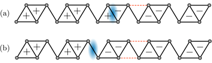
Figure 2: Two types of chirality domain walls. The signs indicate the chirality $\tau_{l,r}^{x}$ for each triangle. (a) In the nonintegrable model with $K_{x}^{\prime}\ll K_{a},Q$, an intracell domain wall can hop one unit cell to the right by applying the $K_{x}^{\prime}$ interaction on the $x^{\prime}$ bond indicated by the dashed line. (b) An intercell domain wall moves two unit cells to the right when the perturbation acts on the two bonds indicated by the dashed lines.

We now turn to vortex excitations. In this case, we compute the energies numerically by diagonalizing the Hamiltonian on a finite chain with open boundary conditions because the localized vortex breaks translational invariance. The energy of a single vortex behaves as $\Delta_{v}=\Delta^{(0)}_{v}+2Q$, where $\Delta^{(0)}_{v}$ denotes the vortex gap for $Q=0$. In particular, for $K_{x}=K_{y}=K_{z}$ we obtain $\Delta^{(0)}_{v}\approx 0.29K_{x}$. The vortex gap vanishes if any of the Kitaev couplings $K_{a}$ approach zero since the broken bonds make the $\mathbb{Z}_{2}$ fluxes ill defined. For $K_{y}=K_{z}\ll K_{x}$, we find $\Delta^{(0)}_{v}\approx K_{y}^{2}/(2K_{x})$.

In the pseudospin representation, it may be more convenient to picture the elementary excitations in the flux sector as domain walls between regions of opposite chiralities. We distinguish between two types of domain walls as illustrated in Fig. 2. We call an intracell domain wall the situation in which the two domains are separated by a unit cell $r_{0}$ with $\tau^{x}_{1,r_{0}}\tau^{x}_{2,r_{0}}=-1$; see Fig. 2(a). By contrast, in an intercell domain wall the chirality switches between two adjacent unit cells so that $\tau^{x}_{1,r}\tau^{x}_{2,r}=1$ for all unit cells in the vicinity of the domain wall; see Fig. 2(b). Starting from a ground state with uniform chirality, we create an intercell domain wall at position $r_{0}$ by applying the string operator $V_{r_{0}}=\prod_{r<r_{0}}\tau_{1,r}^{z}\tau_{2,r}^{z}$, with energy cost $2Q$. An intracell domain wall with energy $\Delta_{v}$ is created by $V_{r_{0}}\tau_{1,r_{0}}^{z}$ or $V_{r_{0}}\tau_{2,r_{0}}^{z}$. A $\mathbb{Z}_{2}$ charge for the domain walls can be defined as the eigenvalue of $\prod_{r}\tau^{x}_{1,r}\tau^{x}_{2,r}=U_{1}U_{2}$; recall that this is the generator of $\pi$ rotations about the $z$ axis. The intracell domain wall is the one which transforms nontrivially under this $\mathbb{Z}_{2}$ symmetry.

The creation of chirality domain walls affects the fermionic spectrum. Here we restrict the parameters to the domain $K_{y}=K_{z}\leq K_{x}$. This condition puts the system in the pure chiral phase with $\nu=1$. We observe numerically that in the presence of an intercell domain wall the fermionic spectrum only comprises a continuum of extended states, as in the vortex-free case. On the other hand, the creation of an intracell domain wall gives rise to a midgap state in which a $c$ fermion is bound near the unit cell with $\tau^{x}_{1,r}\tau^{x}_{2,r}=-1$. The energy of the bound state is not pinned at zero, but varies with the ratio $K_{y}/K_{x}$ as shown in Fig. 3. In particular, the bound state has zero energy for $K_{x}=K_{y}=K_{z}$. We expect the transition from the chiral phase to a non-chiral magnetic phase to be associated with the condensation of domain walls which carry the magnetization degree of freedom in the form of a bound state of a $c$-type matter fermion and a $b$-type flux fermion. This transition will be discussed in the next section.

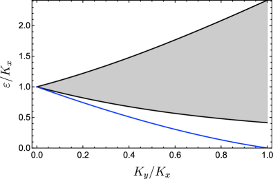
Figure 3: Fermionic spectrum calculated from the Hamiltonian in Eq. (12) for an open chain containing a single intracell domain wall. Here we set $K_{z}=K_{y}$. The shaded region represents the continuum of extended states. The blue line represents the energy of the bound state.

IV Transition to the magnetic state

For $K_{x}^{\prime}>0$, the local chirality operators are no longer conserved because the operator $\tau^{z}_{l,r}\tau^{z}_{l,r+1}$ in Eq. (8) flips the chirality of two triangles with the same orientation in neighboring unit cells. Nevertheless, the parity of the number of type-$l$ vortices, encoded in the eigenvalues of $U_{l}=\prod_{r}\tau^{x}_{l,r}$, are still good quantum numbers. Clearly, the existence of two separately conserved parities is associated with the Klein symmetry. In the regime $K_{x}^{\prime}\ll K_{a},Q$, we can treat the $K_{x}^{\prime}$ term as a perturbation to the solvable model discussed in Sec. III and focus on a subspace with a fixed number of vortices or domain walls. Figure 2 shows the processes that generate an effective hopping amplitude for the domain walls. While the intracell domain wall moves at first order in $K_{x}^{\prime}$, the intercell domain wall only moves at order $(K_{x}^{\prime})^{2}$. As a result, both types acquire a dispersion, but the intracell domain wall has a larger bandwidth. We then expect that, as we increase $K_{x}^{\prime}$ in the regime $Q\gtrsim\Delta_{v}^{(0)}$, the gap for intracell domain walls will eventually close first, driving a phase transition. Below the critical value of $K_{x}^{\prime}$, the mobile domain walls remain gapped and the system is in a CSS characterized by $\langle\tau^{x}_{l,r}\rangle\neq 0$. In the Kitaev representation, the gauge variables $u_{jl}^{y}$ and $u_{jl}^{z}$ still commute with the Hamiltonian, but $u_{jl}^{x}$ become fluctuating, and the chiral phase corresponds to $\langle u_{jl}^{x}\rangle\neq 0$.

To examine the phase transition, let us consider the limit of highly anisotropic Kitaev interactions. For $K_{y},K_{z}\to 0$, the $\boldsymbol{\rho}$ pseudospins are fully polarized with $\rho^{z}_{l,r}=-1$ in the ground state. This condition imposes strong antiferromagnetic correlations in the $x$ spin direction between two spins on the same leg and in the same unit cell; see Eqs. (3) and (4). In the regime $K_{y},K_{z}\ll K_{x}$, we can safely assume that the $\boldsymbol{\rho}$ pseudospins are gapped out. We derive an effective Hamiltonian in the low-energy subspace by applying perturbation theory to second order in $K_{y}$ and $K_{z}$. We obtain

$$H_{\rm eff} = -\sum_{r}\sum_{l=1,2}\left(K_{x}^{\prime}\tau^{z}_{l,r}\tau^{z}_{l,r+1}+Q\tau^{x}_{l,r}\tau^{x}_{l,r+1}\right)$$ (14)

$$-K_{\perp}\sum_{r}\tau^{x}_{1,r}\tau^{x}_{2,r}+\text{const.},$$

where $K_{\perp}\approx K_{y}^{2}/(2K_{x})$. This Hamiltonian describes a two-leg ladder with weakly coupled XY chains. Note that the interchain coupling only involves the $x$ components of the pseudospins. The interactions $\tau^{a}_{1,r}\tau^{a}_{2,r}$ with $a=y,z$ are forbidden by the Klein symmetry.

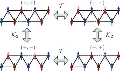
Figure 4: Four ground states in the magnetic phase. The up and down arrows represent the magnetization in the $x$ spin direction. The symmetries that connect the different states are also indicated.

This analysis reveals that the model with $K_{y}=K_{z}=0$ and $K_{x},K_{x}^{\prime},Q>0$ is also exactly solvable. Setting $K_{\perp}=0$, we see that the Hamiltonian reduces to two identical and decoupled XY chains, even though spins on different legs of the original zigzag chain are coupled by the six-spin interaction. The exact excitation spectrum can be calculated by performing a Jordan-Wigner transformation. The critical point occurs at $K_{x}^{\prime}=Q$. The chirality vanishes continuously as we approach the critical point from $K_{x}^{\prime}<Q$. For $K_{x}^{\prime}>Q$, the system enters another ordered phase characterized by $\langle\tau^{z}_{l,r}\rangle\neq 0$. Since $\rho_{l,r}^{z}=-1$, this implies $\langle\sigma^{x}_{1,r}\rangle=-\langle\sigma^{x}_{3,r}\rangle\neq 0$ and $\langle\sigma^{x}_{2,r}\rangle=-\langle\sigma^{x}_{4,r}\rangle\neq 0$. Thus, we find a collinear magnetic phase with spontaneous magnetization in the $x$ spin direction. There are four ground states, labeled by $(\text{sgn}\langle\sigma^{x}_{1,r}\rangle,\text{sgn}\langle\sigma^{x}_{2,r}\rangle)$ and represented in Fig. 4. The magnetic order in the zigzag chain is analogous to the stripe phase of the antiferromagnetic Kitaev model on the triangular lattice as obtained in Ref. [43]. The pair of states $(+,+)$ and $(-,-)$ are conjugated by $\mathcal{T}$ symmetry, and likewise for the pair $(+,-)$ and $(-,+)$. The $(+,+)$ and $(-,-)$ states break the $\mathcal{R}$ spatial rotation symmetry, but preserve $\mathcal{R}\mathcal{T}$. The degeneracy between $(+,+)$ and $(+,-)$ is protected by the $\mathcal{K}_{2}$ symmetry; both $\mathcal{K}_{1}$ and $\mathcal{K}_{2}$ are spontaneously broken in this phase. All four ground states are invariant under the combination of time reversal and global $\pi$ rotation about the $z$ spin axis, a symmetry broken in the CSS. Remarkably, the $\mathcal{T}$ symmetry is broken on both sides of the transition, but restored at criticality. In the magnetic phase, the elementary excitations are kinks or domain wall in the staggered magnetization. The magnetization domain walls are mobile for any $Q>0$ and condense when we approach the phase transition from $K_{x}^{\prime}>Q$.

We determine the universality class of the transition by taking the continuum limit in the effective Hamiltonian. Starting from $K_{\perp}=0$, we bosonize the pseudospins in the XY chains following the standard procedure [63] and then add the interchain coupling $K_{\perp}$ as a perturbation. We obtain the Hamiltonian density

$$\mathcal{H}_{\rm bos} = \sum_{l}\left[\frac{v\kappa}{2}(\partial_{x}\theta_{l})^{2}+\frac{v}{2\kappa}(\partial_{x}\phi_{l})^{2}+\lambda\cos(\sqrt{4\pi}\theta_{l})\right]$$ (15)

$$-\lambda_{\perp}\cos(\sqrt{\pi}\theta_{1})\cos(\sqrt{\pi}\theta_{2}),$$

where the bosonic fields satisfy $[\phi_{l}(x),\partial_{x^{\prime}}\theta_{l^{\prime}}(x^{\prime})]=i\delta_{ll^{\prime}}\delta{(x-x^{\prime})}$, $v$ is the velocity of the pseudospin excitations, $\kappa$ is the Luttinger parameter, and $\lambda,\lambda_{\perp}>0$ are the coupling constants of the relevant operators with scaling dimensions $1/\kappa$ and $1/(2\kappa)$, respectively. In the vicinity of the transition, we have $v\sim K_{x}^{\prime}$, $\lambda\sim K_{x}^{\prime}-Q$, $\lambda_{\perp}\sim K_{\perp}$, and $|\kappa-1|\sim(K_{\perp}/K_{x}^{\prime})^{2}$. The bosonized pseudospin operators can be written as $\tau^{x}_{l,r}\sim\cos(\sqrt{\pi}\theta_{l})$ and $\tau^{z}_{l,r}\sim\sin(\sqrt{\pi}\theta_{l})$.

For $\lambda_{\perp}=0$, the bosonic Hamiltonian reduces to two decoupled sine-Gordon models. The critical point at $\lambda=0$ contains two massless bosons and is described by a CFT with central charge $c=2$. The continuous symmetry $\theta_{l}\mapsto\theta_{l}+\text{const.}$ of the effective field theory at the critical point can be traced back to the lattice model. For $K_{y}=K_{z}=0$ and $Q=K_{x}^{\prime}>0$, the operators $Y_{l}=\sum_{r}\tau^{y}_{l,r}$ with $l=1,2$ become conserved charges in the sector with $\rho^{z}_{l,r}=-1$. Away from the critical point, the relevant cosine perturbation flows to strong coupling under the renormalization group. The chiral phase corresponds to $\lambda<0$, with $\lambda\to-\infty$ at low energies pinning the $\theta$ field at $\theta_{l}=0$ or $\theta_{l}=\sqrt{\pi}$. For $\lambda>0$, the flow to $\lambda\to\infty$ pins the bosonic fields at $\theta_{l}=\sqrt{\pi}/2$ or $\theta_{l}=3\sqrt{\pi}/2$, corresponding to the magnetic phase. For $\lambda_{\perp}=0$, both phases have a fourfold degenerate ground state. The extra ground state degeneracy of the chiral phase is due to the decoupling of the chiralities with different $l$ for $K_{\perp}=0$ in Eq. (14).

When we switch on $\lambda_{\perp}>0$, the bosonic fields on different legs are coupled by a strongly relevant operator. According to the $c$ theorem [64], the central charge of the CFT must decrease. Since the cosine operators commute with each other, we can proceed with a semiclassical analysis of the effective potential $V(\theta_{1},\theta_{2})=\lambda\sum_{l}\cos(\sqrt{4\pi}\theta_{l})-\lambda_{\perp}\cos(\sqrt{\pi}\theta_{1})\cos(\sqrt{\pi}\theta_{2})$. For $\lambda_{\perp}>0$, the potential only becomes flat in the directions $\theta_{2}=\pm\theta_{1}$ (mod $2\sqrt{\pi}$) of the $(\theta_{1},\theta_{2})$ plane when $\lambda=\lambda_{\perp}/4>0$, as opposed to a completely flat potential when $\lambda=\lambda_{\perp}=0$. This means that the interchain coupling leaves out only one gapless boson at the transition, either $\theta_{+}=(\theta_{1}+\theta_{2})/\sqrt{2}$ or $\theta_{-}=(\theta_{1}-\theta_{2})/\sqrt{2}$. As a consequence, the generic transition for $\lambda_{\perp}>0$ has central charge $c=1$, associated with a single emergent U(1) symmetry. This result is similar to the Néel-VBS transition in frustrated spin chains [32, 33]. At criticality, the correlation functions for both order parameters decay as power laws with the same exponent. Note that the transition at a critical value of $\lambda>0$ enlarges the region occupied by the chiral phase in comparison with the result for $\lambda_{\perp}=0$.

We can understand the ground state degeneracy by pinning the bosonic fields in the presence of the $\lambda_{\perp}$ interaction. Assuming that $\lambda_{\perp}$ gaps out $\theta_{-}$, we fix $\theta_{2}=\theta_{1}$. In the chiral phase, this condition implies $\theta_{1}=\theta_{2}=0,\sqrt{\pi}$; the two choices correspond to the ground states with either sign of $\langle\tau^{x}_{1,r}\rangle=\langle\tau^{x}_{2,r}\rangle\neq 0$. If we assume instead that $\lambda_{\perp}$ gaps out $\theta_{+}$ and fix $\theta_{2}=-\theta_{1}$, we find precisely the same expectation values for the local physical operators. Thus, the ground state of the chiral phase is twofold degenerate for $\lambda_{\perp}>0$. On the other hand, the choice of gapping out $\theta_{+}$ or $\theta_{-}$ affects the expectation value of the magnetization when we pin the bosonic fields at $\theta_{1}=\pm\theta_{2}=\sqrt{\pi}/2,3\sqrt{\pi}/2$. In this case, there are still four possibilities labeled by the signs of $\langle\tau^{z}_{1,r}\rangle$ and $\langle\tau^{z}_{2,r}\rangle$. Provided that the Hamiltonian preserves the Klein symmetry, the ground state of the magnetic phase remains fourfold degenerate. In fact, the effective field theory allows us to analyze the effects of breaking the Klein symmetry, which in the bosonic representation acts as $\mathcal{K}_{l}:\phi_{l}\mapsto-\phi_{l},\theta_{l}\mapsto-\theta_{l}$. Adding the perturbation $\lambda_{\perp}^{\prime}\sin(\sqrt{\pi}\theta_{1})\sin(\sqrt{\pi}\theta_{2})$ to the Hamiltonian density in Eq. (15), we find that the total potential still pins $\theta_{2}=\pm\theta_{1}$ and leaves out one gapless boson with $c=1$ at the transition. However, the ground state degeneracy of the magnetic phase is reduced to twofold, as the new interaction selects either $(+,+)$ and $(-,-)$ or $(+,-)$ and $(-,+)$, depending on the sign of $\lambda_{\perp}^{\prime}$.

In the bosonic Hamiltonian Eq. (15), we dropped the symmetry-allowed cosine operators such as $\cos(\sqrt{16\pi}\phi_{l})$ because they are highly irrelevant for $\kappa\approx 1$. Vertex operators of the form $\exp(im\sqrt{\pi}\phi_{l})$ with $m\in\mathbb{Z}$ create or annihilate domain walls, which in the bosonic theory correspond to kinks and antikinks in the field configuration, $\theta_{l}(x\to\infty)-\theta_{l}(x\to-\infty)=\pm\sqrt{\pi}$. In a semiclassical picture for the chiral phase, to go from the ground state with $\theta_{l}=0$ to $\theta_{l}=\pm\sqrt{\pi}$, the bosonic fields have to go through $\theta_{l}=\pm\sqrt{\pi}/2$, which can be interpreted as the magnetization $\langle\tau^{z}_{l,r}\rangle\sim\langle\sin(\sqrt{\pi}\theta_{l})\rangle$ residing at the topological defect of the CSS. The same argument can be used to see how domain walls in the magnetic phase must carry spin chirality. Near the transition, the processes that change the number of domain walls in either picture become irrelevant.

Similar phenomenology is generally found in effective field theories for DQC [21, 22, 23, 24]: topological defects in one phase nucleate the order parameter of the other phase. If the order parameters are written in terms of fractionalized excitations, the resulting constraints lead to an emergent gauge field on which the topological defects are charged. One can then understand both phases as distinct confined regimes, merging in a critical region corresponds to a gapless phase in the gauge theory.

In our model, the domain wall description can be obtained by a refermionization of the bosonic fields, defining the chiral fermions $\psi_{R/L,l}\sim\exp\left[-i\sqrt{\pi}(2\phi_{l}\mp\theta_{l}/2)\right]$. The physical spin operators are then given by fermion bilinears. In terms of the two-component spinors $\Psi^{\dagger}_{l}=(\psi^{\dagger}_{L,l},\psi^{\dagger}_{R,l})$, we have $\tau^{x}_{l,r}\sim\Psi^{\dagger}_{l}\sigma^{x}\Psi^{\phantom{\dagger}}_{l}$ and $\tau^{z}_{l,r}\sim\Psi^{\dagger}_{l}\sigma^{y}\Psi^{\phantom{\dagger}}_{l}$, with $\sigma^{a}$ the Pauli matrices acting in the internal space. The effective Hamiltonian includes density-density interactions which arise from the cosine operators as well as quadratic terms in Eq. (15). The emergent symmetry at the critical point is manifested as Noether charges of the fermions, preventing pairing terms from appearing in the Hamiltonian. A mean-field decoupling of the quartic interactions generates mass terms for the chiral fermions in the ordered phases. Solitonic configurations in the mass terms support fermion bound states via the Jackiw-Rebbi mechanism [65], confirming the previous interpretation in terms of domain walls. Note that this mechanism applies to smooth domain walls in the low-energy theory for the transition, as opposed to the sharp domain walls deep in the chiral phase discussed in Sec. III. For a smooth domain wall, a zero-energy bound state is formed even if the phase is topologically trivial [66].

To describe the transition in the fermionic picture, we start from the assumption of an emergent U(1)$\times$U(1) symmetry, which can then be gauged. The coupling to a U(1) gauge field can be obtained by noticing that the representation of the physical operators has a gauge redundancy, $\Psi_{l}(x)\mapsto e^{ie_{l}\Lambda_{l}(x)}\Psi_{l}(x)$, where $e_{l}$ play the role of gauge charges. We then impose a constraint on the fermion densities $\Psi^{\dagger}_{l}\Psi^{\phantom{\dagger}}_{l}\sim\partial_{x}\theta_{l}$, as usual in parton constructions [67]. The resulting gauge-invariant lagrangian has the form

$$\mathcal{L}=\sum_{l=1,2}\bar{\Psi}_{l}i\gamma^{\mu}(\partial_{\mu}-ie_{l}a_{\mu})\Psi_{l}+\frac{1}{4g^{2}}(f_{\mu\nu})^{2}+\cdots,$$ (16)

where we introduced the Maxwell tensor $f_{\mu\nu}=\partial_{\mu}a_{\nu}-\partial_{\nu}a_{\mu}$, the parameter $g$ in the Maxwell term controls the fluctuations of the gauge field, and we omitted quartic terms associated with short-range interactions. The terms highlighted in Eq. (16) comprise the $N_{f}=2$ Schwinger model in $1+1$ dimensions, known to reduce to a single massless boson at low energies [68, 69, 70]. The gauge charges can be chosen arbitrarily as $e_{l}=\pm 1$. The relative sign between $e_{1}$ and $e_{2}$ selects symmetric or antisymmetric modes with respect to exchanging the leg index, and is analogous to pinning either $\theta_{+}$ or $\theta_{-}$ in the bosonic theory. The critical point corresponds to fine tuning the quartic interactions so that the bosonic mode remains gapless, as described by Eq. (15) after we fix $\theta_{2}=\pm\theta_{1}$. Once again, we come to the conclusion that the transition between the chiral and magnetic phases is described by a $c=1$ CFT. At the fixed point, the two chiral sectors of the gapless boson decouple, and the CFT has an enlarged U(1)$\times$U(1) symmetry [71].

V Numerical Results

In this section, we present our DMRG results for the phase transition between the CSS and the collinear magnetic state. To investigate the phases and the nature of the phase transition, we consider the zigzag chain with six-spin interactions described by the Hamiltonian in Eq. (5), equivalent to Eq. (8), and the two-leg XY ladder defined in Eq. (14). In particular, we show results for the expectation values $\langle\tau^{x,z}_{l,r}\rangle$, the susceptibility of the ground-state energy density, and the entanglement entropy (EE).

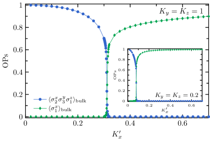
Figure 5: Anisotropic spin chirality and local magnetization for the zigzag chain model, see Eqs. (5)-(7), as a function of $K_{x}^{\prime}$ for $K_{x}=Q=1$ and $K_{y}=K_{z}=1$. The inset shows the same order parameters for $K_{y}=K_{z}=0.2$.

To compute the physical properties of interest, we have considered open chains with a maximum length of $L=400$. Keeping up to 400 states to represent the truncated DMRG blocks, we find that the largest truncation error acquired is smaller than $10^{-9}$ at the final sweep. As discussed in Secs. III and IV, both chiral and magnetic phases exhibit degenerate ground states. Thus, to avoid linear combinations of the ground states in the numerical simulations, we have included weak and suitable perturbations that couple to the order parameters at the chain edges and select one ground state for a given phase. These small local perturbations do not affect the bulk properties, probed by observables computed near the middle of the chain.

Let us first focus on the zigzag chain model with six-spin interactions given by Eq. (5). In Fig. 5, we show the bulk values for the chiral and magnetic order parameters as a function of $K^{\prime}_{x}$ for $K_{a}=Q=1$, with $a=x,y,z$. While the CSS is characterized by a finite anisotropic spin chirality, the magnetically ordered phase displays an antiferromagnetic alignment along the $x$ spin direction (see Fig. 4). Note that there is a single phase transition at a critical value of $K_{x}^{\prime}$. We have also considered the regime $K_{y}=K_{z}<K_{x}$ and found that the chiral phase becomes narrower as we decrease the ratio $K_{y}/K_{x}$, but the behavior is qualitatively the same as for $K_{x}=K_{y}=K_{z}$. No other transitions are observed as we vary $K_{y}/K_{x}$ for fixed $Q=K_{x}$; see the inset in Fig. 5.

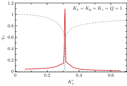
Figure 6: Susceptibility of the ground-state energy density as a function of $K_{x}^{\prime}$ for $K_{x}=K_{y}=K_{z}=Q=1$. The dashed lines represent the order parameters shown in the main plot of Fig. 5. The divergent behavior of $\chi_{e}$ at $K^{\prime}_{x}\approx 0.312$ determines the critical point.

To pinpoint the location of the phase transition, we have analyzed the energy susceptibility, defined as

$$\chi_{e}=-\frac{\partial^{2}e_{0}}{\partial K_{x}^{\prime 2}},$$ (17)

where $e_{0}$ is the ground-state energy per site. In $d$ dimensions, the energy susceptibility diverges at the critical point as a power law with exponent $\alpha=(2/\nu)-(d+z)$, where $\nu$ and $z$ are the correlation and the dynamical critical exponents [72, 49]. In Fig. 6, we show $\chi_{e}$ as a function of $K_{x}^{\prime}$ for $K_{a}=Q=1$. Note that $\chi_{e}$ exhibits a prominent peak, whose position in the $K_{x}^{\prime}$ domain determines the critical point $K_{x}^{\prime}=K^{\prime}_{x,\text{crit}}$. For the set of couplings shown in Fig. 6, we obtain $K^{\prime}_{x,\text{crit}}\approx 0.312$. To verify the accuracy of the critical points extracted from $\chi_{e}$, we have also estimated $K^{\prime}_{x,\text{crit}}$ from the analysis of the inflection point of the order parameters and the highest Schmidt eigenvalue. The latter was proposed in Ref. [49] as a sensitive measure to detect phase transitions. Altogether, we found excellent agreement among the estimates obtained from these distinct procedures.

We now turn to the effective Hamiltonian in Eq. (14), valid in the regime $K_{y},K_{z}\ll K_{x}$. This model describes two weakly coupled XY chains with interchain coupling along the $x$ direction. In comparison with the original zigzag chain in Eq. (5), the dimension of the local Hilbert space in the effective ladder model is reduced by a factor of 2, providing a significant advantage for numerical simulations. Since we observed the same qualitative behavior for the original model with $K_{x}=K_{y}=K_{z}$ as for small $K_{y,z}/K_{x}$, see Fig. 5, we expect the effective XY ladder model in Eq. (14) to capture the essential characteristics of the phase transition. Carrying out the same analysis as for the zigzag chain, we again find only one transition for fixed $Q$ and different values of $K_{x}^{\prime}$. In agreement with the analysis in Sec. IV, the transition for $K_{\perp}>0$ shifts to larger values of $K_{x}^{\prime}$ as compared to $K_{x}^{\prime}=Q$ in the exactly solvable case $K_{\perp}=0$. Setting $Q=1$, we determined the critical point $K_{\perp}=K_{\perp,\text{crit}}$ for $K_{x}^{\prime}=1.2$ and $1.4$. The acquired values are $K_{\perp,\text{crit}}\approx 0.187$ and $0.49$, respectively.

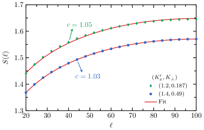
Figure 7: Entanglement entropy as a function of partition size $\ell$ for the critical two-leg XY ladder model, see Eq. (14), with $(K_{x}^{\prime},K_{\perp})=(1.2,0.187)$ and $(1.4,0.49)$. The symbols represent the DMRG results for chain length $L=200$ and open boundary conditions. The solid red lines are fits to our numerical data using Eq. (18). The estimates for the central charge are indicated in the plot.

We investigate the universality class of the transition by extracting the central charge from the EE. Consider a chain composed of two partitions $\mathcal{A}$ and $\mathcal{B}$ with $\ell$ and $L-\ell$ sites, respectively. The EE is then defined as $S(\ell)=-\mathrm{Tr}(\rho_{\mathcal{A}}\ln\rho_{\mathcal{A}})$, where $\rho_{\mathcal{A}}$ is the reduced density matrix of partition $\mathcal{A}$. For critical 1D systems, the asymptotic behavior of $S(\ell)$ predicted from CFT is given by [73]

$$S(\ell)=\frac{c}{3\eta}\ln\left[\frac{L}{\pi}\sin\left(\frac{\pi}{L}\ell\right)\right]+b,$$ (18)

where $c$ is the central charge, $b$ is a nonuniversal constant, and $\eta=1(2)$ for periodic (open) chains. In Fig. 7, we show the EE as a function of $\ell$ for $(K_{x}^{\prime},K_{\perp,\text{crit}})=(1.2,0.187)$ and $(1.4,0.49)$. We consider values of $\ell$ corresponding to partitions with an even number of rungs in an open chain. Fitting our DMRG results using Eq. (18), we obtain $c\approx 1.05$ and $1.03$, respectively. Considering different fitting intervals and system sizes, we have checked that our estimates are robust and the maximum deviation from $c=1$ is about $9\%$. The logarithmic scaling of the entanglement entropy with the subsystem size is clear evidence of critical behavior at the transition. Moreover, our results show remarkable agreement with the central charge predicted in Sec. IV. Finally, we have also investigated the effects of an explicit Klein-symmetry breaking by adding the interaction $K_{\perp}^{\prime}\sum_{r}\tau^{z}_{r,1}\tau^{z}_{r,2}$ to the Hamiltonian in Eq. (14). While the values of the critical couplings shift with the perturbation, no further transitions are observed and the central charge remains the same. Therefore, the Klein symmetry does not affect the universality class of the transition.

VI Future directions in 2D

The local pseudospin mapping of Eqs. (1)-(4) can be used to fabricate Hamiltonians with six-spin interactions that reduce to known spin-1/2 models in two dimensions once we freeze out the $\boldsymbol{\rho}$ pseudospins. The phase with long-range order in $\tau^{x}$ would then correspond to a CSS. However, it is unclear if this approach can lead to deconfined transitions between chiral and magnetic phases in 2D compass models. The existence of a robust continuous transition between competing ordered phases is conjectured to be connected to non-trivial symmetry properties of topological defects [21, 22, 23, 24]. Therefore, if the $\boldsymbol{\tau}$ pseudospin is defined envisioning the defects of $\tau^{x}$ and $\tau^{z}$ ordered phases on a given lattice, it may be possible to engineer a spin Hamiltonian in which gapping out the $\boldsymbol{\rho}$ pseudospin results in an effective model with a deconfined transition. An effective field theory description would then be described by a parton decomposition consistent with the defects [24, 32].

A more interesting question is whether a continuous phase transition from a CSS to a collinear magnetic state or another ordered phase can be found in models that do not require six-spin interactions. Like the solvable model discussed in Sec. III, the Yao-Kivelson model on the star lattice [12] exhibits spontaneous time-reversal-symmetry breaking and two chiral phases separated by a phase transition at which the gap for dynamical matter fermions closes. In this case, the phases are topologically trivial and nontrivial chiral spin liquids distinguished by the Chern number. In the exact solution using the Kitaev representation, the topological excitations are vortices of the emergent $\mathbb{Z}_{2}$ gauge field, which bind Majorana zero modes in the nontrivial phase. One may then wonder if closing the vortex gap by adding integrability-breaking perturbations to the Yao-Kivelson model could drive an unconventional transition to a magnetic phase. In a parallel development, the dynamics of $\mathbb{Z}_{2}$ flux excitations and the relation to phase transitions in the extended Kitaev honeycomb model at zero magnetic field has been discussed based on parton mean-field theories [74, 75] and a variational approach [76].

Moving on to SU(2)-invariant models, the situation becomes less clear. Here new dualities involving the scalar spin chirality [55] may prove instrumental. Numerically, a chiral spin liquid with spontaneous time-reversal-symmetry breaking has been found in the extended Heisenberg model on the kagome lattice [7, 8]. DMRG results on cylinder geometries suggest that the quantum phase transition from the chiral spin liquid to the $q=(0,0)$ Néel state is at least not strongly first order [8]. The same can be said about transitions out of the chiral spin liquid phase in the triangular lattice Hubbard model [77].

VII Conclusions

In this work, we introduced a Kitaev-type model defined on the zigzag chain and showed the presence of two phases separated by a transition. On one side, we have a chiral spin state stabilized by coupling three-spin chiralities. On the other side, there is a collinear magnetic state also found in the natural extension of our model to two dimensions, the Kitaev model on the triangular lattice [43]. Numerical analysis and field theory arguments indicate a continuous phase transition, which would be forbidden by the traditional LGW paradigm due to the competing nature of the order parameters. Furthermore, a low-energy parton construction suggests an emergent symmetry along with the condensation of topological defects (domain walls) in the transition, similar to the phenomenology found in deconfined quantum criticality in two dimensions. Our work then provides an example of the recently found deconfined transitions in one dimension [33, 32, 36].

Further numerical investigation of this transition is also warranted. Critical exponents in correlation functions vary continuously for a $c=1$ (Gaussian) transition, and it would be interesting to see this behavior as one tunes the microscopic parameters. Moreover, our model may host other phases and transitions for a different range of parameters. We leave the complete mapping of the ground state phase diagram and the study of correlation functions at criticality for future work.