Churn modeling of life insurance policies via statistical and machine learning methods - Analysis of important features

Abstract

Life assurance companies typically possess a wealth of data covering multiple systems and databases. These data are often used for analyzing the past and for describing the present. Taking account of the past, the future is mostly forecasted by traditional statistical methods. So far, only a few attempts were undertaken to perform estimations by means of machine learning approaches. In this work, the individual contract cancellation behavior of customers within two partial stocks is modeled by the aid of various classification methods. Partial stocks of private pension and endowment policy are considered. We describe the data used for the modeling, their structured and in which way they are cleansed. The utilized models are calibrated on the basis of an extensive tuning process, then graphically evaluated regarding their goodness-of-fit and with the help of a variable relevance concept, we investigate which features notably affect the individual contract cancellation behavior.

Statements relating to the ethics and integrity policies:
 

Unfortunately, our data are confidential and not available. However, if requested by the referees, we could make example code available, which illustrates the usage of our fitting procedures. Furthermore, we have no funding and no conflict of interest to declare.

Keywords: Classification problems, Big Data, Life Insurance, Churn prediction, Variable Relevance

1 Introduction

Data are among the biggest treasures of the 21st century. Financial service providers like insurers hold large data quantities which could provide a significant improvement of the comprehension of their business if exploited correctly. Life insurance as one of the most important and oldest sectors of insurance is characterized by its long-term contracts. Inventory management turns out to be a very central aspect for better understanding and controlling the existing contracts in the company. An important goal is the creation of short- and long-term strategies, including the evaluation of solvency, as it is frequently examined by various surveillance authorities. One sub-aspect of the inventory management is the contract reversal. Being able to comprehend this aspect and its causes can lead to various actions like the reversal prevention.

Due to the rapid development of inventory management systems and the increase of computational power, many applications of Big Data became more and more relevant in recent years. Along with this, powerful and advanced methods of statistical and machine learning have been developed, which allow to analyze large data quantities, to recognize connections within the data and to predict future events. Lately, machine learning techniques have become more and more important in the context of modeling insurance data, see e.g. Makariou et al. (2021); Devriendt et al. (2021); Denuit et al. (2021); Gan (2013). In this work, some of these methods shall be used for a better understanding of the individual contract cancellation behavior of a large German life insurer’s clients. For this purpose, classical statistical approaches like the logit regression model (Fahrmeir and Tutz, 2001; McCullagh and Nelder, 2019) and the elastic net regularization method (Zou and Hastie, 2005) as well as modern machine learning methods are employed. From the field of machine learning, several tree-based approaches are considered. These include Classification and Regression Trees (CART; Breiman et al., 1984), Random Forest (Breiman, 2001) and XGBoost (Chen and Guestrin, 2016).

In this manuscript, first we will briefly introduce the previous methods for statistical modeling as well as various evaluation approaches for the models. These are then applied to the partial stocks of endowment life insurance (ELI) and of private pension insurance. For each approach the respective best model regarding the so-called Area Under the Curve (AUC; see, e.g., Bradley, 1997) is determined by means of parameter tuning. Subsequently, the resulting models are investigated with respect to the relevant factors for decision making. These factors shall give information on the relationship between the contract reversal and various contract parameters and individual client information.

In Section 2, we briefly describe the underlying research problem and motivate why it is useful to understand individual contract termination behavior in more detail. Section 3 includes a description of the database used for model building. We describe the general structure of the data as well as key aspects of data preprocessing. Then, in Section 4, we briefly describe the different approaches used for model building, their main aspects, and how these models are evaluated. Specifically, in Section 4.4, we describe in detail a certain measure of Varibale Relevance defined in this work. Next, we present the main results in Section 5, comparing the different approaches and their corresponding tuned models using the methods described in Section  4. Finally, we summarize the results in Section 6 and give an outlook on how this work can be extended.

2 Motivation

Life insurance differs from other types of insurance in that it offers products with a very long term. Particularly, in term risk life insurance, endowment life insurance and occupational disability insurance, high premiums are paid in the beginning for acquisition costs and administrative expenses. Over time, the initial costs incurred are compensated by the premiums and the associated investment income. Subsequent to this period, profits are generated.

In order to create a stable financial basis in the long term, it is necessary to address individual contract cancellation behavior. Although this subject is well researched in the deterministic field of actuarial science, to the best of our knowledge, there are few analyses that use statistical techniques to predict future lapse-related charges. Indeed, it is of great advantage for an insurance company to be able to anticipate certain lapse rates, because then suitable measures could be taken to prevent lapses.

This manuscript deals with a number of statistical and machine learning estimation methods which attempt to investigate the lapse behavior of individual contracts of the portfolio of a large German life insurer on a large data basis, and to compare them with respect to their predictive validity. All calculation have been performed in the statistical software program R Core Team (2020).

3 Data

In order to build up the estimation methods for explanation and prediction of the cancellation behavior of individual contracts, a sufficiently large and high-quality data base is required. In the context of this work, we were able to access a large amount of information from the data warehouse (DWH). It contains an extensive collection of information on insurance contracts and insured persons, which in turn is grouped according to various logics.

Initial considerations about which information is relevant for investigating lapse behavior in individual contracts led to the conclusion that the most suitable data basis is portfolio data on the basis of contract information. This means that, in addition to information on the main insurance policy, information on all associated supplementary insurance policies is also available. The period 1/1/2018-12/31/2018 was selected as the study period.

Each insurance contract is assigned an anonymous contract number within the DWH. The contract part ID can then be used to assign the corresponding contract part. Hence, a contract part of an insurance can be uniquely assigned by the combination of both characteristics within the DWH. An example of this structure is displayed in Table 1. Since these two pieces of information are unique, but also randomly filled, they are only important during data preparation and are neglected for model building.

contract ID	contract part ID	$\ldots$	sum insured	actuarial interest rate
1678655	1	$\cdots$	48.250	3,25
1678655	2	$\cdots$	37.630	2,75
4789889	1	$\cdots$	18.470	1,25
4912002	1	$\cdots$	16.800	1,25
5100200	1	$\cdots$	4.520	0,9
$\vdots$	$\vdots$	$\vdots$	$\vdots$	$\vdots$

Table 1: Structure of the inventory data. In this example, four contracts are shown, as indicated by the contract number. The first contract contains two contract parts, the others only the main insurance. The contract parts contain, among other things, the information on the sum insured and the actuarial interest rate.

Moreover, for an analysis of the cancellation behavior of individual customers, statistical information on the annual premium, the sum insured, and the actuarial interest rate associated with the contract, which among other things enables the contract to be classified on the time axis, can also be expected to be of great importance.

Another important data source is collection data. The prior events listed there can be classified into eight categories on the basis of one feature that describes the type of collection process, such as, e.g., delay of premium payments and/or resulting dunning procedures. For each insurance contract and each of these eight categories, the number of prior events within the last five years (for endowment insurance) or within the last year (for private pension insurance) is then calculated. The distinction between these two types of insurance could be made on the basis of the name of the contract part.

Besides the acquisition of the data, their preprocessing was an essential part of the preparatory work, which had to be carried out in advance of our analyses. The preprocessing is divided into some central steps, which are described in the following.

3.1 Feature Engineering

One of the most important features that had to be created is the binary target variable “individual contract cancellation”. Here, the reason for the contract’s termination was considered: If it was a canceled contract, the variable was assigned the value 1; if the contract had another or no reason for termination, the variable was assigned the value 0. Since it is common for life insurance products to have a rather long duration, only very few contracts in the respective final data set have the value 1 in the target variable “individual contract cancellation”, see Figure 1 and Table 2. Hence, the data set is “unbalanced” with respect to the target variable. We shall describe in the following how this can be handled.

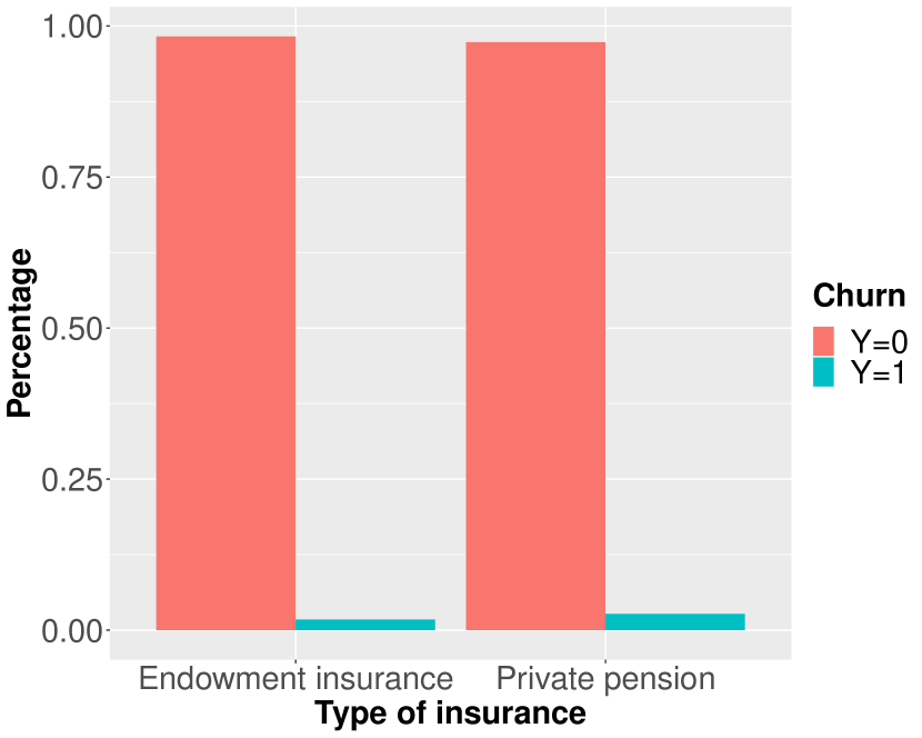
Figure 1: Proportions of canceled and non-cancelled contracts within the data sets under review.

	contract ID	contract part ID	$\ldots$	contract beginn	occupation	$\ldots$	contract cancelled?
1:	1678655	1	$\cdots$	01.02.2001	Baker	$\cdots$	1
2:	1678655	2	$\cdots$	01.04.2005	Baker	$\cdots$	0
3:	4789889	1	$\cdots$	01.07.2015	Police Officer	$\cdots$	0
4:	4912002	1	$\cdots$	01.09.2015	Craftsman	$\cdots$	0
5:	5100200	1	$\cdots$	01.03.2017	Actuary	$\cdots$	0
$\vdots$	$\vdots$	$\vdots$	$\vdots$	$\vdots$	$\vdots$	$\vdots$	$\vdots$

Table 2: Extension of the inventory data with self-built features. The contracts from Figure 1 are extended by, among others, the contract start date, the categorized occupation and the target variable individual contract cancellation.

From the temporal information regarding the beginning and expiration of the insurance, the information of the total, already passed and remaining contract duration was calculated and added to the data set. Furthermore, the current age, as of 1/1/2018, of the first insured person was calculated by means of the so-called semi-annual method.

Based on the information on the existence of additional insurance policies further (dummy) features were created, indicating whether a specific product type was chosen as an additional insurance policy. In addition, the information on the number of rejected dynamic policies was added to the database.

The categorical covariate from DWH, which contains the information on the occupation of the first insured person, has far too many different levels, such that the implemented learning procedures cannot handle this. Therefore, a coarser categorization of the occupation status was developed, which was then incorporated into the data set of the private pension.

Similar to the case of the occupation status, the information about the sales of the insurances had too many categories. For this reason, the general designation of the national directorate was used, which turned out to be well suited for the construction of models.

3.2 Selections

First, several features were removed from both data sets in advance, as they were either not filled or filled very sparingly or were not relevant in terms of content. Furthermore, endowment life insurance (ELI) contracts with a death date or an expiration date prior to January 1st, 2018, were removed. On the one hand, it was important for the private pension insurances that they may not be in the status of benefit and, on the other hand, that they are pure private pension insurances. Only contracts that meet these requirements were used for the following analyses.

An important selection made after processing the raw data is the distinction between main and supplementary insurance, since we only examine the cancellation behavior of main insurance policies. Since further information is generated beforehand on the basis of possible additional insurances, this selection step must be carried out at the end of the preprocessing.

3.3 Imputations

For contracts where the customer does not pay regular premiums, but has only paid a single premium, there is no information about the annual premium. Therefore, these missing values have been replaced by the value 0.

In the case of ELI, some information was missing regarding gender and date of birth of the first insured person. Hence, an attempt was made to fill in the missing information by comparing the information on the policyholder, since the person who pays for the contract usually also claims the insurance coverage. In most cases, this approach was successful.

The information generated in Section 3.1 about the different durations as well as the start and end time of the contract partly exhibit a strong positive correlation. For this reason, some features like the information about already passed contract duration were finally removed again.

4 Methods

In the following, we give an overview of the different approaches used to model churn of life insurance policies and explain how these approaches are evaluated. In particular, the concept of variable relevance is discussed in detail.

4.1 Classification Models

To investigate the research question mentioned in the introduction, five different types of models were used, firstly logistic regression approaches and secondly tree-based methods.

4.1.1 Logit Model

The goal of a regression model with a binary target variable is to model and estimate the effects of the variables on the probability

$$\pi =P(y=1)=P(y=1\mid x_{1},\ldots,x_{p})$$

$$=E(y\mid x_{1},\ldots,x_{p}),$$

i.e. the occurrence of the event $y=1$ given the realizations of the variables $x_{1},\ldots,x_{p}$. This is implemented with the help of a Generalized Linear Model (GLM). For this purpose, we first define a linear predictor

$$\eta=\beta_{0}+\beta_{1}x_{1}+\ldots+\beta_{p}x_{p}=\boldsymbol{x}^{\top}\boldsymbol{\beta}$$

with $\boldsymbol{\beta}=\left(\beta_{0},\beta_{1},\ldots,\beta_{p}\right)^{\top}$ and $\boldsymbol{x}=\left(1,x_{1},\ldots,x_{p}\right)^{\top}$. Using the logistic response function

$$h(\eta)=\frac{\exp{(\eta)}}{1+\exp{(\eta)}},$$ (1)

the probability $\pi$ is then calculated as follows:

$$\pi=\pi_{\boldsymbol{\beta}}=h(\eta)=h(\boldsymbol{x}^{\top}\boldsymbol{\beta}).$$

A model that uses the response function (1) is called a logit model. Similar to the ordinary linear model, in this model the $\beta$ coefficients represent the covariate effects and can be interpreted quite straightfowardly.

The $\beta$ coefficients are computed using the Bernoulli loss by minimizing the log-likelihood. Further details on GLMs in general can be found in McCullagh and Nelder (2019).

Elastic Net

Similar to the calculation of the $\beta$ coefficients in an ordinary linear model, the estimates of the coefficient vector $\boldsymbol{\beta}$ in the logit model are often unstable and lead to high variances. This occurs, for example, if there are substantial correlations between covaroates (Fahrmeir et al., 2013). In such cases often regularization techniques are applied to obtain more appropriate values for the parameters $\boldsymbol{\beta}$, e.g. the LASSO, see Tibshirani (1996) and Friedman et al. (2010).

In this work, we use the elastic-net approach of Zou and Hastie (2005), which is a combination of the LASSO and ridge regression (Hoerl and Kennard, 1970). Let

$$pen_{\alpha}(\boldsymbol{\beta})=\alpha\|\boldsymbol{\beta}\|_{1}+(1-\alpha)\frac{\|\boldsymbol{\beta}\|_{2}}{2}$$

be a penalty term with $\alpha\in[0,1]$, which measures the complexity of the parameter vector $\boldsymbol{\beta}$, and $\lambda>0$ a regularization parameter, which controls the trade-off between the fidelity of the estimation of $\boldsymbol{\beta}$ and the influence of the penalty. An estimate of $\boldsymbol{\beta}$ is obtained by solving the optimization problem

$$\hat{\boldsymbol{\beta}}=\underset{\boldsymbol{\beta}\in\mathbb{R}^{(p+1)}}{\operatorname*{arg\,min}}~{}\{\ell(\boldsymbol{\beta})+\lambda\cdot pen_{\alpha}(\boldsymbol{\beta})\},$$

where $\ell(\boldsymbol{\beta})$ is the log-likelihood of the logit model. For $\alpha=0$, this is equal to ridge regularization, while for $\alpha=1$ the LASSO is obtained.

4.1.2 Tree-based Models

Tree-based models are a class of popular models that are often very powerful in terms of prediction. The basis of tree-based classification methods is the so-called classification tree, which is also easy to interpret. In this work, we use an implementation of the classification trees based on the classification and regression trees (CARTs) of Breiman et al. (1984).

CARTs

The basic idea of CARTs is the recursive partitioning of the input space, and then computing a prediction per partition of the input space according to certain rules. The main goal of this method is to find the best possible partitions, so that the observations in a partition are as similar as possible with respect to the target variable.

Classification trees have a simple structure, are easy to visualize, and, hence, can be easily interpreted. Unfortunately, CART models often exhibit a high variance, which is why extensions of the CART model, so-called ensemble models, are often used. These ensemble methods are usually divided into bagging and boosting methods. One bagging approach used in this work is the so-called random forest of Breiman (2001). Furthermore, the so-called extreme gradient boosting (XGBoost) method will also used.

Random Forest

The basic idea of the random forest is to combine several classification trees. For this purpose, single classification trees are computed independently from each other and then the official predictions of all computed trees are combined into a single prediction by a majority vote.

In order to reduce the variance of a random forest significantly compared to a single tree, the trees should be as uncorrelated as possible. This is achieved by adding randomness to the construction of the single classification trees. Thus, firstly the single trees are drawn on (random) bootstrap samples from the original data set. Furthermore, only a random selection of variables is allowed to compute the best split at each node, see (Breiman, 2001). Pruning of the computed tree is also omitted. The combination of de-correlated trees results in predictions that achieve smaller bias and variance than those of a single CART model.

XGBoost

The eXtreme Gradient Boosting (XGBoost) by Chen and Guestrin (2016) is an extension of the gradient tree boosting method by Friedman (2001), which achieves very good prediction results in practice, see Distributed Machine Learning Community (2021), and is currently one of the “state-of-the-art” learning methods from the machine learning field (Bentéjac et al., 2021). The basic principle of boosting in general is to construct a “strong” learning procedure by sequentially combining many “weak” learning procedures. In the following, classification trees are used as base learners.

Besides a sophisticated implementation, the XGBoost method uses a regularized risk function to compute a classification tree. This risk function is a regularized version of the empirical risk and is defined as

$$\mathcal{R}_{reg}^{[m]}=\sum_{i=1}^{n}L\left(y_{i},f^{[m-1]}(x_{i})+f^{[m]}(x_{i})\right)+J\left(f^{[m]}\right)$$

with

$$J\left(f^{[m]}\right)=\lambda\cdot J_{1}\left(f^{[m]}\right)+\gamma\cdot J_{2}\left(f^{[m]}\right)+\alpha\cdot J_{3}\left(f^{[m]}\right).$$

Here, $J\left(f^{[m]})\right)$ describes a penalty term of the $m$-th constructed tree and controls the tree structure of the computed tree models. $J_{1}$ controls the tree depth based on the number of terminal nodes. $J_{2}$ and $J_{3}$ control the prediction to be computed for the final knots of the $m$-th constructed tree using $L_{2}$ and $L_{1}$ regularization, respectively.

In addition to the use of a different risk function, the computation of the $m$-th constructed tree is approximated around the value $f^{[m-1]}(x)$ using a second-order Taylor series. On the one hand, this allows for simplified calculations in the context of risk minimization, and on the other hand parallel calculations of the node splits. Further details can be found in Chen and Guestrin (2016).

4.2 Unbalanced Target

One of the central problems of the analyzed data sets is the strong imbalance of the binary target variable. As shown in Figure 1, the target variable is strongly unbalanced in both data sets.

Data sets with an unbalanced target variable have the property that corresponding prediction models are biased in favor of the majority class. This means that observations of the minority class are often predicted incorrectly, while the overall misclassification rate is still low.

Thus, evaluating a model trained on highly unbalanced data by the misclassification rate is often inappropriate. Therefore, for unbalanced classification problems, among other things, more specific goodness-of-fit criteria than the misclassification rate are needed, which will be discussed in more detail in Section 4.3.

However, note that the use of other goodness-of-fit measures only changes the description and interpretation of the results of a model, but not the training process itself. Therefore, in addition to the use of more appropriate goodness-of-fit measures, an oversampling method was used to change the structure of unbalanced data sets during the training of the models. The goal of this method is to increase the size of the minority class, resulting in a training data set that is more balanced with respect to the target variable. This is achieved by randomly adding copies of single positive observations (here, observations with $y_{i}=1$) and is called random oversampling.

A widely used alternative to this is the Synthetic Minority Oversampling Technique (SMOTE) by Chawla et al. (2002). This method has also been tested by the authors throughout their analyses, but has not been shown to be better in this context.

4.3 Evaluation

Many methods for determining the goodness-of-fit of a classification model with a binary target variable are based on metrics using a confusion matrix. A confusion matrix compares the true and predicted classes calculated by a classification model in a contingency table, see Figure 2. For this purpose, a classification model determines a score for a given observation, based on which the observation is assigned to a concrete class with the help of a threshold. Specifically, such a binary assignment is defined such that if the score of an observation exceeds the threshold, it is assigned to a class one, and to class zero otherwise. Usually, a threshold of $0.5$ is used. The confusion matrix shows how many observations are correctly predicted by the given model (True Positive (TP) and True Negative (TN)) or falsely predicted (False Positive (FP) and False Negative (FN)). As explained in Section 4.2, for problems with unbalanced data sets other goodness-of-fit criteria are required to evaluate models.

		Prediction
		Negative	Positive	Sum
Observatino	Negative	$TN$	$FP$	$N$
	Positive	$FN$	$TP$	$P$
	Sum	$\hat{N}$	$\hat{P}$	$n$

Figure 2: Schematic representation of a general confusion matrix in the case of a binary target variable. The structure is based on the representation of the confusion matrix in the R-package mlr (Bischl et al., 2016)

In order to describe more suitable goodness-of-fit criteria, we first define further key quantities using the confusion matrix:

Recall $$=\frac{TP}{P}, =\frac{FP}{N},$$ FPR

Precision $$=\frac{TP}{\hat{P}}, =\frac{TN}{N}.$$ TNR

The quantities Recall, FPR and TNR indicate for each class of the target variable how well or poorly the own class is predicted. The quantity Precision provides information on how many of the observations predicted as positive are actually positive.

F1-Measure

The so-called F1-measure is defined as the harmonic mean of Precision and Recall:

$$F1:=2\cdot\frac{Precision\cdot Recall}{Precision+Recall}\,.$$

The focus of this goodness-of-fit measure is on the analysis of the minority class (He and Ma, 2013) by analyzing the relationship between the correctness and completeness of the prediction (Fernández et al., 2018). It is $F1\in[0,1]$, where a value of 1 is the best possible value.

4.3.1 ROC-Measures

In the following paragraph, we explain the mainly used evaluation techniques, the Receiver Operating Characteristics (ROC) measures. ROC-measures describe ways to represent results of binary classification problems (Davis and Goadrich, 2006), compare models with each other, and graphically visualize their performance (Fawcett, 2006). The basis of the ROC-measures is the fact that classification models provide a probability of class membership for each observation and class. If the probability exceeds a certain threshold, the observation is predicted to be positive. Consequently, different predictions are dervied for different thresholds, resulting in different confusion matrices. ROC-measures take up this basic idea that the performance of a prediction or a model changes for different thresholds.

ROC-Curve

For each threshold value, the Recall and the FPR can be calculated. If the corresponding value pairs $(FPR,Recall)$ are plotted in a coordinate system, this results in a set of points, each representing a specific threshold value. Connecting these points as a step function results in a curve, the so-called ROC curve.

Such a ROC curve represents the performance of one specific classification model. A ROC curve can be interpreted in the sense that the more the ROC curve tends towards the point $(0,1)$, the better the model.

Precision-Recall-Curve

The Precision-Recall-curve, or PR curve for short, is a useful alternative or extention to the ROC curve, as it can show performance differences that remain undetected in an ROC curve (Goadrich et al., 2006). The basic idea of a PR curve is similar to that of a ROC curve, i.e. one wants to graphically display the model performance for different threshold values. In contrast to the ROC curve, the values $Recall$ and $Precision$ are considered here. Connecting the resulting points yields the PR curve. The closer the PR curve is to the point $(1,1)$, the better the model.

An important difference to the ROC curve is that the focus of a PR curve is on the correct prediction of positive observations. Deliberately, the number of correctly predicted negative observations $(TN)$ is not considered.

For unbalanced classification problems, PR curves are better suited than ROC curves, since ROC curves in these cases often take an overly optimistic view of model performance, and PR curves also provide more information about model performance with respect to the (underrepresented) positive class, see, e.g., He and Garcia (2009) and Davis and Goadrich (2006).

AUC

While the ROC curve is mainly a graphical representation of the goodness-of-fit of a model, an accurate comparison of multiple models requires a suitable metric (Fernández et al., 2018), since a comparison using ROC curves is not always clear due to its two-dimensionality (Fawcett, 2006). A frequently used method in this context is the Area Under the ROC Curve (AUC), see Bradley (1997) and Hanley and McNeil (1983). The value of the AUC is calculated as the integral under the associated ROC curve and is practically calculated using the “trapezoidal rule”. The AUC can principally take values between 0 and 1, where 1 is the best possible AUC value. Usually, however, the AUC takes values between 0.5 (random prediction) and 1 (perfect prediction).

4.4 Variable Relevance

In the following, we suggest a strategy how the relevance of the single predictors can be compared for the different approaches. For this purpose, we first introduce for each approach the standard measure that is typically used in the literature and then explain, how these measures can be normalized and how categorical predictors can be treated, to achieve a good degree of comparability.

Random Forest

The considered variable relevance $VarRel^{RF}$ for a random forest model is based on the method described by Breiman (2001), namely the Variable Importance (VI). For a feature $X_{i}$, the VI considered here is defined as the sum of the weighted impurity decreases $p(t)\Delta i(s_{t},t)$ averaged over all nodes in which $X_{i}$ is used as a partitioning feature:

$$VI^{RF}_{i}=\frac{1}{\text{ntree}}\sum_{T}\sum_{t\in T:v(s_{t})=X_{i}}p(t)\Delta i(s_{t},t),$$

with $p(t)=\frac{n_{t}}{n}$ denoting the fraction of all observations assigned to node $t$, $\Delta i(s_{t},t)$ the impurity decrease of an interior node $t$, and $v(s_{t})$ the feature used to split node $t$. Precise definitions of impurity decrease as well as the concept of impurity can be found in Breiman (2001) and Hastie et al. (2009) respectively. The variable relevance of the $i$-th variable is then defined as

$$VarRel^{RF}_{i}:=\frac{VI^{RF}_{i}}{\sum^{p}_{k=1}VI^{RF}_{k}}\,,$$ (2)

i.e. the relative proportion of the total VI of a model.

XGBoost

The variable relevance $VarRel^{XGB}$ for an XGBoost model is directly related to the Gini importance of a single classification tree. Let $VI_{m}(X_{i})$ be the Gini importance of the $k$th feature of the $m$th tree of an XGBoost model. Then, the Gini importance of an XGBoost model is the average of all Gini importances of the trees computed in boosting, i.e.

$$VI^{XGB}_{i}=\frac{1}{M}\sum_{m=1}^{M}VI_{m}(X_{i})\,.$$

In the case of a numerical variable, the variable relevance corresponds directly to the Gini importance. For a categorical variable, however, we need to proceed somewhat differently. We assume that it has been passed to the model by dummy encoding. If $X_{i}$ is a categorical variable with $l$ different levels, the dummy variables $X_{i_{1}},\ldots,X_{i_{l}}$ are passed to the XGBoost procedure. Then, we define a preliminary variable relevance via

$$\widetilde{VarRel}^{XGB}_{i}=\begin{cases}VI^{XGB}_{i},&\text{if $X_{i}$ is numeric},\\ \max\limits_{r\in\{i_{1},\ldots,i_{l}\}}{VI^{XGB}_{r}},&\text{if $X_{i}$ is a factor}.\end{cases}$$ (3)

We believe that the maximal Gini importance of the dummies corresponding to a categorical variable serves as a good proxy for the factor’s total Gini importance and makes it well comparable to the Gini importance of metric predictors. Another possible option would be for example to consider the average over all dummy Gini importances of the factor. Scaling (3) analogously to (2) then yields the variable relevance for the $i$-th variable

$$VarRel^{XGB}_{i}=\frac{\widetilde{VarRel}^{XGB}_{i}}{\sum^{p}_{k=1}\widetilde{VarRel}^{XGB}_{k}}\,.$$ (4)

Elastic Net

The variable relevance for an elastic net model is based on the coefficient estimates used. Let $\hat{\beta}_{1},\ldots,\hat{\beta}_{p}$ denote the estimated coefficients of such a model (corresponding to standardized covariates). Analogous to the case of the XGBoost model, for the calculation of the variable relevance, we have to distinguish between numerical and categorical variables. In the case of a numerical variable, we define the variable relevance simply as the absolute value of the calculated $\beta$ coefficient. In the case of a categorical variable, we again assume that it is passed to the model by dummy coding. Similar to before, the variable relevance can then be defined as

$$\widetilde{VarRel}^{ElaNet}_{i}=\begin{cases}|\beta_{i}|,&\text{if $X_{i}$ is numeric},\\ \sqrt{l}*\sqrt{\sum\limits_{t=1}^{l}\beta_{i_{t}}^{2}},&\text{if $X_{i}$ is a factor}.\end{cases}$$ (5)

This way, the calculation of the variable relevance of a categorical variable was implemented following the idea of the Group LASSO procedure from Meier et al. (2008). Scaling (5) analogously to (2) and (4) then results in the variable relevance for the $i$-th variable.

$$VarRel^{ElaNet}_{i}=\frac{\widetilde{VarRel}^{ElaNet}_{i}}{\sum^{p}_{k=1}\widetilde{VarRel}^{ElaNet}_{k}}.$$ (6)

5 Results

The analysis of the data described in Chapter 3 was carried out in several steps. We start with some exploratory analyses in which we perliminarily examined relationships between individual variables. Furthermore, we built models and tuned them with respect to their hyper-parameters.

The main focus in our statistical analyses is the influence of the variables on individual contract cancellation behavior, which yields important insights into the factors affecting the lapse of life insurance contracts. Finally, these findings are presented graphically and compared with each other.

5.1 Explorative analyses

From a large number of results obtained in the exploratory analyses on the data sets of the ELI and the private pension insurance, as expected the descriptive results concerning the influence of the remaining contract duration and the sum insured turned out to be most informative.

Remaining contract duration

Figure 3 shows the absolute numbers of canceled and non-cancelled contracts for private pensions and the corresponding cancellation rates depending on the remaining duration of the contract. It can be seen that the longer the remaining duration of the contract, the higher the cancellation rate. Conversely, the closer the expiration date of an insurance policy, the less likely it is to be canceled. These findings are not unusual, as life insurance policies are often canceled rather early, i.e. in the first few years of the contract. Various reasons play a role here, such as a wrong decision in case it turns out that the insurance is not needed after all, or the availability of a better offer, which often leads to just minor financial losses when the switch is made in the early years.The longer a customer is holding a contract, the less likely she or he terminates it, since the benefit resulting from the contract is getting closer and closer. Finally, an economically acting individual would not cancel the contract after a longer contract period, because the financial losses become disproportionately high. Above all, a financial grievance could explain such late cancellations.

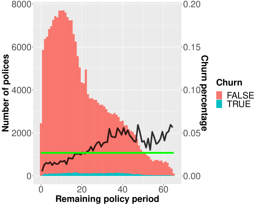
Figure 3: Number of canceled and non-cancelled contracts depending on the remaining contract term; the black line represents the lapse rate depending on the remaining contract duration, the green line represents the lapse rate of the entire annuity data set.

Insurance Sum

As can be seen in Figure 4, the higher the sum insured, the lower the proportion of canceled contracts. From an economic point of view, this makes sense, because a higher sum insured would lead to higher financial losses in the event of cancellation. In the case of private pension insurance, a low sum insured leads to a low monthly pension payment, which makes it less difficult to cancel the contract and invest the money elsewhere.

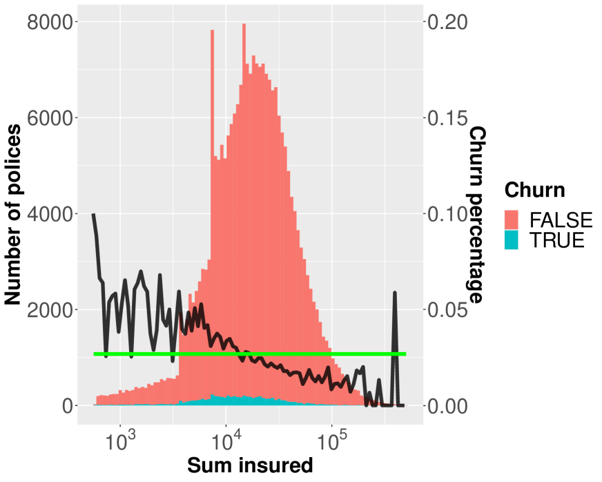
Figure 4: Number of canceled and non-cancelled contracts depending on the sum insured. The black line represents the lapse rate as a function of the sum insured, the green line the lapse rate of the entire annuity data set. The x-axis is plotted logarithmically.

5.2 Findings of Tuning

After the exploratory examination of the data, different settings of the models are investigated, which should finally provide the best model for each method.

Typically, for a random forest model, the more trees are trained, the better the model performance of such a model. Table 3 confirms this statement, because the higher the value of the hyper-parameter ntree, the better the model fit. On the other hand, the computational cost of a larger model compared to a smaller model is not necessarily proportional to the improvement in quality. Specifically, a random forest model using 300 trees will perform better, but not significantly better than the same model using only 50 trees. Nevertheless, the model must not be structured too simple. As can be seen in Table 3, a random forest model that uses only 10 trees performs substantially worse than a model with 50 trees.

osw.rate	ntree	ntry	nodesize	auc.te	auc.tr	bac.te	bac.tr	br.te	br.tr	f1.te	f1.tr
36	10	4	5000	0,7118	0,7454	0,6646	0,6854	0,2588	0,2394	0,0954	0,6927
36	50	4	5000	0,7250	0,7594	0,6690	0,6882	0,2502	0,2302	0,0962	0,6972
36	300	4	5000	0,7273	0,7640	0,6693	0,6890	0,2480	0,2285	0,0965	0,6977

Table 3: Performance difference of a random forest model depending on the hyper-parameter ntree. Exemplarily shown for the data set of the private pension; tr stands for training data and te for test data.

Another important aspect of this analysis is the handling or correction of the unbalanced target variable, i.e. the individual contract cancellation, in the data sets. Table 4 shows exemplarily for the random forest model that the oversampling rate osw.rate, i.e. by which factor the minority class is enlarged, has a direct positive impact on the model’s goodness-of-fit. Comparing the model without any adjustment of the training data, i.e. osw.rate $=1$, to models in which an adjustment was made, the model fit is significantly worse. It can be seen that an oversampling rate corresponding to the imbalance rate of a data set, i.e.

$$IR=\dfrac{N}{P},$$ (7)

yields the best performance. The imbalance rate describes the ratio of the minority to the majority class. At the same time, we find that a too strong correction of the imbalance reduces the model quality again.

osw.rate	ntree	ntry	nodesize	auc.te	auc.tr	bac.te	bac.tr	br.te	br.tr	f1.te	f1.tr
1	50	4	2500	0,5064	0,5244	0,5000	0,5000	0,0268	0,0267	0,0000	0,0000
18	50	4	2500	0,7150	0,7650	0,6071	0,6323	0,0726	0,2072	0,1386	0,4579
36	50	4	2500	0,7282	0,7920	0,6693	0,7116	0,2301	0,2063	0,0985	0,7209
54	50	4	2500	0,7203	0,8188	0,6599	0,7002	0,3468	0,1898	0,0828	0,8011

Table 4: Performance difference of a random forest model depending on the hyper-parameter osw.rate. Exemplarily shown for the data set of the private pension; tr stands for training data and te for test data.

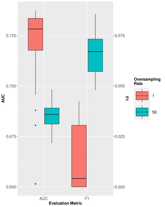
Figure 5: Performance of XGBoost models generated in tuning depending on the hyper-parameter sw.rate

We additionally compared the AUC and F1 performance metrics, which were calculated on external test data during the tuning of an XGBoost model for the ELI data set, see Figure 5. It is noticeable that XGBoost models without an oversampling adjustment in training achieve better AUC values than XGBoost models with an oversampling adjustment close to the imbalance rate (7). In addition, XGBoost models without an oversampling adjustment in training achieved a worse performance with respect to the F1 measure compared to models that use an oversampling rate corresponding to the imbalance rate (7).

In summary, different oversampling rates lead to different model performances and, depending on the used learning procedure and the employed oversampling rate, different models are to be preferred.

5.3 Performance

In this study, the employed models are based on different classification methods. The evaluation of the results of these models is done as described in Chapter 4.3. During the parameter tuning of these models, different parameter settings were tried and for each of them the corresponding test and training performances with respect to both performance measures were calculated.

Table 5 shows the best performance on external test data for each classification method and both goodness-of-fit measures. First of all, it can be observed that none of the models achieves a remarkable predictive performance, regardless of which data set is analyzed.

Comparing the values obtained in Table 5 with the benchmarks from Gold (2020), it can be concluded that the models achieve a moderate predictive performance. The goal would be to achieve e.g. an AUC of $0.8-0.85$, see Gold (2020).

A more detailed analysis reveals differences between the different learning methods. On the one hand, both the random forest and the XGBoost method achieve the best test performance values with respect to the measures AUC and, on the other hand, the Logit model shows the worst performance for all goodness-of-fit measures. For this reason, the logit models and CART models are no longer considered for the analysis of the variables in the further course. In addition to the analysis of the best test performance values, the other models will now be examined in more detail.

	Approach	AUC	F1
Endowment life insurance	Logit	0.6440	0.0522
	Elastic Net	0.6931	0.0985
	CART	0.7070	0.1002
	Random Forest	0.7221	0.1124
	XGBoost	0.7335	0.0779
Private pension insurance	Logit	0.6666	0.0946
	Elastic Net	0.7115	0.1226
	CART	0,7106	0.1263
	Random Forest	0.7333	0.1529
	XGBoost	0.7367	0.1405

Table 5: Overview of the best performances for different classification methods on external test data and for two different real data sets.

5.3.1 ROC-plots

Figures 6 and 7 show the ROC and Precison/Recall curves for the models that are optimal with respect to AUC. In Figures 6(a), 6(b), 7(a), and 7(b), the models were fitted in combination with random oversampling.

The course of the ROC curves neither indicates a solely random, and thus very bad, nor a very good model performance. Furthermore, all shown ROC curves, except for those corresponding to the logit models, are rather close to each other and show a very similar behavior, whereas the curves of the random forest and XGBoost models show a slightly better performance.

Looking at the Precision-Recall curves of the learning methods, all models show a rather poor performance for the (underrepresented) positive observations, since all curves run along the lower left corner.

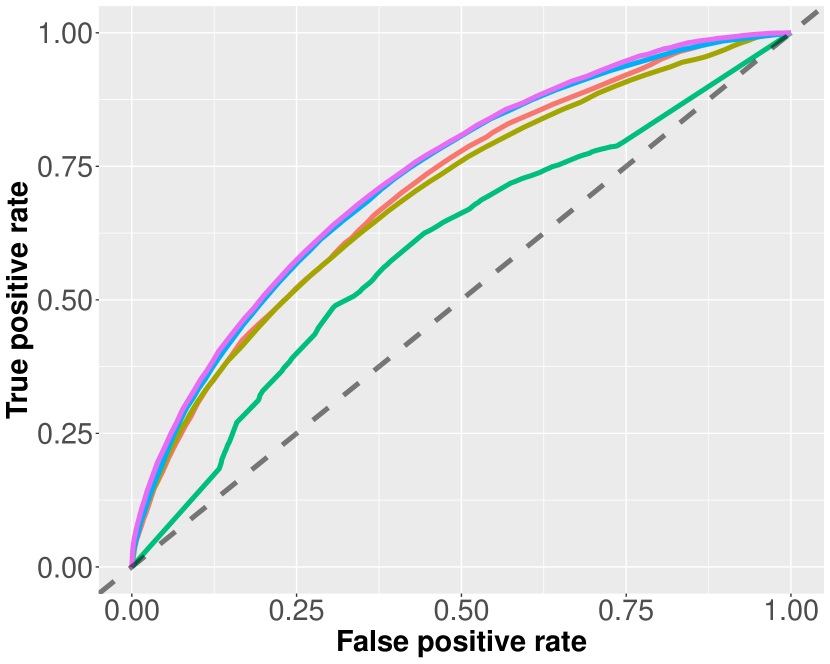
(a) ROC curves

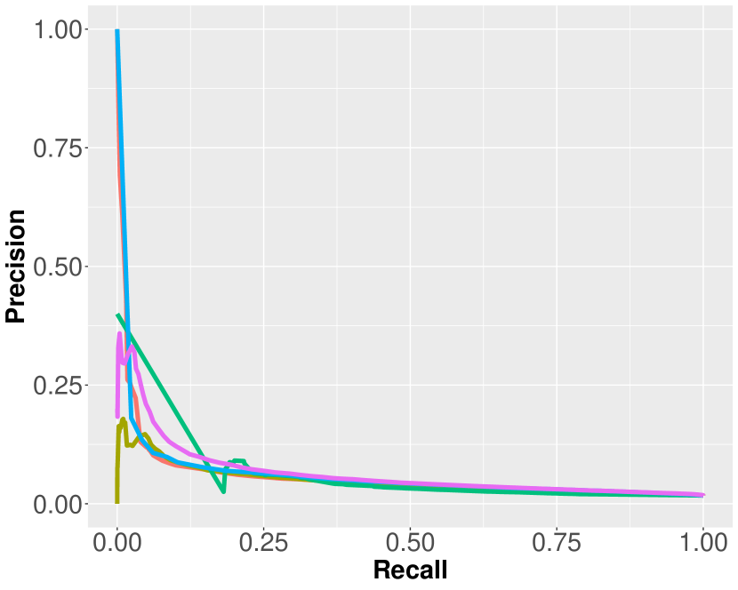
(b) PR curves

Figure 6: ROC and Precision-Recall curves for the endowment life insurance data set for the models that are optimal in terms of AUC. The models were computed using random oversampling as well as 10-fold cross-validation.
In Figures 6(a) and 6(b), the corresponding ROC and Precision-Recall curves (regarding cross-validation) are shown in an aggregated form.

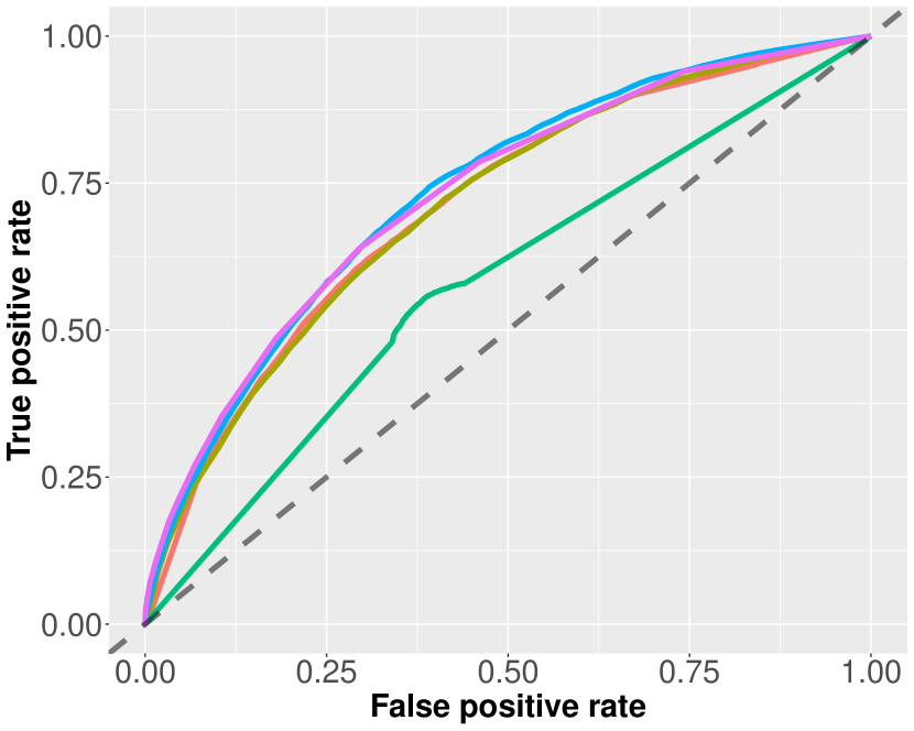
(a) ROC-kurven

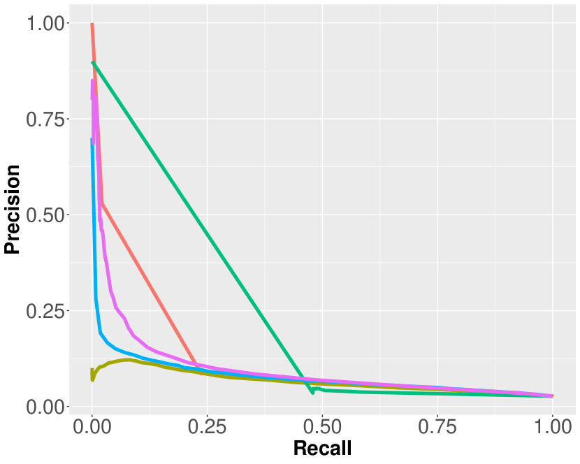
(b) PR-Kurven

Figure 7: ROC and Precision-Recall curves for the private pension data set for the models that are optimal in terms of AUC. The models were computed using random oversampling as well as 10-fold cross-validation.
In Figures 6(a) and 6(b) the corresponding ROC and Precision-Recall curves (regarding cross-validation) are shown in an aggregated form.

5.3.2 Variable Relevance

In addition to the ROC and Precision-Recall curves, methods for calculating the Variable Relevance were introduced in Section 4.4. With the help of these characteristics, the major research questions of this project can be answered, which concerns the determination of the concrete reasons and causes of lapse behavior for life insurance contracts. To answer this question, we examine in more detail those elastic net, random forest, and XGBoost models that are optimal with respect to AUC. For this purpose, we consider the corresponding variable relevance values of both data sets, which are displayed in Figure 8. The graph can be read as follows: The larger the respective symbol, the larger the corresponding value of variable relevance and thus the influence on the predictive power of a model.

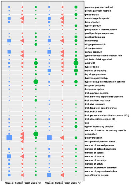
Figure 8: Variable relevances for three different classification approaches: XGBoost (blue & left), random forest (red & middle) and elastic net (green & right). The first three columns correspond to the data set of the private pension, columns 4-6 to the endowment insurance data set.

The predictors identified as most important via the concept of the introduced variable relevance methods can generally be grouped into three types for both examined data sets: Time-related influences, contract content, and information from the collection system.

• The temporal influences include information on the policy inception, the remaining policy period of a contract part, and the age of insured person.

• Important features related to the contract content are, for example, the contractually agreed sum insured and the annual premium paid. Especially for the private pension data set, also the occupation has been identified as an important feature.

• With regard to the information used from the collection system, the number of returns was found to be relevant, especially in the context of the private pension insurance data. Here, a return describes a payment request by the insurance company that has not been answered by the customer.

Principally, it turns out that all three approaches show a rather high agreement on both regarded data sets in terms of which variables are more or less relevant. We will now discuss our findings regarding the variable relevance of the different features in more detail. Using the variable relevance of all model types listed in Figure 8, it can be seen, for example, that the presence of a particular supplementary insurance will have little impact on the predictive validity, see characteristics of type ”incl. xxx”.

Some other variables such as the PricingID, the Method of financing, the BAV indicator (type of occupational pension scheme), or the profit participation turn out to be quite important in some models, whereas they appear to be of little relevance in others. It must be emphasized, however, that most of the predictors that are relevant for the predictive performance within one model also exhibit some importance in other models. For a large subset of these features, this statement can even be made for both data sets, which allows us to infer that these features have a high influence on individual policy lapses for at least the regarded two product types of life insurance. It should also be emphasized that these findings confirm the aspects identified in Section 5.1, e.g. a strong influence of the remaining contract duration or the sum insured.

All in all, however, the computed models unfortunately only achieve a limited degree of predictive accuracy. Against this background, it is important to note that the predictors identified as particularly important by the variable relevance methods are not necessarily the most important predictors that generally exist. In other words, other possibly important features have not been included in the data and models used in this study (see Section 6 for a discussion of candidate covariates).

6 Conclusion and outlook

In the present study, we investigated how well the portfolio data of a large German life insurance company can be used to predict and explain individual contract cancellation behavior.

For this purpose, data from endowment life insurance and private pensions were used and processed. Furthermore, some forecasting methods were presented in the manuscript, which were subsequently applied to these data sets.

As a starting point the date 1/1/2018 was chosen. Then, the inventory data of the two products described above were used, which were combined with the cancellation data of the year 2018. Thus, it was possible to determine for each contract in the insurer’s portfolio as of 1/1/2018 whether it had been terminated by lapse at the end of the year.

For each product, only the main insurance of the contract was considered. Information about the customer, time components, information about additional insurances and some other details from the collection system were added to the usual contract data. This resulted in data sets for both products with a sufficient number of features to apply different prediction methods.

In addition to classical logistic models, which included the standard logit model and an elastic net-regularized version of it, tree-based methods such as CART, random forest and XGBoost were also used. Based on these methods, a large number of models per insurance product was considered and the best model was selected based on tuning strategies. For the tree-based methods, parameters such as the number of trees, the depth of the trees, the size of the nodes and the oversampling rate were considered in the tuning process. The last tuning parameter was particularly relevant here, as life insurance contracts naturally are rarely cancelled and thus, there were few cancelled as opposed to non-cancelled contracts. This unbalancedness of our data sets was taken into account by using an oversampling approach, so-called random oversampling.

The analysis of the models using ROC and precision-recall plots clearly showed that the cancellation behavior of individual contracts could only be explained moderately well on the basis of the available data. None of the classification methods investigated in this project substantially outperformed the others or achieved a very satisfactory predictive accuracy.

The concept of variable relevance, which was used to analyze and interpret the individual contract cancellation behavior, finally showed that some temporal components, such as the start of the contract, the remaining duration of the contract or the age of the first insured person, but also certain contract contents, such as the sum insured, the annual premiums paid, the surplus system used, as well as information from the collection system, primarily the number of repayments, had a substantial influence on the prediction. Since the values of the model’s goodness-of-fit are neither particularly bad or good, these findings should be viewed with some caution.

As an outlook and extension to this work, two major steps can be considered in further research: Incorporating additional data sources or using other models, such as e.g. boosting approaches or deep learning methods such as neural networks.

Other data sources

The incorporation of additional data sources always requires the inclusion of data protection regulations, so that both the extraction and further use of additional covariate data can be done in compliance with the law. Possible data sources that could provide essential information within the focus of this study are

• The company’s stored correspondence with the customer
   
  In the future, for example, information on customer satisfaction, on the cause of various steps taken, or additional personal customer information could be extracted from various data sources available to the life insurance company, e.g. via using text mining methods. This information could then be added to the data records, thereby increasing the number of features, and thus the information content.

• All existing customer contracts
   
  This additional information could provide insight into whether customers who hold several different insurance contracts with the company have a different individual contract cancellation behavior than customers who are not that deeply rooted with the company. Changes such as cancellations or re-signings of other contracts may have a direct impact on the contracts under investigation.

• Extraction of customer information from social media platforms
   
  Data from social media platforms is a modern and widely used field of analysis in other industries to analyze changes in private relationships.

Other modeling approaches

In this manuscript, solely classification methods have been considered. A possible extension could be to focus more on temporal effects in the future. Then, models from the field of time series analysis or time-to-event analysis could be considered. The fact that temporal information plays an important role in the models considered in this work could be interpreted as a first hint to indeed further pursue this idea. One problem that arises, for example, for models from time series analysis is the creation of a meaningful data basis. The content of this data basis should be time series that show the historical course of a contract. However, since these are not always available in the desired quality, this turn out to be an insurmountable hurdle.

In conclusion, it can be stated that statistical analyses in the field of insurance company portfolio management can be promising, but as also shown in the present manuscript, could arise some problems. Some of these problems can be addressed and potentially solved, while for others the effort involved in their solution is not commensurate with the associated added value.

References

- Bentéjac et al. (2021) Bentéjac, C., A. Csörgő, and G. Martínez-Muñoz (2021). A comparative analysis of gradient boosting algorithms. Artificial Intelligence Review 54(3), 1937–1967.
- Bischl et al. (2016) Bischl, B., M. Lang, L. Kotthoff, J. Schiffner, J. Richter, E. Studerus, G. Casalicchio, and Z. Jones (2016). mlr: Machine learning in r. Journal of Machine Learning Research 17(170), 1–5.
- Bradley (1997) Bradley, A. P. (1997). The use of the area under the roc curve in the evaluation of machine learning algorithms. Pattern recognition 30(7), 1145–1159.
- Breiman (2001) Breiman, L. (2001). Random forests. Machine learning 45, 5–32.
- Breiman et al. (1984) Breiman, L., J. Friedman, C. J. Stone, and R. . Olshen (1984). Classification And Regression Trees.
- Chawla et al. (2002) Chawla, N. V., K. W. Bowyer, L. O. Hall, and W. P. Kegelmeyer (2002). Smote: Synthetic minority over-sampling technique. Journal of Artificial Intelligence Research 16, 321–357.
- Chen and Guestrin (2016) Chen, T. and C. Guestrin (2016). Xgboost: A scalable tree boosting system. In Proceedings of the 22nd acm sigkdd international conference on knowledge discovery and data mining, pp. 785–794.
- Davis and Goadrich (2006) Davis, J. and M. Goadrich (2006). The relationship between precision-recall and roc curves. In Proceedings of the 23rd International Conference on Machine Learning, ICML ’06, pp. 233–240.
- Denuit et al. (2021) Denuit, M., A. Charpentier, and J. Trufin (2021). Autocalibration and tweedie-dominance for insurance pricing with machine learning. Insurance: Mathematics and Economics 101, 485–497.
- Devriendt et al. (2021) Devriendt, S., K. Antonio, T. Reynkens, and R. Verbelen (2021). Sparse regression with multi-type regularized feature modeling. Insurance: Mathematics and Economics 96, 248–261.
- Distributed Machine Learning Community (2021) Distributed Machine Learning Community (2021). Machine learning challenge winning solutions. https://github.com/dmlc/xgboost/tree/master/demo#machine-learning-challenge-winning-solutions. (Accessed on 05.10.2014).
- Fahrmeir et al. (2013) Fahrmeir, L., T. Kneib, S. Lang, and B. Marx (2013). Regression: Models, Methods and Applications. Springer-Verlag.
- Fahrmeir and Tutz (2001) Fahrmeir, L. and G. Tutz (2001). Multivariate Statistical Modelling Based on Generalized Linear Models. Springer.
- Fawcett (2006) Fawcett, T. (2006). An introduction to roc analysis. Pattern Recognition Letters 27(8), 861–874.
- Fernández et al. (2018) Fernández, A., S. García, M. Galar, R. C. Prati, B. Krawczyk, and F. Herrera (2018). Learning from Imbalanced Data Sets.
- Friedman et al. (2010) Friedman, J., T. Hastie, and R. Tibshirani (2010). Regularization paths for generalized linear models via coordinate descent. Journal of statistical software 33(1), 1–22.
- Friedman (2001) Friedman, J. H. (2001). Greedy function approximation: A gradient boosting machine. The Annals of Statistics 20(5), 1189–1232.
- Gan (2013) Gan, G. (2013). Application of data clustering and machine learning in variable annuity valuation. Insurance: Mathematics and Economics 53(3), 795–801.
- Goadrich et al. (2006) Goadrich, M., L. Oliphant, and J. Shavlik (2006). Gleaner: Creating ensembles of first-order clauses to improve recall-precision curves. Machine Learning 64(1-3), 231–261.
- Gold (2020) Gold, C. S. (2020). Fighting Churn with Data: The science and strategy of customer retention. Manning Publications.
- Hanley and McNeil (1983) Hanley, J. A. and B. J. McNeil (1983). A method of comparing the areas under receiver operating characteristic curves derived from the same cases. Radiology 148(3), 839–843.
- Hastie et al. (2009) Hastie, T., R. Tibshirani, and J. Friedman (2009). The Elements of Statistical Learning: Data Mining, Inference, and Prediction.
- He and Garcia (2009) He, H. and E. A. Garcia (2009). Learning from imbalanced data. IEEE Transactions on Knowledge and Data Engineering 21(9), 1263 – 1284.
- He and Ma (2013) He, H. and Y. Ma (2013). Imbalanced Learning: Foundations, Algorithms, and Applications.
- Hoerl and Kennard (1970) Hoerl, A. E. and R. W. Kennard (1970). Ridge regression: Biased estimation for nonorthogonal problems. Technometrics 12(1), 55–67.
- Makariou et al. (2021) Makariou, D., P. Barrieu, and Y. Chen (2021). A random forest based approach for predicting spreads in the primary catastrophe bond market. Insurance: Mathematics and Economics 101, 140–162.
- McCullagh and Nelder (2019) McCullagh, P. and J. A. Nelder (2019). Generalized Linear Models. Routledge.
- Meier et al. (2008) Meier, L., S. Van De Geer, and P. Bühlmann (2008). The group lasso for logistic regression. Journal of the Royal Statistical Society: Series B (Statistical Methodology) 70(1), 53–71.
- Ortmann (2009) Ortmann, K. (2009). Praktische Lebensversicherungsmathematik. Springer.
- R Core Team (2020) R Core Team (2020). R: A Language and Environment for Statistical Computing. Vienna, Austria: R Foundation for Statistical Computing.
- Tibshirani (1996) Tibshirani, R. (1996). Regression shrinkage and selection via the lasso. Journal of the Royal Statistical Society: Series B (Methodological) 58(1), 267–288.
- Zou and Hastie (2005) Zou, H. and T. Hastie (2005). Regularization and variable selection via the elastic net. Journal of the Royal Statistical Society: Series B (Statistical Methodology) 67(2), 301–320.