Space4HGNN: A Novel, Modularized and Reproducible Platform to Evaluate Heterogeneous Graph Neural Network
Abstract.
Heterogeneous Graph Neural Network (HGNN) has been successfully employed in various tasks, but we cannot accurately know the importance of different design dimensions of HGNNs due to diverse architectures and applied scenarios. Besides, in the research community of HGNNs, implementing and evaluating various tasks still need much human effort. To mitigate these issues, we first propose a unified framework covering most HGNNs, consisting of three components: heterogeneous linear transformation, heterogeneous graph transformation, and heterogeneous message passing layer. Then we build a platform Space4HGNN by defining a design space for HGNNs based on the unified framework, which offers modularized components, reproducible implementations, and standardized evaluation for HGNNs. Finally, we conduct experiments to analyze the effect of different designs. With the insights found, we distill a condensed design space and verify its effectiveness.
1. Introduction
In information retrieval, graph neural network (GNN) as graph learning and representation method has been applied in recommendation (Chang et al., 2020; Wang et al., 2019a; Chen et al., 2021b; Chang et al., 2021; Zhao et al., 2017) and knowledge representation (Gong et al., 2020; Cao et al., 2021; Hao et al., 2020; Mei et al., 2018). Most GNNs focus on homogeneous graphs, while more and more research (Schlichtkrull et al., 2018; Wang et al., 2019b; Jin et al., 2020; Fang et al., 2019; Yu et al., 2021) shows that real world with complex interactions, e.g., social network (Tang et al., 2008; Wang et al., 2019c), can be better modeled by heterogeneous graphs (a.k.a., heterogeneous information networks). Taking recommender system as an example, it can be regarded as a bipartite graph consisting of users and items, and a lot of auxiliary information also has a complex network structure, which can be naturally modeled as a heterogeneous graph. Besides, some works (Guo and Liu, 2015; Liu et al., 2020; Bi et al., 2020; Jiang et al., 2018; Ghazimatin, 2020; Fan et al., 2019; Li et al., 2020; Chen et al., 2021a) have achieved state-of-the-art (SOTA) performance by designing heterogeneous graph neural network (HGNN). In fact, HGNNs can utilize the complex structure and rich semantic information (Wang et al., 2020), and have been widely applied in many fields, such as e-commerce (Zhao et al., 2019; Ji et al., 2021b), and security (Sun et al., 2020; Hu et al., 2019).
| Neighbors | One-hop | Meta-path | ||
| Model Family | Homogenization | Relation | Meta-path | |
| Heterogeneous Graph Transformation | Homogenization of the heterogeneous graph | Relation subgraph extraction | Meta-path subgraph extraction | |
| Heterogeneous Message Passing | Direct-aggregation | Dual-aggregation | ||
| Graph Convolution | Single graph homogeneous convolution | Single graph heterogeneous convolution | Multiple homogeneous graph convolutions applied to different subgraphs | |
| Model | GCN (Kipf and Welling, 2017), GAT (Veličković et al., 2018), GraphSage (Hamilton et al., 2017), GIN (Xu et al., 2019) | HGAT (Linmei et al., 2019), HetSANN (Hong et al., 2020) HGT (Hu et al., 2020), Simple-HGN (Lv et al., 2021) | RGCN (Schlichtkrull et al., 2018), HGConv (Yu et al., 2020) | HAN (Wang et al., 2019b), HPN (Ji et al., 2021a) |
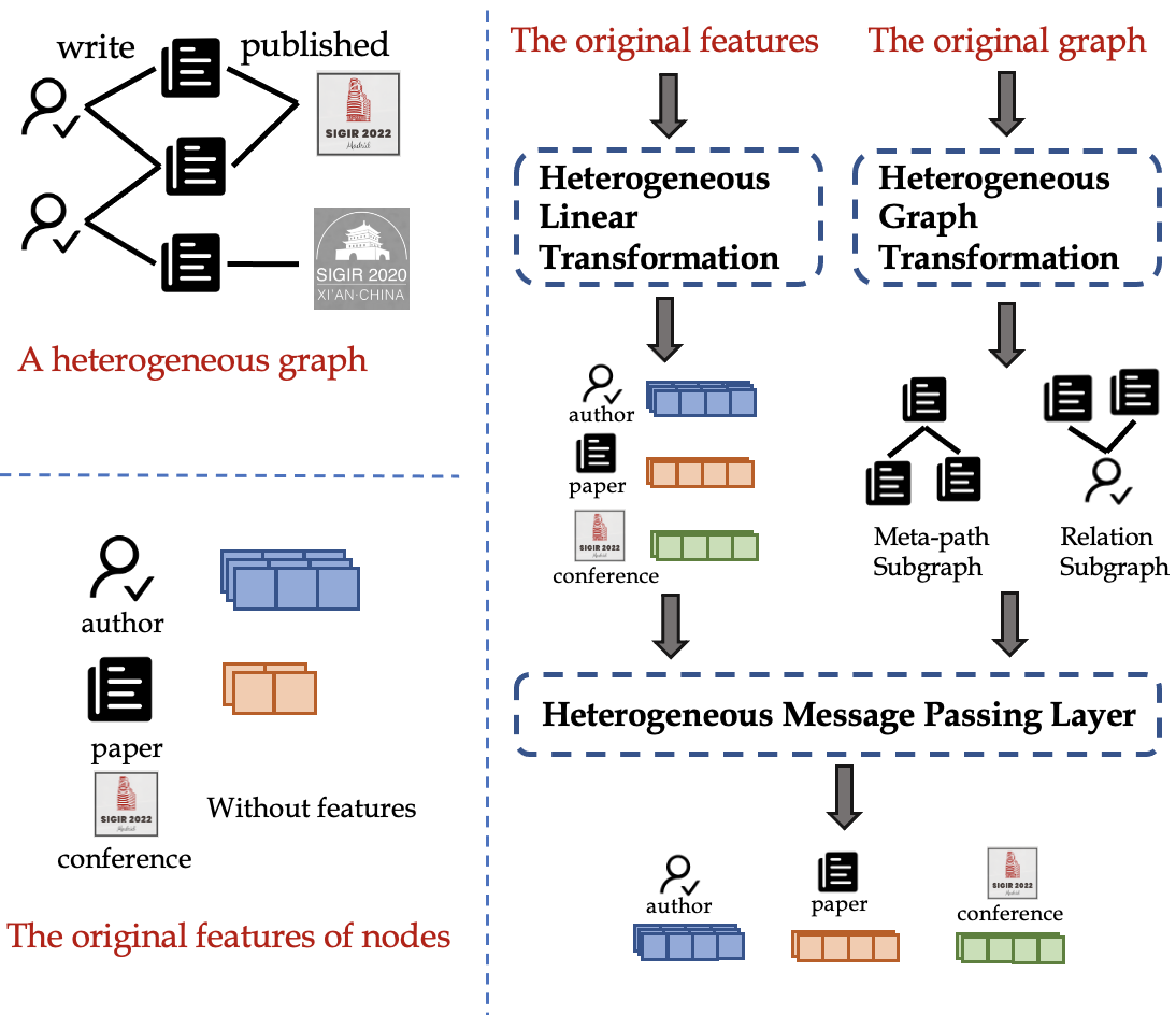
However, it is increasingly difficult for researchers in the field to compare existing methods and contribute with novel ones. The reason is that previous evaluations are conducted from the point of view of model-level, and we cannot accurately know the importance of each component due to diverse architecture designs and applied scenarios. To evaluate them from the sight of module-level, we first propose a unified framework of existing HGNNs that consists of three key components through systematically analyzing their underlying graph data transformation and aggregation procedures, as shown in Figure 1 (right). The first component Heterogeneous Linear Transformation is a general operation of HGNNs, which maps features to a shared feature space. Summarizing the transformed graphs used in different HGNNs, we abstract the second component Heterogeneous Graph Transformation containing relation subgraph extraction, meta-path subgraph extraction, and homogenization of the heterogeneous graph. With that, we can explicitly decouple the selection procedure of receptive field and message passing procedure. Hence the third component Heterogeneous Message Passing Layer can focus on the key procedure involving diverse graph convolution layers. As shown in Table 1, our framework both categorizes existing approaches and facilitates the exploration of novel ones.
With the help of the unified framework, we propose to define a design space for HGNNs, which consists of a Cartesian product of different design dimensions following GraphGym (You et al., 2020). In GraphGym, there have been analysis results of design dimensions for GNNs, which is not enough for HGNNs. To figure out whether the guidelines distilled from GNNs are effective, our design space still contains common design dimensions with GraphGym. Besides, to capture heterogeneity, we distill three model families according to Heterogeneous Graph Transformation in our unified framework. Based on the design space, we build a platform Space4HGNN 111https://github.com/BUPT-GAMMA/Space4HGNN, which offers reproducible model implementation, standardized evaluation for diverse architecture designs, and easy-to-extend API to plug in more architecture design options. We believe Space4HGNN can greatly facilitate the research field of HGNNs. Specifically, we could check the effect of the tricky designs or architecture design quickly, innovate the HGNN models easily, and apply HGNN in other interesting scenarios. In addition, the platform can be used as the basis of neural architecture search for HGNNs in future work.
With the platform Space4HGNN, we conduct extensive experiments and aim to analyze the design dimensions. We first evaluate common design dimensions used in GraphGym with uniform random search, and find that they are partly effective in HGNNs. More importantly, to accurately judge the diverse architecture designs in HGNNs, we comprehensively analyze unique design dimensions in HGNNs. And we sum up the following insights:
-
•
Different model families have different suitable scenarios. The meta-path model family has an advantage in node classification task, and the relation model family performs outstandingly in link prediction task.
-
•
The preference for different design dimensions may be opposite in different tasks. For example, node classification task prefers to apply L2 Normalization and remove Batch Normalization. However, the better choices of the same datasets for link prediction task are the opposite.
-
•
We should select graph convolution carefully which varies greatly across datasets. Besides, the design dimensions like the number of message passing layers, hidden dimension and dropout are all important.
Finally, we distill a condensed design space according to the analysis results, whose scale is reduced by 500 times. We evaluate it in a new benchmark HGB (Lv et al., 2021) and demonstrate the effectiveness of the condensed design space.
And we sum up the following contributions:
-
•
As far as we know, we are the first to propose a unified framework and define a design space for HGNNs. They offer us a module-level sight and help us evaluate the influences of different design dimensions, such as high-level architectural designs, and design principles.
-
•
We release a platform Space4HGNN for design space in HGNNs, which offers modularized components, standardized evaluation, and reproducible implementation of HGNN. We conduct extensive experimental evaluations to analyze HGNNs comprehensively, and provide findings behind the results based on Space4HGNN. It allows researchers to find more interesting findings and explore more robust and generalized models.
-
•
Following the findings, we distill a condensed design space. Experimental results on a new benchmark HGB (Lv et al., 2021) show that we can easily achieve state-of-the-art performance with a simple random search in the condensed space.
2. Related Work
Notations and the corresponding descriptions used in the rest of the paper are given in Table 2. More preliminaries can be found in Appendix A.
| Notation | Description |
| The node | |
| The edge from node to node | |
| The neighbors of node | |
| The hidden representation of a node | |
| The trainable weight matrix | |
| The node type mapping function | |
| The edge type mapping function | |
| The message function |
2.1. Heterogeneous Graph Neural Network
Different from GNNs, HGNNs need to handle the heterogeneity of structure and capture rich semantics of heterogeneous graphs. According to the strategies of handling heterogeneity, HGNN can be roughly classified into two categories: HGNN based on one-hop neighbor aggregation (similar to traditional GNN) and HGNN based on meta-path neighbor aggregation (to mine semantic information), shown in Table 1.
2.1.1. HGNN based on one-hop neighbor aggregation
To deal with heterogeneity, this kind of HGNN usually contains type-specific convolution. Similar to GNNs, the aggregation procedure occurs in one-hop neighbors. As earliest work and an extension of GCN (Kipf and Welling, 2017), RGCN (Schlichtkrull et al., 2018) assigns different weight matrices to different relation types and aggregates one-hop neighbors. With many GNN variants appearing, homogeneous GNNs inspire more HGNNs and then HGConv (Yu et al., 2020) dual-aggregate one-hop neighbors based on GATConv (Veličković et al., 2018). A recent work SimpleHGN (Lv et al., 2021) designs relation-type weight matrices and embeddings to characterize the heterogeneous attention over each edge. Besides, some earlier models, like HGAT (Linmei et al., 2019), HetSANN (Hong et al., 2020), HGT(Hu et al., 2020), modify GAT (Veličković et al., 2018) with heterogeneity by assigning heterogeneous attention for either nodes or edges.
2.1.2. HGNN based on meta-path neighbor aggregation
Another class of HGNNs is to capture higher-order semantic information with hand-crafted meta-paths. Different from the previous, aggregation procedure occurs in neighbors connected by meta-path. As a pioneering work, HAN (Wang et al., 2019b) first uses node-level attention to aggregate nodes connected by the same meta-path and utilizes semantic-level attention to fuse information from different meta-paths. Because the meta-path subgraph ignores all the intermediate nodes, MAGNN (Fu et al., 2020) aggregates all nodes in meta-path instances to ensure that information will not be missed. Though meta-paths contain rich semantic information, the selection of meta-paths needs human prior and determines the performance of HGNNs. Some works like GTN (Yun et al., 2019) learn meta-paths automatically to construct a new graph. HAN (Wang et al., 2019b) and HPN (Ji et al., 2021a), which are easy to extend, will be included in our framework for generality.
2.2. Model Evaluation and Design Space
There are many works to measure progress in the field by evaluating models. The work (Dacrema et al., 2019) reports the results of a systematic analysis of neural recommendation mentioning HGNNs and sheds light on potential problems. Several works (Errica et al., 2020; Dwivedi et al., 2020; Shchur et al., 2018) discuss how to make fair a comparison between GNN models. In HGNNs, a recent work (Lv et al., 2021) revisits HGNNs and proposes issues with existing HGNNs. The above work is to evaluate models from the model-level sight.
Though rigorous theoretical understanding of neural network is not enough, it is imperative to perform empirical studies of neural network to discover better architectures. In visual recognition, some works (Radosavovic et al., 2019, 2020)design network design spaces to help advance the understanding of network design and discover design principles that generalize across settings. Inspired by that, GraphGym (You et al., 2020) proposes a GNN design space and a GNN task space to evaluate model-task combinations comprehensively. In recommendation system, the work (Wang et al., 2022) profiles the design space for GNNs based on collaborative filtering.
Here we aim to extensively explore the design space of HGNNs involving many design dimensions and evaluate different design architectures. Different from the model-level sight of (Lv et al., 2021), we evaluate the design dimensions from module-level sight and distill helpful design principles. Different from GraphGym (You et al., 2020), our design space focuses on the unique design dimension of HGNNs and explores the differences with GNNs.
3. A Unified Framework of Heterogeneous Graph Neural Network
As shown in Table 1, we categorize many mainstream HGNN models, which could be applied in many scenarios, e.g, link prediction (Hao et al., 2020; Mei et al., 2018) and recommendation (Bi et al., 2020; Jiang et al., 2018; Ghazimatin, 2020). Through analyzing the underlying graph data and the aggregation procedure of existing HGNNs, we propose a unified framework of HGNN that consists of three main components:
-
•
Heterogeneous Linear Transformation maps features or representations with heterogeneity to a shared feature space.
-
•
Heterogeneous Graph Transformation offers four transformation methods for heterogeneous graph data to select the receptive field.
-
•
Heterogeneous Message Passing Layer defines two aggregation methods suitable for most HGNNs.
3.1. Heterogeneous Linear Transformation
Due to the heterogeneity of nodes, different types of nodes have different semantic features even different dimensions. Therefore, for each type of nodes (e.g., node with node type ), we design a type-specific linear transformation to project the features (or representations) of different types of nodes to a shared feature space. The linear transformation is shown as follows:
| (1) |
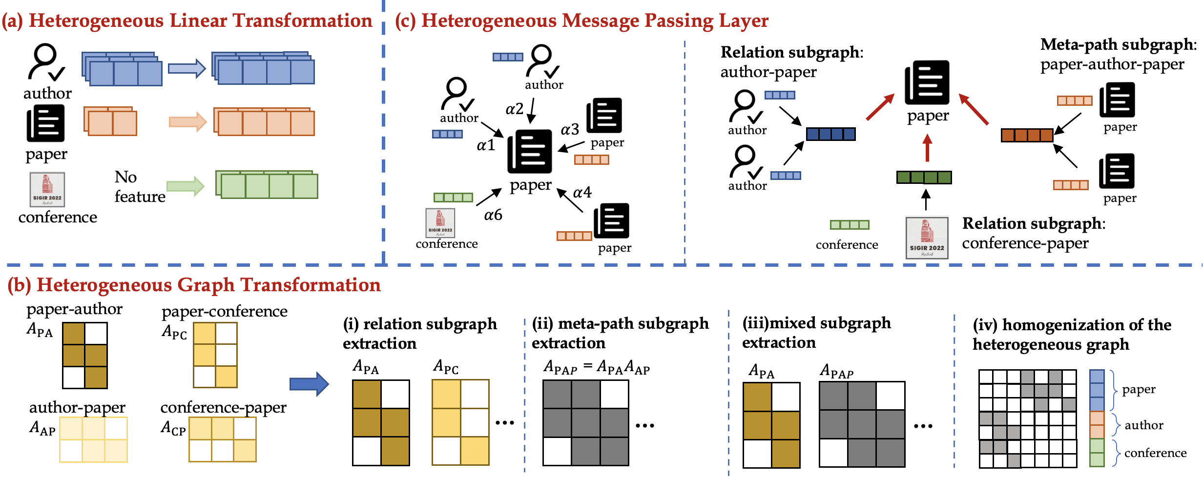
where and are the original and projected feature of node, respectively. As shown in Figure 2 (a), we transform node features with a type-specific linear transformation for nodes with features. Nodes without features or full of noise could be assigned embeddings as trainable vectors, which is equivalent to assigning them with a one-hot vector combined with a linear transformation.
3.2. Heterogeneous Graph Transformation
In previous work, aggregation based on one-hop neighbor usually applies the graph convolution layer in the original graph, which implicitly selects the one-hop (relation) receptive field. And aggregation based on meta-path neighbor is usually done on constructed meta-path subgraphs, which explicitly selects the multi-hop (meta-path) receptive field. Relation subgraphs are special meta-path subgraphs (note that the original graph is a special case of relation subgraphs). To unify both, we propose a component to abstract the selection procedure of the receptive field, which determines which nodes are aggregated. Besides, the component decouples the selection procedure of receptive field and message passing procedure introduced in the following subsection.
As shown in Figure 2 (b), we therefore designate a separate stage called Heterogeneous Graph Transformation for graph construction, and categorize it into (i) relation subgraph extraction that extracts the adjacency matrices of the specified relations, (ii) meta-path subgraph extraction that constructs the adjacency matrices based on the pre-defined meta-paths, (iii) mixed subgraph extraction that builds both kinds of subgraphs, (iv) homogenization of the heterogeneous graph (but still preserving and for node and edge type mapping). For relation or meta-path extraction, we could construct subgraphs by specifying relation types or pre-defined meta-paths.
3.3. Heterogeneous Message Passing Layer
In Section 2.1, we introduce a conventional way to classify HGNNs. However, this classification did not find enough commonality from the implementation perspective, resulting in difficulties in defining design space and searching for new models. Therefore, we instead propose to categorize models by their aggregation methods.
3.3.1. Direct-aggregation
The aggregation procedure is to reduce neighbors directly without distinguishing node types. The basic baselines of HGNN models are GCN, GAT, and other GNNs used in the homogeneous graph. A recent work(Lv et al., 2021) shows that the simple homogeneous GNNs, e.g., GCN and GAT, are largely underestimated due to improper settings.
As shown in Figure 2 (c: the left one), we will explain it under the message passing GNNs formulation and take GAT (Veličković et al., 2018) as an example. The message function is . The feature of node in -th layer is defined as
| (2) |
where is a trainable weight matrix, is neighbors of node and is the normalized attention coefficients between node and , defined by that:
| (3) |
The correlation of node with its neighbor is represented by attention coefficients . Changing the form of yields other heterogeneous variants of GAT, which we summarize in Table 3.
3.3.2. Dual-aggregation
Following (Yu et al., 2020), we define two parts of dual-aggregation: micro-level (intra-type) and macro-level (inter-type) aggregation. As shown in Figure 2 (c: the right one), micro-level aggregation is to reduce node features within the same relation, which generate type-specific features in relation/meta-path subgraphs, and macro-level aggregation is to reduce type-specific features across different relations. When multiple relations have the same destination node types, their type-specific features are aggregated by the macro-level aggregation.
Generally, each relation/meta-path subgraph utilizes the same micro-level aggregation (e.g., graph convolution layer from GCN or GAT). In fact, we can apply different homogeneous graph convolutions for different subgraphs in our framework. The multiple homogeneous graph convolutions combined with macro-level aggregation is another form of heterogeneous graph convolution compared with heterogeneous graph convolution in direct-aggregation. There is a minor difference between the heterogeneous graph convolution of direct-aggregation and that of dual-aggregation. We modify Eq. 3 and define it in Eq. 4, where means the neighbors type of node is the same as type of node .
| (4) |
Example: HAN (Wang et al., 2019b) and HGConv (Yu et al., 2020). In HAN, the node-level attention is equivalent to a micro-level aggregation with GATConv, and the semantic-level attention is macro-level aggregation with attention, which is the same with HGConv. The HGConv uses the relation subgraphs, which means aggregating the one-hop neighbors, but HAN extracts multiple meta-path subgraphs, which means aggregating multi-hop neighbors. According to Heterogeneous Graph Transformation in Section 3.2, the graph constructed can be a mixture of meta-path subgraphs and relation subgraphs. So the dual-aggregation can also be operated in a mixture custom of subgraphs to aggregate different hop neighbors.
4. Design Space for Heterogeneous Graph Neural Network
Inspired by GraphGym (You et al., 2020), we propose a design space for HGNN, which is built as a platform Space4HGNN offering modularized HGNN implementation for researchers introduced at last.
4.1. Designs in HGNN
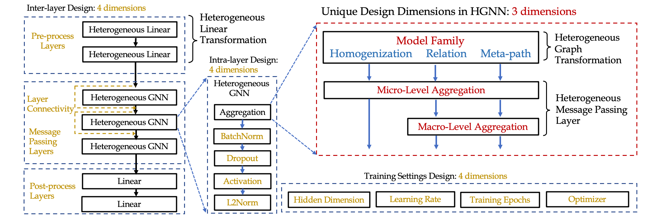
As illustrated in Figure 3, we will describe it from two aspects: common designs with GraphGym and unique designs distilled from HGNNs.
| Design Dimension | Choices |
| Batch Normalization | True, False |
| Dropout | 0, 0.3, 0.6 |
| Activation | Relu, LeakyRelu, Elu, Tanh, PRelu |
| L2 Normalization | True, False |
| Layer Connectivity | STACK, SKIP-SUM, SKIP-CAT |
| Pre-process Layers | 1, 2, 3 |
| Message Passing Layers | 1, 2, 3, 4, 5, 6 |
| Post-process Layers | 1, 2, 3 |
| Optimizer | Adam, SGD |
| Learning Rate | 0.1, 0.01, 0.001, 0.0001 |
| Training Epochs | 100, 200, 400 |
| Hidden dimension | 8, 16, 32, 64, 128 |
4.1.1. Common Designs with GraphGym
4.1.2. Unique Design in HGNNs
With the unified framework, we try to transform the modular components into unique design dimensions in HGNNs. According to (Radosavovic et al., 2019), a collection of related neural network architectures, typically sharing some high-level architectural structures or design principles (e.g., residual connections), could be abstracted into a model family. With that, we distill three model families in HGNNs.
| Design Dimension | Choices |
| Model Family | Homogenization, Relation, Meta-path |
| Micro-level Aggregation (Graph Convolution Layer) | GCNConv, GATConv, SageConv, GINConv |
| Macro-level Aggregation | Mean, Max, Sum, Attention |
The Homogenization Model Family
The homogenization model family uses the direct-aggregation combined with any graph convolutions. Here we use the term homogenization because all HGNNs included here apply direct-aggregation after the homogenization of the heterogeneous graph mentioned in Section 3.2. Homogeneous GNNs and heterogeneous variants of GAT mentioned in Section 3.3 all fall into this model family. The homogeneous GNNs are usually evaluated as basic baselines in HGNN papers. Though it losses type information, it is confirmed that the simple homogeneous GNNs can outperform some existing HGNNs (Lv et al., 2021), which means they are nonnegligible and supposed to be seen as a model family. We select four typical graph convolution layers, which are GraphConv (Kipf and Welling, 2017), GATConv (Veličković et al., 2018), SageConv-mean (Hamilton et al., 2017) and GINConv(Xu et al., 2019) as analyzed candidates.
The Relation Model Family
The model family applies relation subgraph extraction and dual-aggregation. The first HGNN model RGCN (Schlichtkrull et al., 2018) is a typical example in relation model family, whose dual-aggregation consists of a micro-level aggregation with SageConv-mean and macro-level aggregation of Sum. HGConv (Yu et al., 2020) is a combination of GATConv and attention. We could get other designs by enumerating the combinations of micro-level and macro-level aggregation. In our experiments, we set the micro-level aggregations the same as graph convolutions in the homogenization model family, and macro-level aggregations are chosen among Mean, Max, Sum, and Attention.
The Meta-path Model Family
The model family applies meta-path subgraph extraction and dual-aggregation. The instance HAN (Wang et al., 2019b) has the same dual-aggregation with HGConv (Yu et al., 2020) in the relation model family but different subgraph extraction. The candidate of micro-level and macro-level aggregations is the same as those in the relation model family.
4.2. Space4HGNN: Platform for Design Space in HGNN
We developed Space4HGNN, a novel platform for exploring HGNN designs. We believe Space4HGNN can significantly facilitate the research field of HGNNs. It is implemented with PyTorch 222https://pytorch.org/ and DGL 333https://github.com/dmlc/dgl, using the OpenHGNN 444https://github.com/BUPT-GAMMA/OpenHGNN package. It also offers a standardized evaluation pipeline for HGNNs, much like (You et al., 2020) for homogeneous GNNs. For faster experiments, we offer parallel launching. Its highlights are summarized below.
4.2.1. Modularized HGNN Implementation
The implementation closely follows the GNN design space GraphGym. It is easily extendable, allowing future developers to plug in more choices of design dimensions (e.g., a new graph convolution layer or a new macro-aggregation). Additionally, it is easy to import new design dimensions to Space4HGNN, such as score function in link prediction.
4.2.2. Standardized HGNN Evaluation
Space4HGNN offers a standardized evaluation pipeline for diverse architecture designs and HGNN models. Benefiting from OpenHGNN, we can evaluate diverse datasets in different tasks easily and offer visual comparison results presented in Section 5.
| Dataset | #Nodes | #Node Types | #Edges | #Edge Types | Name for Node Classification Task | Name for Link Prediction Task |
| DBLP | 26,128 | 4 | 239,566 | 6 | HGBn-DBLP | HGBl-DBLP |
| IMDB | 21,420 | 4 | 86,642 | 6 | HGBn-IMDB | HGBl-IMDB |
| ACM | 10,942 | 4 | 547,872 | 8 | HGBn-ACM | HGBl-ACM |
| Freebase | 180,098 | 8 | 1,057,688 | 36 | HGBn-Freebase | - |
| PubMed | 63,109 | 4 | 244,986 | 10 | HGBn-PubMed | HGBl-PubMed |
| Amazon | 10,099 | 1 | 148,659 | 2 | - | HGBl-amazon |
| LastFM | 20,612 | 3 | 141,521 | 3 | - | HGBl-LastFM |
5. Experiments
5.1. Datasets
We select the Heterogeneous Graph Benchmark (HGB) (Lv et al., 2021), a benchmark with multiple datasets of various heterogeneity (i.e., the number of nodes and edge types). To save time and submission resources, we report the test performance of the configuration with best validation performance in Table 8. Other experiments are evaluated on a validation set with three random 80-20 training-validation splits. The statistics of HGB are shown in Table 6.
5.2. Evaluation Technique
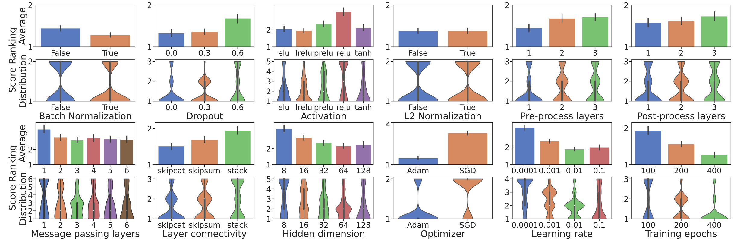
Our design space covers over 40M combinations, and a full grid search will cost too much. We adapt controlled random search from GraphGym (You et al., 2020) setting the number of random experiments to 264, except that we ensure that every combination of dataset, model family, and micro-aggregation receives 2 hits. We draw bar plots and violin plots of rankings of each design choice following the same practice as GraphGym. As shown in Figure 4, in each subplot, rankings of each design choice are aggregated over all 264 setups via bar plot and violin plot. The bar plot shows the average ranking across all the 264 setups (lower is better). The violin plot indicates the smoothed distribution of the ranking of each design choice over all the 264 setups.
5.3. Evaluation of Design Dimensions Common with GraphGym
5.3.1. Overall Evaluation
The evaluation results of design dimensions common with GraphGym (You et al., 2020) are shown in Figure 4, from which we draw the following conclusions.
Findings aligned with GraphGym:
- •
-
•
There is no definitive conclusion for the best number of message passing layers; each dataset has its own best number, the same as what GraphGym observed.
-
•
The characteristic of training settings (e.g., optimizer and training epochs) is similar to GraphGym.
Findings different from GraphGym:
-
•
A single linear transformation (pre-process layer) is usually enough. We think that this is because our heterogeneous linear transformation is node type-specific which has enough parameters to transform representations.
-
•
The widely used activation Relu may no longer be as suitable in HGNNs. Tanh, LeakyReLU, and ELU are better alternatives. PReLU, stood out in GraphGym, is not the best choice in our design space.
-
•
Different from GraphGym, we found that Dropout is necessary to get better performance. We think the reason is that parameters specific to node types and relation types lead to over-parametrization.
5.3.2. Task-wise Evaluation
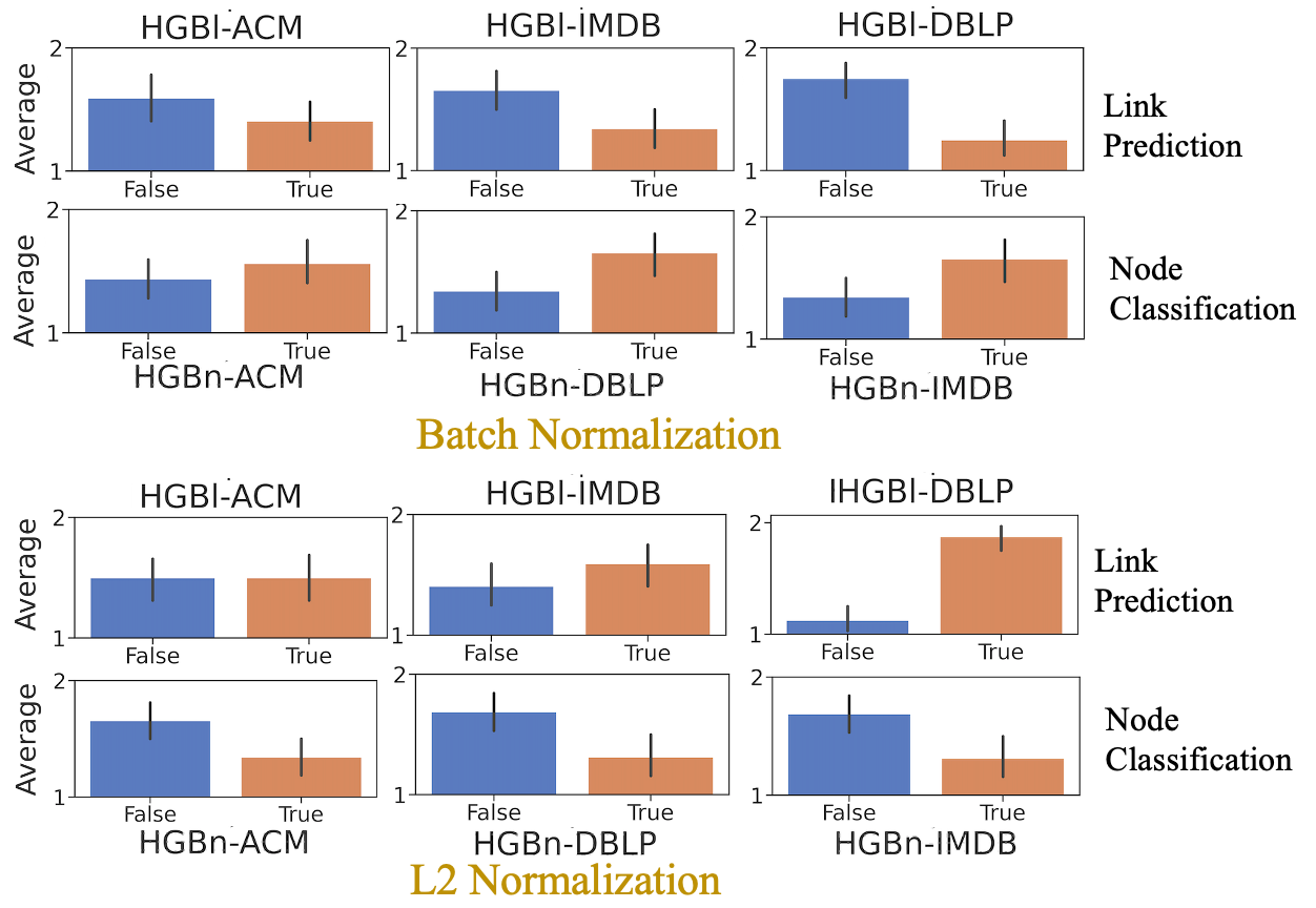
We previously observed that BN yields better performance in general. However, task-wise evaluation in Figure 5 showed that BN is better on link prediction but worse on node classification. Meanwhile, although L2-Norm does not seem to help in overall performance, it actually performs better on node classification but worse on link prediction. We think that BN scales and shifts nodes according to the global information, which may lead to more similar representations and damage the performance of the node classification task, and L2-Norm scales the representation and thus the link score to [-1,1], which may invalidate the Sigmoid of the score function.
5.4. Evaluation of Unique Design Dimensions in HGNNs
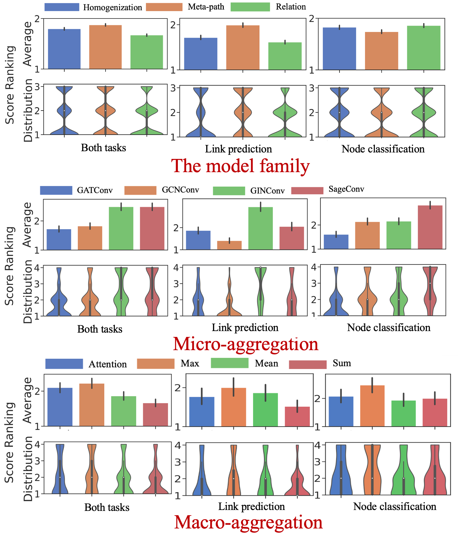
How to design and apply HGNN is our core issue. This section analyzes unique design dimensions in HGNNs to describe the characteristics of high-level architecture designs. From the average ranking shown in Figure 6, we can see that the meta-path model family has a small advantage in the node classification task. The relation model family outperforms in aggregated results in all datasets, and the homogenization model family is competitive. For the micro-aggregation design dimension, GCNConv and GATConv are preferable for link prediction task and node classification task, respectively. For the macro-aggregation design dimension, Mean and Sum have a more significant advantage.
5.4.1. The Model Family
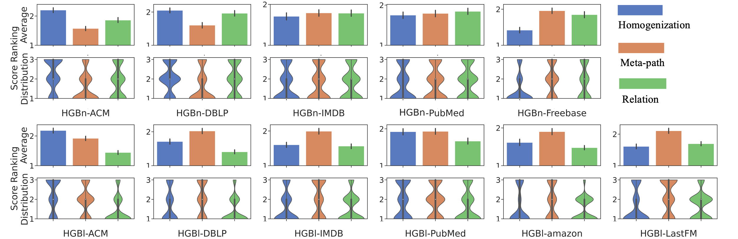
To more comprehensively describe the corresponding characteristics of different model families, we analyze the results across datasets as shown in Figure 7 and highlight some findings below.
The meta-path model family helps node classification. In node classification task, the meta-path model family outperforms visibly than the other model families on datasets HGBn-ACM and HGBn-DBLP, where we think some informative and effective meta-paths have been empirically discovered. Some experimental analysis for meta-paths can be found in Appendix D.1.
The meta-path model family does not help link prediction. In previous works, few variants of the meta-path model family were applied to the link prediction task. Although our unified framework can apply the meta-path model family to the link prediction task, the meta-path model family does not perform well on all datasets of link prediction as shown in Figure 7. We think this is because the information from the edges in the original graph is important in link prediction, and the meta-path model family ignores it.
The relation model family is a safer choice in all datasets. From Figure 7, the relation model family stands out in link prediction task, which confirms the necessity to preserve the edges as well as their type information in the original graph. Compared with the homogenization model family, the relation model family has more trainable parameters which have a linear relationship with the number of edge types. Surprisingly, the relation model family is not very effective in HGBl-Freebase with much heterogeneity, which has 8 node types and 36 edge types. We think that too many parameters lead to over-fitting, which may challenge the relation model family. According to the distribution of ranking, the relation model family has a significantly lower probability of being ranked last. Therefore, the relation model family is a safer choice.
The homogenization model family with the least trainable parameters is still competitive. As shown in Figure 7, the homogenization model family is still competitive against the relation model family on HGBl-IMDB, and even outperforms the latter on HGBn-Freebase and HGBl-LastFM. Therefore, the homogenization model family is not negligible as a baseline even on heterogeneous graphs, which aligned with (Lv et al., 2021).
5.4.2. The Micro-aggregation and the Macro-aggregation Design Dimensions
The existing HGNNs are usually inspired by GNNs and apply different micro-aggregation (e.g., GCNConv, GATConv). The micro-aggregation design dimension in our design space brings many variants to the existing HGNNs. As shown in Figure 6, the results of comparison between micro-aggregation vary greatly across tasks. We provide ranking analysis on different datasets in Appendix D.2.
For the macro-aggregation design dimension, Figure 6 shows that Sum has a great advantage in both tasks, which is aligned with the theory that Sum aggregation is theoretically most expressive (Xu et al., 2019). Surprisingly, Attention is not so effective as Sum, and we think the micro-aggregation is powerful enough, resulting that complicated Attention in macro-aggregation is not necessary.
| Design Dimension | Our Condensed Design Space | Condensed Design Space in GraphGym |
| Batch Normalization | True, False | True |
| Dropout | 0, 0.3 | 0 |
| Activation | ELU LeakyReLU Tanh | PReLU |
| L2 Normalization | True, False | - |
| Layer Connectivity | SKIP-SUM, SKIP-CAT | SKIP-SUM, SKIP-CAT |
| Pre-process Layers | 1 | 1, 2 |
| Message Passing Layers | 1, 2, 3, 4, 5, 6 | 2, 4, 6, 8 |
| Post-process Layers | 1, 2 | 2, 3 |
| Optimizer | Adam | Adam |
| Learning Rate | 0.1, 0.01 | 0.01 |
| Training Epochs | 400 | 400 |
| Hidden dimension | 64, 128 | - |
| HGBn-DBLP | HGBn-ACM | HGBl-amazon | HGBl-LastFM | ||||||
| Macro-F1 | Micro-F1 | Macro-F1 | Micro-F1 | ROC-AUC | MRR | ROC-AUC | MRR | Average Rank | |
| GCN | 90.84 | 91.47 | 92.17 | 92.12 | 92.84 | 97.050.12 | 59.17 | 79.38 | 3.75 |
| GAT | 93.83 | 93.39 | 92.26 | 92.19 | 91.65 | 96.58 | 58.56 | 77.04 | 3.63 |
| RGCN | 91.52 | 92.07 | 91.55 | 91.41 | 86.34 | 93.92 | 57.21 | 77.68 | 5.13 |
| HAN | 91.67 | 92.05 | 90.89 | 90.79 | - | - | - | - | 6.63 |
| HGT | 93.01 | 93.49 | 91.12 | 91.00 | 88.26 | 93.87 | 54.99 | 74.96 | 5.25 |
| Simple-HGN | 94.01 | 94.46 | 93.420.44 | 93.350.45 | 93.49 | 96.94 | 67.59 | 90.81 | 1.75 |
| Ours | 94.240.42 | 94.630.40 | 92.50 0.14 | 92.380.10 | 95.150.43 | 96.56 | 70.150.77 | 91.120.38 | 1.63 |
| Dataset | Model Family | Micro- aggregation | Macro- aggregation | BN | L2-Norm | Dropout | Activation | Layer Connectivity | Message Passing Layers | Post- process Layers |
| HGBn-ACM | Relation | GCNConv | Sum | False | True | 0.0 | Tanh | SKIP-SUM | 2 | 2 |
| HGBn-DBLP | Homogenization | GATConv | - | True | True | 0.0 | LeakyRelu | SKIP-SUM | 3 | 2 |
| HGBl-amazon | Meta-path | GATConv | Attention | True | False | 0.0 | LeakyRelu | SKIP-SUM | 5 | 1 |
| HGBl-LastFM | Homogenization | SageConv | - | True | False | 0.3 | Elu | SKIP-CAT | 5 | 2 |
5.5. Evaluation of Condensed Design Space
Above experiments reveals that it is hard to design a single HGNN model that can guarantee outstanding performance across diverse scenarios in the real world. According to the findings in Section 5.3.1, we condensed the design space to facilitate model searching. Specifically, we remove some bad choices in design dimensions and retain some essential design dimensions (e.g., high-level architectural structures and helpful design principles). The evaluation of HGB shows that a simple random search in the condensed design space can find the best designs. More experimental results compared GraphGym (You et al., 2020) and GraphNAS (Gao et al., 2019) are analyzed in Appendix E.
5.5.1. The Condensed Design Space
For common design dimensions with GraphGym, Table 7 compares the condensed design spaces we and GraphGym proposed. We retain some of the design dimensions same as GraphGym if the findings in Section 5.3.1 are aligned (i.e., layer connectivity, optimizer, and training epochs). We propose our own choices for the different dimensions in conclusion (e.g., Dropout, activation, BN, L2-Norm, etc.). For unique design dimensions in HGNN, we conclude that the micro-aggregation and model family design dimensions vary greatly across datasets or tasks. So we retain all choices in unique design dimensions and aim to find out whether the variants of existing HGNNs could gain improvements in HGB.
The original design space contains over 40M combinations, and the condensed design space contains 70K combinations. So the possible combination of the design dimensions in condensed design space is reduced by nearly 500 times.
5.5.2. Evaluation in Heterogeneous Graph Benchmark (HGB)
To compare with the performance of the standard HGNNs, we evaluate our condensed design space in a new benchmark HGB. We randomly searched 100 designs from condensed design space and evaluated the best design of validation set in HGB. As shown in Table 8, our designs with condensed design space can achieve comparable performance. So we can easily achieve SOTA performance with a simple random search in the condensed design space. Table 9 shows the best designs we found in our condensed design space, which cover the variants of RGCN and HAN. It also confirms that the meta-path model family and the relation model family have great performance in HGB and answers the question “are meta-path or variants still useful in GNNs?” from (Lv et al., 2021). Note that this result does not contradict the conclusion from (Lv et al., 2021), as our design space includes much more components than the vanilla RGCN or HAN model, and proper components can make up shortcomings of an existing model.
6. Conclusion and Discussion
In this work, we propose a unified framework of HGNN and define a design space for HGNN, which offers us a module-level sight to evaluate HGNN models. Specifically, we comprehensively analyze the common design dimensions with GraphGym and the unique design dimensions in HGNN. After that, we distill some findings and condense the original design space. Finally, experimental results show that our condensed design space outperforms others, and gains the best average ranking in a benchmark HGB. With that, we demonstrate that focusing on the design space could help drive advances in HGNN research.
How to condense the design space? In our work, the condensed design space is distilled according to the findings within extensive experiments, which still needs much effort and intuitive experience. A recently proposed work KGTuner (Zhang et al., 2022), which analyzed the design space for knowledge graph embedding, proposed a more systematic way to shrink and decouple the search space, which can be a potential improvement of this work
Acknowledgements.
This work is supported in part by the National Natural Science Foundation of China (No. U20B2045, 62192784, 62002029, 62172052, 61772082).References
- (1)
- Bi et al. (2020) Ye Bi, Liqiang Song, Mengqiu Yao, Zhenyu Wu, Jianming Wang, and Jing Xiao. 2020. A heterogeneous information network based cross domain insurance recommendation system for cold start users. In SIGIR. 2211–2220.
- Cao et al. (2021) Xianshuai Cao, Yuliang Shi, Han Yu, Jihu Wang, Xinjun Wang, Zhongmin Yan, and Zhiyong Chen. 2021. DEKR: Description Enhanced Knowledge Graph for Machine Learning Method Recommendation. In SIGIR. 203–212.
- Chang et al. (2020) Jianxin Chang, Chen Gao, Xiangnan He, Depeng Jin, and Yong Li. 2020. Bundle recommendation with graph convolutional networks. In SIGIR. 1673–1676.
- Chang et al. (2021) Jianxin Chang, Chen Gao, Yu Zheng, Yiqun Hui, Yanan Niu, Yang Song, Depeng Jin, and Yong Li. 2021. Sequential recommendation with graph neural networks. In SIGIR. 378–387.
- Chen et al. (2021a) Chong Chen, Weizhi Ma, Min Zhang, Zhaowei Wang, Xiuqiang He, Chenyang Wang, Yiqun Liu, and Shaoping Ma. 2021a. Graph Heterogeneous Multi-Relational Recommendation. In AAAI, Vol. 35. 3958–3966.
- Chen et al. (2021b) Huiyuan Chen, Lan Wang, Yusan Lin, Chin-Chia Michael Yeh, Fei Wang, and Hao Yang. 2021b. Structured graph convolutional networks with stochastic masks for recommender systems. In SIGIR. 614–623.
- Dacrema et al. (2019) Maurizio Ferrari Dacrema, Paolo Cremonesi, and Dietmar Jannach. 2019. Are we really making much progress? A worrying analysis of recent neural recommendation approaches. In RecSys. 101–109.
- Ding et al. (2021) Yuhui Ding, Quanming Yao, Huan Zhao, and Tong Zhang. 2021. DiffMG: Differentiable Meta Graph Search for Heterogeneous Graph Neural Networks. In KDD.
- Dwivedi et al. (2020) Vijay Prakash Dwivedi, Chaitanya K Joshi, Thomas Laurent, Yoshua Bengio, and Xavier Bresson. 2020. Benchmarking graph neural networks. arXiv preprint arXiv:2003.00982 (2020).
- Errica et al. (2020) Federico Errica, Marco Podda, Davide Bacciu, and Alessio Micheli. 2020. A Fair Comparison of Graph Neural Networks for Graph Classification. In ICLR.
- Fan et al. (2019) Wenqi Fan, Yao Ma, Qing Li, Yuan He, Eric Zhao, Jiliang Tang, and Dawei Yin. 2019. Graph neural networks for social recommendation. In WWW. 417–426.
- Fang et al. (2019) Yang Fang, Xiang Zhao, Peixin Huang, Weidong Xiao, and Maarten de Rijke. 2019. M-HIN: complex embeddings for heterogeneous information networks via metagraphs. In SIGIR. 913–916.
- Fu et al. (2020) Xinyu Fu, Jiani Zhang, Ziqiao Meng, and Irwin King. 2020. Magnn: Metapath aggregated graph neural network for heterogeneous graph embedding. In WWW. 2331–2341.
- Gao et al. (2019) Yang Gao, Hong Yang, Peng Zhang, Chuan Zhou, and Yue Hu. 2019. Graphnas: Graph neural architecture search with reinforcement learning. arXiv preprint arXiv:1904.09981 (2019).
- Ghazimatin (2020) Azin Ghazimatin. 2020. Explaining Recommendations in Heterogeneous Networks. In SIGIR. 2479–2479.
- Gilmer et al. (2017) Justin Gilmer, Samuel S Schoenholz, Patrick F Riley, Oriol Vinyals, and George E Dahl. 2017. Neural message passing for quantum chemistry. In ICML. 1263–1272.
- Gong et al. (2020) Jibing Gong, Shen Wang, Jinlong Wang, Wenzheng Feng, Hao Peng, Jie Tang, and Philip S Yu. 2020. Attentional graph convolutional networks for knowledge concept recommendation in moocs in a heterogeneous view. In SIGIR. 79–88.
- Guo and Liu (2015) Chun Guo and Xiaozhong Liu. 2015. Automatic feature generation on heterogeneous graph for music recommendation. In SIGIR. 807–810.
- Hamilton et al. (2017) William L Hamilton, Rex Ying, and Jure Leskovec. 2017. Inductive representation learning on large graphs. In NeurIPS. 1025–1035.
- Hao et al. (2020) Xiaorong Hao, Tao Lian, and Li Wang. 2020. Dynamic link prediction by integrating node vector evolution and local neighborhood representation. In SIGIR. 1717–1720.
- He et al. (2016) Kaiming He, Xiangyu Zhang, Shaoqing Ren, and Jian Sun. 2016. Deep residual learning for image recognition. In CVPR. 770–778.
- Hong et al. (2020) Huiting Hong, Hantao Guo, Yucheng Lin, Xiaoqing Yang, Zang Li, and Jieping Ye. 2020. An attention-based graph neural network for heterogeneous structural learning. In AAAI, Vol. 34. 4132–4139.
- Hu et al. (2019) Binbin Hu, Zhiqiang Zhang, Chuan Shi, Jun Zhou, Xiaolong Li, and Yuan Qi. 2019. Cash-out user detection based on attributed heterogeneous information network with a hierarchical attention mechanism. In AAAI, Vol. 33. 946–953.
- Hu et al. (2020) Ziniu Hu, Yuxiao Dong, Kuansan Wang, and Yizhou Sun. 2020. Heterogeneous graph transformer. In WWW. 2704–2710.
- Huang et al. (2017) Gao Huang, Zhuang Liu, Laurens Van Der Maaten, and Kilian Q Weinberger. 2017. Densely connected convolutional networks. In CVPR. 4700–4708.
- Ioffe and Szegedy (2015) Sergey Ioffe and Christian Szegedy. 2015. Batch normalization: Accelerating deep network training by reducing internal covariate shift. In ICML. PMLR, 448–456.
- Ji et al. (2021a) Houye Ji, Xiao Wang, Chuan Shi, Bai Wang, and Philip Yu. 2021a. Heterogeneous Graph Propagation Network. TKDE (2021).
- Ji et al. (2021b) Houye Ji, Junxiong Zhu, Chuan Shi, Xiao Wang, Bai Wang, Chaoyu Zhang, Zixuan Zhu, Feng Zhang, and Yanghua Li. 2021b. Large-scale Comb-K Recommendation. In WWW. 2512–2523.
- Jiang et al. (2018) Zhuoren Jiang, Yue Yin, Liangcai Gao, Yao Lu, and Xiaozhong Liu. 2018. Cross-language citation recommendation via hierarchical representation learning on heterogeneous graph. In SIGIR. 635–644.
- Jin et al. (2020) Jiarui Jin, Kounianhua Du, Weinan Zhang, Jiarui Qin, Yuchen Fang, Yong Yu, Zheng Zhang, and Alexander J Smola. 2020. Learning Interaction Models of Structured Neighborhood on Heterogeneous Information Network. arXiv preprint arXiv:2011.12683 (2020).
- Kipf and Welling (2017) Thomas N. Kipf and Max Welling. 2017. Semi-Supervised Classification with Graph Convolutional Networks. (2017).
- Li et al. (2019) Guohao Li, Matthias Müller, Ali Thabet, and Bernard Ghanem. 2019. DeepGCNs: Can GCNs Go as Deep as CNNs?. In ICCV.
- Li et al. (2020) Zekun Li, Yujia Zheng, Shu Wu, Xiaoyu Zhang, and Liang Wang. 2020. Heterogeneous Graph Collaborative Filtering. arXiv preprint arXiv:2011.06807 (2020).
- Linmei et al. (2019) Hu Linmei, Tianchi Yang, Chuan Shi, Houye Ji, and Xiaoli Li. 2019. Heterogeneous graph attention networks for semi-supervised short text classification. In EMNLP-IJCNLP. 4821–4830.
- Liu et al. (2020) Siwei Liu, Iadh Ounis, Craig Macdonald, and Zaiqiao Meng. 2020. A heterogeneous graph neural model for cold-start recommendation. In SIGIR. 2029–2032.
- Lv et al. (2021) Qingsong Lv, Ming Ding, Qiang Liu, Yuxiang Chen, Wenzheng Feng, Siming He, Chang Zhou, Jianguo Jiang, Yuxiao Dong, and Jie Tang. 2021. Are we really making much progress? Revisiting, benchmarking and refining heterogeneous graph neural networks. In KDD. 1150–1160.
- Mei et al. (2018) Jiajie Mei, Richong Zhang, Yongyi Mao, and Ting Deng. 2018. On link prediction in knowledge bases: Max-K criterion and prediction protocols. In SIGIR. 755–764.
- Pei et al. (2019) Hongbin Pei, Bingzhe Wei, Kevin Chen-Chuan Chang, Yu Lei, and Bo Yang. 2019. Geom-GCN: Geometric Graph Convolutional Networks. In ICLR.
- Radosavovic et al. (2019) Ilija Radosavovic, Justin Johnson, Saining Xie, Wan-Yen Lo, and Piotr Dollár. 2019. On network design spaces for visual recognition. In ICCV. 1882–1890.
- Radosavovic et al. (2020) Ilija Radosavovic, Raj Prateek Kosaraju, Ross Girshick, Kaiming He, and Piotr Dollár. 2020. Designing network design spaces. In CVPR. 10428–10436.
- Schlichtkrull et al. (2018) Michael Schlichtkrull, Thomas N Kipf, Peter Bloem, Rianne Van Den Berg, Ivan Titov, and Max Welling. 2018. Modeling relational data with graph convolutional networks. In ESWC. Springer, 593–607.
- Shchur et al. (2018) Oleksandr Shchur, Maximilian Mumme, Aleksandar Bojchevski, and Stephan Günnemann. 2018. Pitfalls of graph neural network evaluation. arXiv preprint arXiv:1811.05868 (2018).
- Srivastava et al. (2014) Nitish Srivastava, Geoffrey Hinton, Alex Krizhevsky, Ilya Sutskever, and Ruslan Salakhutdinov. 2014. Dropout: a simple way to prevent neural networks from overfitting. The journal of machine learning research 15, 1 (2014), 1929–1958.
- Sun et al. (2020) Xiaoqing Sun, Jiahai Yang, Zhiliang Wang, and Heng Liu. 2020. Hgdom: Heterogeneous graph convolutional networks for malicious domain detection. In NOMS. IEEE, 1–9.
- Sun et al. (2011) Yizhou Sun, Jiawei Han, Xifeng Yan, Philip S Yu, and Tianyi Wu. 2011. Pathsim: Meta path-based top-k similarity search in heterogeneous information networks. PVLDB 4, 11 (2011), 992–1003.
- Tang et al. (2008) Jie Tang, Jing Zhang, Limin Yao, Juanzi Li, Li Zhang, and Zhong Su. 2008. Arnetminer: extraction and mining of academic social networks. In KDD. 990–998.
- Veličković et al. (2018) Petar Veličković, Guillem Cucurull, Arantxa Casanova, Adriana Romero, Pietro Liò, and Yoshua Bengio. 2018. Graph Attention Networks. In ICLR.
- Wang et al. (2019c) Weiqing Wang, Hongzhi Yin, Xingzhong Du, Wen Hua, Yongjun Li, and Quoc Viet Hung Nguyen. 2019c. Online user representation learning across heterogeneous social networks. In SIGIRl. 545–554.
- Wang et al. (2020) Xiao Wang, Deyu Bo, Chuan Shi, Shaohua Fan, Yanfang Ye, and Philip S Yu. 2020. A Survey on Heterogeneous Graph Embedding: Methods. Techniques, Applications and Sources (2020).
- Wang et al. (2019a) Xiang Wang, Xiangnan He, Meng Wang, Fuli Feng, and Tat-Seng Chua. 2019a. Neural graph collaborative filtering. In SIGIR. 165–174.
- Wang et al. (2019b) Xiao Wang, Houye Ji, Chuan Shi, Bai Wang, Yanfang Ye, Peng Cui, and Philip S Yu. 2019b. Heterogeneous graph attention network. In WWW. 2022–2032.
- Wang et al. (2022) Zhenyi Wang, Huan Zhao, and Chuan Shi. 2022. Profiling the Design Space for Graph Neural Networks Based Collaborative Filtering. In WSDM. 1109–1119.
- Xu et al. (2019) Keyulu Xu, Weihua Hu, Jure Leskovec, and Stefanie Jegelka. 2019. How Powerful are Graph Neural Networks?. In ICLR.
- Xu et al. (2018) Keyulu Xu, Chengtao Li, Yonglong Tian, Tomohiro Sonobe, Ken-ichi Kawarabayashi, and Stefanie Jegelka. 2018. Representation learning on graphs with jumping knowledge networks. In ICML. PMLR, 5453–5462.
- You et al. (2020) Jiaxuan You, Zhitao Ying, and Jure Leskovec. 2020. Design space for graph neural networks. NeurIPS 33 (2020).
- Yu et al. (2020) Le Yu, Leilei Sun, Bowen Du, Chuanren Liu, Weifeng Lv, and Hui Xiong. 2020. Hybrid Micro/Macro Level Convolution for Heterogeneous Graph Learning. arXiv preprint arXiv:2012.14722 (2020).
- Yu et al. (2021) Tan Yu, Yi Yang, Yi Li, Lin Liu, Hongliang Fei, and Ping Li. 2021. Heterogeneous attention network for effective and efficient cross-modal retrieval. In SIGIR. 1146–1156.
- Yun et al. (2019) Seongjun Yun, Minbyul Jeong, Raehyun Kim, Jaewoo Kang, and Hyunwoo J Kim. 2019. Graph transformer networks. NeurIPS 32 (2019), 11983–11993.
- Zhang et al. (2022) Yongqi Zhang, Zhanke Zhou, Quanming Yao, and Yong Li. 2022. KGTuner: Efficient Hyper-parameter Search for Knowledge Graph Learning. In ACL.
- Zhao et al. (2017) Huan Zhao, Quanming Yao, Jianda Li, Yangqiu Song, and Dik Lun Lee. 2017. Meta-graph based recommendation fusion over heterogeneous information networks. In KDD. 635–644.
- Zhao et al. (2019) Jun Zhao, Zhou Zhou, Ziyu Guan, Wei Zhao, Wei Ning, Guang Qiu, and Xiaofei He. 2019. Intentgc: a scalable graph convolution framework fusing heterogeneous information for recommendation. In KDD. 2347–2357.
Appendix A Preliminary
A.1. Graph Neural Network
Graph Neural Networks (GNNs) aim to apply deep neural networks to graph-structured data. Here we focus on message passing GNNs which could be implemented efficiently and proven great performance.
Definition A.0 (Message Passing GNNs (Gilmer et al., 2017)).
Message passing GNNs aim to learn a representation vector for each node after -th message passing layers of transformation, and means the output dimension in -th message passing layer. The message passing paradigm defines the following node-wise and edge-wise computation for each layer as:
| (5) |
where means neighbors of node , is a message function defined on each edge to generate a message by combining the features of its incident nodes, and denotes an edge from node to ;
| (6) |
where means neighbors of node , is an update function defined on each node to update the node representation by aggregating its incoming messages using the aggregation function .
Example: GraphSAGE (Hamilton et al., 2017) can be formalized as a message passing GNN, where the message function is and the update function is .
A.2. Heterogeneous Graph
Definition A.0 (Heterogeneous Graph).
A heterogeneous graph, denoted as , consists of a node set and an edge set . A heterogeneous graph is also associated with a node type mapping function and an edge type (or relation type) mapping function . and denote the sets of node types and edge types. Each node has one node type . Similarly, for an edge from node to node , . When or , it is a heterogeneous graph, otherwise it is a homogeneous graph.
Example. As shown in Figure 1 (left), we construct a simple heterogeneous graph to show an academic network. It consists of multiple types of objects (Paper(P), Author (A), Conference(C)) and relations (written-relation between papers and authors, published-relation between papers and conferences).
Definition A.0 (Relation Subgraph).
A heterogeneous graph can also be represented by a set of adjacency matrices , where is the number of edge types . is an adjacency matrix where is non-zero when there is an edge with -th type from node to node . and are numbers of source and target nodes corresponding to the edge type respectively. A relation subgraph of -th edge type is therefore a subgraph whose adjacency matrix is . As shown in Figure 2 (b), the underlying data structure of the academic network in Figure 1 (left) consists of four adjacency matrices.
Definition A.0 (Meta-path (Sun et al., 2011)).
A meta-path is defined as a path in the form of which describes a composite relation between two nodes and , where denotes the -th relation type of meta-path and denotes the composition operator on relations.
Definition A.0 (Meta-path Subgraph).
Given a meta-path , , the adjacency matrix can be obtained by a multiplication of adjacency matrices according relations as
| (7) |
The notion of meta-path subsumes multi-hop connections and a meta-path subgraph is multiple relation subgraphs matrices multiplication shown in Figure 2 (b) (iii). So relation subgraph is a special case of meta-path subgraph which is only composited by a relation subgraph. When meta-path beginning node type and ending node type are the same, meta-path subgraph is a homogeneous graph, otherwise a bipartite graph.
Appendix B Design Space
B.1. Common Design with GraphGym
Intra-layer
Same with GNNs, an HGNN contains several Heterogeneous GNN layers, where each layer could have diverse design dimensions. As illustrated in Figure 3, the adopted Heterogeneous GNN layer has an aggregation layer which involves unique design dimensions discussed later, followed by a sequence of modules: (1) batch normalization BN() (Ioffe and Szegedy, 2015); (2) dropout DROP() (Srivastava et al., 2014); (3) nonlinear activation function ACT(); (4) L2 Normalization L2-Norm(). Formally, the L-th heterogeneous GNN layer can be defined as:
| (8) |
Inter-layer
The layers of message passing, pre-processor and post-processor are supposed to be considered, which are essential design dimensions according to empirical evidence from neural networks. HGNNs face the problems of vanishing gradient, over-fitting and over-smoothing, and the last problem is seen as the obstacles to stack deeper GNN layers. Inspired by ResNet (He et al., 2016) to alleviate the problems, skip connection (Li et al., 2019; Xu et al., 2018) has been proven to significant effect. Therefore, we investigate two choices of skip connections: SKIP-SUM (He et al., 2016) and SKIP-CAT (Huang et al., 2017) with STACK as a basic comparison.
Training Settings
As a part of deep learning, we also want to analyze design dimensions on training settings, like optimizer, learning rate and training epochs. Besides, the hidden dimension is also included here involving the trainable parameters.
| Dataset | #Nodes | #Node Types | #Edges | #Edge Types | Name for Node Classification Task | Target Node | #Classes | Name for Link Prediction Task | Target Link for Link Prediction |
| DBLP | 26,128 | 4 | 239,566 | 6 | HGBn-DBLP | author | 4 | HGBl-DBLP | author-paper |
| IMDB | 21,420 | 4 | 86,642 | 6 | HGBn-IMDB | movie | 5 | HGBl-IMDB | actor-movie |
| ACM | 10,942 | 4 | 547,872 | 8 | HGBn-ACM | paper | 3 | HGBl-ACM | paper-paper |
| Freebase | 180,098 | 8 | 1,057,688 | 36 | HGBn-Freebase | book | 7 | - | - |
| PubMed | 63,109 | 4 | 244,986 | 10 | HGBn-PubMed | disease | 8 | HGBl-PubMed | disease-disease |
| Amazon | 10,099 | 1 | 148,659 | 2 | - | - | - | HGBl-amazon | product-product |
| LastFM | 20,612 | 3 | 141,521 | 3 | - | - | - | HGBl-LastFM | user-artist |
Appendix C Dataset
We select datasets from the Heterogeneous Graph Benchmark (HGB) (Lv et al., 2021), a benchmark with multiple datasets of various heterogeneity (i.e., the number of nodes and edge types), for node classification and link prediction tasks. The HGB is organized as a public competition, so it does not release the test label to prevent data leakage. Since formal submission to the public leaderboard costs a large amount of time and submission resources, we only report the test performance of the configuration with the best validation performance in Table 8, using the same metrics as in (Lv et al., 2021). Other experiments are evaluated on a validation set with three random 80-20 training-validation splits. The statistics of HGB are shown in Table 10. We select five datasets (DBLP, IMDB, ACM, Freebase, PubMed) for node classification task, six datasets (DBLP, IMDB, ACM, amazon, LastFM, PubMed) for link prediction task.
Appendix D Evaluation of Unique Design Dimensions
D.1. Analysis for Meta-path
| Dataset | Meaning | Meta-path | |
| HGBn-ACM | P: paper A: author S: subject c: citation relation r: reference relation | PrP | 0.4991 |
| PcP | 0.4927 | ||
| PAP | 0.6511 | ||
| PSP | 0.4572 | ||
| PcPAP | 0.5012 | ||
| PcPSP | 0.4305 | ||
| PrPAP | 0.4841 | ||
| PrPSP | 0.4204 | ||
| HGBn-DBLP | A: author P: paper T: term V: venue | APA | 0.7564 |
| APTPA | 0.2876 | ||
| APVPA | 0.3896 | ||
| HGBn-PubMed | D: disease G: gene C: chemical S: species | DD | 0.0169 |
| DCD | 0.1997 | ||
| DDD | 0.1945 | ||
| DGD | 0.2567 | ||
| DSD | 0.2477 | ||
| HGBn-Freebase | B: book F: film L: location M: music P: person S: sport O: organization U: business | BB | 0.1733 |
| BUB | 0.0889 | ||
| BFB | 0.1033 | ||
| BLMB | 0.0303 | ||
| BOFB | 0.3341 | ||
| BPB | 0.1928 | ||
| BPSB | 0.0603 |
In node classification task, the meta-path model family outperforms visibly than the other model families on datasets HGBn-ACM and HGBn-DBLP, where we think some informative and effective meta-paths have been empirically discovered. The micro-aggregation modules are MPNN networks that tend to learn similar representations for proximal nodes in a graph (Pei et al., 2019). Moreover, the meta-path model family aims to bring nodes with the same type topologically closer with meta-path subgraph extraction, hoping that the extracted subgraph is assortative (e.g., citation networks) where node homophily holds (i.e., nodes with the same label tend to be proximal, and vice versa). Based on that, we measure the homophily (Pei et al., 2019) in subgraphs extracted by meta-path , which is defined as
| (9) |
where and represent the label of node and , respectively.
As shown in Table 11, the homophily of homogeneous subgraphs extracted by predefined meta-path in HGBn-ACM and HGBn-DBLP is significantly higher than that in HGBn-PubMed and HGBn-Freebase. For node classification task, the homophily of subgraphs extracted by meta-paths may be a helpful reference for meta-path selection. So for the question “are meta-path or variants still useful in GNNs?” from (Lv et al., 2021), we think that the meta-path model family is still useful with well-defined meta-paths that reveal task-specific semantics.
D.2. Analysis for Micro-aggregation
As shown in Figure 8, the results of comparison between micro-aggregation vary greatly across datasets. The GCNConv has gained significant advantages on datasets HGBl-amazon and HGBl-LastFM. The GATConv performs best on the two datasets. The SOTA model GINConv for graph-level tasks can also stand out in one dataset HGBn-DBLP here. It confirms that there is no single GNN model can perform well in all situations.
Appendix E Evaluation of condensed design space
E.1. Evaluation of Different Design Spaces
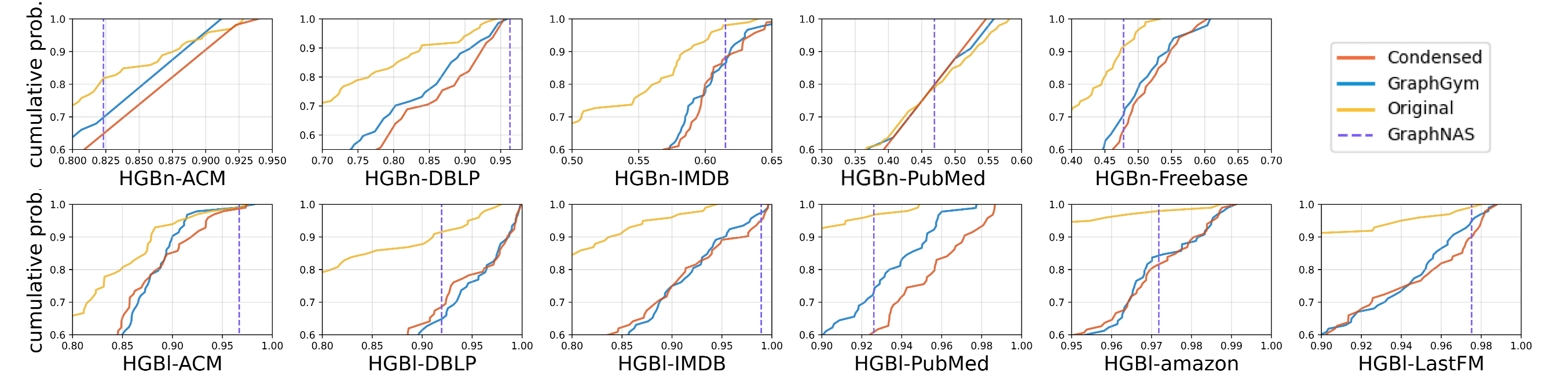
Plotting ranking with controlled random search can only work in the same design space, and is not suitable for evaluation across different design spaces. Therefore, we plot for each design space the empirical distribution function (EDF) (Radosavovic et al., 2019): given configurations and their respective scores , EDF is defined as
| (10) |
EDF essentially tells the probability of a random hyperparameter configuration that cannot achieve a given performance metric. Therefore, with -axis being the performance metric and -axis being the probability, an EDF curve closer to the lower-right corner indicates that a random configuration is more likely to get a better result.
Though the condensed design space in GraphGym is small enough to perform a full grid search for GNNs, it is not so much suitable for HGNNs due to more complicated HGNN models. To verify the effectiveness of our condensed design space, we compare it with the original design space and the condensed design from GraphGym (You et al., 2020). We randomly search 100 designs in three spaces, respectively.
As shown in Figure 9, our condensed design space outperforms the others. Specifically, the original design space has many bad choices (i.e., optimizer with SGD) and performs worst in the distribution estimates. On the other hand, the best design in the original design space is competitive, but at a much higher search cost. Besides, the better performance in our condensed design space compared with GraphGym shows that we cannot simply transfer the design space condensed from homogeneous graphs to HGNNs, and specific condensation is required.
E.2. Comparison with GraphNAS
We also apply a GNN neural architecture search method GraphNAS (Gao et al., 2019) in the original design space as a comparison. The NAS is to find the best architecture, so we only report the best performance of GraphNAS in Figure 9. Though GraphNAS outperforms in HGBn-DBLP and gains excellent performance in HGBl-ACM and HGBl-IMDB, it performs worst in other datasets. So compared with GraphNAS, our design space has more significant advantages in robustness and stability. We think that we need a more advanced NAS method (i.e., DiffMG (Ding et al., 2021)) for our design space in future work.