Colored HOMFLY-PT polynomials of quasi-alternating $3$-braid knots

Abstract

Obtaining a closed form expression for the colored HOMFLY-PT polynomials of knots from $3$-strand braids carrying arbitrary $SU(N)$ representation is a challenging problem. In this paper, we confine our interest to twisted generalized hybrid weaving knots which we denote hereafter by $\hat{Q}_{3}(m_{1},-m_{2},n,\ell)$. This family of knots not only generalizes the well-known class of weaving knots but also contains an infinite family of quasi-alternating knots. Interestingly, we obtain a closed form expression for the HOMFLY-PT polynomial of $\hat{Q}_{3}(m_{1},-m_{2},n,\ell)$ using a modified version of the Reshitikhin-Turaev method. In addition, we compute the exact coefficients of the Jones polynomials and the Alexander polynomials of quasi-alternating knots $\hat{Q}_{3}(1,-1,n,\pm 1)$. For these homologically-thin knots, such coefficients are known to be the ranks of their Khovanov and link Floer homologies, respectively. We also show that the asymptotic behaviour of the coefficients of the Alexander polynomial is trapezoidal. On the other hand, we compute the $[r]$-colored HOMFLY-PT polynomials of quasi alternating knots for small values of $r$. Remarkably, the study of the determinants of certain twisted weaving knots leads to establish a connection with enumerative geometry related to $m^{th}$ Lucas numbers, denoted hereafter as $L_{m,2n}$. At the end, we verify that the reformulated invariants satisfy Ooguri-Vafa conjecture and we express certain BPS integers in terms of hyper-geometric functions ${}_{2}{\bf F}_{1}\left[\begin{matrix}a&,&b&,&c\end{matrix};z\right]$.

1 Introduction

Knot theory is the branch of low dimensional topology concerned with the study of the spatial configurations of embedded circles in the 3-dimensional space. These embeddings are considered up to natural deformations called isotopies. It is well known that the study of knots and links up to isotopies is equivalent to the study of their regular planar projections up to some local moves. A link projection is called alternating if the overpass and the underpass alternate as one travels along any component of the link. The class of alternating links is of central importance in classical knot theory and the study of the Jones polynomials of these links led to the solution of long-standing conjectures in knot theory [1]. Indeed, certain quantum invariants reflect the alternating property of the link in a very obvious way. It was also proved that these links are homologically thin in both Khovanov and link Floer homology. Moreover, the Heegaard Floer homology of the branched double cover of an alternating link $L$ depends only on the determinant of the link, ${\rm{Det}}(L)$. These interesting homological properties extend to a wider class of links called quasi-alternating links. Unlike alternating links which admit a simple diagrammatic description, quasi-alternating links are defined in the following recursive way.

Definition 1.1

The set $\mathcal{Q}$ of quasi-alternating links is the smallest set satisfying the following properties:

1. The unknot belongs to $\mathcal{Q}$.

2. If $L$ is a link with a diagram $D$ containing a crossing $c$ such that

   1. both smoothings of the diagram $D$ at the crossing $c$, $L_{0}$ and $L_{\infty}$ as in Figure 1 belong to $\mathcal{Q}$;

   2. $\det(L_{0}),\det(L_{\infty})\geq 1$;

   3. $\det(L)=\det(L_{0})+\det(L_{\infty})$;
      then $L$ is in $\mathcal{Q}$. In this case we say that $L$ is quasi-alternating with quasi-alternating diagram $D$ at the crossing $c$.

$L$                                                $L_{0}$                                                $L_{\infty}$

Figure 1: The diagram of the Link $L$ at the crossing $c$ and its smoothings $L_{0}$ and $L_{\infty}$, respecyively.

With an elementary induction on the determinant of the link, this definition can be used to prove that non-split alternating links are quasi-alternating. The knots $8_{20}$ and $8_{21}$ are the first examples, in the knot table, of non-alternating quasi-alternating knots. In general, using the definition above to decide whether a given link is quasi-alternating is a very challenging task.

For $m>1$, let $\mathcal{B}_{m}$ be the group of braids on $m$ strands. It is well known that any link in the 3-dimensional space can be represented as the closure of an $m$ braid. The smallest such integer $m$ is called the braid index of the link. Links of braid index $2$ are torus links. Links of braid index $3$ have been subject to extensive study. Indeed, braids on 3 strands have been classified, up to conjugacy, into normal forms, see [2]. This classification led to a better understanding of 3-braid links. In particular, alternating links of braid index 3 have been classified by Stoimenow [3]. Quasi-alternating links of braid index $3$ have been characterized by Baldwin [4]. Other than a finite number of links, any quasi-alternating link of braid index three is the closure of a braid of the form $\sigma_{1}^{p_{1}}\sigma_{2}^{-q_{1}}\dots\sigma_{1}^{p_{n}}\sigma_{2}^{-q_{n}}h^{\ell}$ where $p_{i},q_{i}$ are positive integers, $h$ is the central braid $(\sigma_{1}\sigma_{2})^{3}$, and $\ell=0,1,$ or $-1$. If $p_{i}=m_{1}$ for all $i$ and $q_{i}=m_{2}$ for all $i$ then this link is denoted by $\hat{Q}_{3}(m_{1},-m_{2},n,\ell)$. These links are refereed to as twisted generalized hybrid weaving knots. Note that the case $m_{1}=m_{2}=1$ and $\ell=0$, corresponds to the classical class of weaving links. If $m_{1}=m_{2}$ and $\ell=0$, then we obtain the hybrid weaving links whose colored HOMFLY-PT polynomials have been recently studied in [5]. One may easily see that these hybrid weaving links are alternating. The purpose of this paper is to extend the work in [5] to a wider class of links which in particular includes a large family of links which are quasi-alternating but not alternating. More precisely, we study the colored HOMFLY-PT polynomial of the links $\hat{Q}_{3}(m_{1},-m_{2},n,\ell)$ using a modified version of the Reshitikhin-Turaev method. Our main result is an explicit formula for the HOMFLY-PT polynomials of these class of links.

Here is an outline of the paper. In Section 2, we shall review the modified version of Reshitikhin-Turaev method for constructing knot invariants and describe the block structure form of $\mathfrak{R}$-matrices in the case of three-strand braids. In Section 3, we use the twisted trace $\Psi^{[2,1,0]}((m_{1},-m_{2},n,\ell);A,q)$, to introduce a closed form expression for the HOMFLY-PT polynomial of the knot $\hat{Q}_{3}(m_{1},m_{2},n,\ell)$. As a consequence, we show that the determinants of hybrid weaving knots are related to Lucas numbers. Further, we prove the trapezoidal behaviour of the coefficients of the Alexander polynomial of weaving knots. Section 4 is devoted to study the $[r]$-colored HOMFLY-PT polynomial of quasi-alternating knots $\hat{Q}_{3}(1,-1,n,\pm 1)$. In particular, the twisted traces of 2-dimensional matrices are expressed as Laurent polynomials $\Theta_{n,t,m,\ell}[q]$ and the colored HOMFLY-PT polynomials of quasi-alternating knots are calculated. In Section 5, we verify that the reformulated invariants from these quasi-alternating knot invariants satisfy Ooguri-Vafa Conjecture. Section 6 summarizes the paper and discusses related challenging open problems. Finally, explicit data on colored HOMFLY-PT polynomials up to representation $[r]=[4]$ as well as reformulated invariants for $\hat{Q}_{3}(1,-1,n,\pm 1)$ are given in Appendices 7, 8 and 9.

2 Knot invariants from quantum groups

A fundamental result in classical knot theory states that any link in the 3-dimensional sphere can be viewed as the closure of a braid on $m$ strands. This fact has played a key role in the development of knot theory. In particular, quantum knot invariants are constructed from representations of the braid group. Such a representation associates a quantum $\mathfrak{R}$-matrix to each of the generators of the braid group $\sigma_{1},\ldots,\sigma_{m-1}$, see [6] and [7, 8, 9]:

$$\begin{array}[]{rcl}\pi:\mathcal{B}_{m}&\rightarrow&\text{End}(V_{1}\otimes\ldots,\otimes V_{m})\\ \pi(\sigma_{\mu})&=&\mathfrak{R}_{\mu}.\end{array}$$ (1)

These matrices has to satisfy the following relations:

$${\mathfrak{R}}_{\mu}{{\mathfrak{R}}}_{\nu} = {{\mathfrak{R}}}_{\nu}{{\mathfrak{R}}}_{\mu}~{}~{}\text{for}~{}|{\mu}-{\nu}|>1~{},$$ (2)

$${{\mathfrak{R}}}_{\mu}{{\mathfrak{R}}}_{{\mu}+1}{{\mathfrak{R}}}_{{\mu}} = {{\mathfrak{R}}}_{{\mu}+1}{{\mathfrak{R}}}_{\mu}{{\mathfrak{R}}}_{{\mu}+1},~{}\text{for}~{}\ {\mu}=1,\ldots,m-2.$$ (3)

Note that the matrix $\mathfrak{R}_{\mu}$ acts on the two consecutive braid stands $\mu$ and $\mu+1$. Pictorially, $\mathfrak{R}_{\mu}$ is represented as follows:

(4)

In 1984, Jones introduced a topological invariant of oriented links through the study of representations of the braid group via certain von Neumann algebras. The Jones polynomial was later generalized to a two-variable invariant known as the HOMFLY-PT polynomial. Following the seminal work of Witten [10], colored versions of these invariants have been defined by Reshetikhin and Turaev and used to construct new quantum invariants of 3-manifolds [11, 12]. In this paper, we are interested in the so-called colored HOMFLY-PT polynomial $H_{[r]}^{\mathcal{K}}(q,A)$; a two-variable polynomial defined as follows

$$H_{[r]}^{\mathcal{K}}(q,A)={}_{q}\text{tr}_{V\otimes\dots\otimes V}\left(\,\pi(\beta_{\mathcal{K}})\,\right),$$

where ${}_{q}\text{tr}_{V}(z)$ denotes the quantum trace of $z$ [13] and $\beta_{\mathcal{K}}$ is a braid word whose closure is the knot $\mathcal{K}$. The Reshetikhin-Turaev approach, denoted hereafter RT for short, involves non-diagonal universal $\check{R}$ matrices that makes the computations of knot invariants somehow cumbersome. A more effective method is discussed in [14, 15, 16], where the colored HOMFLY-PT polynomials are viewed in the form of character decomposition. This formalism is known as the modified RT-approach. The key feature in this approach is that the braiding generators can be expressed in a block structure form. This allows a better control of the computation of knot invariants. In this article, we use modified RT-approach to compute the symmetric $[r]$-colored HOMFLY-PT polynomials for twisted generalized hybrid weaving knots.

2.1 The modified Reshetikhin-Turaev approach

In this section, we shall briefly summarize the modified RT-approach. More technical details can be found in [15, 14, 16, 17, 5]. It is worth mentioning here that we are assuming that each strand of the braid is labelled with the same representation $({\bf R})$. This method involves $\hat{\mathfrak{R}}_{\mu}$-matrices with block structure form

$$\hat{\mathfrak{R}}=diag\{\hat{\mathfrak{R}}^{\Xi_{\alpha}}\},$$

which arises from the tensor product decomposition of symmetric representations $({\bf R})$:

$${{\bf R}^{\bigotimes}}^{m} = \bigoplus_{\alpha,~{}\Xi_{\alpha}\vdash m|{\bf R}|}({\rm dim}{\mathcal{M}}^{1,2\ldots m}_{\Xi_{\alpha}})~{}\Xi_{\alpha}~{},$$ (5)

where $\Xi_{\alpha}$ denotes the irreducible representation labeled by index $\alpha$ and $\mathcal{M}_{\Xi_{\alpha}}^{1,2,\ldots,m}$ captures the multiplicity of an irreducible representation. So, for an $m$-strand braid, we have $m-1$ different $\mathfrak{R}_{\mu}$ matrices. Therefore, $\mathfrak{R}^{\Xi_{\alpha}}_{\mu}$ can be diagonalized but not simultaneously for all $\mu$. Moreover, these different matrices are related by conjugation:

$$\hat{\mathfrak{R}}_{\mu}^{\Xi_{\alpha}}=\mathcal{U}^{\Xi_{\alpha}}_{\mu\nu}\hat{\mathfrak{R}}_{\nu}^{\Xi_{\alpha}}(\mathcal{U}^{\Xi_{\alpha}}_{\mu\nu})^{\dagger}.$$ (6)

Here, the symbol $\dagger$ stands for the conjugate-transpose of the matrix and $\mathcal{U}$ is a unitary matrix having same block diagonal form, i.e.,

$$\mathcal{U}_{\mu\nu}=diag\{\mathcal{U}^{\Xi_{\alpha}}_{\mu\nu}\}.$$

In [15], the normalized colored HOMFLY-PT polynomials of a knot $\mathcal{K}$ is defined as follows:

$$H_{\bf R}^{\mathcal{K}}\left(q,\,A=q^{N}\right) = \frac{1}{S^{*}_{\bf R}}\sum\limits_{\alpha,~{}\Xi_{\alpha}\vdash m|\bf R|}S^{*}_{\Xi_{\alpha}}(A,q){h}^{\Xi_{\alpha}}_{\bf R}(q),$$ (7)

where $\Xi_{\alpha}$ represents the irreducible representation in the product ${\bf R}^{\otimes m}$, $m$ stands for the number of braid strands, ${\bf R}$ denotes the representation on each strand and $S^{*}_{\Xi_{\alpha}}(A,q)$ are the Schur functions (characters of the linear groups $GL(N)$). The coefficient ${h}^{\Xi_{\alpha}}_{\bf R}(q)$ in (7) depends on the variable $q$ and is defined as follows, see [18]:

$${h}^{\Xi_{\alpha}}_{\bf R}(q)={\rm Tr}_{\mathcal{M}^{1,2\ldots m}_{\Xi_{\alpha}}}C_{\beta_{\mathcal{K}}}.$$

Here $C_{\beta_{\mathcal{K}}}$ can be expressed in terms of a product of $\hat{\mathfrak{R}}$-matrices which correspond to 2-dimensional projection of the knot $\mathcal{K}$. In order to define a quantum trace of $C_{\beta_{\mathcal{K}}}$, one needs to define a basis states in weight space incorporating the multiplicity as well, i.e.,

$$|\left(\ldots\left(({\bf R}\otimes{\bf R})_{\Lambda_{\alpha}}\otimes{\bf R}\right)_{{\Xi}_{\alpha_{1}}}\ldots{\bf R}\right)_{\Xi_{\alpha}}\rangle^{(\mu)}\equiv|\Xi_{\alpha};\Xi_{\alpha,\mu},\Lambda_{\alpha}\rangle\cong~{}|\Xi_{\alpha,\mu},\Lambda_{\alpha}\rangle\otimes|\Xi_{\alpha}\rangle~{},$$ (8)

where $\Lambda_{\alpha}\in{\bf R}^{\otimes 2}$ and $\mu$ keeps track of the multiplicity. It is a good choice of eigen state of quantum $\hat{\mathcal{R}}^{\Xi_{\alpha}}_{1}$ matrix that satisfies

$$\hat{\mathfrak{R}}^{\Xi_{\alpha}}_{1}|\Xi_{\alpha};\Xi_{\alpha,\mu},\Lambda_{\alpha}\rangle=\lambda_{\Lambda_{\alpha},\mu}({\bf R},{\bf R})|\Xi_{\alpha};\Xi_{\alpha,\mu},\Lambda_{\alpha}\rangle.$$

It is clear that the matrix $\hat{\mathfrak{R}}^{\Xi_{\alpha}}_{1}$ is diagonal in the basis $|\Xi_{\alpha};\Xi_{\alpha,\mu},\Lambda_{\alpha}\rangle$. According to [13, 19], for a symmetric representation ${\bf R}=[r]$, the explicit values of the braiding eigenvalues are given by:

$$\lambda_{\Lambda_{\alpha},\mu}([r],[r])=\epsilon_{\Lambda_{\alpha},\mu}A^{-r}q^{-f_{r}}q^{\varkappa(\Lambda_{\alpha})-4\varkappa([r])}~{},$$ (9)

where $f_{r}=2r(r-1)$ and $\varkappa(\Lambda_{\alpha})=\tfrac{1}{2}\sum_{j}\alpha_{j}(\alpha_{j}+1-2j)$ is cut-and-join-operator eigenvalue [20, 21] of Young tableaux representation $\Lambda_{\alpha}=[2r-\alpha,\alpha]$ and $\epsilon_{\Lambda_{\alpha},\mu}$ is $\pm 1$. The other $\hat{\mathfrak{R}}^{\Xi_{\alpha}}_{\mu}$-matrices can be determined by Equation 2. Now, we shall illustrate this construction by computing the $[r]$-colored HOMFLY-PT polynomial of the trefoil knot ${\bf 3_{1}}$(see Figure 2). Let us consider the trefoil knot as the closure of the 2-braid $\sigma_{1}^{3}$, (10), carrying symmetric representation $[r]$. For this case, $\Xi_{\alpha}=\Lambda_{\alpha}\in[r]\bigotimes[r]$ and it has no multiplicity. Hence, the $\hat{\mathcal{R}}$ matrices are one-dimensional.

(10)

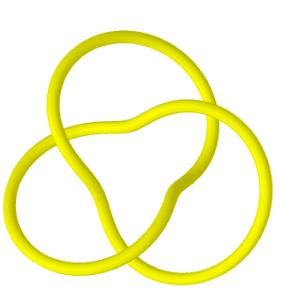
Figure 2: Trefoil knot ${\bf 3_{1}}$.

From Equation 7 and Equation 9, we have

$${}C_{\beta_{\bf 3_{1}}} = \hat{\mathfrak{R}}_{1}^{3},$$

$$\lambda_{\Lambda_{\alpha}}([r],[r]) = (-1)^{\alpha}A^{-r}q^{(\alpha^{2}-\alpha-2r\alpha+r)}.$$ (11)

Hence the colored HOMFLY-PT polynomials of trefoil knot are given by

$$H_{[r]}^{\mathcal{K}}(q,A) = \frac{1}{S^{*}_{[r]}}\sum_{\alpha}{\rm Tr}_{\mathcal{M}^{1,2}_{\Xi_{\alpha}}}(\hat{\mathfrak{R}}_{1})^{3}~{}S^{*}_{\Lambda_{\alpha}}=\frac{1}{S^{*}_{[r]}}\sum_{\alpha}\lambda_{\Lambda_{\alpha}}([r],[r])^{3}~{}S^{*}_{\Lambda_{\alpha}},$$ (12)

$$= \frac{A^{-3r}}{S^{*}_{[r]}}\sum_{\alpha=0}^{r}(-1)^{3\alpha}q^{3(\alpha^{2}-\alpha-2r\alpha+r)}~{}S^{*}_{\Lambda_{\alpha}}.$$

Here $S^{*}_{\Lambda_{\alpha}}$ is the quantum dimension of $\Lambda_{\alpha}$. The explicit colored polynomials of the trefoil knot ${\bf 3_{1}}$ for $[r]=[1],[2]$ are given below:

$$H^{{\bf 3_{1}}}_{[1]}(q,A) = \frac{A^{2}}{q^{2}}(1-A^{2}q^{2}+q^{4}),$$

$$H^{{\bf 3_{1}}}_{[2]}(q,A) = \frac{A^{4}}{q^{4}}(1-A^{2}q^{4}+q^{6}-A^{2}q^{6}+q^{8}-A^{2}q^{10}+A^{4}q^{10}+q^{12}-A^{2}q^{12}).$$

Note that as we move to the study of braids with higher number of strands, multiplicity structures may arise in the quantum $\hat{\mathfrak{R}}_{i}$-matrices. We shall illustrate the steps of the modified RT-approach for three-strand braids in the following section.

2.2 $\hat{\mathfrak{R}}$-matrices for three-strand braids

We consider a braid with $3$- strands each of which is associated with a symmetric representation $[r]$. Then, the tensor product decomposition is given as follows:

$$\bigotimes^{3}[r]=\bigoplus_{\alpha}({\rm dim}{\mathcal{M}}^{1,2,3}_{\Xi_{\alpha}})\Xi_{\alpha},$$

here the Young tableaux irreducible representations $\Xi_{\alpha}\equiv[{\xi_{1}}^{\alpha},{\xi_{2}}^{\alpha},{\xi_{3}}^{\alpha}]$ are such that ${\xi_{1}}^{\alpha}+{\xi_{2}}^{\alpha}+{\xi_{3}}^{\alpha}=3r$ and ${\xi_{1}}^{\alpha}\geq{\xi_{2}}^{\alpha}\geq{\xi_{3}}^{\alpha}\geq 0$. For example

$$\bigotimes^{3}[1] = [3,0,0]\bigoplus[1,1,1]\bigoplus 2[2,1,0].$$

First, we discuss the path and block structure of $\hat{\mathfrak{R}}$-matrix for irreducible representations $[3,0,0]$, $[1,1,1]$ and $[2,1,0]$ shown in Figure 3. Note that the multiplicity of the representations $[3,0,0]$, $[1,1,1]$, and $[2,1,0]$ is equal to one, one, and two respectively.

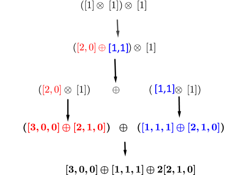
Figure 3: Path and block structures of irreducible representations $[3,0,0]$, $[1,1,1]$ and $[2,1,0]$.

Since the braid group $\mathcal{B}_{3}$ involves two braiding generators, i.e., $\hat{\mathfrak{R}}_{1}$ and $\hat{\mathfrak{R}}_{2}$-matrices. The $\hat{\mathfrak{R}}^{[2,1,0]}_{1}$-matrix is determined from the eigenvalue equation (9):

$$\hat{\mathfrak{R}}^{[2,1,0]}_{1}|[2,1,0]_{1},[2,0,0];[2,1,0]\rangle = \frac{q}{A}|[2,1,0]_{1},[2,0,0];[2,1,0]\rangle,$$ (13)

$$~{}\hat{\mathfrak{R}}^{[2,1,0]}_{1}|[2,1,0]_{2},[1,1,0];[2,1,0]\rangle = -\frac{1}{Aq}|[2,1,0]_{2},[1,1,0];[2,1,0]\rangle\rangle.$$ (14)

Hence, the explicit form of $\mathfrak{R}_{1}$ is

$$\mathfrak{R}^{[2,1,0]}_{1}=\frac{1}{A}\left(\begin{array}[]{cc}q&0\\ \\ 0&-\frac{1}{q}\end{array}\right),$$ (15)

Similarly,

$$\hat{\mathfrak{R}}^{[3,0,0]}_{1}|[3,0,0]_{1},[2,0,0];[3,0,0]\rangle = \frac{q}{A}|[3,0,0]_{1},[2,0,0];[3,0,0]\rangle,$$ (16)

$$~{}\hat{\mathfrak{R}}^{[1,1,1]}_{1}|[1,1,1]_{1},[1,1,0];[1,1,1]\rangle = -\frac{1}{Aq}|[1,1,1]_{1},[1,1,0];[1,1,1]\rangle.$$ (17)

Note that $\hat{\mathfrak{R}}_{1}$ and $\hat{\mathfrak{R}}_{2}$ cannot be simultaneously diagonal but related by a unitary matrix which can be identified with the $U_{q}(sl_{N})$ Racah matrix discussed in details in [22, 23, 17]. Therefore, from Equation 2, $\hat{\mathfrak{R}}_{2}$ is defined as

$$\hat{\mathfrak{R}}_{2}^{\Xi_{\alpha}}=\mathcal{U}^{\Xi_{\alpha}}\hat{\mathfrak{R}}_{1}^{\Xi_{\alpha}}(\mathcal{U}^{\Xi_{\alpha})^{\dagger}}.$$

Here $\mathcal{U}^{\Xi_{\alpha}\dagger}$ denotes the conjugate-transpose of $\mathcal{U}^{\Xi_{\alpha}}$. Algebraically the matrix $\mathcal{U}^{\Xi_{\alpha}}$ relates two equivalent basis states as shown below:

$$|\left(\left([r]\otimes[r]\right)_{\Lambda_{\alpha}}\otimes[r]\right)_{\Xi_{\alpha}}\rangle\xrightarrow[\text{}]{\mathcal{U}^{\Xi_{\alpha}}}|\left([r]\otimes\left([r]\otimes[r]\right)_{\Lambda_{\alpha^{\prime}}}\right)_{\Xi_{\alpha}}\rangle~{}.$$

The complete map of $\mathcal{U}^{\Xi_{\alpha}\equiv[\xi_{1}^{\alpha},\xi_{2}^{\alpha},\xi_{3}^{\alpha}]}$ matrix to $U_{q}(sl_{2})$ Racah matrix is discussed in details in [17], we have

$$\mathcal{U}^{\Xi_{\alpha}\equiv[\xi_{1}^{\alpha},\xi_{2}^{\alpha},\xi_{3}^{\alpha}]} = U_{U_{q}(sl_{2})}\begin{bmatrix}(r-{\xi_{3}}^{\alpha})/2&(r-{\xi_{3}}^{\alpha})/2\\ ~{}&~{}\\ (r-{\xi_{3}}^{\alpha})/2&({\xi_{1}}^{\alpha}-{\xi_{2}}^{\alpha})/2\end{bmatrix}.$$ (18)

The closed form expression of $U_{q}(sl_{2})$ Racah coefficients can be found in [6]. From Equation 18, the explicit form of unitary matrix $\mathcal{U}^{[2,1,0]}$ is

$$\mathcal{U}^{[2,1,0]} = U_{U_{q}(sl_{2})}\begin{bmatrix}\frac{1}{2}&\frac{1}{2}\\ ~{}&~{}\\ \frac{1}{2}&\frac{1}{2}\end{bmatrix},$$ (22)

$$= \left(\begin{array}[]{cc}\frac{1}{[2]_{q}}&\frac{\sqrt{[3]_{q}}}{[2]_{q}}\\ \\ -\frac{\sqrt{[3]_{q}}}{[2]_{q}}&\frac{1}{[2]_{q}}\end{array}\right).~{}~{}$$

Hence, the $\hat{\mathfrak{R}}_{2}$ matrices are

$${}\hat{\mathfrak{R}}^{[2,1,0]}_{2} = \mathcal{U}^{[2,1,0]}\hat{\mathfrak{R}}^{[2,1,0]}_{1}\mathcal{U}^{[2,1,0]\dagger},$$ (26)

$$= \frac{1}{A}\left(\begin{array}[]{cc}\frac{q^{2}-[3]_{q}}{q{[2]_{q}}^{2}}&-\frac{\sqrt{[3]_{q}}}{[2]_{q}}\\ \\ -\frac{\sqrt{[3]_{q}}}{[2]_{q}}&-\frac{1-q^{2}[3]_{q}}{q{[2]_{q}}^{2}}\end{array}\right).$$

Similarly,

$${}\hat{\mathfrak{R}}^{[3,0,0]}_{2} = \hat{\mathfrak{R}}^{[3,0,0]}_{1}=\frac{q}{A},$$

$$\hat{\mathfrak{R}}^{[1,1,1]}_{2} = \hat{\mathfrak{R}}^{[1,1,1]}_{1}=-\frac{1}{qA}.$$ (27)

With this description of the RT-approach for 3-stand braids, we will investigate the polynomial invariants of twisted generalized hybrid weaving knots $\hat{Q}_{3}(m_{1},-m_{2},n,\ell)$ in the next section.

3 Twisted generalized hybrid weaving knots $\hat{Q}_{3}(m_{1},-m_{2},n,\ell)$

In this section, we shall study the HOMFLY-PT polynomial of twisted generalized hybrid weaving knots. These knots, denoted hereafter as $\hat{Q}_{3}(m_{1},-m_{2},n,\ell)$, are obtained as the closure of three-strand braids

$$(\sigma_{1}^{m_{1}}\sigma_{2}^{-m_{2}})^{n}\underbrace{(\sigma_{1}\sigma_{2})^{3\ell}}_{\color[rgb]{1,0,0}twist},$$

where $m_{1},m_{2},n$ are positive integers and $\ell\in\mathbb{Z}$(see in picture 28). Notice, that without loss of generality we may assume that $m_{1}\geq m_{2}$.

(28)

It is noteworthy that the link $\hat{Q}_{3}(m_{1},-m_{2},n,\ell)$ is alternating if $\ell=0$. It is quasi-alternating non-alternating if $\ell=\pm 1$. A few examples of knots of type $\hat{Q}_{3}(m_{1},-m_{2},n,\ell)$ are given in Table 1 below.

Notation	Knot
$\hat{Q}_{3}(3,-1,1,-1)$	$5_{2}$ Knot
$\hat{Q}_{3}(5,-1,1,-1)$	$8_{20}$ Knot
$\hat{Q}_{3}(1,-1,n,0)$	weaving knot ${W}(3,n)$
$\hat{Q}_{3}(m,-m,n,0)$	hybrid weaving knot $\hat{W}_{3}(m,-m,n)$

Table 1: Examples of twisted generalized hybrid weaving knots $\hat{Q}_{3}(m_{1},-m_{2},n,\ell)$.

Now, we will apply the modified RT method and achieve a closed form expression for the HOMFLY-PT polynomials of the knots of type $\hat{Q}_{3}(m_{1},-m_{2},n,\ell)$.

3.1 HOMFLY-PT for twisted generalized hybrid weaving knots

The HOMFLY-PT polynomial corresponds to the fundamental representation ($[r]=[1]$) on each strand of the braid. The tensor product decomposition:

$$[1]^{\bigotimes 3}=[3,0,0]\bigoplus[1,1,1]\bigoplus 2[2,1,0]$$

shows that the representation $[2,1,0]$ is of multiplicity two. From Equations 7, 16 and 2.2, the HOMFLY-PT for $\hat{Q}_{3}(m_{1},-m_{2},n,\ell)$ is given by the following formula.

$$\mathcal{H}_{[1]}^{\hat{Q}_{3}(m_{1},-m_{2},n,\ell)} = \frac{1}{S^{*}_{[1]}}\sum_{\alpha}{\rm Tr}_{\Xi_{\alpha}}(\hat{\mathfrak{R}}^{\Xi_{\alpha}}_{1})^{m_{1}}(\hat{\mathfrak{R}}^{\Xi_{\alpha}}_{2})^{-m_{2}})^{n}(\hat{\mathfrak{R}}^{\Xi_{\alpha}}_{1}\hat{\mathfrak{R}}^{\Xi_{\alpha}}_{2})^{3\ell}~{},$$ (29)

$$= \frac{1}{S^{*}_{[1]}}\Bigg{(}q^{n(m_{1}-m_{2})+6\ell}S^{*}_{[3,0,0]}+(-q)^{-n(m_{1}-m_{2})-6\ell}S^{*}_{[1,1,1]}+S^{*}_{[2,1,0]}$$

$${\rm Tr}_{[2,1,0]}\Psi^{[2,1,0]}((m_{1},-m_{2},n,\ell);q)\Bigg{)}{}.$$

To obtain an explicit formula for the HOMFLYPT polynomial of $\hat{Q}_{3}(m_{1},-m_{2},n,\ell)$, we need to evaluate the trace of the matrix $\Psi^{[2,1,0]}((m_{1},-m_{2},n,\ell);q)$. Since we have

$$\Psi^{[2,1,0]}((m_{1},-m_{2},n,\ell);q)=((\hat{\mathfrak{R}}^{[2,1,0]}_{1})^{m_{1}}(\hat{\mathfrak{R}}^{[2,1,0]}_{2})^{-m_{2}}))^{n}(\hat{\mathfrak{R}}^{[2,1,0]}_{1}\hat{\mathfrak{R}}^{[2,1,0]}_{2})^{3\ell},$$

We can use Equation 15 and Equation 26 to show that

$$(\hat{\mathfrak{R}}^{[2,1,0]}_{1})^{m_{1}}(\hat{\mathfrak{R}}^{[2,1,0]}_{2})^{-m_{2}} = {A}^{-\alpha}\left(\begin{array}[]{cc}h_{1}(m_{1},m_{2})&h_{2}(m_{1},m_{2})\\ \\ \frac{h_{2}(m_{1},m_{2})}{(-1)^{m_{1}}q^{2m_{1}}}&h_{3}(m_{1},m_{2})\end{array}\right),\mbox{ and}$$

$$(\hat{\mathfrak{R}}^{[2,1,0]}_{1}\hat{\mathfrak{R}}^{[2,1,0]}_{2})^{3l} = {A}^{-\beta}\left(\begin{array}[]{cc}1&0\\ \\ 0&1\end{array}\right),$$

where

$$h_{1}(m_{1},m_{2}) = \frac{q^{\alpha}\left(1+(-1)^{m_{2}}q^{2\text{$m_{2}$}}\text{}[3]_{q}\right)}{\text{}([2]_{q})^{2}},~{}h_{2}(m_{1},m_{2})=\frac{q^{\alpha}\left(-1+(-1)^{m_{2}}q^{2\text{$m_{2}$}}\right)\sqrt{\text{}[3]_{q}}}{\text{}([2]_{q})^{2}},$$

$$h_{3}(m_{1},m_{2}) = (-1)^{\alpha}\frac{q^{-\alpha}\left(1+(-1)^{-m_{2}}q^{-2\text{$m_{2}$}}\text{}[3]_{q}\right)}{\text{}([2]_{q})^{2}},~{}\alpha=(m_{1}-m_{2}),~{}\beta=6\ell.$$

Note that as we assumed earlier, $\alpha=(m_{1}-m_{2})\geq 0$. An explicit form of $n^{th}$ power of the above matrix, denoted hereafter as $(\Psi^{[2,1,0]}((m_{1},-m_{2},n,\ell);A,q)$) is given by the following proposition.
Proposition 1.

$$\Psi^{[2,1,0]}(m_{1},-m_{2},n,l);A,q)={A}^{-\gamma}\left(\begin{array}[]{cc}\psi_{11}((m_{1},-m_{2},n);q)&\psi_{12}((m_{1},-m_{2},n-1);q)\\ \\ \ \frac{\psi_{12}((m_{1},-m_{2},n-1);q)}{(-1)^{m_{1}}q^{2m_{1}}}&\psi_{22}((m_{1},-m_{2},n);q)\end{array}\right),$$

where $\gamma=n\alpha+6\ell$, $\alpha=m_{1}-m_{2}$, and

$$\psi_{11}((m_{1},-m_{2},n);q) = \sum_{j=0}^{\lfloor\frac{n}{2}\rfloor}\sum_{k=1}^{n-j+1}(-1)^{-(m_{1}j)}\binom{k+j-2}{j-1}\binom{n-(k+j-1)}{j}$$

$$(h_{1}(m_{1},m_{2}))^{n-(2j+k-1)}(h_{3}(m_{1},m_{2}))^{k-1}(\frac{h_{2}(m_{1},m_{2})}{q^{m_{1}}})^{2j},$$

$$\psi_{22}((m_{1},-m_{2},n);q) = \sum_{j=0}^{\lfloor\frac{n}{2}\rfloor}\sum_{k=1}^{n-j+1}(-1)^{-(m_{1}j)}\binom{k+j-2}{j-1}\binom{n-(k+j-1)}{j}$$

$$(h_{3}(m_{1},m_{2}))^{n-(2j+k-1)}(h_{1}(m_{1},m_{2}))^{k-1}(\frac{h_{2}(m_{1},m_{2})}{q^{m_{1}}})^{2j},$$

$$\psi_{12}((m_{1},-m_{2},n);q) = \sum_{j=0}^{\lfloor\frac{n}{2}\rfloor}\sum_{k=1}^{n-j+1}(-1)^{-(m_{1}j)}\binom{k+j-1}{j}\binom{n-(k+j)}{j}$$

$$(h_{1}(m_{1},m_{2}))^{n-(2j+k-1)}(h_{3}(m_{1},m_{2}))^{k-1}\frac{(h_{2}(m_{1},m_{2}))^{2j+1}}{q^{2jm_{1}}}.$$

Notice that the entries in the matrix above are independent of the twist factor $\ell$ and the matrix structure is similar to the case of weaving knots $W(3,n)$, i.e., $\hat{Q}_{3}(1,-1,n,0)$ discussed in the parallel work [24]. Hence, the proof of the proposition can be done in the same way as for weaving knots. The trace of the matrix $(\Psi^{[2,1,0]}((m_{1},-m_{2},n,\ell);A,q)$ is given by

$${}\Psi^{[2,1,0]}((m_{1},-m_{2},n,\ell);A,q) = A^{-\gamma}(\psi_{11}((m_{1},-m_{2},n);q)+\psi_{22}((m_{1},-m_{2},n);q)),$$ (32)

$$= A^{-\gamma}\bigg{(}\sum_{j=0}^{\lfloor\frac{n}{2}\rfloor}\sum_{k=1}^{n-j}(-1)^{-(m_{1}j)}\binom{k+j-2}{j-1}\binom{n-(k+j-1)}{j}$$

$$\big{(}h_{1}(m_{1},m_{2}))^{(n+1-2j-k)}(h_{3}(m_{1},m_{2}))^{(k-1)}+$$

$$(h_{1}(m_{1},m_{2}))^{(k-1)}(h_{3}(m_{1},m_{2}))^{(n-2j-k+1)}\big{)}$$

$$(\frac{h_{2}(m_{1},m_{2})}{q^{m_{1}}})^{2j}\bigg{)}.$$

Substituting the parameters in Equation 32, we obtain the following expression

$${}\Psi^{[2,1,0]}((m_{1},-m_{2},n,\ell);A,q) = A^{-\gamma}\Omega((m_{1},m_{2},n);q),$$ (33)

$$\Omega((m_{1},m_{2},n);q) = (-1)^{\frac{-n\alpha}{2}}\sum_{j=0}^{\lfloor\frac{n}{2}\rfloor}\sum_{k=1}^{n-j}\binom{k+j-2}{j-1}\binom{n-(k+j-1)}{j}$$

$$G_{m_{1},-m_{2},j,k,n},$$

where

$$G_{m_{1},-m_{2},j,k,n} = \sum_{k_{1}=0}^{n+1-2j-k}\sum_{k_{2}=0}^{k-1}\sum_{k_{3}=0}^{2j}\sum_{\ell_{1}=1}^{2}\binom{n-(k+2j-1)}{k_{1}}\binom{2j}{k_{3}}\binom{k-1}{k_{2}}$$

$$\frac{{[3]_{q}}^{j+k_{1}+k_{2}}}{{[2]_{q}}^{2n}}(-1)^{\Big{(}\mu(\ell_{1})(\alpha(k-1-\frac{n}{2})+m_{2}(k_{2}-k_{1}))+k_{3}(m_{2}+1)-m_{1}j\Big{)}}$$

$$q^{\Big{(}\mu(\ell_{1})(\alpha(-2+2j+2k-n)+2m_{2}(k_{2}-k_{1}))+2m_{2}(k_{3}-j)\Big{)}},$$

here $\gamma=n\alpha+6\ell$, $\alpha=(m_{1}-m_{2})$ and $\mu(\ell_{1})$ denotes the Mobius function.

Corollary 3.1

If $m_{1}=m_{2}=m$, then the trace term reduces to

$${}(\Psi^{[2,1,0]}((m,-m,n,\ell);A,q) = A^{-6\ell}\Omega((m,m,n);q)~{}~{}~{}~{}~{}\text{where},$$

$$\Omega((m,m,n);q) = \sum_{j=0}^{\lfloor\frac{n}{2}\rfloor}\sum_{k=1}^{n-j}(-1)^{-mj}\binom{k+j-2}{j-1}\binom{n-(k+j-1)}{j}$$

$$G_{m,-m,j,k,n},$$

and

$$G_{m,-m,j,k,n} = \sum_{k_{1}=0}^{n+1-2j-k}\sum_{k_{2}=0}^{k-1}\sum_{k_{3}=0}^{2j}\sum_{\ell_{1}=1}^{2}(-1)^{\Big{(}(\mu(\ell_{1})m(k_{2}-k_{1}))+k_{3}(m+1)\Big{)}}$$

$$\binom{n-(k+2j-1)}{k_{1}}\binom{2j}{k_{3}}\binom{k-1}{k_{2}}\frac{{[3]_{q}}^{j+k_{1}+k_{2}}}{{[2]_{q}}^{2n}}$$

$$q^{2m\Big{(}\mu(\ell_{1})(k_{2}-k_{1})+(k_{3}-j)\Big{)}}.$$

The trace $\Omega((m,m,n);q)$ is a symmetric Laurent polynomial in the variable $q$. We propose the following conjecture.
Conjecture 1. Let $m$ be a natural number. Then the sum of the absolute coefficients of the Laurent polynomial $\Omega((m,m,n);q)$ is equal to the $m^{th}$ Lucas number. In other words

$${}\Omega((m,m,n);{i\mkern 1.0mu}) = {L}_{m,2n},$$ (35)

where the symbol ${L}_{m,2n}$ denotes the $m^{th}$ Lucas number generated by the $m^{th}$ Fibonacci sequence [25] and ${i\mkern 1.0mu}$ is the imaginary unit.

For clarity, we shall briefly recall the definition of the $m^{th}$ Fibonacci numbers $F_{m,n}$ and the $m^{th}$ Lucas numbers $L_{m,n}$. These are sequences ($G_{m,n}$) satisfying the Fibonacci recursive relation

$$G_{m,n+1}=mG_{m,n}+G_{m,n-1},$$

where $n\geq 1$ and the initial conditions are $F_{m,0}=0,F_{m,1}=1$, $L_{m,0}=2$, and $L_{m,1}=m$. The special cases at $m=1$, $F_{1,n}$ and $L_{1,n}$ are called classical Fibonacci and Lucas number respectively. They satisfy the following identities:

$${L}_{m,n} = {F}_{m,n-1}+{F}_{m,n+1},~{}\text{for}~{}n\geq 1,$$

$${L}^{2}_{m,n} = (m^{2}+4){F}^{2}_{m,n}+4(-1)^{n},$$

$${L}^{2}_{m,n}+{L}^{2}_{m,n+1} = (m^{2}+4){F}_{m,2n+1},$$

$${L}_{m,2n} = {L}_{m,n}^{2}+2(-1)^{n+1}.$$

The Binet Formula for $m^{th}$ Fibonacci number $F_{m,n}$ writes as

$${}F_{m,n} = \frac{\Phi_{m}^{n}-\Phi_{m}^{-n}}{\Phi_{m}+\Phi_{m}^{-1}},~{}\text{where}~{}~{}~{}\Phi_{m}=\frac{m+\sqrt{m^{2}+4}}{2}.$$ (36)

Moreover, by Theorem 2.7 of [25], we have the following formula:

$$L_{m,2n}=\frac{1}{2^{2n-1}}\sum_{j=0}^{n}\binom{2n}{2j}m^{2n-2j}(m^{2}+4)^{j}.$$

We have tabulated the first terms of the sequence $L_{m,2n}$ for few values of $m$ in Table 2.

$L_{m,2n}$	$m^{th}$ Lucas sequences for $n\geq 1$
$L_{1,2n}$	$3,7,18,47,123,322,843,2207,5778,15127,39603,103682,\ldots$
$L_{2,2n}$	$6,34,198,1154,6726,39202,228486,1331714,7761798,45239074,\ldots$
$L_{3,2n}$	$11,119,1298,14159,154451,1684802,18378371,200477279,\ldots$
$L_{4,2n}$	$18,322,5778,103682,1860498,33385282,599074578,10749957122,\ldots$
$L_{5,2n}$	$27,727,19602,528527,14250627,384238402,10360186227,\ldots$
$L_{6,2n}$	$38,1442,54758,2079362,78960998,2998438562,\ldots$
$L_{7,2n}$	$51,2599,132498,6754799,344362251,17555720002,\ldots$

Table 2: The sequence $L_{m,2n}$ for small values of $m$.

Further, $\Phi_{m}$ satisfies the following equation

$$\Phi_{m}^{2}-m\Phi_{m}-1=0.$$

Let us now test our conjecture Equation 35 in the special case $m=1,\ell=0$. The trace term reduces to

$${}\Omega((1,1,n);{i\mkern 1.0mu}) = L_{1,2n}.$$

The result coincides with what is obtained in parallel work [24]. Using Equation 33, binomial series for the trace, we get the following:
Proposition 2. The closed form expression of normalized two-variable HOMFLY-PT polynomial for twisted generalized hybrid weaving knots $\mathcal{H}_{[1]}^{\hat{Q}_{3}(m_{1},-m_{2},n,\ell)}[A,q]$ turns out to be

$${}\mathcal{H}_{[1]}^{\hat{Q}_{3}(m_{1},-m_{2},n,\ell)} = \frac{1}{S^{*}_{[1]}}\Bigg{(}\bigg{(}\frac{q}{A}\bigg{)}^{n\alpha+6\ell}S^{*}_{[3,0,0]}+(-qA)^{-n\alpha-6\ell}S^{*}_{[1,1,1]}+\bigg{(}\frac{1}{A}\bigg{)}^{n\alpha+6\ell}S^{*}_{[2,1,0]}$$

$$\cdot\Big{(}\sum_{j=0}^{\lfloor\frac{n}{2}\rfloor}\sum_{k=1}^{n-j}(-1)^{\frac{-n\alpha}{2}}\binom{k+j-2}{j-1}\binom{n-(k+j-1)}{i}G_{m_{1},-m_{2},j,k,n}\Big{)}\Bigg{)}.$$

Here

$$G_{m_{1},-m_{2},j,k,n} = \sum_{k_{1}=0}^{n+1-2j-k}\sum_{k_{2}=0}^{k-1}\sum_{k_{3}=0}^{2j}\sum_{\ell_{1}=1}^{2}\binom{n-(k+2j-1)}{k_{1}}\binom{2j}{k_{3}}\binom{k-1}{k_{2}}$$

$$\frac{{[3]_{q}}^{j+k_{1}+k_{2}}}{{[2]_{q}}^{2n}}(-1)^{\Big{(}\mu(\ell_{1})(\alpha(k-1-\frac{n}{2})+m_{2}(k_{2}-k_{1}))+k_{3}(m_{2}+1)-m_{1}j\Big{)}}$$

$$q^{\Big{(}\mu(\ell_{1})(\alpha(-2+2j+2k-n)+2m_{2}(k_{2}-k_{1}))+2m_{2}(k_{3}-j)\Big{)}},$$

and $\alpha=(m_{1}-m_{2})$, $S^{*}_{[1]}=[N]_{q}$, $S^{*}_{[3,0,0]}=\frac{[N]_{q}[N+1]_{q}[N+2]_{q}}{[2]_{q}[3]_{q}}$, $S^{*}_{[1,1,1]}=\frac{[N]_{q}[N-1]_{q}[N-2]_{q}}{[2]_{q}[3]_{q}}$, $S^{*}_{[2,1,0]}=\frac{[N]_{q}[N+1]_{q}[N-1]_{q}}{[3]_{q}}$.

Examples. If we apply the formula above to the knots $\hat{Q}_{3}(1,-1,4,-1)={\bf 10_{157}}$ and $\hat{Q}_{3}(5,-1,1,-1)={\bf 8_{20}}$, we get:

$$H^{{\bf 10_{157}}}_{[1]}(q,A) = \frac{A^{4}}{q^{6}}(-A^{2}+2q^{2}+3A^{2}q^{2}+A^{4}q^{2}-3q^{4}-5A^{2}q^{4}-3A^{4}q^{4}+4q^{6}+$$

$$6A^{2}q^{6}+3A^{4}q^{6}-3q^{8}-5A^{2}q^{8}-3A^{4}q^{8}+2q^{10}+3A^{2}q^{10}+A^{4}q^{10}$$

$$-A^{2}q^{12}).$$

$$H^{{\bf 8_{20}}}_{[1]}(q,A) = 1+2A^{2}+\frac{A^{2}}{q^{4}}-\frac{1}{q^{2}}-\frac{A^{4}}{q^{2}}-q^{2}-A^{4}q^{2}+A^{2}q^{4}.$$

Substituting $N=2$ in the formula of HOMFLY-PT in Equation 3.1, we obtain the Jones polynomial of the knot $\hat{Q}_{3}(m_{1},-m_{2},n,\ell)$

$$\mathcal{J}^{\hat{Q}_{3}(m_{1},-m_{2},n,\ell)}(q)=(q^{n(m_{1}-m_{2})+6\ell+2}+(q)^{n(m_{1}-m_{2})+6\ell-2}+\Psi^{[2,1,0]}((m_{1},-m_{2},n,\ell);q^{2},q),$$

where the explicit form of $\Psi^{[2,1,0]}((m_{1},-m_{2},n,\ell);q^{2},q)$ is as given in Equation 33.

Corollary 3.2

The Jones polynomial of the quasi-alternating knot $\hat{Q}_{3}(1,-1,n,\pm 1)$ for $n\geq 4$ is given by

$$\mathcal{J}^{\hat{Q}_{3}(1,-1,n,\pm 1)}(q)=\sum_{k=-n}^{n}(-1)^{k}\hat{J}_{(n,k,\pm 1)}q^{2k},$$

where the explicit form of $\hat{J}_{(n,k,\pm 1)}$ is

$${}\hat{J}_{(n,k,\pm 1)} = n\sum_{i=0}^{\lfloor\frac{(n-\absolutevalue{k})}{2}\rfloor}\frac{1}{n-i}\binom{n-i}{\absolutevalue{k}+i}\binom{n-\absolutevalue{k}-i-1}{i}+\delta_{k,\pm 2}+\delta_{k,\pm 4}.$$ (38)

Similarly, the Alexander polynomial $\Delta(q)$ of ${\hat{Q}_{3}(m_{1},-m_{2},n,\ell)}$ is a specialization of the HOMFLY-PT polynomial, obtained by setting $A=1$.

$${}\Delta^{\hat{Q}_{3}(m_{1},-m_{2},n,\ell)}(q)={\frac{1}{[3]_{q}}}(q^{n(m_{1}-m_{2})+6\ell}+(-q)^{-n(m_{1}-m_{2})-6\ell}-(\Psi^{[2,1,0]}((m_{1},-m_{2},n,\ell);1,q).$$

Furthermore, if $m_{1}=m_{2}=1$, we can neatly rewrite the above expression of Alexander polynomial of the knot ${\hat{Q}_{3}(1,-1,n,\ell)}$ as follows

$${}\Delta^{\hat{Q}_{3}(1,-1,n,\ell)}(q)=\Delta^{\hat{Q}_{3}(1,-1,n,0)}(q)+\sum_{-3l+2}^{3l}(-1)^{i-1}q^{2(i-1)},$$ (39)

where $\Delta^{\hat{Q}_{3}(1,-1,n,0)}(q)$ is the Alexander polynomial of weaving knots discussed in [24].

Corollary 3.3

The Alexander polynomial of the quasi-alternating knot ${\hat{Q}_{3}(1,-1,n,\pm 1)}$ for $n\geq 3$ is given by

$${}\Delta^{\hat{Q}_{3}(1,-1,n,\pm 1)}(q)=\sum^{n-1}_{i=-(n-1)}\hat{\Delta}_{(n,\absolutevalue{i})}q^{2i},$$ (40)

where

$$\hat{\Delta}_{(n,i)} = \sum^{\lfloor\frac{2n+2+i}{3}\rfloor}_{j=i+1}(-1)^{\lfloor\frac{j+i-1}{2}\rfloor}(\phi[n,\lfloor\frac{3j-i-1}{2}\rfloor]-\delta_{{i},1}+\delta_{i,2}),$$

where

$$\phi[n,k] = n\sum_{i=0}^{\lfloor\frac{(n-\absolutevalue{k})}{2}\rfloor}\frac{1}{n-i}\binom{n-i}{\absolutevalue{k}+i}\binom{n-\absolutevalue{k}-i-1}{i}.$$

For clarity, we have listed $\phi[n,k]$ for few values of $k$ in Table 3.

$k$	0	1	2	3	4
$\phi[n,n-k]$	1	$n$	$\frac{1}{2}(n-1)n$	$\frac{1}{6}n(n^{2}-3n+8)$	$\frac{1}{24}n(n-2)(n^{2}-4n+27)$

Table 3: $\phi[n,n-k]$ for $k\leq 4$.

Remark 1. The knot ${\hat{Q}_{3}(1,-1,n,\pm 1)}$ is quasi-alternating. Consequently, its link Floer homology is thin. More precisely, this homology is determined by the coefficients of the Alexander polynomial and the knot signature. Note that the signature of ${\hat{Q}_{3}(1,-1,n,\pm 1)}$ is $\pm 4$. Thus, Corollary 3.3 can be used also to find the ranks of the link Floer homology of the knot ${\hat{Q}_{3}(1,-1,n,\pm 1)}$.

3.2 The determinants of twisted hybrid weaving knots

Recall that the determinant of an oriented link $L$, ${\rm{Det}}(L)$ is a numerical invariant of links that is defined from the Seifert matrix of the link. This invariant can be obtained as the evaluation of the Alexander, or the Jones polynomial at -1, i.e., ${\rm{Det}}(L)=|\Delta^{L}(-1)|=|\mathcal{J}^{L}(-1)|$. The determinants of 3-braid links has been studied in [26]. The calculation in the previous section reveals a connection between the determinant of the knot $\hat{Q}_{3}(m,-m,n,\ell)$, where $m$ is a natural number, and the $m^{th}$ Lucas number $L_{m,2n}$. We suggest the following conjecture.
Conjecture 2. Given $m$ natural number and $\ell\in\{-1,0,1\}$, then we have:

$${}{\rm Det}(\hat{Q}_{3}(m,-m,n,0)) = |\Delta^{\hat{Q}_{3}(m,-m,n,0)}(-1)|=L_{m,2n}-2,$$

$${\rm Det}(\hat{Q}_{3}(m,-m,n,\pm 1)) = |\Delta^{\hat{Q}_{3}(m,-m,n,\pm 1)}(-1)|=L_{m,2n}+2,~{}$$ (41)

where $L_{m,2n}$ is $m^{th}$ Lucas number.
Remark 2. The classical Lucas number and golden ratio correspond to the case $m=1$. In other words, $L_{1,2n}=L_{2n}$ and $\Phi_{1}=\frac{1+\sqrt{5}}{2}$. It has been proved in [27, 28, 24] that for weaving knot $Det(W(3,n))=L_{2n}-2$.
The closed form expression obtained above for the Alexander polynomial is a good starting point to investigate the trapezoidal behavior of the Alexander polynomial of alternating closed 3-braids.

3.3 Trapezoidal Conjecture for alternating knots

In 1962, R. Fox conjectured that the coefficients of the Alexander polynomial of alternating knots are trapezoidal [29]. In other words, the absolute values of these coefficients increase, stabilize than decrease in a symmetrical way. This conjecture, known as Fox’s trapezoidal conjecture, has been confirmed for several classes of alternating knots. In particular, for some families of alternating three-braids, see [30]. We shall now prove that this conjecture holds for knots of type ${\hat{Q}_{3}(1,-1,n,\ell)}$, where $\ell=0$ or $\ell=\pm 1$.

The Alexander polynomial of knots of type ${\hat{Q}_{3}(1,-1,n,\ell)}$ in Equation 39 is given by

$${}\Delta^{\hat{Q}_{3}(1,-1,n,\ell)}(q) = \Delta^{\hat{Q}_{3}(1,-1,n,0)}(q)+\sum_{-3l+2}^{3l}(-1)^{i-1}q^{2(i-1)},$$ (42)

where $\Delta^{\hat{Q}_{3}(1,-1,n,0)}(q)$ is the Alexander polynomial of the weaving knot in [24]. Numerically, we have checked the trapezoidal conjecture for large values of $n$ and $\ell=\pm 1$ for quasi-alternating knots, see Figure 4.

$\begin{array}[]{lll}\includegraphics[width=213.39566pt]{T10.pdf}&\includegraphics[width=213.39566pt]{T20.pdf}\end{array}$

$\begin{array}[]{rr}\includegraphics[width=213.39566pt]{T50.pdf}&\includegraphics[width=213.39566pt]{T100.pdf}\end{array}$

Figure 4: The distribution of absolute values of the coefficients of Alexander polynomials of $\hat{Q}_{3}(1,-1,n,\pm 1)$.

Further, for large values of $n>>\ell$, we can prove the following.

Theorem 3.4

The asymptotic nature of the absolute values of the coefficients of the Alexander polynomial of the knot $\hat{Q}_{3}(1,-1,n,\ell)$ for $n>>\ell$ is trapezoidal, i.e.,

$${}\Delta^{\hat{Q}_{3}(1,-1,n,\ell)}(q) \equiv \Delta^{\hat{Q}_{3}(1,-1,n,0)}(q)=\sum^{n-1}_{i=-(n-1)}\mu_{(n,i)}q^{2i},~{}~{}~{}n>>\ell,$$ (43)

where,

$$\delta_{(n,i)} = \absolutevalue{\mu_{(n,i)}}-\absolutevalue{\mu_{(n,i+1)}}\geq 0.$$

Proof. Using Equation 42, we can rearrange Equation 43 such that the difference will be

$${}\delta_{(n,0)} = \absolutevalue{\mu_{(n,0)}}-\absolutevalue{\mu_{(n,1)}}=\sum^{\lfloor\frac{(2n+1)}{3}\rfloor}_{i=1}(-1)^{(\lfloor\frac{i-1}{2}\rfloor+i-1)}\left(\phi[n,\lfloor\frac{i}{2}\rfloor+i]\right).~{}$$ (44)

It is clear from Table 3 that

$$\lim_{n\to\infty}\phi[n,k]\approx\frac{n^{n-k}}{k!}$$ (45)

From Equation 44, we have

$$\delta_{(n,0)} = \sum^{\lfloor\frac{(2n+1)}{3}\rfloor}_{i=1}(-1)^{(\lfloor\frac{i-1}{2}\rfloor+i-1)}\left(\phi[n,\lfloor\frac{i}{2}\rfloor+i]\right),$$

$$= \phi[n,1]-\phi[n,3]-\phi[n,4]+\phi[n,6]+\phi[n,7]-\phi[n,9]-\phi[n,10]\ldots~{},$$

$$= n^{n-1}-\frac{n^{n-3}}{6}-\frac{n^{n-4}}{24}+\frac{n^{n-6}}{720}+\frac{n^{n-7}}{5040}-\ldots~{},\text{for large}~{}n,$$

$$= n^{n-1}(1-\frac{1}{6n^{2}}-\frac{1}{24n^{3}}+\frac{1}{720n^{5}}+\frac{1}{5040n^{6}}-\ldots).$$

From the last equality above, we can see that $\delta_{(n,0)}>0$ for large values of $n$. This completes the proof in this case. A similar argument can be used to prove that $\delta_{(n,i)}\geq 0$ for any value of $i$.

4 Colored HOMFLY-PT for twisted weaving knots $\hat{Q}_{3}(1,-1,n,\ell)$

In the previous section, we have derived an explicit formula for the trace of $2\otimes 2$ matrices (32) and HOMFLY-PT polynomial (3.1) corresponding to the representation $[r]=[1]$. In the following sub-section we shall discuss the generalization of these results to higher colors $[r]>1$.

4.1 Trace terms for representations $[r]>1$

Given a representation $[r]>[1]$, the irreducible representation $\Xi_{\alpha}\equiv[{\xi_{1}}^{\alpha},{\xi_{2}}^{\alpha},{\xi_{3}}^{\alpha}]\in[r]^{\otimes 3}$ has multiplicity $(M)$ arising from path structure of $\Lambda_{\alpha,\mu}\in[r]^{\otimes 2}$. Here, $\mu$ takes the values $0,1,\ldots M-1$ and keeps track of multiplicity. Corresponding block diagonal matrix $\hat{\mathfrak{R}}^{\Xi_{\alpha}}_{1}$ entries are

$$\pm\{q^{\chi_{r,0}},-q^{\chi_{r,1}},\ldots(-1)^{M-1}q^{\chi_{r,M-1}}\},$$

and $\hat{\mathfrak{R}}^{\Xi_{\alpha}}_{2}=\mathcal{U}^{\Xi_{\alpha}}\hat{\mathfrak{R}}^{\Xi_{\alpha}}_{1}\mathcal{U}^{\Xi_{\alpha}}$. After analyzing numerous examples of twisted weaving knots of braid index 3, we propose the following:
Proposition 3.

$${}(\hat{\mathfrak{R}}_{1}^{\Xi_{\alpha}}\hat{\mathfrak{R}}_{2}^{\Xi_{\alpha}})^{3\ell} = q^{\Lambda_{M}}\mathcal{I}_{M\times M},$$

$${\rm Tr}(\hat{\mathfrak{R}}_{1}^{\Xi_{\alpha}}(\hat{\mathfrak{R}}_{2}^{\Xi_{\alpha}})^{-1})^{n}(\hat{\mathfrak{R}}_{1}^{\Xi_{\alpha}}\hat{\mathfrak{R}}_{2}^{\Xi_{\alpha}})^{3\ell} = q^{\Lambda_{M}}{\rm Tr}(\hat{\mathfrak{R}}_{1}^{\Xi_{\alpha}}(\hat{\mathfrak{R}}_{2}^{\Xi_{\alpha}})^{-1})^{n},$$ (46)

here, ${\Lambda_{M}}$ is a twist factor which depends on parameters $\{\chi_{r,0},\chi_{r,1},\dots\chi_{r,M-1},\ell\}$ and $\mathcal{I}_{M\times M}$ is identity matrix of size $M$.
By checking several examples, we compute the twist factors for $M=2$ and $3$

$$\Lambda_{2}={3(\chi_{r,0}+\chi_{r,1})\ell},{\rm{and}}~{}~{}\Lambda_{3}={2(\chi_{r,0}+\chi_{r,1}+\chi_{r,2})\ell}.$$

At the moment it is difficult to guess a closed form of $\Lambda_{M}$ for $M\geq 4$. Let

$$\Theta_{n,t,m,\ell}[q]={\rm Tr}(\hat{\mathfrak{R}}_{1}^{\Xi_{\alpha}}(\hat{\mathfrak{R}}_{2}^{\Xi_{\alpha}})^{-1})^{n}(\hat{\mathfrak{R}}_{1}^{\Xi_{\alpha}}\hat{\mathfrak{R}}_{2}^{\Xi_{\alpha}})^{\ell}.$$

The following conjecture generalizes Proposition 1 in [5].
Conjecture 3. Given a representation $\Xi_{\alpha}\equiv[{\xi_{1}}^{\alpha},{\xi_{2}}^{\alpha},{\xi_{3}}^{\alpha}]$ having multiplicity 2 with $\hat{\mathfrak{R}}^{\Xi_{\alpha}}_{1}=\pm\left(\begin{array}[]{cc}q^{t+m}&0\\ \\ 0&-q^{-t+m}\end{array}\right)$, $\hat{\mathfrak{R}}^{\Xi_{\alpha}}_{2}=\mathcal{U}^{\Xi_{\alpha}}\hat{\mathfrak{R}}^{\Xi_{\alpha}}_{1}\mathcal{U}^{\Xi_{\alpha}}$, and  $\mathcal{U}^{\Xi_{\alpha}}=\left(\begin{array}[]{cc}\frac{1}{[2]_{q^{t}}}&\frac{\sqrt{[3]_{q^{t}}}}{[2]_{q^{t}}}\\ \frac{\sqrt{[3]_{q^{t}}}}{[2]_{q^{t}}}&-\frac{1}{[2]_{q^{t}}}\end{array}\right).\ \$ Then

$${}\Theta_{n,t,m,\ell}[q] = q^{\Lambda_{2}}{\rm Tr}(\hat{\mathfrak{R}}_{1}^{\Xi_{\alpha}}(\hat{\mathfrak{R}}_{2}^{\Xi_{\alpha}})^{-1})^{n},$$ (47)

$$= \sum_{g=-n}^{n}(-1)^{g}\Omega_{n,n-\absolutevalue{g}}q^{2gt+6m\ell}.$$

Here $t$ and $m$ are integers which dependent on $\Xi_{\alpha}$ and the coefficients $\Omega_{n,j}$ are given by the following formula:

$$\Omega_{n,j} = \sum_{i=0}^{\lfloor\frac{j}{2}\rfloor}\frac{n}{n-i}\binom{n-i}{n-j+i}\binom{j-i-1}{i}~{},$$

where the parameters $n$ and $j$ are positive integers, $|x|$ denotes the absolute value of $x$ and $\lfloor x\rfloor$ indicates the greatest integer less than or equal to $x$.
In the following subsections, we will use Equations 4.1 and 47 to compute the $[r]$-colored HOMFLY-PT polynomials of $\hat{Q}_{3}(1,-1,n,\ell)$ for $[r]=[2],[3],\text{and}~{}[4]$.

4.2 HOMFLY-PT polynomial of the knots $\hat{Q}_{3}(1,-1,n,\ell)$

The HOMFLY-PT polynomial of the knot $\hat{Q}_{3}(1,-1,n,\ell)$ is given by the following formula:

$${}\mathcal{H}_{[1]}^{\hat{Q}_{3}(1,-1,n,\ell)}(A,q)=\frac{1}{S^{*}_{[1]}}(q^{6\ell}S^{*}_{[3]}+(-q)^{-6\ell})S^{*}_{[111]}+S^{*}_{[21]}\Theta_{n,1,0,\ell}[q]).$$ (48)

Substituting $A=q^{2}$, we get the Jones polynomial:

$$\mathcal{J}^{\hat{Q}_{3}(1,-1,n,\ell)}(q)=q^{-2+6\ell}+q^{2+6\ell}+\Theta_{n,1,0,\ell}[q]~{}.$$

We will use the data on $U^{\Xi_{\alpha}}$ matrices in Section 2.2 for three-strand braids where $\Xi_{\alpha}\in[r]^{3}$ to compute the $[r]$-colored HOMFLY-PT polynomials of the twisted weaving knots $\hat{Q}_{3}(1,-1,n,\ell)$.

4.3 $[2]$-colored HOMFLY-PT polynomial of the knots $\hat{Q}_{3}(1,-1,n,\ell)$

In the case $[r]=[2]$, the tensor product decomposition rules are as follows:

$$\bigotimes^{3}[2]=[6,0,0]\bigoplus[3,3,0]\bigoplus[4,1,1]\bigoplus[2,2,2]\bigoplus 2[5,1,0]\bigoplus 2[3,2,1]\bigoplus 3[4,2,0].$$

It can be easily seen that there are one $3\times 3$-matrix, one $2\times 2$-matrix and two $1\times 1$-matrices. The twisted trace (47) and twist factor (4.1) are shown in the Table 4.

$\Xi_{\alpha}\in[2]^{3}$	Matrix size (M)	Trace $\Theta_{n,t,m,\ell}[q]$	Twist factor $\Lambda_{M}$
[3,2,1]	2	$\Theta_{n,1,1,\ell}[q]$	$6\ell$
[5,1,0]	2	$\Theta_{n,2,4,\ell}[q]$	$24\ell$
[4,2,0]	3	To be determined	$16\ell$

Table 4: Twisted trace and twisted factor table for $\Xi_{\alpha}\in[2]^{\otimes 3}$.

The eigenvalues matrices in this case are

$$\hat{\mathfrak{R}}^{[5,1,0]}_{1}=q^{4}\left(\begin{array}[]{cc}q^{2}&0\\ 0&-q^{-2}\\ \end{array}\right)\\ ,~{}~{}\hat{\mathfrak{R}}^{[4,2,0]}_{1}=\left(\begin{array}[]{ccc}1&0&0\\ 0&-q^{2}&0\\ 0&0&q^{6}\\ \end{array}\right),$$

and

$$\hat{\mathfrak{R}}^{[3,2,1]}_{1}=q\left(\begin{array}[]{cc}q^{-1}&0\\ 0&-q\\ \end{array}\right),\ \$$ (49)

and the corresponding $U^{\Xi_{\alpha}}$ extracted from Equation 18. From Equation 7, the $[2]$-HOMFLY-PT for $\hat{Q}_{3}(1,-1,n,\ell)$ can be expressed as follows:

$$\mathcal{H}_{[2]}^{\hat{Q}_{3}(1,-1,n,\ell)} = \frac{A^{-12\ell}q^{-24\ell}}{S^{*}_{[2]}}(S^{*}_{[2,2,2]}+q^{36\ell}S^{*}_{[6]}+(-q)^{12\ell}S^{*}_{[3,3]}+(-q)^{12\ell}S^{*}_{[4,1,1]}+$$ (50)

$$S^{*}_{[5,1]}{\rm Tr}_{[5,1,0]}(\hat{\mathfrak{R}}^{[5,1,0]}_{1}(\hat{\mathfrak{R}}^{[5,1,0]}_{2})^{-1})^{n}(\hat{\mathfrak{R}}^{[5,1,0]}_{1}\hat{\mathfrak{R}}^{[5,1,0]}_{2})^{3\ell}$$

$$+S^{*}_{[3,2,1]}{\rm Tr}_{[3,2,1]}(\hat{\mathfrak{R}}^{[3,2,1]}_{1}\hat{\mathfrak{R}}^{[3,2,1]}_{2})^{-1})^{n}(\hat{\mathfrak{R}}^{[3,2,1]}_{1}\hat{\mathfrak{R}}^{[3,2,1]}_{2})^{3\ell}$$

$$+S^{*}_{[4,2,0]}{\rm Tr}_{[4,2,0]}(\hat{\mathfrak{R}}^{[4,2,0]}(\hat{\mathfrak{R}}^{[4,2,0]}_{2})^{-1})^{n}(\hat{\mathfrak{R}}^{[4,2,0]}_{1}\hat{\mathfrak{R}}^{[4,2,0]}_{2})^{3\ell}{}.$$

Using Table 4, we can rewrite Equation (50) into a more concise formula

$$\mathcal{H}_{[2]}^{\hat{Q}_{3}(1,-1,n,\ell)} = \frac{A^{-12\ell}q^{-24\ell}}{S^{*}_{[2]}}(S^{*}_{[2,2,2]}+q^{36\ell}S^{*}_{[6,0,0]}+(-q)^{12\ell}S^{*}_{[4,1,1]}+(-q)^{12\ell}S^{*}_{[3,3,0]}$$

$$+S^{*}_{[5,1]}\Theta_{n,2,4,\ell}[q]+S^{*}_{[3,2,1]}\Theta_{n,1,1,\ell}[q]+q^{16\ell}S^{*}_{[4,2,0]}{\rm Tr}(X^{[4,2,0]})^{n},$$

(51)

where,

$$X^{[4,2,0]}=\left(\begin{array}[]{ccc}\frac{1}{q^{6}+q^{8}+q^{10}}&-\frac{1}{q^{5}\sqrt{1+q^{2}+q^{4}}}&\frac{\sqrt{1+q^{2}+q^{4}+q^{6}+q^{8}}}{q^{2}+q^{4}+q^{6}}\\ \frac{1}{q^{3}\sqrt{1+q^{2}+q^{4}}}&\frac{-1+q^{2}-q^{4}}{q^{2}+q^{6}}&-\frac{q^{3}\sqrt{\frac{1+q^{2}+q^{4}+q^{6}+q^{8}}{1+q^{2}+q^{4}}}}{1+q^{4}}\\ \frac{q^{4}\sqrt{1+q^{2}+q^{4}+q^{6}+q^{8}}}{1+q^{2}+q^{4}}&\frac{q^{7}\sqrt{\frac{1+q^{2}+q^{4}+q^{6}+q^{8}}{1+q^{2}+q^{4}}}}{1+q^{4}}&\frac{q^{14}}{1+q^{2}+2q^{4}+q^{6}+q^{8}}\\ \end{array}\right).$$ (52)

It is worth mentioning here that the $[2]$-colored polynomial in Equation 50 for arbitrary $n$ and $\ell$ are easily computable. We have listed $[2]$-colored polynomials in Appendix 8 for some twisted weaving knots.

4.4 $[3]$-colored HOMFLY-PT polynomial of the knots $\hat{Q}_{3}(1,-1,n,\ell)$

The tensor product decomposition rules in this case writes as follows:

$$\bigotimes^{3}[3] = [9,0,0]\bigoplus[7,1,1]\bigoplus[5,2,2]\bigoplus[4,4,1]\bigoplus[3,3,3]\bigoplus 3[8,1,0]$$

$$\bigoplus 2[4,3,2]\bigoplus 2[6,2,1]\bigoplus 2[5,4,0]\bigoplus 3[7,2,0]\bigoplus 3[5,3,1]$$

$$\bigoplus 4[6,3,0].$$

Thus, we have two $3\times 3$-matrices, one $2\times 2$-matrix, one $1\times 1$-matrix and one $4\times 4$-matrix as tabulated below.

$\Xi_{\alpha}\in[3]^{3}$	Matrix size $(M)$	Trace $\Theta_{n,t,m,\ell}[q]$	Twist factor $\Lambda_{M,}$
[4,3,2]	2	$\Theta_{n,1,4,\ell}[q]$	${24\ell}$
[6,2,1]	2	$\Theta_{n,2,7,\ell}[q]$	${42\ell}$
[5,4,0]	2	$\Theta_{n,2,7,\ell}[q]$	${42\ell}$
[8,1,0]	2	$\Theta_{n,3,12,\ell}[q]$	${72\ell}$
[7,2,0]	3	To be determined	${58\ell}$
[5,3,1]	3	To be determined	${34\ell}$
[6,3,0]	4	To be determined	${48\ell}$

Table 5: Twisted trace and twisted factors table for $\Xi_{\alpha}\in[3]^{\otimes 3}$.

The braiding matrices in this case are

$${}~{}{\hat{\mathfrak{R}}^{[6,3,0]}=\left(\begin{array}[]{cccc}-q^{3}&0&0&0\\ 0&q^{5}&0&0\\ 0&0&-q^{9}&0\\ 0&0&0&q^{15}\\ \end{array}\right)}\\ ,~{}~{}{\hat{\mathfrak{R}}^{[5,3,1]}=\left(\begin{array}[]{ccc}-q^{3}&0&0\\ 0&q^{5}&0\\ 0&0&-q^{9}\\ \end{array}\right)}\\ ,$$

$${}{\hat{\mathfrak{R}}^{[7,2,0]}=\left(\begin{array}[]{ccc}q^{5}&0&0\\ 0&-q^{9}&0\\ 0&0&q^{15}\\ \end{array}\right)}~{},\hat{\mathfrak{R}}^{[5,4,0]}=\hat{\mathfrak{R}}^{[6,2,1]}=q^{7}\left(\begin{array}[]{cc}q^{-2}&0\\ 0&-q^{2}\\ \end{array}\right)\\ ,~{}~{}~{}$$

$$\hat{\mathfrak{R}}^{[4,3,2]}=q^{4}\left(\begin{array}[]{cc}-q^{-1}&0\\ 0&q\\ \end{array}\right)\\ ,~{}{\hat{\mathfrak{R}}^{[8,1,0]}=q^{12}\left(\begin{array}[]{cc}-q^{-3}&0\\ 0&q^{3}\\ \end{array}\right)},$$

and $U^{\Xi_{\alpha}}$ matrices computed from Equation 18. Using the Equation 7, the $[3]$-colored HOMFLY-PT polynomial of $\hat{Q}_{3}(1,-1,n,\ell)$ is as given below:

$$\mathcal{H}_{[3]}^{\hat{Q}_{3}(1,-1,n,\ell)} = \frac{A^{-36\ell}q^{-72\ell}}{S^{*}_{[3]}}\sum_{\alpha}{\rm Tr}_{\Xi_{\alpha}}(\hat{\mathfrak{R}}^{\Xi_{\alpha}}_{1})(\hat{\mathfrak{R}}^{\Xi_{\alpha}}_{2})^{-1})^{n}(\hat{\mathfrak{R}}^{\Xi_{\alpha}}_{1}\hat{\mathfrak{R}}^{\Xi_{\alpha}}_{2})^{3\ell}~{},$$ (53)

$$= \frac{1}{S^{*}_{[3]}}(q^{90\ell}S^{*}_{[9]}+(-q)^{54\ell}S^{*}_{[7,1,1]}+q^{30\ell}S^{*}_{[5,2,2]}+q^{30\ell}S^{*}_{[4,4,1]}+(-q)^{18\ell}$$

$$S^{*}_{[3,3,3]}+S^{*}_{[5,4,0]}{\rm Tr}_{[5,4,0]}(\hat{\mathfrak{R}}^{[5,4,0]}_{1}(\hat{\mathfrak{R}}^{[5,4,0]}_{2})^{-1})^{n}(\hat{\mathfrak{R}}^{[5,4,0]}_{1}\hat{\mathfrak{R}}^{[5,4,0]}_{2})^{3\ell}+$$

$$S^{*}_{[4,3,2]}{\rm Tr}_{[4,3,2]}(\hat{\mathfrak{R}}^{[4,3,2]}_{1}(\hat{\mathfrak{R}}^{[4,3,2]}_{2})^{-1})^{n}(\hat{\mathfrak{R}}^{[4,3,2]}_{1}\hat{\mathfrak{R}}^{[4,3,2]}_{2})^{3\ell}+S^{*}_{[6,2,1]}$$

$${\rm Tr}_{[6,2,1]}(\hat{\mathfrak{R}}^{[6,2,1]}_{1}(\hat{\mathfrak{R}}^{[6,3,1]}_{2})^{-1})^{n}(\hat{\mathfrak{R}}^{[6,2,1]}_{1}\hat{\mathfrak{R}}^{[6,2,1]}_{2})^{3\ell}+S^{*}_{[8,1,0]}$$

$${\rm Tr}_{[8,1,0]}(\hat{\mathfrak{R}}^{[8,1,0]}_{1}(\hat{\mathfrak{R}}^{[8,1,0]}_{2})^{-1})^{n}(\hat{\mathfrak{R}}^{[8,1,0]}_{1}\hat{\mathfrak{R}}^{[8,1,0]}_{2})^{3\ell}+S^{*}_{[7,2,0]}$$

$${\rm Tr}_{[7,2,0]}(\hat{\mathfrak{R}}^{[7,2,0]}_{1}\hat{\mathfrak{R}}^{[7,2,0]}_{2})^{-1})^{n}(\hat{\mathfrak{R}}^{[7,2,0]}_{1}\hat{\mathfrak{R}}^{[7,2,0]}_{2})^{3\ell}+S^{*}_{[5,3,1]}$$

$${\rm Tr}_{[5,3,1]}(\hat{\mathfrak{R}}^{[5,3,1]}_{1}\hat{\mathfrak{R}}^{[5,3,1]}_{2})^{-1})^{n}(\hat{\mathfrak{R}}^{[5,3,1]}_{1}\hat{\mathfrak{R}}^{[5,3,1]}_{2})^{3\ell}+S^{*}_{[6,3,0]}$$

$${\rm Tr}_{[6,3,0]}(\hat{\mathfrak{R}}^{[6,3,0]}_{1}(\hat{\mathfrak{R}}^{[6,3,0]}_{2})^{-1})^{n}(\hat{\mathfrak{R}}^{[6,3,0]}_{1}\hat{\mathfrak{R}}^{[6,3,0]}_{2})^{3\ell}{}.$$

Using Table 6, we can rewrite Equation 53 into the following formula

$$\mathcal{H}_{[3]}^{\hat{Q}_{3}(1,-1,n,\ell)} = \frac{A^{-18\ell}q^{-72\ell}}{S^{*}_{[3]}}(q^{90\ell}S^{*}_{[9]}+(-q)^{54\ell}S^{*}_{[7,1,1]}+q^{30\ell}S^{*}_{[5,2,2]}+q^{30\ell}S^{*}_{[4,4,1]}$$ (54)

$$+(-q)^{18\ell}S^{*}_{[3,3,3]}+S^{*}_{[5,4,0]}\Theta_{n,2,7,\ell}[q]+S^{*}_{[6,2,1]}\Theta_{n,2,7,\ell}[q]+S^{*}_{[4,3,2]}$$

$$\Theta_{n,1,4,\ell}[q]+S^{*}_{[8,1,0]}\Theta_{n,3,12,\ell}[q]+q^{58\ell}S^{*}_{[7,2,0]}{\rm Tr}(X_{1}^{[7,2,0]})^{n}+q^{34\ell}$$

$$S^{*}_{[5,3,1]}{\rm Tr}(X_{1}^{[5,3,1]})^{n}+q^{48\ell}S^{*}_{[6,3,0]}{\rm Tr}(X_{3}^{[6,3,0]})^{n}.{}$$

Where the explicit forms of $X_{1}^{[7,2,0]}$, $X_{2}^{[5,3,1]}$, and $X_{3}^{[6,3,0]}$ are given in Appendix 7 and algebraic polynomial forms of 54 are presented in Appendix 8.

4.5 $[4]$-colored HOMFLY-PT polynomial of the knots $\hat{Q}_{3}(1,-1,n,\ell)$

In this case, the tensor product decomposition rules are as follows:

$$\bigotimes^{3}[4] = [12,0,0]\bigoplus[10,1,1]\bigoplus[8,2,2]\bigoplus[6,6,0]\bigoplus[6,3,3]\bigoplus[5,2,2]\bigoplus[4,4,4]$$

$$\bigoplus 2[11,1,0]\bigoplus 2[9,2,1]\bigoplus 2[7,3,2]\bigoplus 2[6,5,1]\bigoplus 2[5,4,3]\bigoplus 3[10,2,0]$$

$$\bigoplus 3[7,5,0]\bigoplus 3[7,4,1]\bigoplus 3[6,4,2]\bigoplus 4[7,4,1]\bigoplus 4[9,3,0]\bigoplus 5[8,4,0].$$

Thus, we have one $5\times 5$-matrix, two $4\times 4$-matrices, four $3\times 3$-matrices, five $2\times 2$-matrices and six $1\times 1$-matrices.

$\Xi_{\alpha}\in[4]^{3}$	Matrix size $(M)$	Trace $\Theta_{n,t,m,\ell}[q]$	Twist factor $\Lambda_{M}$
[9,2,1]	2	$\Theta_{n,3,17,\ell}[q]$	${102\ell}$
[7,3,2]	2	$\Theta_{n,2,12,\ell}[q]$	${72\ell}$
[11,1,0]	2	$\Theta_{n,4,24,\ell}[q]$	${144\ell}$
[6,5,1]	2	$\Theta_{n,2,12,\ell}[q]$	${72\ell}$
[5,4,1]	2	$\Theta_{n,1,9,\ell}[q]$	${54\ell}$
[10,2,0]	3	To be determined	${124\ell}$
[8,3,1]	3	To be determined	${88\ell}$
[7,5,0]	3	To be determined	${88\ell}$
[6,4,2]	3	To be determined	${64\ell}$
[9,3,0]	4	To be determined	${108\ell}$
[7,4,1]	4	To be determined	${78\ell}$
[8,4,0]	5	To be determined	${96\ell}$

Table 6: Twisted trace and twisted factors table for $\Xi_{\alpha}\in[4]^{\otimes 3}$.

The braiding matrices in this case are

$${}\hat{\mathfrak{R}}^{[11,1,0]}=\left(\begin{array}[]{cc}-q^{20}&0\\ 0&q^{28}\\ \end{array}\right),\hat{\mathfrak{R}}^{[9,2,1]}=\left(\begin{array}[]{cc}q^{14}&0\\ 0&-q^{20}\\ \end{array}\right),\hat{\mathfrak{R}}^{[5,4,3]}=\left(\begin{array}[]{cc}q^{8}&0\\ 0&-q^{10}\\ \end{array}\right),$$

$${}\hat{\mathfrak{R}}^{[7,3,2]}=\hat{\mathfrak{R}}^{[6,5,1]}=\left(\begin{array}[]{cc}-q^{10}&0\\ 0&q^{14}\\ \end{array}\right),\hat{\mathfrak{R}}^{[10,2,0]}=\left(\begin{array}[]{ccc}q^{14}&0&0\\ 0&-q^{20}&0\\ 0&0&q^{28}\\ \end{array}\right),$$

$${}\hat{\mathfrak{R}}^{[6,4,2]}=\left(\begin{array}[]{ccc}q^{8}&0&0\\ 0&-q^{10}&0\\ 0&0&q^{14}\\ \end{array}\right),~{}\hat{\mathfrak{R}}^{[7,5,0]}=\hat{\mathfrak{R}}^{[8,3,1]}=\left(\begin{array}[]{ccc}-q^{10}&0&0\\ 0&q^{14}&0\\ 0&0&-q^{20}\\ \end{array}\right),$$

$$\hat{\mathfrak{R}}^{[9,3,0]}=\left(\begin{array}[]{cccc}-q^{10}&0&0&0\\ 0&q^{14}&0&0\\ 0&0&-q^{20}&0\\ 0&0&0&q^{28}\\ \end{array}\right),$$

$$\hat{\mathfrak{R}}^{[7,4,1]}=\left(\begin{array}[]{cccc}q^{8}&0&0&0\\ 0&-q^{10}&0&0\\ 0&0&q^{14}&0\\ 0&0&0&-q^{20}\\ \end{array}\right),~{}\hat{\mathfrak{R}}^{[8,4,0]}=\left(\begin{array}[]{ccccc}q^{8}&0&0&0&0\\ 0&-q^{10}&0&0&0\\ 0&0&q^{14}&0&0\\ 0&0&0&-q^{20}&0\\ 0&0&0&0&q^{28}\\ \end{array}\right),~{}$$ (55)

and $U^{\Xi_{\alpha}}$ matrices computed from Equation 18. From Equation 7, the $[4]$-colored HOMFLY-PT polynomial of $\hat{Q}_{3}(1,-1,n,\ell)$ can be expressed as follows:

$$\mathcal{H}_{[4]}^{\hat{Q}_{3}(1,-1,n,\ell)} = \frac{A^{-24\ell}q^{-144\ell}}{S^{*}_{[4}}\sum_{\alpha}{\rm Tr}_{\Xi_{\alpha}}(\hat{\mathfrak{R}}^{\Xi_{\alpha}}_{1})(\hat{\mathfrak{R}}^{\Xi_{\alpha}}_{2})^{-1})^{n}(\hat{\mathfrak{R}}^{\Xi_{\alpha}}_{1}\hat{\mathfrak{R}}^{\Xi_{\alpha}}_{2})^{3\ell}~{},$$ (56)

$$= \frac{1}{S^{*}_{[4]}}(q^{168\ell}S^{*}_{[12]}+(-q)^{120\ell}S^{*}_{[10,1,1]}+q^{84\ell}S^{*}_{[8,2,2]}+q^{84\ell}S^{*}_{[6,6]}+(-q)^{60\ell}$$

$$S^{*}_{[6,3,3]}+(-q)^{60\ell}S^{*}_{[5,5,2]}+S^{*}_{[11,2,0]}{\rm Tr}_{[11,2,0]}(\hat{\mathfrak{R}}^{[11,2,0]}_{1}(\hat{\mathfrak{R}}^{[11,2,0]}_{2})^{-1})^{n}$$

$$(\hat{\mathfrak{R}}^{[11,2,0]}_{1}\hat{\mathfrak{R}}^{[11,2,0]}_{2})^{3\ell}+S^{*}_{[9,2,1]}{\rm Tr}_{[9,2,1]}(\hat{\mathfrak{R}}^{[9,2,1]}_{1}(\hat{\mathfrak{R}}^{[9,2,1]}_{2})^{-1})^{n}(\hat{\mathfrak{R}}^{[9,2,1]}_{1}\hat{\mathfrak{R}}^{[9,2,1]}_{2})^{3\ell}$$

$$+S^{*}_{[7,3,2]}{\rm Tr}_{[7,3,2]}(\hat{\mathfrak{R}}^{[7,3,2]}_{1}(\hat{\mathfrak{R}}^{[7,3,2]}_{2})^{-1})^{n}(\hat{\mathfrak{R}}^{[7,3,2]_{1}}\hat{\mathfrak{R}}^{[7,3,2]}_{2})^{3\ell}+S^{*}_{[6,5,1]}$$

$${\rm Tr}_{[6,5,1]}(\hat{\mathfrak{R}}^{[6,5,1]}_{1}(\hat{\mathfrak{R}}^{[6,5,1]}_{2})^{-1})^{n}(\hat{\mathfrak{R}}^{[6,5,1]}_{1}\hat{\mathfrak{R}}^{[6,5,1]}_{2})^{3\ell}+S^{*}_{[5,4,3]}{\rm Tr}_{[5,4,3]}$$

$$(\hat{\mathfrak{R}}^{[5,4,3]}_{1}(\hat{\mathfrak{R}}^{[5,4,3]}_{2})^{-1})^{n}(\hat{\mathfrak{R}}^{[5,4,3]}_{1}\hat{\mathfrak{R}}^{[5,4,3]}_{2})^{3\ell}+S^{*}_{[10,2,0]}{\rm Tr}_{[10,2,0]}$$

$$(\hat{\mathfrak{R}}^{[10,2,0]}_{1}(\hat{\mathfrak{R}}^{[10,2,0]}_{2})^{-1})^{n}(\hat{\mathfrak{R}}^{[10,2,0]}_{1}\hat{\mathfrak{R}}^{[10,2,0]}_{2})^{3\ell}+S^{*}_{[7,5,0]}{\rm Tr}_{[7,5,0]}$$

$$(\hat{\mathfrak{R}}^{[7,5,0]}_{1}\hat{\mathfrak{R}}^{[7,5,0]}_{2})^{-1})^{n}(\hat{\mathfrak{R}}^{[7,5,0]}_{1}\hat{\mathfrak{R}}^{[7,5,0]}_{2})^{3\ell}+S^{*}_{[6,4,2]}{\rm Tr}_{[6,4,2]}$$

$$(\hat{\mathfrak{R}}^{[6,4,2]}_{1}(\hat{\mathfrak{R}}^{[6,4,2]}_{2})^{-1})^{n}(\hat{\mathfrak{R}}^{[6,4,2]}_{1}\hat{\mathfrak{R}}^{[6,4,2]}_{2})^{3\ell}+S^{*}_{[9,3,0]}{\rm Tr}_{[9,3,0]}$$

$$(\hat{\mathfrak{R}}^{[9,3,0]}_{1}(\hat{\mathfrak{R}}^{[9,3,0]}_{2})^{-1})^{n}(\hat{\mathfrak{R}}^{[9,3,0]}_{1}\hat{\mathfrak{R}}^{[9,3,0]}_{2})^{3\ell}+S^{*}_{[7,4,1]}{\rm Tr}_{[7,4,1]}$$

$$(\hat{\mathfrak{R}}^{[7,4,1]}_{1}(\hat{\mathfrak{R}}^{[7,4,1]}_{2})^{-1})^{n}(\hat{\mathfrak{R}}^{[7,4,1]}_{1}\hat{\mathfrak{R}}^{[7,4,1]}_{2})^{3\ell}+S^{*}_{[8,4,0]}{\rm Tr}_{[8,4,0]}$$

$$(\hat{\mathfrak{R}}^{[8,4,0]}_{1}(\hat{\mathfrak{R}}^{[8,4,0]}_{2})^{-1})^{n}(\hat{\mathfrak{R}}^{[8,4,0]}_{1}\hat{\mathfrak{R}}^{[8,4,0]}_{2})^{3\ell}.{}$$

Using Table 6, we can rewrite Equation 56 into the following

$$\mathcal{H}_{[4]}^{\hat{Q}_{3}(1,-1,n,\ell)} = \frac{A^{-24\ell}q^{-144\ell}}{S^{*}_{[4]}}(q^{168\ell}S^{*}_{[12]}+(-q)^{120\ell}S^{*}_{[10,1,1]}+q^{84\ell}S^{*}_{[8,2,2]}+q^{84\ell}S^{*}_{[6,6]}+$$ (57)

$$(-q)^{60\ell}S^{*}_{[6,3,3]}+(-q)^{60\ell}S^{*}_{[5,5,2]}+S^{*}_{[11,1,0]}\Theta_{n,4,24,\ell}[q]+S^{*}_{[9,2,1]}\Theta_{n,3,17,\ell}[q]+$$

$$S^{*}_{[7,3,2]})\Theta_{n,2,12,\ell}[q]+S^{*}_{[6,5,1]}\Theta_{n,2,12,\ell}[q]+S^{*}_{[5,4,3]}\Theta_{n,1,9,\ell}[q]+q^{124\ell}S^{*}_{[10,2,0]}$$

$${\rm Tr}(X_{1}^{[10,2,0]})^{n}+q^{88\ell}S^{*}_{[7,5,0]}{\rm Tr}(X_{2}^{[7,5,0]})^{n}+q^{64\ell}S^{*}_{[6,4,2]}{\rm Tr}(X_{3}^{[6,4,2]})^{n}+q^{108\ell}$$

$$S^{*}_{[9,3,0]}{\rm Tr}(X_{4}^{[9,3,0]})^{n}+q^{78\ell}S^{*}_{[7,4,1]}{\rm Tr}(X_{5}^{[7,4,1]})^{n}+q^{96\ell}S^{*}_{[8,4,0]}{\rm Tr}(X_{6}^{[8,4,0]})^{n}$$

$$+q^{88\ell}S^{*}_{[8,3,1]}{\rm Tr}(X_{7}^{[8,3,1]})^{n}.{}$$

where the explicit forms of matrices $\{X_{i}^{\Xi_{\alpha}}\}_{i=1,\ldots,7}$ are given in Appendix 7 and the colored HOMFLY-PT polynomial forms (57) are presented in Appendix 8.

Notice that in this section we have computed the $[r]$-colored HOMFLY-PT polynomials for small values of $r$. Despite the technical details, our methods are straightforward and it would be interesting to investigate similar closed form expressions for higher colors. In the following section, we shall investigate reformulated invariants in the context of topological string duality.

5 Integrality structures in topological strings

Gopakumar and Vafa studied the duality between $SU(N)$ Chern-Simons theory on the three-dimensional sphere $S^{3}$ and closed A-model topological string theory on a resolved conifold $\cal{O}$(-1) + $\cal{O}$ (-1) over $\mathbf{P}^{1}$. In particular, a closed string partition function on the resolved conifold target space was shown to be the Chern-Simons free energy $\ln Z[S^{3}]$.

$$\ln Z[S^{3}]=-\sum_{g}\mathcal{F}_{g}(t)g_{s}^{2-2g},$$ (58)

where $\mathcal{F}_{g}(t)$ represents the genus $g$ topological string amplitude, $g_{s}=\frac{2\pi}{k+N}$ denotes the string coupling constant and $t=\frac{2\pi iN}{k+N}$ indicates the ${\rm K\ddot{a}hler}$ parameter of $\mathbf{P}^{1}$. Ooguri and Vafa verified the topological string duality conjecture in the presence of simplest Wilson loop (unknot) observable [31]. The test of Gopakumar-Vafa duality was performed for the unknot in [31]. Later, it was extended to other knots [31, 32, 33, 34]. This conjecture which is also known as LMOV conjecture can be stated as follows:

$$\left\langle Z(U,V)\right\rangle_{S^{3}} = \sum_{{\bf R}}{\mathcal{H}}^{\star}_{[{\bf R}]}(q,{\bf A})Tr_{{\bf R}}V=\exp[\sum_{n=1}^{\infty}\left(\sum\limits_{{\bf R}}\frac{1}{n}f_{{\bf R}}({\bf A}^{n},q^{n})Tr_{{\bf R}}V^{n}\right)\bigg{]},$$

$${\rm where~{}}$$

$$f_{\bf{\bf R}}(q,{\bf A}) = \sum_{i,j}\frac{1}{(q-q^{-1})}{\widetilde{\bf N}}_{{\bf R},i,j}{\bf A}^{i}q^{j}.$$ (59)

Here ${\bf R}$ denotes the irreducible representation of $U(N)$, ${\widetilde{\bf N}}_{R,i,j}$, in the reformulated invariants $f_{\bf R}({\bf A},q)$, are integers, where $i$ and $j$ are the charges and spins, respectively. These integers count the number of D2-brane intersecting D4-brane [35, 36]. Using group theory method for the powers of holonomy $V$, these reformulated invariants can be written in the terms of colored HOMFLY-PT polynomials (59). For few lower dimensional representations, the explicit forms are as follows:

$$f_{[1]}(q,{\bf A}) = {\mathcal{H}}^{*}_{[1]}(q,{\bf A}),$$

$$f_{[2]}(q,{\bf A}) = {\mathcal{H}}^{*}_{[2]}(q,{\bf A})-{1\over 2}\Big{(}{\mathcal{H}}^{*}_{[1]}(q,{\bf A})^{2}+{\mathcal{H}}^{*}_{[1]}(q^{2},{\bf A}^{2})\Big{)},$$

$$f_{[1^{2}]}(q,{\bf A}) = {\mathcal{H}}^{*}_{[1^{2}]}(q,A)-{1\over 2}\Big{(}{\mathcal{H}}^{*}_{[1]}(q,A)^{2}-{\mathcal{H}}^{*}_{[1]}(q^{2},A^{2})\Big{)},$$

$$\ldots$$

where ${\cal H}^{*}_{[r]}(q,{\bf A})$ is the un-normalized $[r]$-colored HOMFLY-PT polynomial. These reformulated invariant can be equivalently written as [32]:

$$f^{\mathcal{K}}_{{\bf R}}(q,{A})=\sum_{m,k\geq 0,s}C_{{\bf R}{\bf S}}\hat{\bf N}^{\mathcal{K}}_{{\bf S},m,k}{A}^{m}(q-q^{-1})^{2k-1},$$ (60)

where $\hat{\bf N}^{\mathcal{K}}_{{\bf S},m,k}$ are called refined integers and

$$C_{{\bf R}{\bf S}}={1\over q-q^{-1}}\sum_{\Delta}{1\over z_{\Delta}}\psi_{{\bf R}}(\Delta)\psi_{{\bf S}}(\Delta){\prod_{i=1}^{l(\Delta)}\Big{(}q^{\xi_{i}}-q^{-\xi_{i}}\Big{)}}.$$

Where $\psi_{{\bf R}}(\Delta)$ denotes the characters of symmetric groups and $z_{\Delta}$ is the standard symmetric factor of the Young diagram discussed in [37, 38]. Integrality of the coefficients $\hat{\bf N}_{{\bf S},m,k}$ was first checked for several knots in [39, 40, 41, 38, 5]. Then a general proof was given in [42]. The refined integers $\hat{\bf N}_{{\bf S},m,k}$ for quasi-alternating knots $\hat{Q}_{3}(1,-1,n,\pm 1)$ are given in the following proposition. We have:
Proposition 4. Let $n\geq 4$ be an integer. The refined BPS integers $\hat{\bf N}^{\hat{Q}_{3}(1,-1,n,\pm 1)}_{[1],\mp 5,k}$ and $\hat{\bf N}^{\hat{Q}_{3}(1,-1,n,\pm 1)}_{[1],\mp 7,k}$ for quasi-alternating knot $\hat{Q}_{3}(1,-1,n,\pm 1)$ are given by

$${}\hat{\bf N}^{\hat{Q}_{3}(1,-1,n,-1)}_{[1],5,k} = G_{n,k},~{}~{}~{}~{}\hat{\bf N}^{\hat{Q}_{3}(1,-1,n,-1)}_{[1],7,k}=F_{n,k},$$

$$~{}~{}\hat{\bf N}^{\hat{Q}_{3}(1,-1,n,+1)}_{[1],-5,k} = -G_{n,k},~{}~{}~{}~{}\hat{\bf N}^{\hat{Q}_{3}(1,-1,n,+1)}_{[1],-7,k}=-F_{n,k},$$

where,

$${}F_{n,k} = \left(\frac{2(-1)^{n-1}}{2k!}\prod_{i=0}^{k-1}(n-i)(n+i){}_{2}{\bf F}_{1}\left[\begin{matrix}k-n&,&k+n&,&\frac{2k+1}{2}\end{matrix};\frac{1}{4}\right]-\left(\delta_{k,0}+3\delta_{k,1}+\delta_{k,2}\right)\right),$$

$${}G_{n,k} = \left(\frac{2(-1)^{n}}{2k!}\prod_{i=0}^{k-1}(n-i)(n+i){}_{2}{\bf F}_{1}\left[\begin{matrix}k-n&,&k+n&,&\frac{2k+1}{2}\end{matrix};\frac{1}{4}\right]+\left(\delta_{k,0}+6\delta_{k,1}+5\delta_{k,2}+\delta_{k,3}\right)\right),$$

here ${}_{2}{\bf F}_{1}\left[\begin{matrix}a&,&b&,&c\end{matrix};z\right]$ represents the hyper-geometric function and $k$ takes values from $1$ to $n$. For clarity, we shall list $F_{n,k}$ and $G_{n,k}$ for few values of $n$ and $k\in\{1,2,\ldots,n\}$:

$$F_{4,k} = \{1,-3,-4,-1\},$$

$$G_{4,k} = \{2,7,5,1\},$$

$$G_{7,k} = \{-1,12,22,0,-14,-7,-1\},$$

$$F_{7,k} = \{4,-8,-21,0,14,7,1\},$$

$$G_{13,k} = \{-7,31,131,-65,-377,-78,390,273,-65,-143,-65,-13,-1\},$$

$$F_{13,k} = \{10,-27,-130,65,377,78,-390,-273,65,143,65,13,1\}.$$

To the best of our knowledge, finding a closed formula for refined integers of other charges and $[r]>1$ is still an open problem. Indeed, we checked other properties of $\hat{\bf N}$ up to the level $|{\bf S}|=2$ for the knot $\hat{Q}_{3}(1,-1,n,\pm 1)$. They satisfy the following

$$\sum_{m}\hat{\bf N}^{\hat{Q}_{3}(1,-1,n,\pm 1)}_{{\bf S},m,k} =0.$$

Note that, throughout the rest of this paper, we find it more convenient to use the notation $\hat{Q}_{3}(n,\pm 1)$ instead of $\hat{Q}_{3}(1,-1,n,\pm 1)$. We present refined integers for the knots $\hat{Q}_{3}(2,-1),\;\hat{Q}_{3}(4,-1)={\bf 10_{157}},\;\hat{Q}_{3}(5,-1)$ and $\hat{Q}_{3}(10,-1)$, with $[r]=[1]$.

$\hat{\bf N}^{\hat{Q}_{3}(2,-1)}_{[1]}:$

$k\backslash m=$ 3 5 7 9 0 -4 8 -5 1 1 -4 6 -2 0 2 -1 1 0 0

,

$\hat{\bf N}^{\hat{Q}_{3}(4,-1)}_{[1]}:$

$k\backslash m=$ 3 5 7 9 0 -2 2 1 -1 1 -5 7 -3 1 2 -2 5 -4 1 3 0 1 -1 0 ,   $\hat{\bf N}^{\hat{Q}_{3}(5,-1)}_{[1]}:$

$k\backslash m=$ 3 5 7 9 0 -5 11 -8 2 1 -5 10 -6 1 2 1 -4 5 -2 3 1 -5 5 -1 4 0 -1 1 0

,

$\hat{\bf N}^{\hat{Q}_{3}(10,-1)}_{[1]}$

$k\backslash m=$ 3 5 7 9 0 0 -4 7 -3 1 -10 20 -16 6 2 -19 61 -60 18 3 11 -15 15 -11 4 29 -98 98 -29 5 2 -35 35 -2 6 -14 40 -40 14 7 -7 35 -35 7 8 -1 10 -10 1 9 0 1 -1 0

,  $\hat{\bf N}^{\hat{Q}_{3}(11,-1)}_{[1]}$ $k\backslash m=$ 3 5 7 9 0 -7 17 -14 4 1 -10 27 -23 6 2 23 -65 66 -24 3 25 -99 99 -25 4 -34 77 -77 34 5 -40 154 -154 40 6 6 22 -22 -6 7 20 -66 66 -20 8 8 -44 44 -8 9 1 -11 11 -1 10 0 -1 1 0 .

Finally, it is worth mentioning that refined integers for representations whose length $|{\bf{R}}|=2$ are presented in Appendix  9.

6 Conclusion and discussion

In this paper, we studied the twisted generalized hybrid weaving knots ${\hat{Q}}_{3}(m_{1},-m_{2},n,\ell)$ which are obtained by taking closures of the 3-braids of type $(\sigma_{1}^{m_{1}}\sigma_{2}^{-m_{2}})^{n}\left(\sigma_{1}\sigma_{2}\right)^{3\ell}$. One of the features of this family of knots is that it contains a large class of quasi-alternating knots. We used the modified Reshtikhin-Turaev formalism [11]-[12] to obtain a closed form algebraic formula for the $[r]$-colored HOMFLY-PT polynomials of these type of knots. In Proposition 1, we gave a general formula for the trace term ( 33) using $\hat{\mathfrak{R}_{i}}$-matrices. Interestingly, for the special case $m_{1}=m_{2}=m$, the sum of the absolute values of the coefficients of $\Omega((m,m,n,\ell);q)$ in trace term ( 3.1) is related to generalized Lucas numbers $L_{m,2n}$, see ( 35). Using the trace result ( 33), we have been able to give an explicit closed form expression of the HOMFLY-PT polynomial of twisted generalized hybrid weaving knot $\hat{Q}_{3}(m_{1},-m_{2},n,\ell)$ ( 3.1). In addition, for the quasi-alternating knots $\hat{Q}_{3}(1,-1,n,\ell)$, we have explicitly computed the exact coefficients of the Jones and the Alexander polynomials. For quasi-alternating knots, these coefficients are, respectively, the ranks of the Khovanov homology and link Floer homology. Moreover, we conjectured that the determinants of twisted hybrid weaving knots can be expressed in terms of generalized Lucas numbers. Furthermore, we proved that the asymptotic nature of the coefficients of the Alexander polynomials of quasi-alternating knots satisfy Fox trapezoidal Conjecture. Motivated by the Laurent polynomial structure for HOMFLY-PT polynomial of hybrid weaving knots obtained in [5], we generalized such structure $\Theta_{n,t,m,\ell}[q]$ ( 47) to the wider class of twisted generalized hybrid weaving knots. In Section 4, we have computed the colored HOMFLY-PT polynomial for the knots $\hat{Q}_{3}(1,-1,n,\ell)$ up to $[r]=4$ and tabulated them in Appendix  8. Our methods can be straightforwardly extended to write the polynomial form for higher colors $[r]>4$. With this polynomial data, we validated the reformulated invariants and found that certain BPS integers can be expressed in terms of Hyper-geometric functions for $\hat{Q}_{3}(1,-1,n,\ell)$, see ( 5).
At this stage, we have investigated the Laurent polynomial structure $\Theta_{n,t,m,\ell}[q]$ in the two-dimensional case. Similar expressions for higher dimensions are to be determined. This will help us writing the $[r]$-colored HOMFLY-PT polynomial in algebraic compact polynomial form. Such an expression can be used to study the head and tail of the colored Jones polynomial of quasi-alternating links, as well as new quantum invariants (associated with knot complements) [43, 44, 45] and A-polynomials. On the other hand, we plan to discuss the generalization of this study to $m$-strand braids with $m>3$.

Acknowledgements. This research was funded by United Arab Emirates University, UPAR grant $\#$G00003290.
The authors would like to thank P. Ramadevi, R. Mishra, R. Staffeldt, A. Mironov, A. Morozov, A. Sleptsov, and P.Sulkowski for stimulating discussions and correspondence.

7 The matrices $X_{i}^{\Xi_{\alpha}}$

In this appendix, we list the explicit forms of the matrices $X_{i}^{\Xi_{\alpha}}$ in Equations 54 and 57.

$${X^{[6,3,0]}=\left(\begin{array}[]{cccc}-\frac{1}{q^{12}\left(1+q^{2}+q^{4}+q^{6}\right)}&\frac{m_{12}}{q^{11}}&-\frac{m_{13}}{q^{6}}&\frac{m_{14}}{q^{3}}\\ -\frac{m_{12}}{q^{9}}&\frac{1+2q^{2}+2q^{4}+q^{6}+2q^{8}+2q^{10}+q^{12}}{q^{8}\left(1+q^{2}\right)\left(1+q^{4}\right)\left(1+q^{2}+q^{4}+q^{6}+q^{8}\right)}&-\frac{m_{23}}{q^{5}}&-q^{2}m_{24}\\ -m_{13}&\frac{m_{23}}{q}&\frac{q^{4}\left(1+q^{2}-q^{4}+q^{6}+q^{8}\right)}{1+q^{4}+q^{6}+q^{10}}&q^{13}m_{34}\\ -q^{9}m_{14}&-q^{12}m_{24}&-q^{19}m_{34}&-m_{44}\\ \end{array}\right)},$$

$$m_{34} = \frac{\sqrt{1+q^{2}\left(1+q^{2}\right)\left(2+q^{2}+3q^{4}+2q^{6}+3q^{8}+2q^{10}+2q^{12}+q^{14}+q^{16}\right)}}{\left(1+q^{2}\right)\left(1+q^{4}\right)\left(1-q^{2}+q^{4}\right)\left(1+q^{2}+q^{4}+q^{6}+q^{8}\right)},$$

$$m_{24} = \frac{\left(1+q^{2}+q^{4}\right)\sqrt{1+q^{2}\left(1+q^{2}\right)\left(2+q^{2}+2q^{4}+q^{6}+2q^{8}+q^{10}+q^{12}\right)}}{\left(1+q^{2}\right)\left(1+q^{4}\right)\left(1+q^{2}+q^{4}+q^{6}+q^{8}\right)},$$

$$m_{23} = \frac{\left(1-q^{4}+q^{8}\right)\sqrt{1+q^{2}\left(1+q^{2}\right)\left(2+q^{2}+2q^{4}+q^{6}+q^{8}\right)}}{\left(1+q^{2}\right)\left(1+q^{4}\right)\left(1+q^{2}+q^{4}+q^{6}+q^{8}\right)},$$

$$m_{12} = \frac{\sqrt{1+q^{2}+q^{4}}}{\left(1+q^{2}+q^{4}+q^{6}\right)},$$

$$m_{13} = \frac{\sqrt{1+q^{2}+q^{4}+q^{6}+q^{8}}}{q^{2}+q^{4}+q^{6}+q^{8}},$$

$$m_{44} = \frac{q^{30}}{\left(1+q^{2}\right)\left(1+q^{4}\right)\left(1-q^{2}+q^{4}\right)\left(1+q^{2}+q^{4}+q^{6}+q^{8}\right)}.$$

$$X^{[5,3,1]}=\left(\begin{array}[]{ccc}\frac{1}{q^{6}+q^{8}+q^{10}}&-\frac{1}{q^{5}\sqrt{1+q^{2}+q^{4}}}&\frac{\sqrt{1+q^{2}+q^{4}+q^{6}+q^{8}}}{q^{2}+q^{4}+q^{6}}\\ \frac{1}{q^{3}\sqrt{1+q^{2}+q^{4}}}&-\frac{1}{q^{2}}+\frac{1}{1+q^{4}}&-\frac{q^{3}\sqrt{\frac{1+q^{2}+q^{4}+q^{6}+q^{8}}{1+q^{2}+q^{4}}}}{1+q^{4}}\\ \frac{q^{4}\sqrt{1+q^{2}+q^{4}+q^{6}+q^{8}}}{1+q^{2}+q^{4}}&\frac{q^{7}\sqrt{\frac{1+q^{2}+q^{4}+q^{6}+q^{8}}{1+q^{2}+q^{4}}}}{1+q^{4}}&\frac{q^{14}}{1+q^{2}+2q^{4}+q^{6}+q^{8}}\\ \end{array}\right).$$

$$X^{[7,2,0]}=\left(\begin{array}[]{ccc}\frac{q^{22}}{1+q^{4}+q^{6}+q^{8}+q^{12}}&q^{12}n_{12}&-q^{6}n_{13}\\ -q^{6}n_{12}&\frac{-1+q^{2}-q^{4}+q^{6}-q^{8}}{q^{2}\left(1+q^{4}\right)\left(1-q^{2}+q^{4}\right)}&-\frac{n_{23}}{q^{4}}\\ -\frac{n_{13}}{q^{4}}&\frac{n_{23}}{q^{8}}&\frac{1+q^{2}+q^{4}}{q^{10}\left(1+q^{4}\right)\left(1+q^{2}+q^{4}+q^{6}+q^{8}\right)}\\ \end{array}\right).$$

$$n_{12} = \frac{\sqrt{\frac{1+q^{8}}{1+q^{2}+q^{4}+q^{6}+q^{8}}}}{1-q^{2}+q^{4}},$$

$$n_{13} = \frac{\sqrt{\frac{1+q^{2}+q^{4}+q^{6}+2q^{8}+2q^{10}+2q^{12}+q^{14}+q^{16}+q^{18}+q^{20}}{1-q^{2}+q^{4}}}}{1+q^{2}+q^{4}+q^{6}+q^{8}},$$

$$n_{23} = \frac{\sqrt{\left(1+q^{4}+q^{6}+q^{8}+q^{12}\right)\left(1+q^{2}+q^{4}+q^{6}+q^{8}+q^{10}+q^{12}\right)}}{\left(1+2q^{4}+q^{6}+2q^{8}+q^{10}+2q^{12}+q^{16}\right)}.$$

$$X^{[7,5,0]}=\left(\begin{array}[]{ccc}\frac{1+q^{2}+q^{4}}{q^{10}\left(1+q^{4}\right)\left(1+q^{2}+q^{4}+q^{6}+q^{8}\right)}&-x_{11}&\frac{\left(1+q^{2}+q^{4}\right)\sqrt{\frac{1+q^{8}}{1+q^{4}+q^{8}}}}{q^{2}+q^{4}+q^{6}+q^{8}+q^{10}}\\ \frac{\sqrt{\frac{1+q^{2}+q^{4}+q^{6}+q^{8}+q^{10}+q^{12}}{1+q^{4}+q^{8}}}}{q^{5}+q^{9}}&\frac{-1+q^{2}-q^{4}+q^{6}-q^{8}}{q^{2}\left(1+q^{4}\right)\left(1-q^{2}+q^{4}\right)}&-x_{23}\\ x_{31}&\frac{q^{11}\sqrt{\left(1+q^{8}\right)\left(1+q^{2}+q^{4}+q^{6}+q^{8}+q^{10}+q^{12}\right)}}{1+q^{4}+q^{6}+q^{8}+q^{12}}&\frac{q^{22}}{1+q^{4}+q^{6}+q^{8}+q^{12}}\\ \end{array}\right),$$

$$x_{11} = \frac{\left(1+q^{2}+q^{4}+q^{6}+q^{8}+q^{10}+q^{12}\right)\sqrt{\frac{1+q^{2}+q^{4}}{1+q^{4}+q^{6}+q^{8}+q^{10}+q^{12}+q^{16}}}}{q^{7}\left(1+q^{4}\right)\left(1+q^{2}+q^{4}+q^{6}+q^{8}\right)},$$

$$x_{23} = \frac{q^{7}\sqrt{\left(1+q^{8}\right)\left(1+q^{2}+q^{4}+q^{6}+q^{8}+q^{10}+q^{12}\right)}}{1+q^{4}+q^{6}+q^{8}+q^{10}+q^{12}+q^{16}},$$

$$x_{31} = \frac{q^{4}\sqrt{\left(1+q^{8}\right)\left(1+q^{4}+q^{8}\right)}\left(1+q^{2}+q^{4}+q^{6}+q^{8}+q^{10}+q^{12}\right)}{\left(1-q^{2}+q^{4}\right)\left(1+q^{2}+q^{4}\right)\left(1+q^{2}+q^{4}+q^{6}+q^{8}\right)}.$$

$$X^{[10,2,0]}=\left(\begin{array}[]{ccc}\frac{1+q^{4}}{q^{14}\left(1+q^{4}+q^{6}+q^{8}+q^{10}+q^{12}+q^{16}\right)}&-y_{12}&y_{13}\\ \frac{\sqrt{\frac{1-q^{2}+q^{4}-q^{6}+q^{8}}{1+q^{8}}}}{q^{6}-q^{8}+q^{10}}&y_{22}&-y_{23}\\ y_{31}&y_{32}&\frac{q^{30}\left(1+q^{2}+q^{4}\right)}{\left(1+q^{8}\right)\left(1+q^{2}+q^{4}+q^{6}+q^{8}+q^{10}+q^{12}\right)}\\ \end{array}\right),$$ (62)

$$y_{12} = \frac{\sqrt{\frac{1-q^{2}+q^{4}-q^{6}+q^{8}}{1+q^{8}}}\left(1+q^{2}+q^{4}+q^{6}+q^{8}\right)}{q^{10}\left(1+q^{4}+q^{6}+q^{8}+q^{10}+q^{12}+q^{16}\right)},$$

$$y_{13} = \frac{\left(1+q^{2}+q^{4}+q^{6}+q^{8}\right)\sqrt{\frac{c\left(1+q^{4}+q^{8}+q^{10}+q^{12}+q^{14}+q^{16}+q^{18}+q^{20}+q^{24}+q^{28}\right)}{1+q^{8}}}}{q^{4}\left(1-q^{2}+q^{4}\right)\left(1+q^{2}+q^{4}+q^{6}+q^{8}+q^{10}+q^{12}\right)g_{1}},$$

$$y_{22} = \frac{-1+q^{2}-q^{4}+q^{6}-q^{8}+q^{10}-q^{12}}{q^{2}\left(1-q^{2}+q^{4}\right)\left(1+q^{8}\right)},$$

$$y_{23} = \frac{q^{10}\sqrt{cd}}{\left(1-q^{2}+q^{4}\right)\left(1+q^{2}+q^{4}\right)\left(1+q^{8}\right)\left(1+q^{6}+q^{12}\right)},$$

$$y_{31} = \frac{q^{6}\sqrt{\frac{c\left(1+q^{4}+q^{8}+q^{10}+q^{12}+q^{14}+q^{16}+q^{18}+q^{20}+q^{24}+q^{28}\right)}{1+q^{8}}}}{1+q^{4}+q^{6}+q^{8}+q^{10}+q^{12}+q^{16}},$$

$$y_{32} = \frac{q^{16}\sqrt{cd}}{\left(1+q^{8}\right)\left(1+q^{4}+q^{6}+q^{8}+q^{10}+q^{12}+q^{16}\right)},$$

$$c = \left(1+q^{4}+q^{6}+q^{8}+q^{10}+q^{12}+q^{14}+q^{16}+q^{20}\right),$$

$$d = \left(1+q^{2}+q^{4}+q^{6}+q^{8}+q^{10}+q^{12}+q^{14}+q^{16}+q^{18}+q^{20}\right),$$

$$g_{1} = \left(1+q^{2}+q^{4}+q^{6}+q^{8}+q^{10}+q^{12}+q^{14}+q^{16}\right).$$

$$X^{[6,4,2]}=\left(\begin{array}[]{ccc}\frac{1}{q^{6}+q^{8}+q^{10}}&-\frac{1}{q^{4}+q^{6}+q^{8}}&\frac{1}{1+q^{2}+q^{4}}\\ \frac{1}{q^{4}}&\frac{-1+q^{2}-q^{4}}{q^{2}+q^{6}}&-\frac{q^{4}}{1+q^{4}}\\ \frac{q^{2}+q^{4}+q^{6}+q^{8}+q^{10}}{1+q^{2}+q^{4}}&\frac{q^{6}\left(1+q^{2}+q^{4}+q^{6}+q^{8}\right)}{\left(1+q^{4}\right)\left(1+q^{2}+q^{4}\right)}&\frac{q^{14}}{1+q^{2}+2q^{4}+q^{6}+q^{8}}\\ \end{array}\right).$$

$$X^{[8,4,0]}=\left(\begin{array}[]{ccccc}\frac{k_{0}}{q^{20}}&-\frac{\text{k0}}{q^{18}}&\frac{k_{0}}{q^{14}}&-\frac{k_{0}}{q^{8}}&k_{0}\\ \frac{\left(1+q^{2}+q^{4}\right)k_{0}}{q^{18}}&-\frac{1+2q^{4}-q^{6}+2q^{8}+q^{12}}{q^{16}k_{1}}&\frac{1+q^{4}-q^{6}+q^{8}+q^{12}}{q^{12}k_{1}}&\frac{-1+q^{2}+q^{6}-q^{8}}{q^{6}k_{2}}&-\frac{q^{4}+q^{8}}{k_{2}}\\ \frac{1}{q^{12}}&\frac{-1+q^{2}-q^{4}+q^{6}-q^{8}}{q^{10}\left(1+q^{4}\right)\left(1-q^{2}+q^{4}\right)}&-k_{33}&\frac{q^{2}+q^{4}+q^{12}+q^{14}}{k_{3}}&\frac{q^{14}+q^{18}}{k_{3}}\\ \frac{1+q^{2}+q^{4}+q^{6}+q^{8}+q^{10}+q^{12}}{q^{2}+q^{4}+q^{6}+q^{8}+q^{10}}&\frac{-1+q^{2}+q^{14}-q^{16}}{1+q^{4}+q^{6}+q^{8}+q^{12}}&-\frac{q^{6}+q^{8}+q^{16}+q^{18}}{k_{2}}&-\frac{q^{16}k_{5}}{k_{4}}&-\frac{q^{30}}{k_{4}}\\ k_{51}&\frac{q^{16}k_{3}}{1+q^{4}+q^{6}+q^{8}+q^{12}}&k_{53}&k_{54}&k_{55}\\ \end{array}\right),$$

$$k_{0} = \frac{1}{\left(1+q^{2}+q^{4}+q^{6}+q^{8}\right)},$$

$$k_{1} = \left(1+2q^{4}+q^{6}+2q^{8}+q^{10}+2q^{12}+q^{16}\right),$$

$$k_{2} = \left(1+q^{4}+q^{6}+q^{8}+q^{12}\right),$$

$$k_{3} = \left(1+q^{4}+q^{6}+q^{8}+q^{10}+q^{12}+q^{16}\right),$$

$$k_{4} = \left(1+q^{4}+q^{6}+2q^{8}+2q^{12}+q^{14}+q^{16}+q^{20}\right),$$

$$k_{5} = \left(1+q^{2}+q^{4}-q^{6}+q^{8}+q^{12}\right),$$

$$k_{33} = \frac{-1+q^{2}+q^{6}+q^{8}-q^{10}+q^{12}+q^{14}+q^{18}-q^{20}}{q^{6}\left(1+q^{4}\right)\left(1-q^{2}+q^{4}\right)\left(1+q^{2}+q^{4}+q^{6}+q^{8}+q^{10}+q^{12}\right)},$$

$$k_{55} = \frac{q^{52}}{\left(1-q^{2}+q^{4}\right)\left(1+q^{8}\right)\left(1+q^{2}+q^{4}+q^{6}+q^{8}\right)\left(1+q^{2}+q^{4}+q^{6}+q^{8}+q^{10}+q^{12}\right)},$$

$$k_{54} = \frac{q^{36}\left(1+q^{2}+q^{4}+q^{6}+q^{8}+q^{10}+q^{12}+q^{14}+q^{16}\right)}{\left(1-q^{2}+q^{4}\right)\left(1+q^{8}\right)\left(1+q^{2}+q^{4}+q^{6}+q^{8}\right)\left(1+q^{2}+q^{4}+q^{6}+q^{8}+q^{10}+q^{12}\right)},$$

$$k_{51} = \frac{q^{12}\left(1+q^{2}+q^{4}+q^{6}+q^{8}+q^{10}+q^{12}+q^{14}+q^{16}\right)}{1+q^{2}+q^{4}+q^{6}+q^{8}},$$

$$k_{53} = \frac{q^{24}\left(1+q^{4}\right)\left(1+q^{2}+q^{4}+q^{6}+q^{8}+q^{10}+q^{12}+q^{14}+q^{16}\right)}{\left(1-q^{2}+q^{4}\right)\left(1+q^{2}+q^{4}+q^{6}+q^{8}\right)\left(1+q^{2}+q^{4}+q^{6}+q^{8}+q^{10}+q^{12}\right)}.$$

$$X^{[8,3,1]}=\left(\begin{array}[]{ccc}\frac{1+q^{2}+q^{4}}{q^{10}\left(1+q^{4}\right)\left(1+q^{2}+q^{4}+q^{6}+q^{8}\right)}&-\frac{\left(1+q^{2}+q^{4}\right)\sqrt{1+q^{2}+q^{4}+q^{6}+q^{8}+q^{10}+q^{12}}}{q^{7}\left(1+q^{4}\right)\sqrt{1+q^{4}+q^{8}}\left(1+q^{2}+q^{4}+q^{6}+q^{8}\right)}&\frac{\left(1+q^{2}+q^{4}\right)\sqrt{1+q^{8}}}{\sqrt{1+q^{4}+q^{8}}\left(q^{2}+q^{4}+q^{6}+q^{8}+q^{10}\right)}\\ \frac{\sqrt{1+q^{2}+q^{4}+q^{6}+q^{8}+q^{10}+q^{12}}}{\sqrt{1+q^{4}+q^{8}}\left(q^{5}+q^{9}\right)}&\frac{-1+q^{2}-q^{4}+q^{6}-q^{8}}{q^{2}\left(1+q^{4}\right)\left(1-q^{2}+q^{4}\right)}&-\frac{q^{7}\sqrt{1+q^{8}}}{\left(1-q^{2}+q^{4}\right)\sqrt{1+q^{2}+q^{4}+q^{6}+q^{8}+q^{10}+q^{12}}}\\ \frac{q^{4}\sqrt{1+q^{8}}\left(1+q^{2}+q^{4}+q^{6}+q^{8}+q^{10}+q^{12}\right)}{\sqrt{1+q^{4}+q^{8}}\left(1+q^{2}+q^{4}+q^{6}+q^{8}\right)}&\frac{q^{11}\sqrt{1+q^{8}}\sqrt{1+q^{2}+q^{4}+q^{6}+q^{8}+q^{10}+q^{12}}}{1+q^{4}+q^{6}+q^{8}+q^{12}}&\frac{q^{22}}{1+q^{4}+q^{6}+q^{8}+q^{12}}\\ \end{array}\right).$$

8 Colored HOMFLY-PT polynomials

Here, we tabulate the colored HOMFLY-PT polynomials for few examples of quasi-alternating knots $\hat{Q}_{3}(n,\pm 1)$ for colors $[r]=2,3,4$, discussed in Section 4, see Equations 51$,\ref{HW33}$ and 57. These polynomials are better rewritten in the matrix-form $(q^{2},A^{2})$. Here is an example that illustrates how the two-variable polynomial is represented in matrix-form. We have computed the polynomial expression of $[2]$-colored HOMFLY-PT of $\hat{Q}_{3}(2,-1)$, i.e., ${\bf 3_{1}\#3_{1}}$ knot

$$H_{[2]}^{\hat{Q}_{3}(2,-1)} = \frac{A^{8}}{q^{8}}-\frac{2A^{10}}{q^{4}}+\frac{2A^{8}-2A^{10}}{q^{2}}+2A^{8}+A^{12}+(-4A^{10}+4A^{12})q^{2}+(3A^{8}$$

$$-6A^{10}+A^{12})q^{4}+(2A^{8}-2A^{10}+2A^{12}-2A^{14})q^{6}+(A^{8}-4A^{10}$$

$$+6A^{12}-2A^{14})q^{8}+(2A^{8}-6A^{10}+4A^{12})q^{10}+(2A^{8}-2A^{10}$$

$$+A^{12}-2A^{14}+A^{16})q^{12}+(-2A^{10}+4A^{12}-2A^{14})$$

$$q^{14}+(A^{8}-2A^{10}+A^{12})q^{16}.$$

This is expressed into matrix-form $(q^{2},A^{2})$ as follows:

$$H_{[2]}^{\hat{Q}_{3}(2,-3)}=A^{8}q^{-8}\left(\begin{array}[]{ccccc}1&0&0&0&0\\ 0&0&0&0&0\\ 0&-2&0&0&0\\ 2&-2&0&0&0\\ 2&0&1&0&0\\ 0&-4&4&0&0\\ 3&-6&1&0&0\\ 2&-2&2&-2&0\\ 1&-4&6&-2&0\\ 2&-6&4&0&0\\ 2&-2&1&-2&1\\ 0&-2&4&-2&0\\ 1&-2&1&0&0\\ \end{array}\right).$$

Similarly, polynomials of other quasi-alternating knots are listed in the matrix form $(q^{2},A^{2})$:

$$H_{[2]}^{\hat{Q}_{3}(4,-1)} = A^{8}q^{-12}\left(\begin{array}[]{ccccc}0&-1&0&0&0\\ 1&-2&1&0&0\\ 3&5&-2&0&0\\ -6&4&3&-1&0\\ -2&-17&6&2&0\\ 14&2&-18&2&0\\ -7&28&2&-11&1\\ -12&-21&32&4&-3\\ 17&-20&-28&20&0\\ -1&35&-22&-21&9\\ -12&-5&44&-13&-8\\ 10&-24&-11&32&-7\\ 1&20&-29&-8&15\\ -5&2&26&-20&-3\\ 3&-11&0&17&-9\\ 0&5&-15&2&8\\ 0&1&8&-9&0\\ 0&-1&1&3&-3\\ 0&0&-3&2&1\\ 0&0&1&-1&0\\ \end{array}\right),$$

$$H_{[2]}^{\hat{Q}_{3}(5,-1)} = A^{8}q^{-16}\left(\begin{array}[]{ccccc}0&0&1&0&0\\ 0&4&-4&0&0\\ -5&-2&2&-1&0\\ 6&-17&8&3&0\\ 16&22&-24&2&0\\ -29&25&17&-14&1\\ -4&-76&45&14&-4\\ 57&3&-84&22&2\\ -34&106&5&-60&12\\ -37&-95&146&8&-22\\ 72&-75&-111&91&-2\\ -13&134&-75&-91&45\\ -43&-41&193&-57&-36\\ 47&-101&-49&132&-29\\ 1&84&-113&-44&66\\ -23&1&130&-89&-19\\ 16&-58&0&83&-40\\ 1&27&-74&5&41\\ -4&9&49&-53&-1\\ 1&-14&10&24&-21\\ 0&2&-26&12&12\\ 0&3&10&-15&2\\ 0&-1&3&2&-4\\ 0&0&-4&3&1\\ 0&0&1&-1&0\\ \end{array}\right),$$

$$H_{[3]}^{\hat{Q}_{3}(4,-1)}=A^{12}q^{-18}\left(\begin{array}[]{ccccccc}0&-2&1&0&0&0&0\\ 2&-3&1&0&0&0&0\\ 2&-1&-1&0&0&0&0\\ 1&13&-6&-2&0&0&0\\ -12&10&1&1&0&0&0\\ -4&-14&19&-1&0&0&0\\ 15&-43&14&2&1&0&0\\ 23&1&-30&7&-1&0&0\\ -14&68&-59&5&0&0&0\\ -40&50&20&-21&4&0&0\\ 1&-74&110&-38&2&-1&0\\ 50&-108&45&25&-14&2&0\\ 19&35&-139&94&-21&1&0\\ -46&147&-142&21&24&-4&0\\ -35&24&103&-142&59&-9&0\\ 39&-142&219&-116&-4&9&1\\ 37&-80&-14&137&-105&28&-3\\ -22&110&-237&213&-62&-2&0\\ -35&99&-81&-61&122&-51&6\\ 14&-63&197&-261&141&-32&4\\ 27&-95&127&-41&-74&67&-11\\ -8&34&-125&239&-198&75&-17\\ -17&71&-135&109&-2&-43&17\\ 5&-13&65&-166&195&-114&28\\ 9&-47&105&-133&70&3&-7\\ 0&6&-32&96&-140&112&-42\\ -7&26&-70&115&-98&40&-6\\ 4&1&10&-50&77&-84&42\\ 0&-16&39&-77&93&-56&17\\ 0&4&0&20&-35&42&-31\\ 0&2&-24&48&-59&54&-21\\ 0&1&2&-6&6&-19&16\\ 0&-1&6&-30&36&-31&20\\ 0&0&1&5&5&0&-11\\ 0&0&-1&12&-20&18&-9\\ 0&0&-2&-1&-3&3&3\\ 0&0&1&-4&7&-9&5\\ 0&0&0&-1&3&-2&0\\ 0&0&0&3&-2&2&-3\\ 0&0&0&-1&-2&2&1\\ 0&0&0&0&1&-1&0\\ \end{array}\right),~{}$$

$$H_{[3]}^{\hat{Q}_{3}(5,-1)}=A^{12}q^{-28}\left(\begin{array}[]{ccccccc}0&-1&1&0&0&0&0\\ 1&-1&0&0&0&0&0\\ 0&0&0&1&0&0&0\\ 0&11&-6&-5&0&0&0\\ -11&15&-5&1&0&0&0\\ -10&-15&13&7&-1&0&0\\ 25&-59&26&5&3&0&0\\ 45&-21&-18&-8&2&0&0\\ -11&135&-100&-3&-5&0&0\\ -121&137&-26&16&-7&1&0\\ -32&-145&204&-32&8&-3&0\\ 172&-382&201&-28&13&-1&0\\ 167&20&-260&103&-35&5&0\\ -182&573&-532&160&-27&8&0\\ -294&313&133&-189&82&-15&-1\\ 106&-676&929&-445&102&-20&4\\ 419&-743&346&93&-153&40&-2\\ 25&425&-1073&847&-298&57&-8\\ -416&1048&-959&239&148&-62&2\\ -155&-112&940&-1150&621&-165&21\\ 398&-1155&1591&-971&86&63&4\\ 230&-377&-298&1067&-887&323&-58\\ -267&960&-1731&1549&-560&63&-14\\ -242&538&-248&-622&976&-506&98\\ 203&-708&1649&-2049&1163&-330&72\\ 210&-693&826&-125&-609&536&-145\\ -101&392&-1110&1846&-1533&674&-167\\ -150&523&-890&652&111&-396&150\\ 69&-210&731&-1542&1598&-933&287\\ 95&-438&892&-988&483&47&-91\\ -20&69&-315&904&-1238&966&-366\\ -59&247&-614&939&-746&255&-22\\ 21&-8&130&-556&798&-771&386\\ 18&-163&436&-745&815&-477&116\\ -2&-2&0&207&-382&483&-304\\ -7&60&-253&524&-622&478&-180\\ -2&20&-25&-87&108&-221&207\\ 4&-25&124&-330&433&-380&174\\ -1&-14&39&12&21&57&-114\\ 0&9&-50&190&-258&239&-130\\ 0&6&-37&7&-52&24&52\\ 0&-1&23&-91&133&-143&79\\ 0&-3&17&-20&49&-30&-13\\ 0&1&-7&49&-58&65&-50\\ 0&0&-7&8&-37&29&7\\ 0&0&1&-18&26&-29&20\\ 0&0&3&-4&16&-16&1\\ 0&0&-1&6&-7&10&-8\\ 0&0&0&3&-7&6&-2\\ 0&0&0&-4&1&-1&4\\ 0&0&0&1&3&-3&-1\\ 0&0&0&0&-1&1&0\\ \end{array}\right),$$

$$H_{[4]}^{\hat{Q}_{3}(2,-1)}=A^{16}q^{-16}\left(\begin{array}[]{ccccccccc}1&0&0&0&0&0&0&0&0\\ 0&0&0&0&0&0&0&0&0\\ 0&0&0&0&0&0&0&0&0\\ 0&0&0&0&0&0&0&0&0\\ 0&-2&0&0&0&0&0&0&0\\ 2&-2&0&0&0&0&0&0&0\\ 2&-2&0&0&0&0&0&0&0\\ 2&-2&0&0&0&0&0&0&0\\ 2&0&1&0&0&0&0&0&0\\ 0&-4&4&0&0&0&0&0&0\\ 3&-8&5&0&0&0&0&0&0\\ 4&-12&8&0&0&0&0&0&0\\ 7&-14&5&0&0&0&0&0&0\\ 6&-10&6&-2&0&0&0&0&0\\ 5&-12&11&-4&0&0&0&0&0\\ 6&-16&20&-10&0&0&0&0&0\\ 7&-26&32&-12&0&0&0&0&0\\ 10&-34&36&-12&0&0&0&0&0\\ 12&-34&35&-14&1&0&0&0&0\\ 10&-36&38&-16&4&0&0&0&0\\ 13&-34&44&-32&9&0&0&0&0\\ 10&-42&66&-46&12&0&0&0&0\\ 13&-52&77&-56&18&0&0&0&0\\ 14&-54&88&-62&14&0&0&0&0\\ 14&-58&85&-58&19&-2&0&0&0\\ 14&-54&86&-70&28&-4&0&0&0\\ 13&-54&96&-86&41&-10&0&0&0\\ 12&-58&106&-104&56&-12&0&0&0\\ 13&-56&112&-116&59&-12&0&0&0\\ 10&-56&112&-110&58&-14&0&0&0\\ 11&-50&100&-110&62&-14&1&0&0\\ 8&-46&100&-108&66&-24&4&0&0\\ 9&-42&91&-114&83&-32&5&0&0\\ 6&-36&90&-116&84&-36&8&0&0\\ 5&-32&77&-104&85&-36&5&0&0\\ 4&-24&66&-94&72&-30&6&0&0\\ 3&-20&54&-78&66&-32&7&0&0\\ 2&-16&44&-68&64&-34&10&-2&0\\ 2&-10&34&-60&58&-36&14&-2&0\\ 0&-8&26&-44&50&-34&12&-2&0\\ 1&-4&15&-34&39&-24&9&-2&0\\ 0&-2&12&-22&24&-20&8&0&0\\ 0&-2&5&-14&22&-14&5&-2&0\\ 0&0&4&-10&12&-12&8&-2&0\\ 0&0&1&-4&9&-10&5&-2&1\\ 0&0&0&-2&4&-4&4&-2&0\\ 0&0&0&0&1&-2&1&0&0\\ \end{array}\right),$$

$$H_{[4]}^{\hat{Q}_{3}(4,-1)}=A^{16}q^{-26}\left(\begin{array}[]{ccccccccc}0&-1&1&0&0&0&0&0&0\\ 1&-4&2&0&0&0&0&0&0\\ 3&-6&4&-1&0&0&0&0&0\\ 4&-1&-2&-1&0&0&0&0&0\\ -3&11&-9&1&0&0&0&0&0\\ -7&30&-18&1&0&0&0&0&0\\ -20&19&-1&1&1&0&0&0&0\\ -2&-33&39&-7&3&0&0&0&0\\ 33&-76&63&-17&-3&0&0&0&0\\ 36&-82&32&6&-3&0&0&0&0\\ 25&47&-102&34&-4&0&0&0&0\\ -65&186&-176&60&-3&-2&0&0&0\\ -87&163&-108&11&21&0&0&0&0\\ -18&-21&167&-135&19&1&0&0&0\\ 73&-338&420&-170&16&-1&0&0&0\\ 163&-322&237&-59&-28&9&0&0&0\\ 18&40&-226&274&-111&4&1&0&0\\ -126&434&-726&472&-67&3&-1&0&0\\ -166&532&-514&129&33&-15&1&0&0\\ -51&-56&357&-443&251&-59&1&0&0\\ 200&-581&990&-894&303&-19&1&0&0\\ 158&-591&840&-373&-68&42&-2&0&0\\ 7&-5&-429&753&-463&161&-23&-1&0\\ -176&737&-1321&1287&-678&156&-7&2&0\\ -180&571&-940&712&-58&-124&18&1&0\\ 83&-73&382&-998&883&-342&69&-5&0\\ 146&-680&1567&-1769&1057&-390&71&-2&0\\ 105&-571&927&-792&292&118&-75&-4&0\\ -73&246&-516&1037&-1266&721&-170&21&0\\ -155&567&-1437&2128&-1590&645&-186&27&1\\ 6&368&-888&761&-284&-38&94&-16&-3\\ 60&-243&709&-1200&1402&-1096&415&-47&0\\ 85&-511&1177&-1944&2015&-1057&315&-86&6\\ -13&-84&530&-728&227&121&-77&23&1\\ -80&215&-627&1355&-1615&1274&-675&152&1\\ 0&302&-965&1556&-1847&1416&-574&133&-21\\ 13&0&-92&346&-258&-183&181&3&-10\\ 40&-233&497&-1103&1736&-1479&808&-289&23\\ -2&-74&547&-1215&1459&-1315&824&-255&31\\ -33&38&-49&114&-33&115&-242&56&34\\ 6&130&-441&794&-1354&1555&-980&347&-57\\ 2&21&-151&651&-1135&1048&-762&404&-78\\ 11&-84&88&-189&393&-262&166&-108&-15\\ -1&-16&233&-617&928&-1196&1051&-447&65\\ -9&5&33&-149&580&-840&609&-369&140\\ 5&36&-140&169&-338&445&-237&61&-1\\ 0&4&-44&305&-680&804&-791&515&-113\\ 0&-22&4&23&-79&436&-525&286&-123\\ 0&4&65&-195&237&-323&332&-103&-17\\ 0&0&9&-52&324&-578&514&-377&160\\ 0&2&-32&11&-11&-79&280&-263&92\\ 0&1&0&89&-231&198&-208&169&-18\\ 0&-1&-5&15&-39&285&-376&235&-114\\ 0&0&7&-47&29&19&-53&135&-90\\ 0&0&2&-2&106&-182&105&-92&63\\ 0&0&-1&-10&6&-67&185&-180&67\\ 0&0&0&14&-67&0&28&-13&38\\ 0&0&-2&7&2&90&-102&41&-36\\ 0&0&1&-5&-2&29&-45&79&-57\\ 0&0&0&1&24&-39&-15&16&13\\ 0&0&0&-5&3&-15&51&-48&14\\ 0&0&0&2&-15&-13&20&-13&19\\ 0&0&0&2&4&18&-14&-6&-4\\ 0&0&0&-1&-3&9&-8&19&-16\\ 0&0&0&0&4&-6&-11&10&3\\ 0&0&0&0&1&-1&9&-9&0\\ 0&0&0&0&-3&-4&4&-2&5\\ 0&0&0&0&1&2&0&-3&0\\ 0&0&0&0&0&2&-1&2&-3\\ 0&0&0&0&0&-1&-2&2&1\\ 0&0&0&0&0&0&1&-1&0\\ \end{array}\right).$$

9 Reformulated integers

In this appendix, we present the table of refined integers for representations whose length $|{\bf{R}}|=2$ for certain quasi-alternating knots.

$$\hat{\bf N}^{\hat{Q}_{3}(4,-1)}_{[2]}=\left(\begin{array}[]{c|ccccccc}\hline\cr k/m&6&8&10&12&14&16&18\\ \hline\cr 0&18&-37&-23&102&-68&-1&9\\ 1&98&-251&-66&681&-669&226&-19\\ 2&207&-752&344&1411&-2120&1149&-239\\ 3&217&-1305&2087&-368&-1765&1509&-375\\ 4&119&-1435&4763&-6898&5069&-2035&417\\ 5&31&-1012&6106&-14214&15867&-8642&1864\\ 6&3&-449&4876&-15493&20542&-11882&2403\\ 7&0&-119&2512&-10458&15492&-9063&1636\\ 8&0&-17&834&-4570&7356&-4253&650\\ 9&0&-1&172&-1294&2227&-1255&151\\ 10&0&0&20&-229&417&-227&19\\ 11&0&0&1&-23&44&-23&1\\ 12&0&0&0&-1&2&-1&0\\ \end{array}\right),$$

$$\hat{\bf N}^{\hat{Q}_{3}(4,-1)}_{[1,1]}=\left(\begin{array}[]{c|ccccccc}\hline\cr k/m&6&8&10&12&14&16&18\\ \hline\cr 0&-15&35&4&-66&49&-1&-6\\ 1&-69&200&-33&-387&440&-173&22\\ 2&-112&468&-377&-565&1095&-655&146\\ 3&-80&618&-1288&860&183&-404&111\\ 4&-26&524&-2263&4089&-3756&1833&-401\\ 5&-3&283&-2323&6321&-7723&4378&-933\\ 6&0&90&-1466&5416&-7661&4488&-867\\ 7&0&15&-576&2847&-4455&2598&-429\\ 8&0&1&-137&937&-1585&902&-118\\ 9&0&0&-18&188&-339&186&-17\\ 10&0&0&-1&21&-40&21&-1\\ 11&0&0&0&1&-2&1&0\\ \end{array}\right),$$

$$\hat{\bf N}^{\hat{Q}_{3}(5,-1)}_{[2]}=\left(\begin{array}[]{c|ccccccc}\hline\cr k/m&6&8&10&12&14&16&18\\ \hline\cr 0&63&-358&847&-1068&757&-286&45\\ 1&179&-1229&3336&-4656&3555&-1415&230\\ 2&133&-1190&3788&-5779&4555&-1773&266\\ 3&-16&535&-2900&6863&-8219&4870&-1133\\ 4&35&1163&-9590&26003&-32079&18484&-4016\\ 5&187&-1525&-205&13667&-24632&15586&-3078\\ 6&180&-4658&23587&-47367&48092&-26221&6387\\ 7&74&-4770&39338&-110557&139417&-81109&17607\\ 8&14&-2697&34551&-120755&168332&-99202&19757\\ 9&1&-918&19232&-82433&123868&-72781&13031\\ 10&0&-187&7117&-37832&60532&-35101&5471\\ 11&0&-21&1750&-11889&20092&-11412&1480\\ 12&0&-1&275&-2528&4485&-2481&250\\ 13&0&0&25&-348&645&-346&24\\ 14&0&0&1&-28&54&-28&1\\ 15&0&0&0&-1&2&-1&0\\ \end{array}\right),$$

$$\hat{\bf N}^{\hat{Q}_{3}(5,-1)}_{[1,1]}=\left(\begin{array}[]{c|ccccccc}\hline\cr k/m&6&8&10&12&14&16&18\\ \hline\cr 0&-39&224&-539&696&-509&200&-33\\ 1&-60&515&-1584&2400&-1942&805&-134\\ 2&58&-36&-590&1402&-1218&422&-38\\ 3&119&-961&3294&-6354&6967&-3957&892\\ 4&-3&-480&4118&-12007&15574&-9181&1979\\ 5&-83&1206&-3352&1784&2342&-2160&263\\ 6&-51&2093&-13247&31322&-35700&20263&-4680\\ 7&-12&1544&-15851&49425&-65504&38489&-8091\\ 8&-1&635&-10816&42171&-61294&36170&-6865\\ 9&0&150&-4684&22866&-35747&20882&-3467\\ 10&0&19&-1311&8223&-13675&7830&-1086\\ 11&0&1&-230&1958&-3437&1915&-207\\ 12&0&0&-23&297&-547&295&-22\\ 13&0&0&-1&26&-50&26&-1\\ 14&0&0&0&1&-2&1&0\\ \end{array}\right).$$

References

- [1] M. B. Thistlethwaite, A spanning tree expansion of the jones polynomial, Topology 26 (1987) 297–309.
- [2] K. Murasugi, On closed 3-braids, Vol. 151, American Mathematical Soc., 1974.
- [3] A. Stoimenow, The skein polynomial of closed 3-braids, J. Reine Angew. Math. 564 (2003) 167–180.
- [4] J. A. Baldwin, Heegaard floer homology and genus one, one-boundary component open books, Journal of Topology 1 (4) (2008) 963–992.
- [5] V. K. Singh, R. Mishra, P. Ramadevi, Colored HOMFLY-PT for hybrid weaving knot (m, n), JHEP 06 (2021) 063. arXiv:2103.10228, doi:10.1007/JHEP06(2021)063.
- [6] A. N. Kirillov, N. Y. Reshetikhin, Representations of the algebra , -orthogonal polynomials and invariants of links, in New Developments in the Theory of Knots, World Scientific (1990) 202–256.
- [7] M. Rosso, V. Jones, On the invariants of torus knots derived from quantum groups, J. Knot Theor. Ramifications 2 (1993) 97. doi:10.1142/S0218216593000064.
- [8] X.-S. Lin, H. Zheng, On the hecke algebras and the colored homfly polynomial, Transactions of the American Mathematical Society 362 (1) (2010) 1–18.
- [9] K. Liu, P. Peng, Proof of the Labastida-Mariño-Ooguri-Vafa conjecture, J. Diff. Geom. 85 (3) (2010) 479–525. arXiv:0704.1526.
- [10] E. Witten, Quantum Field Theory and the Jones Polynomial, Commun. Math. Phys. 121 (1989) 351–399. doi:10.1007/BF01217730.
- [11] E. Guadagnini, M. Martellini, M. Mintchev, {Chern-Simons} Holonomies and the Appearance of Quantum Groups, Phys. Lett. B 235 (1990) 275–281. doi:10.1016/0370-2693(90)91963-C.
- [12] N. Y. Reshetikhin, V. G. Turaev, Ribbon graphs and their invariants derived from quantum groups, Commun. Math. Phys. 127 (1990) 1–26. doi:10.1007/BF02096491.
- [13] A. Klimyk, K. Schmudgen, Quantum groups and their representations, 1997.
- [14] A. Mironov, A. Morozov, A. Morozov, Character expansion for HOMFLY polynomials. II. Fundamental representation. Up to five strands in braid, JHEP 03 (2012) 034. arXiv:1112.2654, doi:10.1007/JHEP03(2012)034.
- [15] A. Mironov, A. Morozov, A. Morozov, Character expansion for HOMFLY polynomials. I. Integrability and difference equations, 2011, pp. 101–118. arXiv:1112.5754, doi:10.1142/9789814412551_0003.
- [16] A. Anokhina, A. Mironov, A. Morozov, A. Morozov, Racah coefficients and extended HOMFLY polynomials for all 5-, 6- and 7-strand braids, Nucl. Phys. B 868 (2013) 271–313. arXiv:1207.0279, doi:10.1016/j.nuclphysb.2012.11.006.
- [17] S. Dhara, A. Mironov, A. Morozov, A. Morozov, P. Ramadevi, V. K. Singh, A. Sleptsov, Multi-Colored Links From 3-strand Braids Carrying Arbitrary Symmetric Representations, Annales Henri Poincare 20 (12) (2019) 4033–4054. arXiv:1805.03916, doi:10.1007/s00023-019-00841-z.
- [18] A. Morozov, A. Smirnov, Chern-Simons Theory in the Temporal Gauge and Knot Invariants through the Universal Quantum R-Matrix, Nucl. Phys. B 835 (2010) 284–313. arXiv:1001.2003, doi:10.1016/j.nuclphysb.2010.03.012.
- [19] M. D. Gould, Y.-Z. Zhang, Quantum affine Lie algebras, Casimir invariants and diagonalization of Braid generators, J. Math. Phys. 35 (1994) 6757–6773. arXiv:hep-th/9311041, doi:10.1063/1.530641.
- [20] A. D. Mironov, A. Y. Morozov, S. M. Natanzon, Complete set of cut-and-join operators in the hurwitz-kontsevich theory, Theoretical and Mathematical Physics 166 (1) (2011) 1–22.
- [21] A. Mironov, A. Morozov, S. Natanzon, Algebra of differential operators associated with Young diagrams, J. Geom. Phys. 62 (2012) 148–155. arXiv:1012.0433, doi:10.1016/j.geomphys.2011.09.001.
- [22] H. Itoyama, A. Mironov, A. Morozov, A. Morozov, Eigenvalue hypothesis for Racah matrices and HOMFLY polynomials for 3-strand knots in any symmetric and antisymmetric representations, Int. J. Mod. Phys. A 28 (2013) 1340009. arXiv:1209.6304, doi:10.1142/S0217751X13400095.
- [23] S. Dhara, A. Mironov, A. Morozov, A. Morozov, P. Ramadevi, V. K. Singh, A. Sleptsov, Eigenvalue hypothesis for multistrand braids, Phys. Rev. D97 (12) (2018) 126015. arXiv:1711.10952, doi:10.1103/PhysRevD.97.126015.
- [24] R. Mishra, V. K. Singh, R. Staffeldt, Asymptotics in the invariants of weaving knots , in preparation, 2022.
- [25] S. Falcón, On the k-lucas numbers, International Journal of Contemporary Mathematical Sciences 6 (21) (2011) 1039–1050.
- [26] K. Qazaqzeh, N. Chbili, A new obstruction of quasi-alternating links, Algebr. Geom. Topol. 15 (2015) 1847–1862.
- [27] L. Oesper, p-Colorings of Weaving Knots, Citeseer, 2005.
- [28] S. J. Kim, R. Stees, L. Taalman, Sequences of spiral knot determinants., J. Integer Seq. 19 (1) (2016) 16–1.
- [29] R. H. Fox, Some problems in knot theory, in: Topology of 3-manifolds and related topics, Proc. The Univ. of Georgia Institute, 1961, Prentice-Hall, Englewood Cliffs, N.J., 1962, pp. 168–176.
- [30] M. E. Alrefai, N. Chbili, On fox’s trapezoidal conjecture for closed 3-braids, International Journal of Mathematics 32 (01) (2021) 2150002.
- [31] H. Ooguri, C. Vafa, Knot invariants and topological strings, Nucl. Phys. B577 (2000) 419–438. arXiv:hep-th/9912123, doi:10.1016/S0550-3213(00)00118-8.
- [32] J. M. F. Labastida, M. Marino, C. Vafa, Knots, links and branes at large N, JHEP 11 (2000) 007. arXiv:hep-th/0010102, doi:10.1088/1126-6708/2000/11/007.
- [33] J. M. F. Labastida, M. Marino, Polynomial invariants for torus knots and topological strings, Commun. Math. Phys. 217 (2001) 423–449. arXiv:hep-th/0004196, doi:10.1007/s002200100374.
- [34] J. M. F. Labastida, M. Marino, A New point of view in the theory of knot and link invariantsarXiv:math/0104180.
- [35] R. Gopakumar, C. Vafa, M theory and topological strings. 2.arXiv:hep-th/9812127.
- [36] R. Gopakumar, C. Vafa, M theory and topological strings. 1.arXiv:hep-th/9809187.
- [37] W. Fulton, Young tableaux: with applications to representation theory and geometry, Vol. 35, Cambridge University Press, 1997.
- [38] A. Mironov, A. Morozov, A. Morozov, P. Ramadevi, V. K. Singh, A. Sleptsov, Checks of integrality properties in topological strings, JHEP 08 (2017) 139, [Addendum: JHEP01,143(2018)]. arXiv:1702.06316, doi:10.1007/JHEP01(2018)143,10.1007/JHEP08(2017)139.
- [39] P. Ramadevi, T. Sarkar, On link invariants and topological string amplitudes, Nucl. Phys. B 600 (2001) 487–511. arXiv:hep-th/0009188, doi:10.1016/S0550-3213(00)00761-6.
- [40] P. Borhade, P. Ramadevi, T. Sarkar, U(N) framed links, three manifold invariants, and topological strings, Nucl. Phys. B 678 (2004) 656–681. arXiv:hep-th/0306283, doi:10.1016/j.nuclphysb.2003.11.023.
- [41] Zodinmawia, P. Ramadevi, SU(N) quantum Racah coefficients & non-torus links, Nucl. Phys. B 870 (2013) 205–242. arXiv:1107.3918, doi:10.1016/j.nuclphysb.2012.12.020.
- [42] K. Liu, P. Peng, Proof of the labastida-marino-ooguri-vafa conjecture, Journal of Differential Geometry 85 (3) (2010) 479–525.
- [43] F. Costantino, N. Geer, B. Patureau-Mirand, Quantum invariants of 3-manifolds via link surgery presentations and non-semi-simple categories, Journal of Topology 7 (2014) 1005–1053.
- [44] S. Gukov, D. Pei, P. Putrov, C. Vafa, BPS spectra and 3-manifold invariants, J. Knot Theor. Ramifications 29 (02) (2020) 2040003. arXiv:1701.06567, doi:10.1142/S0218216520400039.
- [45] S. Gukov, P. Putrov, C. Vafa, Fivebranes and 3-manifold homology, JHEP 07 (2017) 071. arXiv:1602.05302, doi:10.1007/JHEP07(2017)071.