Analysis of Complex Survival Data: a tutorial using the Shiny MSM.app application

Gustavo Soutinho¹ and Luís Meira-Machado^{2 1}EPIUnit - University of Porto
Rua das Taipas 135, 4050-600 Porto - Portugal, gdsoutinho@gmail.com

²Centre of Mathematics, University of Minho, lmachado@math.uminho.pt

Keywords: R language, Shiny package, Survival analysis, Multi-state models.

The development of applications for obtaining interpretable results in a simple and summarized manner in multi-state models is a research field with great potential, namely in terms of using open source tools that can be easily implemented in biomedical applications. In this tutorial, we introduce MSM.app, an interactive web application using the Shiny package for the R language. In the following sections, we present the main functionalities of the MSM.app and an explanation of the outputs obtained for better understanding, independent of the statistical knowledge of users.

1. What is the Shiny MSM.app?

The appearance of the shiny R package allowed to automatically share results obtained from the R language to be analyzed for users without any prior knowledge in terms of informatics via the internet [1, 2, 3].

In this context, the MSM.app web application arises with the goal of carrying out an analysis of multi-state survival data sets. Among its functionalities, we can highlight the possibility to conduct a traditional survival analysis regarding the following topics: (i) estimation of survival functions (using the classical Kaplan-Meier estimator); (ii) comparison of survival functions between groups; and (iii) use of semi-parametric and parametric regression models to study the relationship between explanatory variables and survival time.

The MSM.app can also be used for the analysis of multi-state survival data that can be seen as a generalization of survival analysis in which survival is the ultimate outcome of interest but where information is available about intermediate events that individuals may experience during the study period [4, 5, 6].

To this statistical analysis, the Shiny MSM.app application combines shiny with some other packages such as survival [7], mstate [8] and survidm [9].

2. Features of the Shiny MSM.app

The MSM.app is a web application that was developed to perform dynamic analysis through a set of dynamic web forms, tables, and graphics.

It is built upon two components: the user-interface scripts for the layout of the application where the outputs are displayed (ui.R); and the other given by the server scripts with the instructions of the application (server.R) [10].

Among the main aspects of this Shiny web tool that improve the flexibility and productivity, we could highlight the easy rendering of the contents without multiple reloads, the feature to add computed (or processed) outputs from R scripts, or interactively add reports and visualizations.

The MSM.app also provides integration with other R packages, javascript libraries or CSS customization, being under the GPL-2 open source license. The communication between the client and server is done over the normal TCP connection [11].

3. How is the Shiny MSM.app different from other applications?

There exists a set of available web tools specifically aimed at carrying out some parts of multi-state analysis.

Among them, we can stand out the MSDshiny which provides a useful and streamlined way to plan and power clinical trials with multi-state outcomes such as a view of the multi-state structure, treatment effects, or the results of different types of simulations. Another example is MSM-shiny application. This tool uses a CSV file containing multi-state data and provides the modeling and comparison of transition hazard models and the prediction of occupation probabilities [12]. Recently, MSMplus provides a flexible visualization of the transition probabilities, transition intensities, or probability of visiting a particular state [13].

After analyzing existing web applications, we have concluded that their use by non-statisticians has been limited. A possible reason for this is the lack of friendly software that covers the main goals involving survival analysis and multistate models on the same platform.

The MSM.app allows users to explore various types of multi-state models and perform regression inference as well as obtain several predictive measures of interest, such as the occupation probabilities, the transition probabilities, and the cumulative incidence functions. Recent methods for checking the Markov assumption are also implemented.

4. How to get the Shiny MSM.app

The Shiny MSM.app is available for free open access at the Shiny Apps repository https://gsoutinho.shinyapps.io/appmsm/.

5. Structure of the Shiny MSM.app

The web application consists of three parts representing different aspects of the survival analysis and its extension to complex multi-state models.

The first one allows to perform the survival analysis from mainly of most common functions of the survival R packages.

The second enables one to obtain some of the main goals of a multi-state analysis, such as the inference of regression models and the estimation of transition probabilities, through the survidm and mstate R packages.

Finally, MSM.app also includes local and global statistical tests to check the Markov assumption for multi-state using the markovMSM package.

6. Type of input data files and requirements

The MSM.app only requires CSV files as input. By default, in terms of structure, the values of the data set should be separated by a comma. However, files that use a semicolon to separate the values are also accepted.

Three examples of data sets are available for consultation in the MSM.app from which it is possible to check the requirements that the files must have to pursue the data analysis. Each one corresponds to a specific type of structure of data: survival, illness-death model, or more general multi-state models.

The first data set corresponds to survival data in patients with acute myelogenous leukemia [14]. Figure 1 shows some registers and the three columns that the file must have. “Time1” and “status” correspond to the time to the event and the status of the censoring, respectively. “x” is the only covariate in this data that can be used for regression or obtaining the survival estimates for groups.

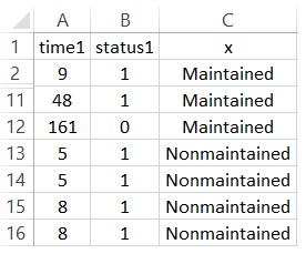
Figure 1: Structure of the CSV files for survival analysis (given by the aml data set).

The second corresponds to a data set from a clinical trial on colon cancer, which can be modeled using the progressive illness-death model [15]. Figure 2 shows the schematic diagram of transitions involved in the model. Among the variables of the colonIDM data set, the first four correspond to the times or the status indicator for the illness-death model. “time1” represents the sojourn time in the initial state and “Stime” and “event1” and “event” the corresponding censoring indicates. The other variables could be used for transition probabilities or to check the effect on the transition intensities (Figure 3).

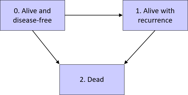
Figure 2: Illness-death model for the colon cancer study.

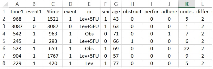
Figure 3: Structure of the CSV files for Illness-death models analysis (given by the colonIDM data set).

Finally, extensions to progressive processes beyond the three-state illness-death model are discussed using data from the European Group for Blood and Marrow Transplantation (EBMT) [4]. The movement of the patients among the six states can be modelled through the multi-state model with the following six states: ‘Alive and in remission, no recovery or adverse event’ (State 0); ‘Alive in remission, recovered from the treatment’ (state 1); ‘Alive in remission, occurrence of the adverse event’ (state 2); ‘Alive, both recovered and adverse event’ (state 3); ‘Alive, in relapse’ (treatment failure) (state 4) and ‘Dead (treatment failure)’ (state 5). In total there are 12 transitions, three intermediate events given by recovery (Rec), adverse event (AE) and a combination of the two (AE and Rec), and two absorbing states: Relapse and Death (Figure 4).

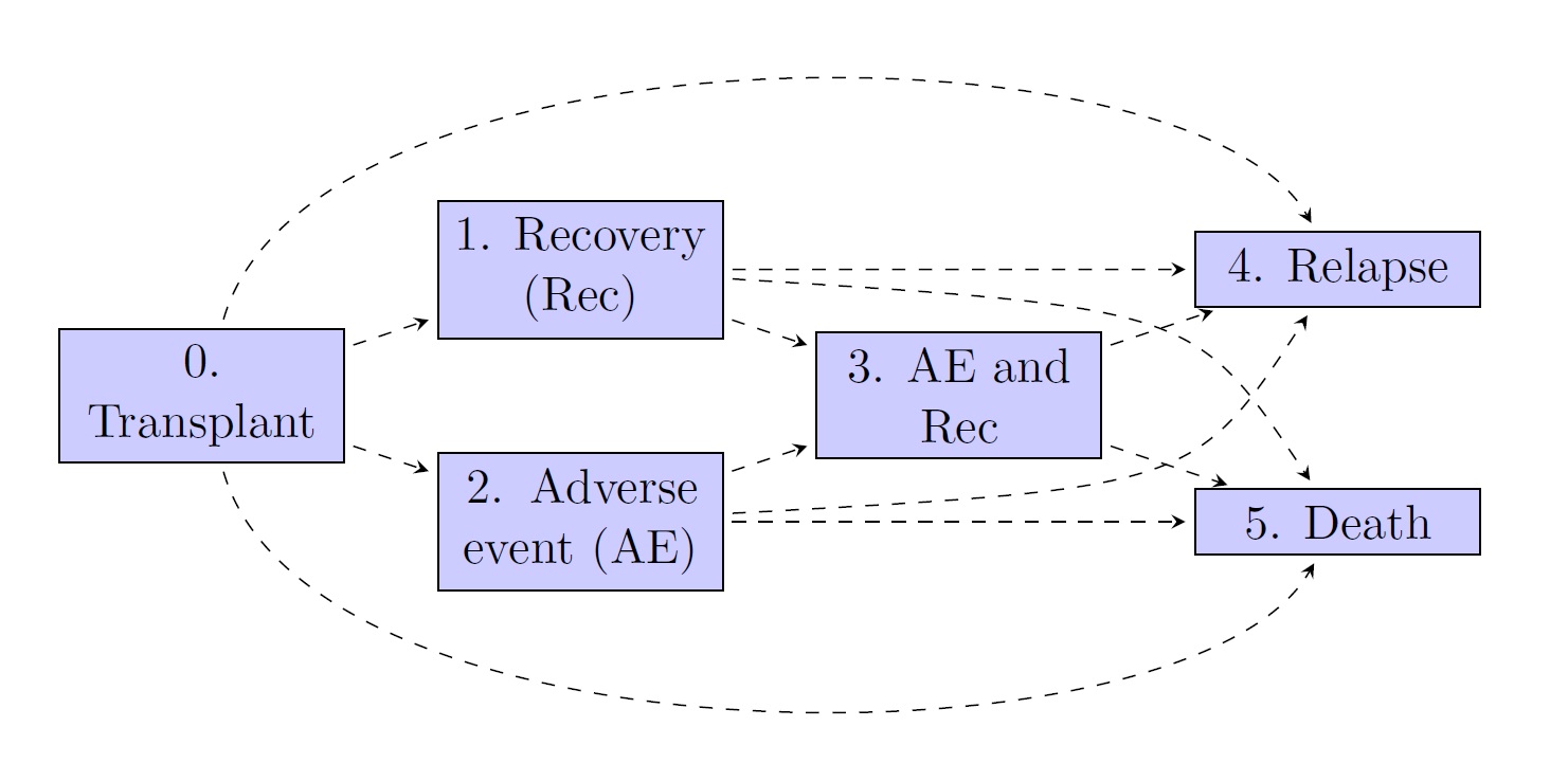
Figure 4: A six-states model for leukemia patients after bone marrow transplantation.

In terms of format, the CSV file should be in wide format. In the case of the ebmt4 data (Figure 5), the transition times from the initial to the ultimate state (‘srv’) or to the intermediate states (‘rec’, ‘ae’, ‘recae’ and ‘rel’), and the corresponding censoring variables are rec.s’, ‘ae.s’, ‘recae.s’, ‘rel.s’ and ‘srv.s’. Other variables correspond to the covariates for regression models.

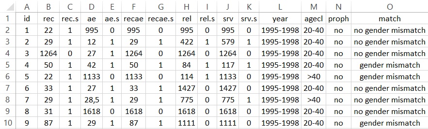
Figure 5: Structure of the CSV files for multi-state models analysis (given by the ebmt4 data set).

For all these data sets, the names of the variables could be different. In these cases, the user must correctly indicate the corresponding name in the web forms of the application. The data files can be accessed at https://w3.math.uminho.pt/~lmachado/shiny/.

7. How to select the input files?

On the “input files” page we can find an interactive form. For each type of data set (“survival data”, “illness-death model”, or “multi-state model”), a new web form appears below the radio buttons, in which we indicate the times to the events or the status indicator (Figure 6, left hand side and center). In case of the more complex multi-state models, it is also necessary to indicate the transition schema as well as the number of states, for instance (Figure 6, right hand side).

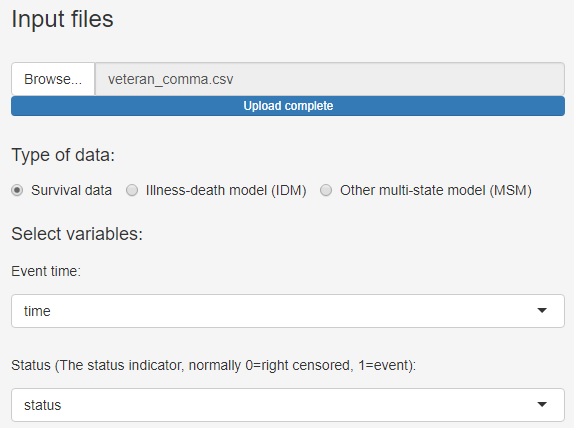
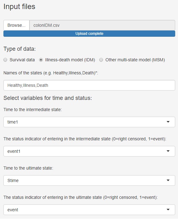
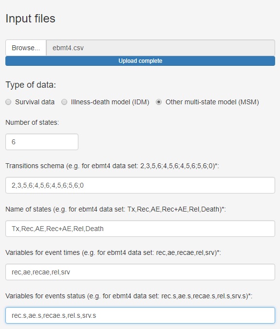
Figure 6: The event time and status variables for the survival analysis from the veteran data set (left); an indication of the two event times and their corresponding status for the illness-death model given by the colonIDM data (center); and a description of the MSM model through the number and the state names, the transition schema, and the event times and corresponding status for the ebmt4 data (right).

After submitting a data set, a table appears on the right hand side of the page which can be dynamically. This table can be changed using filters or by searching for specific words in the table. Figure 7 shows a partial view the veteran data set that can be found in the survival package.

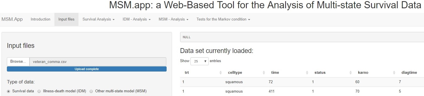
Figure 7: The input file page with the data table with some results for the veteran data set and three radio buttons for each type of model.

8. How to carry out a Survival analysis?

From the “survival analysis” button, we can carry out the classical methods for survival analysis. In this section, we analyze the main aspects of the outputs displayed on the right sides of the pages: Kaplan-Meier estimator, Compare survival curves, Cox PH models and parametric models, by using the veteran data set.

Kaplan-Meier estimator

Non-parametric estimation of the survival function is traditionally performed using the Kaplan-Meier estimator, which can be desegregated for different groups of categorical variables. By default, a summary of the estimates is presented on the right side. Figure 8 shows, respectively, times with events, the number of individuals at risk at that time, and the survival estimates with corresponding standard errors and confidence intervals. It is also possible to display an interactive plot of the survivals with (or without) the confidence interval intervals (Figure 9).

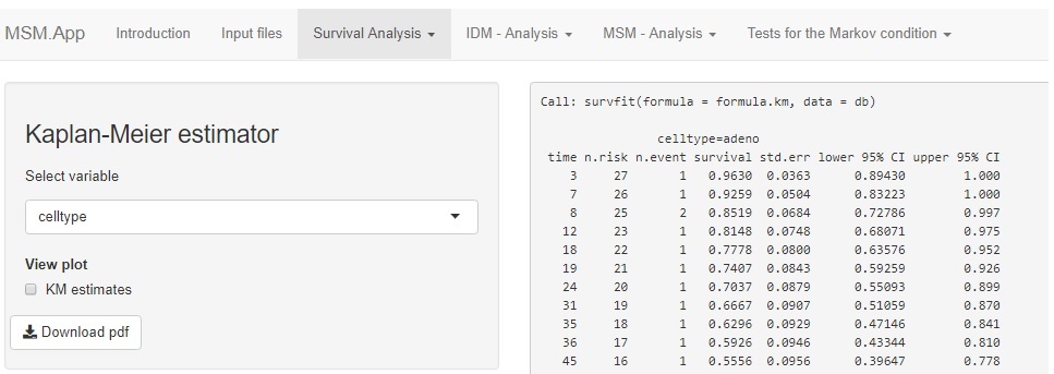
Figure 8: Summary of the survival estimation for the categorical covariate “celltype” of the veteran data set using the Kaplan-Meier estimator.

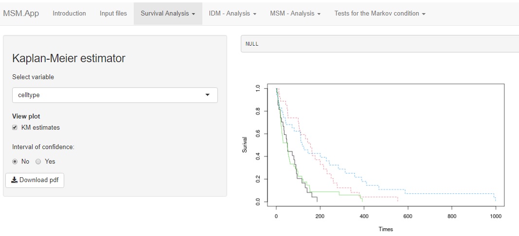
Figure 9: The output of the survival estimation for the categorical covariate “celltype” of the veteran data set using the Kaplan-Meier estimator. Survival curves for each group with confidence intervals could be shown at the bottom by choosing “Yes”.

Compare survival curves

Statistical tests can be used to compare survival rates between groups. The null hypothesis states that there is no difference in survival between groups. The log-rank test and the Gehan-Wilcoxon test are the most commonly used. Both tests are available in the MSM.App. The output of the tests comprises the chi-squared statistics, degrees of freedom, and the corresponding p-value. The number of individuals for each group and the number of observed and expected values are also presented. Results of Figure 10 show significant differences in the survival curves among groups given by the cell types ($p<$0.0001).

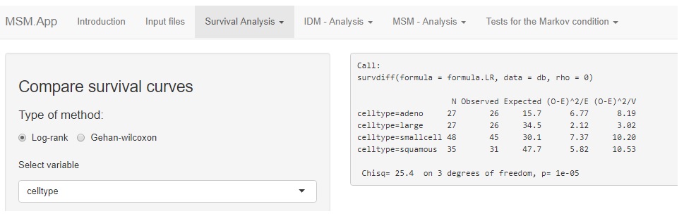
Figure 10: The output of the Log-rank test for the categorical covariate “celltype” of the veteran data set for testing the null hypothesis of no difference in survival between the two groups.

Cox PH models The semi-parametric Cox proportional hazards model [16] is usually used to evaluate the effects of several factors on survival. The output for the Cox model is updated as the user selects the variables to be included in the model in the web form. Figure 11 shows, respectively, the estimate of the coefficients for the covariates “celltype”, Karnofsky performance score (“karno”) and “age”; the hazard ratio given by $exp(coef)$ and the respective standard error; and the statistical significance of the model. Result of the global test for the proportional hazards assumption confirms that this requirement is no fulfilled and consequently a parametric accelerated failure time (AFT) model must be preferable to be fitted to this survival data.

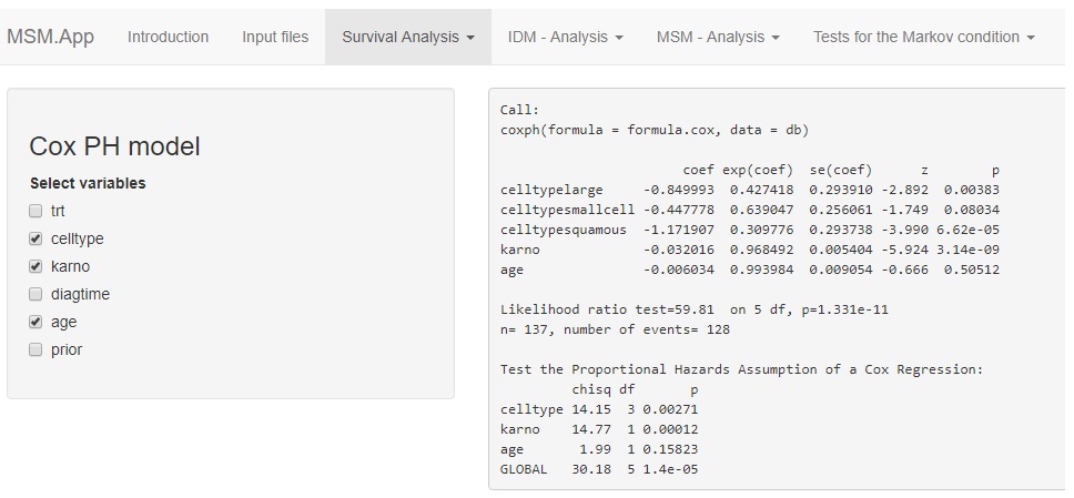
Figure 11: Results of the Cox model for the variables “celltype”, “karno” and “age” of the veteran data set. Result of the test for the proportional hazard assumption shows that a Cox PH model

Parametric AFT models The idea behind the outputs for parametric survival models is quite similar to those provided by the Cox PH models. In this case, six possibilities of distributions are available to model the baseline hazard function of the models: exponential, weibull, gaussian, logistic, lognormal or loglogistic. Besides the summary of the models, the Akaike Information Criterion (AIC) values are also presented to make it easier to compare which model fits better to assess the effect of several risk factors on survival time. Figures 12, 13 and 14 show, respectively, the outputs of the AFT models given by the exponential, weibull and loglogistic distributions. Through the AUC values we can assume that loglogistic parametric model is preferable. From this model, we can observe that only “age” and “small cells” do not have a significant effect on survival.

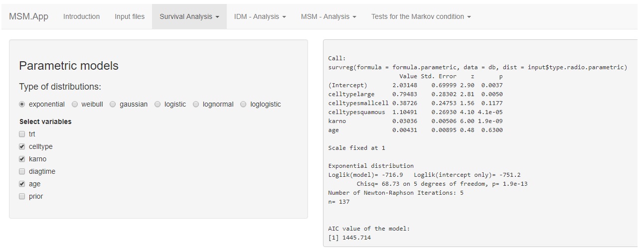
Figure 12: The outputs of the parametric models page with the results of the fitted model for the variables “celltype”, “karno” and “age” of the veteran data set using the exponential distribution.

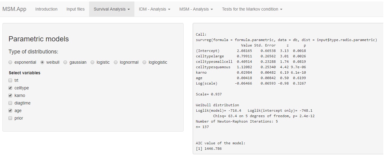
Figure 13: The outputs of the parametric models page with the results of the fitted model for the variables “celltype”, “karno” and “age” of the veteran data set using the weibull distribution.

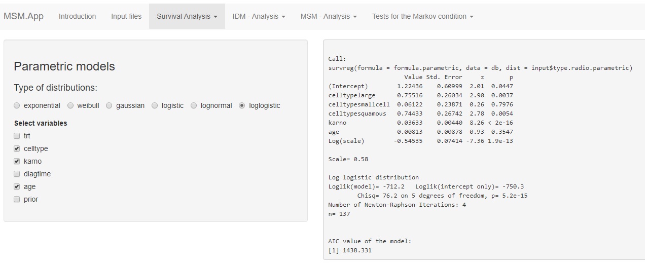
Figure 14: The outputs of the parametric models page with the results of the fitted model for the variables “celltype”, “karno” and “age” of the veteran data set using the loglogistic distribution.

9. How to carry out a illness-death model Analysis?

From the “ IDM-Analysis” button, we can carry out a data analysis of a progressive illness-death (IDM) model given by two events, three states, and three transitions. Number of events First, we are interested in having an idea of the movement of individuals among the three states. It is also possible to see the proportions of transitions (Figure 15).

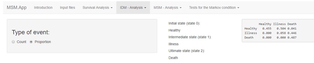
Figure 15: The number of transitions among the three states of the colonIDM data set.

Regression models In the multi-state models, there are so many transition intensities as there are transitions. For each one, we can then check the effect of the individual characteristics of the individuals by fitting separate intensities using semi-parametric Cox proportional hazard regression models [16]. In the inference of the regression models, we must take into account if the Markov condition, in which the past and future are independent given the present state, is verified. Regarding the dependence of the transition intensities and time, in the case of the failure of the markovianity, we can use a semi-Markov model in which the future of the process does not depend on the current time but rather on the duration of the current state. These two methods are available in MSM.app. In terms of interpretation, the outputs of the regression, for each transition, are very similar to those presented for the survival analysis. Results of Figures 16 indicate that save the treatment “Lev(amisole)+5-FU” all the other covariates have no effect for recurrence transition and only age could be considered important on mortality without recurrence. At least, only the covariates “perfor”, “sex” and the treatment “Obs” have no association for the transition from recurrence to mortality.

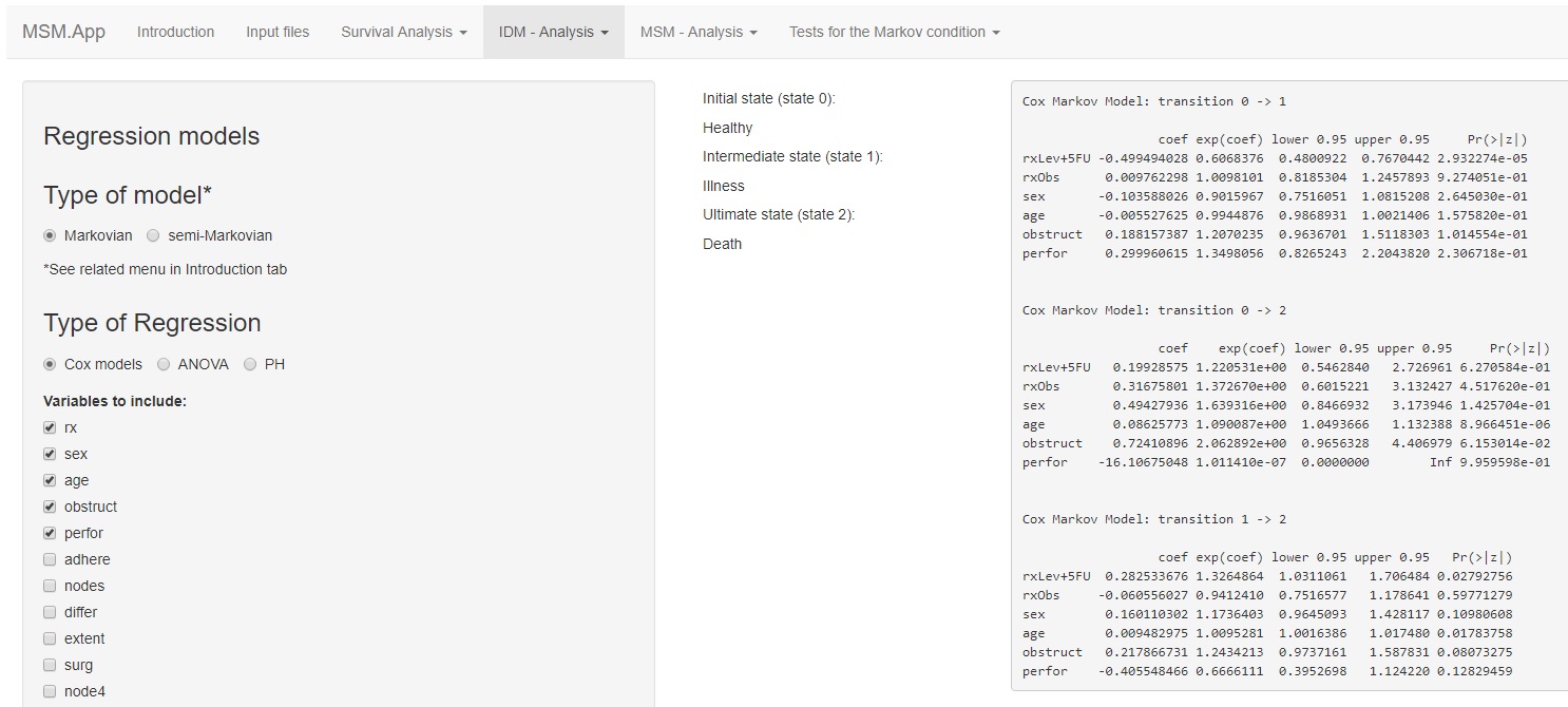
Figure 16: Results of the application of the Cox PH model with the following covariates: “rx”, “sex”, “age”, “obstruct” and “perfor”. Results for each of the three transition intensities of the colonIDM. A Markovian process is assumed.

It is also possible to obtain the outputs of ANOVA tests and the p-values of the tests for nonlinearity. For both outputs, the summaries show the chi-squared statistics and the p-values. For ANOVA tests, the log-likelihood values for each parameter are also presented (Figures 17 and 18).

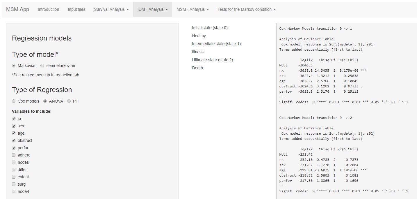
Figure 17: ANOVA results for transitions $0\longrightarrow 1$ and $0\longrightarrow 2$ with the following covariates: “rx”, “sex”, “age”, “obstruct” and “perfor” of the colonIDM. A Markovian process is assumed.

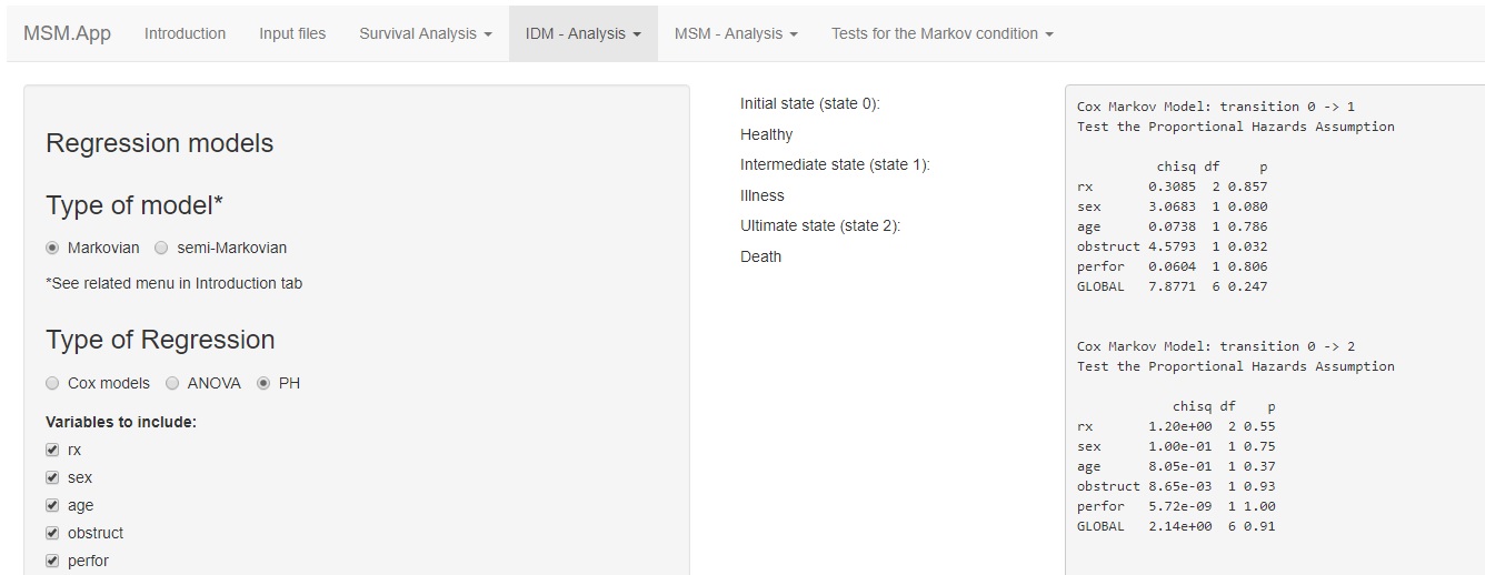
Figure 18: The proportional hazards assumption was tested for the transitions $0\rightarrow 1$ and $0\rightarrow 2$ with the following covariates: “rx”, “sex”, “age”, “obstruct” and “perfor” of the colonIDM. A Markovian process is assumed.

Transition probabilities The transition probabilities are quantities of particularly interest since they allow for long-term predictions of the multi-state process. The MSM.app allows estimating these quantities using the Aalen-Johansen estimator [17], the landmark methods (LM) proposed by [18], as well as its presmoothed version (PLM) proposed by [19], and the landmark Aalen-Johansen [20]. Related references can also be seen in the papers by [21] and [22]. Categorical covariates can be included using all four of these methods by splitting the sample for each level of the covariate and repeating the described procedures for each subsample. Through the IPCW estimator proposed by [23] is also possible to estimate transition probabilities conditional on one single continuous covariate. Finally, the MSM.app also provides the estimation of transition probabilities conditional on several covariates through Breslow’s method for estimating the baseline hazard function of the Cox models fitted marginally to each transition. The outputs for all these methods are identical. As an example, Figure 19 shows the estimates of the transition probabilities, using the landmark approach, from the initial single time $s=365$ days to the next four years (730, 1095, 1460, and 1825 days). Results are presented combining the values of the corresponding times and transitions which are labeled from “00” to “12”. For instance, “01” corresponds to the transition from the initial state (State 0) to intermediate state (Recurrence, State 1) and, in similar way, “12” the transition from the intermediate state (Recurrence, State 1) to death (State 2). Plots for each five transition probabilities are shown in Figure 20. $\widehat{p}_{00}(s=365,t)$ corresponds to the probability of a individual to occupy the initial state at time $t$ conditional to be in the same state at time $s=365$. In a similar way, $\widehat{p}_{11}(s,t)$ represents the conditional probability of those individuals observed in State 1 at time $s=365$ to remain in the intermediate state at a later time $t$. Plots for these transition probabilities report, respectively, survival fractions along times among the individuals that belong to initial state and the intermediate state at time $s=365$, being represented by monotone non-increasing functions. Plots for $\widehat{p}_{02}(s,t)$, report one minus the survival fraction along time, among the individuals in the initial state at time $s$. In this case, the plot is given by a monotone non-decreasing function. Finally, plots for $\widehat{p}_{01}(s,t)$ allows for an inspection along time of the probability of being in State 1 for the individuals who belong to State 0 at time $s$. As expected the confidence bands become wider with greater lags times $t-s$. Finally, Figure 21 depict the estimates of the transition probabilities for individuals with covariate values (“rx”,“sex”, and “age”) as Obs,1,48, respectively.

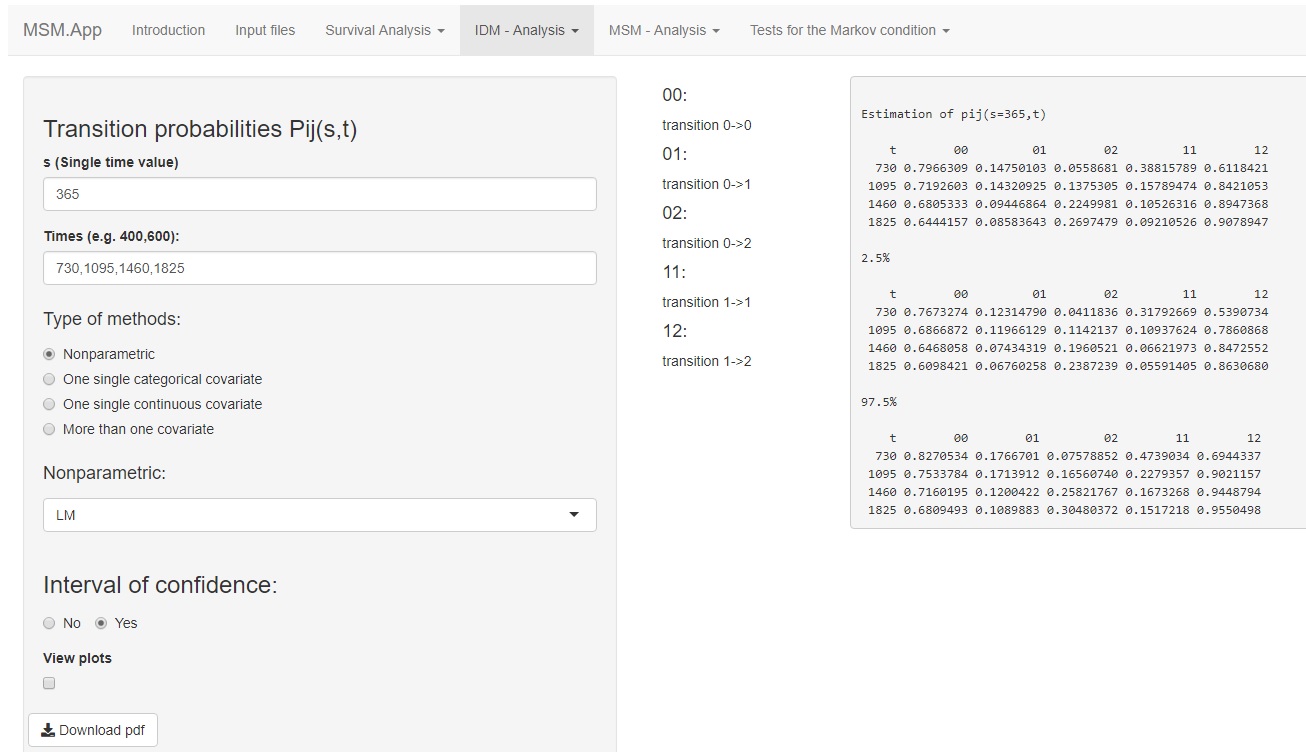
Figure 19: Results of the estimates of the transition probabilities and the corresponding confidence intervals for s = 365 and times 730, 1090, 1460, and 1825 days for the colonIDM data set using the landmark estimators.

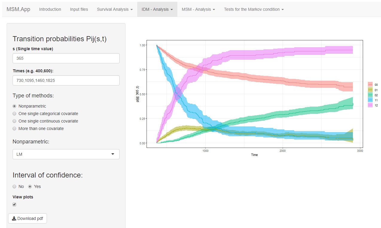
Figure 20: Transition probability estimates with confidence intervals for each transition for s = 365 using the landmark estimators.

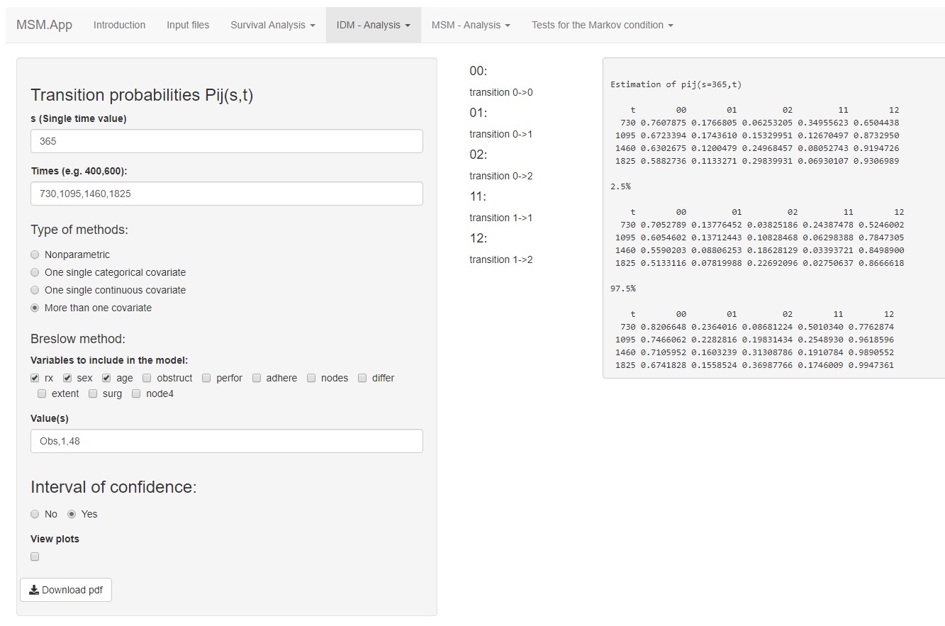
Figure 21: Results of the estimates of the transition probabilities and the corresponding confidence intervals for s = 365 and times 730, 1090, 1460, and 1825 days for the colonIDM data set using the Breslow estimator.

Cumulative Incidence Function (CIF) The cumulative incidence of the illness (intermediate state) is another quantity of interest in IDM models [24]. This quantity denotes the probability of the individual or item being or having been in the intermediate ‘diseased’ state at some particular time $t$. It can be estimated conditional on a covariate, continuous or categorical. Figure 22 shows the estimates, and respective bounds of confidence, of the CIF conditional to “age” at 50 years for three specific times.

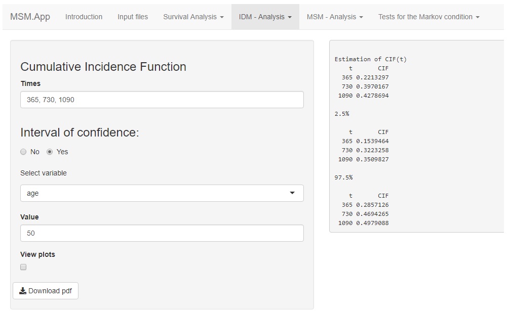
Figure 22: Cumulative recurrence incidence with 95% bootstrap confidence intervals. Data from a colon cancer study.

10. How to carry out a multi-state analysis for other models?

By clicking on the “MSM-analysis”, we can extend some of the methods addressed for the IDM models to more complex multi-state models (MSM) with more than three states and possible reversible transitions. Number of events Figure 23 shows the movement of the individuals among the six states of the multi-state model represented by the data set of the European Group for Blood and Marrow Transplantation (ebmt4 data set).

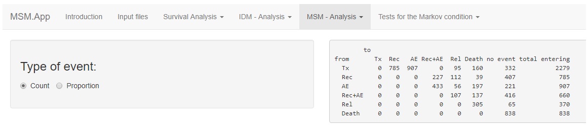
Figure 23: The number of transitions among the states of the ebmt4 data set.

Regression models Figure 24 shows the results of the Cox regression model for the transition $1\rightarrow 2$ which includes the covariates “year”, “age” and “proph”. As we can see, in terms of interpretation, the output is quite similar to those of IDM models but also shows the global significance of the model through different tests.

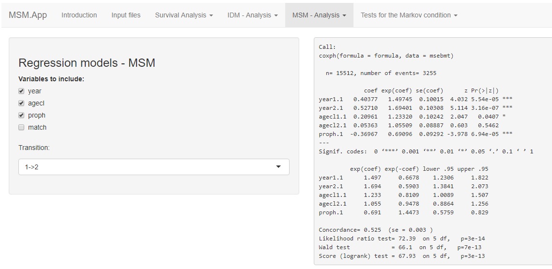
Figure 24: The output of the Cox regression model for the transition $1\rightarrow 2$ that include the ‘year”, “age” and “proph” covariates. ebmt4 data set.

Transition probabilities The steps for obtaining the transition probabilities are identical to those used for the illness-death model. In Figure 25, the output shows all the estimates from the indicated start and last states of the transition probabilities as well as the corresponding confidence intervals. A plot with the transition probability can also be presented for each transition.

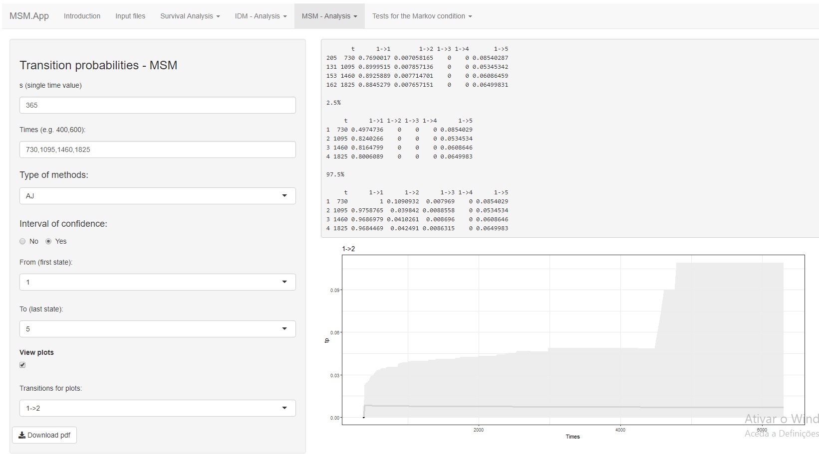
Figure 25: Estimates of all possible transition probabilities from the state 1 to 5, for s = 365 and times equal to 730, 1095, 1460, and 1825 using the AJ estimators. ebmt4 data set.

11. How to check the Markov condition?

Traditionally the Markov assumption is checked by including covariates depending on the history through a proportional hazards model. Since the landmark methods of the transition probabilities are free of the Markov assumption, they can also be used to introduce such tests by measuring their discrepancy to Markovian (AJ) estimators.

The MSM.app web application offers two types of tests for checking this assumption using recent literature methods: (i) local tests, which are obtained by fixing a specific time value, $s$ and are particularly useful for estimating transition probabilities; and (ii) global tests, which may be preferable for regression purposes.

Local tests

Two types of methods are available for checking the local tests of the Markov condition: (i) the AUC method, which is based on measuring the discrepancy between the AJ estimator of the transition probabilities (which provides consistent estimates when the process is Markovian) and the landmark estimators (which are free of the Markov condition). In this case, the web tool uses the LM estimator for the progressive illness-death models and LMAJ in the case of more complex MSM models; (ii) the Log-rank method, which considers summaries from families of log-rank statistics where patients are grouped by the state occupied at different times. For both types of models (IDM and MSM), the output using the AUC is the same. As an example, in Figure 26, we obtained the p-values for the local tests based on the $s$ times 365, 730, 1095, 1460, and 1825 for the transition from state 2 to state 3. Results were obtained for an IDM model based on the colon cancer data using 100 replicas. Even though the web form is quite similar to the AUC local test, the output of the log-rank test only provides the results for a specific transition and the times chosen (Figure 27).

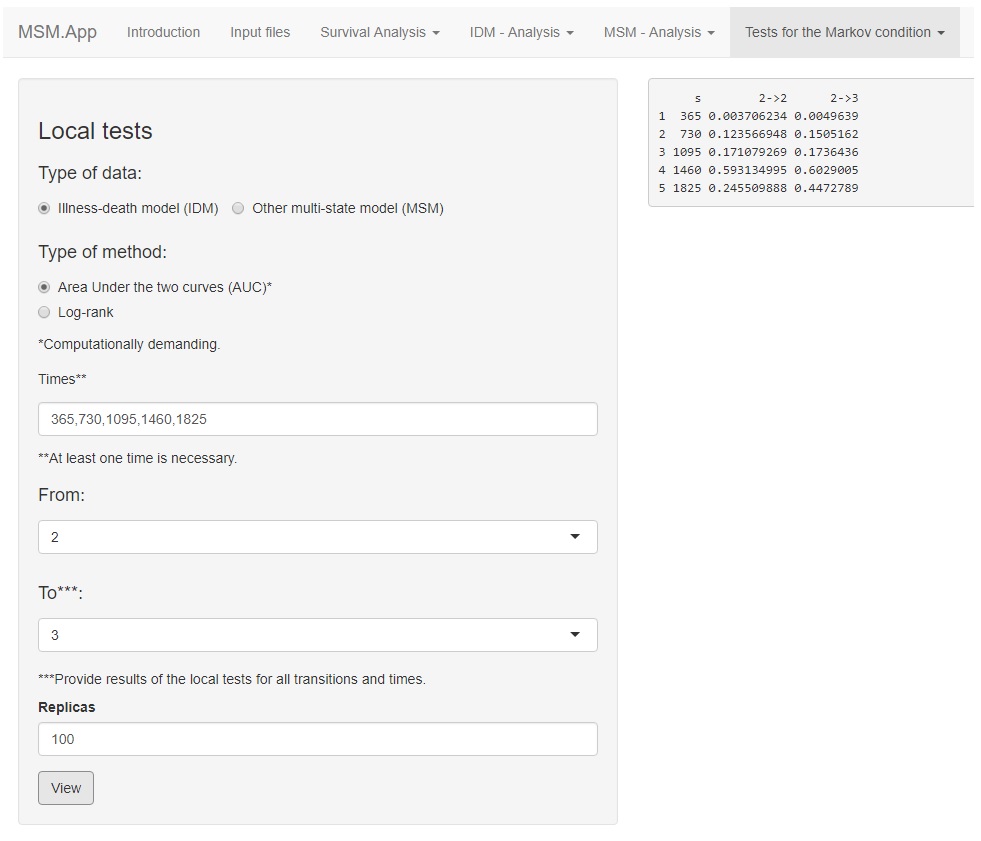
Figure 26: Results of the local test for the illness-death model using the colon cancer data set, for s = 365, 730, 1095, 1460, and 1825 days, using the AUC test, from state 1 to state 3.

Figure 27: Results of the local test for the illness-death model using the colon cancer data set, for s = 365, 730 and 1460 days, using the Log-rank test, for state 2 to state 3.

Global tests

In the MSM.app application, three global tests are available for both IMD and more complex MSM models: (i) the first one is based on Cox models, from which it is possible to evaluate the effect of history on the process. In this case, this can be done by checking the significance of the covariate time until entering the first state of a particular transition. As illustrated in Figure 28, we can conclude that there is no effect of the time spent in the initial state on the transition $2\rightarrow 3$ (p-value = 0.1543195), which does not induce the failure of the Markovianity. (ii) the recent proposed global test propose [25], based on the area under the curves (AUC), can be used. This test is based on the (AUC) local test results for specific percentiles. The outputs on the right hand of Figure 29 shows the proportion of rejections of the test for all possible transitions between state 1 and state 5. (iii) it is also possible to use the global test based on the log-rank statistics [26] throughout the similar steps of the previous methods, after selecting Log-rank in the radio button HTML element. The outputs provide only the results of the tests for each transition (Figure 30).

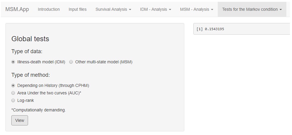
Figure 28: Results for this global test given by the Cox PH model to our data indicated that the effect of the time spent in State 1 is not significant (p-value of 0.154), revealing no evidence against the Markov model for the colon data set.

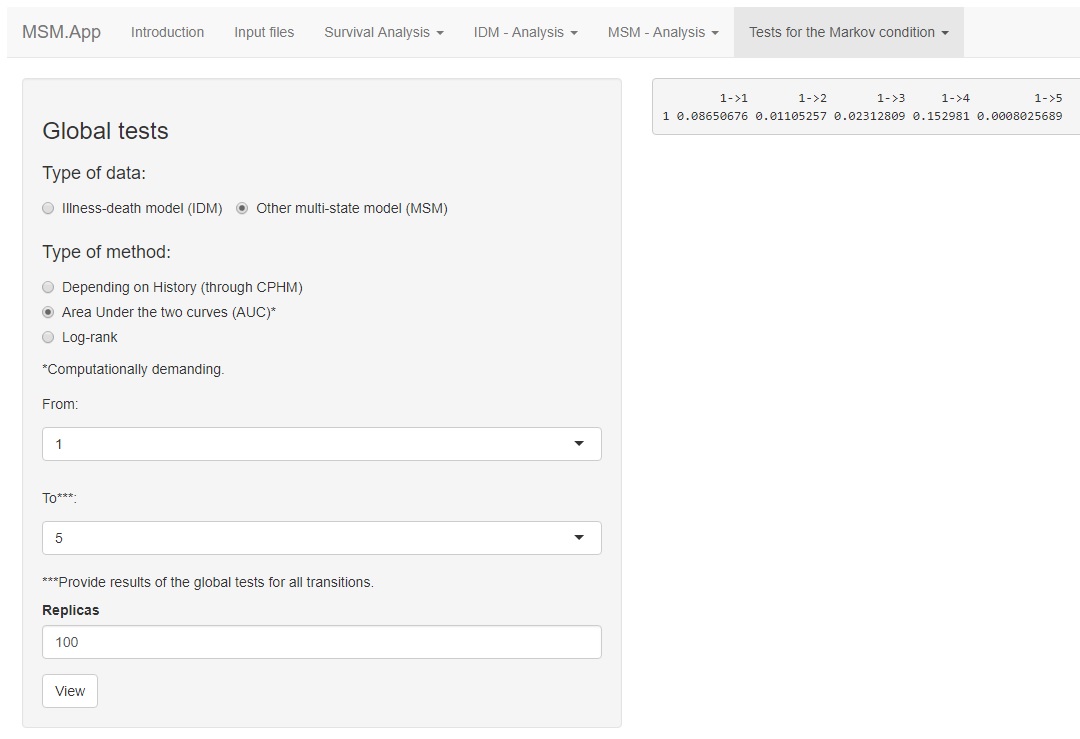
Figure 29: Outputs of the global test for the illness-death model based on the ebmt data set using the AUC test, from state 1 to state 5. Results for the AUC local test are also shown.

Figure 30: Results of the global test for the illness-death model using the colon cancer data set using the Log-rank test.

Acknowledgements

This research was financed within the research grants PTDC/MAT-STA /28248/2017 and PD/BD/142887/2018.

References

- [1] Wojciechowski, J., Hopkins, A. and Upton, R. Interactive pharmacometric applications using R and the Shiny package. CPT: pharmacometrics & systems pharmacology, 4(3), 146–159; 2015
- [2] Chang, W. Web Application Framework for R, CRAN; 2017
- [3] Kaushik, S. Creating Interactive data visualization using Shiny App in R (with examples), Analytics Vidhya; 2016
- [4] Putter, H., Fiocco, M. and Geskus, R.B. Tutorial in biostatistics: Competing risks and multi-state models, Statistics in Medicine, 26(11), 2389–2430.
- [5] Meira-Machado, L., de Uña-Álvarez, J. and Cadarso-Suárez, C. and Andersen, P.K. Multi-state models for the analysis of time to event data. Statistical Methods in Medical Research, 18, 195–222; 2009.
- [6] Meira-Machado, L. and Sestelo, M. Estimation in the progressive illness-death model: A nonexhaustive review. Biometrical Journal, 61 (2), 245–263; 2019.
- [7] Therneau, T.M. A Package for Survival Analysis in R. https://CRAN.R-project.org/ package=survival; 2021.
- [8] Putter, H., de Wreede, L.C., Fiocco, M., Geskus, R.B., Bonneville, E.F., Manevski, D. mstate: Data Preparation, Estimation and Prediction in Multi-State Models. The R Journal; 2020.
- [9] Soutinho, G., Sestelo, M. and Meira-Machado, L. survidm: An R package for Inference and Prediction in an Illness-Death Model. The R Journal, Accept for publication; 2021.
- [10] Govan, P. eAnalytics: Dynamic Web-based Analytics for the Energy Industry. Journal of Open Research Software, 4: e45; 2016. DOI: http://dx.doi.org/10.5334/jors.144
- [11] Seal, A., Wild, D.J. Netpredictor: R and Shiny package to perform Drug-Target Bipartite network analysis and prediction of missing links. Cold Spring Harbor Laboratory; 2016. doi: https://doi.org/10.1101/080036
- [12] Lacy, S. msm-shiny, https://stulacy.shinyapps.io/msm-shiny/; 2021
- [13] Skourlis, N., Crowther, M.J., Andersson , T., Lambert, P.C. MSMplus, https://nskbiostatistics.shinyapps.io/MSMplus/; 2021
- [14] Miller, R.G. Survival Analysis. John Wiley & Sons; 1997
- [15] Moertel, G., Fleming, T.R., Macdonald, J.S., Haller, D.G., Laurie, J.A., Goodman, P.J., Ungerleider, J.S., Emerson, W.A., Tormey, D.C., Glick, J.H., Veeder, M.H. and Mailliard, J.A., Levamisole and fluorouracil for adjuvant therapy of resected colon carcinoma. New England Journal of Medicine, 322(6):352–358; 1990
- [16] Cox, D.R. Regression models and life tables. Journal of the Royal Statistical Society Series B, 34, 187–220; 1972.
- [17] Aalen, O., Johansen, S. An empirical transition matrix for non homogeneous Markov and chains based on censored observations. Scandinavian Journal of Statistics, 5: 141–150; 1978.
- [18] de Uña-Álvarez, J. and Meira-Machado, L. Nonparametric estimation of transition probabilities in the non-markov illness-death model: A comparative study. Biometrics, 71(2), 364–375; 2015.
- [19] Meira-Machado, L. Smoothed landmark estimators of the transition probabilities. SORT-Statistics and Operations Research Transactions, 40: 375–398; 2016.
- [20] Putter, H. and Spitoni, C. Non-parametric estimation of transition probabilities in non-markov multistate models: The landmark aalen-johansen estimator. Statistical Methods in Medical Research, 27, 2081–2092; 2018.
- [21] Moreira, A., de Uña-Álvarez, J. and Meira-Machado, L. Presmoothing the aalen-johansen estimator inthe illness-death model. Electronical Journal of Statistics; 2013, 7:1491–1516. DOI: https://doi.org/10.1214/13-EJS816.
- [22] Araújo A, Meira-Machado L, Roca-Pardiñas J (2014). “TPmsm: Estimation of the Transition Probabilities in 3-State Models.” Journal of Statistical Software, 62(4), 1–29. doi: 10.18637/jss.v062.i04.
- [23] Meira-Machado, L., de Uña-Álvarez, J. and Datta, S. Nonparametric estimation of conditional transition probabilities in a non-Markov illness-death model. Computational Statistics, 2015, 30(2), 377–397. doi: https://doi.org/10.1007/s00180-014-0538-6
- [24] Kalbfleisch, J. D. and Prentice R. L. The statistical analysis of failure time data. John Wiley & Sons; 1980.
- [25] Soutinho, G. and Meira-Machado, L. Methods for checking the Markov condition in multi-state survival data. Comput Stat; 2021. https://doi.org/10.1007/s00180-021-01139-7
- [26] Titman, A. and Putter, H. General tests of the Markov property in multi-state models. Biostatistics; 2020. doi:10.1093/biostatistics/kxaa030.