Generalizing Aggregation Functions in GNNs: High-Capacity GNNs via Nonlinear Neighborhood Aggregators

Abstract.

Graph neural networks (GNNs) have achieved great success in many graph learning tasks. The main aspect powering existing GNNs is the multi-layer network architecture to learn the nonlinear graph representations for the specific learning tasks. The core operation in GNNs is message propagation in which each node updates its representation by aggregating its neighbors’ representations. Existing GNNs mainly adopt either linear neighborhood aggregation (mean, sum) or max aggregator in their message propagation. (1) For linear aggregators, the whole nonlinearity and network’s capacity of GNNs are generally limited due to deeper GNNs usually suffer from over-smoothing issue. (2) For max aggregator, it usually fails to be aware of the detailed information of node representations within neighborhood. To overcome these issues, we re-think the message propagation mechanism in GNNs and aim to develop the general nonlinear aggregators for neighborhood information aggregation in GNNs. One main aspect of our proposed nonlinear aggregators is that they provide the optimally balanced aggregators between max and mean/sum aggregations. Thus, our aggregators can inherit both (i) high nonlinearity that increases network’s capacity and (ii) detail-sensitivity that preserves the detailed information of representations together in GNNs’ message propagation. Promising experiments on several datasets show the effectiveness of the proposed nonlinear aggregators.

1. Introduction

Graph Neural Networks (GNNs) have achieved great success in many graph data representation and learning tasks, such as semi-supervised learning, clustering, graph classification etc. As we know that the main aspect powering existing GNNs is the multi-layer network architecture to learn the rich nonlinear graph representations for the specific learning tasks.

It is known that the core message propagation mechanism in multi-layer GNNs is neighborhood information aggregation in which each node is updated by aggregating the information from its neighbors. Most of existing GNNs generally adopt either linear neighborhood aggregation (e.g., mean, sum) (Kipf and Welling, 2017; Xu et al., 2019) or max aggregation (Hamilton et al., 2017) or combination of them (Dehmamy et al., 2019; Corso et al., 2020) in their layer-wise message propagation. For example, Kipf et al. (Kipf and Welling, 2017) present Graph Convolutional Networks (GCN) which adopts a weighted summation operation as the aggregation function. Veličković et al. (Veličković et al., 2018) present Graph Attention Networks (GAT) which uses a learned weighted mean aggregator via a self-attention mechanism. Hamilton et al. (Hamilton et al., 2017) propose the general GraphSAGE that employs mean, sum and max operation respectively for neighborhood aggregation. Dehmamy et al. (Dehmamy et al., 2019) propose a modular GCN design by combining different neighborhood aggregation rules (mean, sum, normalized mean) together with residual connections. Xu et al. (Xu et al., 2019) propose Graph Isomorphism Networks (GIN) in which the summation operation is utilized for neighborhood information aggregation for graph classification task. Geisler et al. (Geisler et al., 2020) propose reliable GNN by developing a robust aggregation function based on robust statistics in which the robust aggregator is implemented via an adaptively weighted mean aggregation function. Gabriele et al. (Corso et al., 2020) propose Principal Neighbourhood Aggregation (PNA) by integrating multiple aggregators (e.g., mean, max, min) together via degree-scalers. Cai et al. (Cai et al., 2021) propose Graph Neural Architecture Search (GNAS) to learn the optimal depth of message passing with max and sum neighbor aggregations.

After reviewing the previous GNNs on various graph learning tasks, we can find the following aspects. First, most of existing GNNs generally adopt linear aggregation functions as neighborhood information aggregators in their layer-wise message propagation, i.e., they learn the context-aware representation of each node by linearly aggregating the information from its neighbors. Thus, the whole nonlinearity of these linear aggregator based GNNs is determined based on the number of hidden layers (depth of networks). However, it is known that, deeper GNNs usually lead to over-smoothing issue (Kipf and Welling, 2017; Li et al., 2018; Zhao and Akoglu, 2020). Therefore, the whole nonlinearity and network’s capacity of these GNNs are generally limited. Second, the nonlinear max aggregator has been utilized in some works (Hamilton et al., 2017; Lee et al., 2017; Xu et al., 2019). As we know, max aggregator obviously fails to preserve the detailed information of node representations within each node’s neighborhood. Third, some recent works attempt to combine mean/sum and max aggregators together to provide a combined aggregator (Corso et al., 2020). However, the combined aggregator is explicitly depended on the individual mean/sum and max aggregators.

To address these issues, in this work, we re-think the message aggregation mechanism in layer-wise propagation of GNNs and aim to fully exploit the flexible nonlinear aggregation functions for information aggregation in GNNs. Specifically, we develop three kinds of non-linear neighborhood aggregators for GNNs’ message propagation by exploiting $L_{p}$-norm, polynomial and softmax functions respectively. Overall, there are three main aspects of the proposed methods. First, one important property of the proposed nonlinear neighborhood aggregators is that they can be regarded as intermediates between linear mean/summation and nonlinear max aggregators and provide the optimal flexible balanced aggregation strategies for GNNs. Thus, our aggregation mechanisms can inherit both (i) nonlinearity that increases network’s functional complexity/capacity and (ii) detail-sensitivity that preserves the detailed information of representations in GNNs’ message propagation. Second, the proposed aggregators are all differentiable that allow end-to-end training. Third, our aggregation mechanisms are general scheme which can integrate with many GNN architectures to enhance existing GNNs’ capacities and learning performance. Overall, we summarize the main contributions as follows:

• We propose to develop three kinds of nonlinear neighborhood aggregation schemes for the general GNNs’ layer-wise propagation.

• We analyze the main properties of the proposed nonlinear neighborhood aggregators and show the balanced behavior of the proposed models.

• We incorporate the proposed nonlinear aggregation mechanisms into GNNs and propose several novel networks for graph data representation and learning tasks.

We integrate our nonlinear aggregators into several GNN architectures and experiments on several datasets show the effectiveness of the proposed aggregators.

2. Revisiting Neighborhood Aggregation in GNNs

GNN provides a multi-layer network architecture for graph data representation and learning. It is known that the core operation of GNNs is the neighborhood aggregation for network’s layer-wise message propagation. Let $G(\mathbf{A},\mathbf{H})$ be the input graph where $\mathbf{A}\in\mathbb{R}^{n\times n}$ denotes the adjacency matrix and $\mathbf{H}=(\mathbf{H}_{1},\mathbf{H}_{2}\cdots\mathbf{H}_{n})\in\mathbb{R}^{n\times d}$ denotes the collection of node features. The neighborhood aggregation for layer-wise message propagation in GNNs (Hamilton et al., 2017; Geisler et al., 2020) can generally be formulated as follows,

(1) $$\mathbf{H}_{v}^{\prime}=\sigma\Big{(}\mathbf{W}\cdot\mathrm{AGG}\big{(}\mathbf{A}_{vu},\mathbf{H}_{u},{u}\in\mathcal{N}_{v}\big{)}\Big{)}$$

where $\mathcal{N}_{v}$ denotes the neighborhood of node $v$ (including node $v$) and matrix $\mathbf{W}$ denotes the layer-wise weight parameter. Function $\sigma(\cdot)$ denotes the activation function, such as $\mathrm{ReLU}$, $\mathrm{softmax}$, and $\mathrm{AGG}$ denotes the aggregation function, such as mean, summation, max, etc (Hamilton et al., 2017; Xu et al., 2019; Geisler et al., 2020).

For example, in Graph Convolutional Networks (GCN) (Kipf and Welling, 2017), it adopts the weighted summation aggregation over normalized graph in its layer-wise propagation as,

(2) $$\mathrm{AGG}\big{(}\mathbf{A}_{vu},\mathbf{H}_{u},{u}\in\mathcal{N}_{v}\big{)}=\sum_{u\in\mathcal{N}_{v}}\mathbf{\hat{A}}_{vu}\mathbf{H}_{u}$$

where $\hat{\mathbf{A}}=\tilde{\mathbf{D}}^{-\frac{1}{2}}\tilde{\mathbf{A}}\tilde{\mathbf{D}}^{-\frac{1}{2}}$ denotes the normalized adjacency matrix in which $\tilde{\mathbf{A}}=\mathbf{A}+\mathbf{I}$ and $\tilde{\mathbf{D}}$ is the diagonal matrix with $\tilde{\mathbf{D}}_{vv}=\sum_{u}\tilde{\mathbf{A}}_{vu}$. In Graph Attention Network (GAT) (Veličković et al., 2018), it first computes the attention $\alpha_{vu}$ for each graph edge as,

(3) $$\mathbf{\alpha}_{vu}=\mathrm{softmax}_{G}\big{(}\varphi_{\theta}(\textbf{H}_{v}\textbf{W},\textbf{H}_{u}\textbf{W})\big{)}$$

where $\textbf{W}\in\mathbb{R}^{d\times{d}^{\prime}}$ denotes the layer-specific weight matrix and $\mathrm{softmax}_{G}$ denotes the softmax function defined on topological graph. The function $\varphi_{\theta}(\cdot)$ denotes the learnable metric function parameterized by $\theta$. The parameter $\theta$ is shared across different edges to achieve information communication. Based on the learned edge attention $\alpha_{vu}$, GAT then conducts the layer-wise information aggregation as,

(4) $$\mathrm{AGG}\big{(}\mathbf{A}_{vu},\mathbf{H}_{u},{u}\in\mathcal{N}_{v}\big{)}=\sum_{u\in\mathcal{N}_{v}}\mathbf{\alpha}_{vu}\textbf{H}_{u}$$

In GraphSAGE (Hamilton et al., 2017), it employs the max-pooling operation over the neighborhood and implements layer-wise message aggregation as follows

(5) $$\mathrm{AGG}\big{(}\mathbf{A}_{vu},\mathbf{H}_{u},{u}\in\mathcal{N}_{v}\big{)}=\mathop{\mathrm{missing}}{max}\big{(}\big{\{}\mathcal{F_{\theta}}(\mathbf{H}_{u}),u\in\mathcal{N}_{v}\big{\}}\big{)}$$

where the $\mathcal{F_{\theta}}(\cdot)$ denotes the fully-connected network with an activation function and learnable parameter $\theta$. The function $\mathrm{max}$ denotes the element-wise max operation which aggregates the dimension-wise maximum value of node’s neighbors.

3. The Proposed Method

Most of existing GNNs mainly obtain nonlinear representations via activation function $\sigma$, such as $\mathrm{ReLU}$, $\mathrm{softmax}$ etc, in their layer-wise message propagation. Therefore, the nonlinearity of the whole network is determined based on the number of hidden layers. However, it is known that, deeper GNNs usually lead to over-smoothing issue (Kipf and Welling, 2017; Li et al., 2018; Zhao and Akoglu, 2020). Therefore, the nonlinearity and the whole learning capacity of existing GNNs are still limited. Besides, some GNNs use the nonlinear max aggregation as aggregator which fails to preserve the detailed information of node representations within each node’s neighborhood. To overcome these issues, we re-think the message aggregation mechanism in layer-wise propagation of GNNs and develop several nonlinear message aggregation functions to enhance the learning capacity of GNNs. To be specific, we propose three kinds of nonlinear aggregations, i.e., $L_{p}$-norm, polynomial and softmax aggregation. All these nonlinear aggregations provide balanced and self-adjust between mean and max functions, as discussed in detail below.

3.1. $L_{p}$-norm Aggregation

As a general nonlinear function, $L_{p}$-norm has been commonly used in computer vision and signal processing fields (Gulcehre et al., 2014; Estrach et al., 2014). Here, we propose to exploit $L_{p}$-norm function for the neighborhood aggregation in GNN’s layer-wise message propagation.

Given $G(\mathbf{A},\mathbf{H})$ be the input graph where $\mathbf{A}\in\mathbb{R}^{n\times n}$ denotes the adjacency matrix and $\mathbf{H}=(\mathbf{H}_{1},\mathbf{H}_{2}\cdots\mathbf{H}_{n})\in\mathbb{R}^{n\times d}$ denotes the collection of node features. One straightforward way to adopt $L_{p}$-norm for the neighborhood aggregation can be formulated as

(6) $$\mathrm{AGG}_{\ell_{p}}\big{(}\mathbf{A}_{vu},\mathbf{H}_{u},{u}\in\mathcal{N}_{v}\big{)}=\Big{(}\sum_{u\in\mathcal{N}_{v}}\mathbf{{A}}_{vu}\big{|}\mathbf{H}_{u}\big{|}^{p}\Big{)}^{1/p}$$

Here, $\big{|}\mathbf{H}_{u}\big{|}^{p}\in\mathbb{R}^{d}$ is defined as

$$\big{|}\mathbf{H}_{u}\big{|}^{p}=\left(\big{|}\mathbf{H}_{u1}\big{|}^{p},\big{|}\mathbf{H}_{u1}\big{|}^{p}\cdots\big{|}\mathbf{H}_{u1}\big{|}^{p}\right)$$

where $p\in[1,+\infty)$ is a parameter which can be learned adaptively. However, the negative information has been ignored in Eq.(6). To address this issue, we adapt the above $L_{p}$-norm function and propose our aggregation as follows,

(7) $$\mathrm{AGG}_{\ell_{p}}=\Big{(}\sum_{u\in\mathcal{N}_{v}}\mathbf{{A}}_{vu}{\big{(}\mathbf{H}_{u}-\mu_{m}\big{)}}^{p}\Big{)}^{1/p}+{\mu}_{m}$$

where $\mu_{m}=\min_{u,k}\big{\{}\textbf{H}_{uk}\big{\}}$ denotes the minimum element of matrix H and $\textbf{H}_{u}\in\mathbb{R}^{d}$ denotes the feature vector of node $u$.

Remark. The proposed $\mathrm{AGG}_{\ell_{p}}$ is a general scheme which can be integrated with many GNN’ architectures, such as GCN (Kipf and Welling, 2017), GAT (Veličković et al., 2018), GraphSAGE (Hamilton et al., 2017), etc. For example, one can replace $\mathbf{{A}}_{vu}$ with ${\mathbf{\hat{A}}}_{vu}$ in Eq.(2) to produce a GCN variant (Kipf and Welling, 2017). Also, one can use the learned graph attention $\alpha_{vu}$ in Eq.(4) to replace $\mathbf{{A}}_{vu}$ to generate a new GAT model. In particular, one main property of the proposed $\mathrm{AGG}_{\ell_{p}}$ is that it provides a balanced aggregator between max aggregator and summation aggregator. Specifically, we have the following Proposition 1.

Proposition 1: When $p=1$, $\mathrm{AGG}_{\ell_{p}}$ becomes to the weighted summation aggregation; When $p\to\infty$, it is equivalent to the max aggregation.

Proof. When $p=1$, one can easily observe that $\mathrm{AGG}_{\ell_{p}}$ becomes to the weighted summation aggregation. For the case $p\to\infty$, we first prove the following conclusion.

To be specific, given any vector $x$ and $a\in\mathbb{R}^{n},a_{i}\geq 0$, without loss of generality, we assume $x_{m}$ be the unique maximum value of $x$. Below, we can show that

$$\lim_{p\to\infty}\Big{(}\sum^{n}_{i=1}a_{i}|x_{i}|^{p}\Big{)}^{1/p}=\lim_{p\to\infty}\Big{(}|x_{m}|^{p}\sum^{n}_{i=1}a_{i}\big{(}\frac{|x_{i}|}{|x_{m}|}\big{)}^{p}\Big{)}^{1/p}$$

(8) $$=|x_{m}|\lim_{p\to\infty}\Big{(}\sum^{n}_{i=1}a_{i}\big{(}\frac{|x_{i}|}{|x_{m}|}\big{)}^{p}\Big{)}^{1/p}$$

For any $i\neq m$, since $\frac{|x_{i}|}{|x_{m}|}<1$, thus $\lim_{p\to\infty}\big{(}\frac{|x_{i}|}{|x_{m}|}\big{)}^{p}=0$. Thus, we have

(9) $$|x_{m}|\lim_{p\to\infty}\Big{(}\sum^{n}_{i=1}a_{i}\big{(}\frac{|x_{i}|}{|x_{m}|}\big{)}^{p}\Big{)}^{1/p}=|x_{m}|\lim_{p\to\infty}\big{(}a_{m}\big{)}^{1/p}=|x_{m}|$$

Based on the above analysis, one can see that

(10) $$\lim_{p\to\infty}\Big{(}\sum_{u\in\mathcal{N}_{v}}\mathbf{{A}}_{vu}{(\mathbf{H}_{u}-\mu_{m})}^{p}\Big{)}^{1/p}+{\mu}_{m}=\max_{k\in\{1,2\cdots d\}}\big{\{}\textbf{H}_{uk}\big{\}}$$

This completes the proof.

3.2. Polynomial Aggregation

In addition to $L_{p}$-norm, we also explore polynomial function (Wei et al., 2019) for neighborhood information aggregation.

Given $G(\mathbf{A},\mathbf{H})$ be the input graph where $\mathbf{A}\in\mathbb{R}^{n\times n}$ denotes the adjacency matrix and $\mathbf{H}=(\mathbf{H}_{1},\mathbf{H}_{2}\cdots\mathbf{H}_{n})\in\mathbb{R}^{n\times d}$ denotes the node features. Formally, we propose to define polynomial aggregation $\mathrm{AGG}_{\mathcal{P}}$ as

(11) $$\mathrm{AGG}_{\mathcal{P}}\big{(}\mathbf{A}_{vu},\mathbf{H}_{u},{u}\in\mathcal{N}_{v}\big{)}=\dfrac{\sum\limits_{u\in\mathcal{N}_{v}}\mathbf{{A}}_{vu}|\mathbf{H}_{u}|^{\alpha+1}}{\sum\limits_{u\in\mathcal{N}_{v}}\mathbf{{A}}_{vu}|\mathbf{H}_{u}|^{\alpha}}$$

where the division operation in Eq.(11) is the element-wise division and $|\mathbf{H}_{u}|^{\alpha}\in\mathbb{R}^{d}$ is defined as

$$\big{|}\mathbf{H}_{u}\big{|}^{\alpha}=\big{(}\big{|}\mathbf{H}_{u1}\big{|}^{\alpha},{\big{|}\mathbf{H}_{u1}\big{|}}^{\alpha}\cdots\big{|}\mathbf{H}_{u1}\big{|}^{\alpha}\big{)}$$

where $\alpha\in[0,+\infty)$ is a parameter which controls its polynomial order. In this paper, the parameter value of $\alpha$ is learned adaptively. Similar to the above $L_{p}$-norm function, considering the inevitable negative elements in H and the power operation (Wei et al., 2019), we adapt the Eq.(11) and finally propose our $\mathrm{AGG}_{\mathcal{P}}$ as follows,

(12) $$\mathrm{AGG}_{\mathcal{P}}=\frac{\sum\limits_{u\in\mathcal{N}_{v}}\mathbf{{A}}_{vu}{\big{(}\mathbf{H}_{u}-\mu_{m}\big{)}}^{\alpha+1}}{\sum\limits_{u\in\mathcal{N}_{v}}\mathbf{{A}}_{vu}{\big{(}\mathbf{H}_{u}-\mu_{m}\big{)}}^{\alpha}}+\mu_{m}$$

where $\mu_{m}$ is the minimum element of H and the division operation is the element-wise division.

Similar to $\mathrm{AGG}_{\ell_{p}}$, $\mathrm{AGG}_{\mathcal{P}}$ also gives a general scheme and can be integrated with many GNNs’ architectures, such as GCN (Kipf and Welling, 2017), GAT (Veličković et al., 2018), GraphSAGE (Hamilton et al., 2017), etc. In addition, $\mathrm{AGG}_{\mathcal{P}}$ also provides a balanced aggregator between max and summation aggregator (Wei et al., 2019). Formally, we have the following Proposition 2.

Proposition 2: When $\alpha=0$, $\mathrm{AGG}_{\mathcal{P}}$ becomes to the weighted mean aggregation; When $\alpha\to+\infty$, it is equivalent to the max aggregation.

The mathematical proof of this Proposition 2 can be similarly obtained by referring to work (Wei et al., 2019).

3.3. Softmax Aggregation

The nonlinear function softmax has been commonly used as activity function in GNNs. Given a vector $x\in\mathbb{R}^{n}$, the standard softmax function is defined as follows,

(13) $$\mathrm{Softmax}(x)_{i}=\frac{{e}^{\gamma x_{i}}}{\sum\limits_{i=1}^{n}{e}^{\gamma x_{i}}},i=1,2\cdots n$$

where $\gamma>0$ is a scale factor. It is known that softmax is a smooth approximation of argmax function, i.e., let $x_{m}$ be the maximum value of $x$, then

(14) $$\lim_{\gamma\to+\infty}\mathrm{Softmax}(x)_{i}=\left\{\begin{aligned} &1,\,\,\,i=m\\ &0,\,\,\,otherwise\end{aligned}\right.$$

In our work, we exploit softmax function for neighborhood information aggregation in GNNs. To be specific, given $G(\mathbf{A},\mathbf{H})$ be the input graph where $\mathbf{A}\in\mathbb{R}^{n\times n}$ denotes the adjacency matrix and $\mathbf{H}=(\mathbf{H}_{1},\mathbf{H}_{2}\cdots\mathbf{H}_{n})\in\mathbb{R}^{n\times d}$ denotes the node features. Formally, our softmax based aggregator $\mathrm{AGG}_{\mathcal{S}}$ is defined as

(15) $$\mathrm{AGG}_{\mathcal{S}}=\sum_{u\in\mathcal{N}_{v}}\mathbf{{A}}_{vu}\Big{(}\textbf{H}_{u}\odot\frac{{e}^{\gamma\mathbf{H}_{u}}}{\sum\limits_{u\in\mathcal{N}_{v}}{e}^{\gamma\mathbf{H}_{u}}}\Big{)}$$

where $\gamma\in[0,+\infty)$ denotes the scalar parameter and $\odot$ indicates the element-wise product. $\mathbf{H}_{u}\in\mathbb{R}^{d}$ denotes the feature vector of node $u$. The division operation in Eq.(15) denotes the element-wise division. The operation $e^{\gamma\mathbf{H}_{u}}$ is defined as

$$e^{\gamma\mathbf{H}_{u}}=\big{(}e^{\gamma\mathbf{H}_{u1}},e^{\gamma\mathbf{H}_{u2}}\cdots e^{\gamma\mathbf{H}_{ud}}\big{)}$$

Similar to the above two nonlinear aggregators, $\mathrm{AGG}_{\mathcal{S}}$ can also combine with some GNNs’ architectures, such as GCN (Kipf and Welling, 2017) and GAT (Veličković et al., 2018), etc. In addition, we can show that $\mathrm{AGG}_{\mathcal{S}}$ provides an adaptive aggregator between max and mean aggregations. Formally, we have the following proposition.

Proposition 3: When $\gamma=0$, $\mathrm{AGG}_{\mathcal{S}}$ becomes to the weighted mean aggregation; When $\gamma\to\infty$, it is equivalent to the max aggregation.

When $\gamma=0$, $\mathrm{AGG}_{\mathcal{S}}$ obviously becomes to the weighted mean aggregator. For $\gamma\to\infty$, the proof can be easily obtained by using Eq.(14).

Table 1. The introduction and usage of experimental datasets.

Dataset	Cora	Citeseer	Pubmed	Amazon Photo	Amazon Computers	PPI
Nodes	2708	3327	19717	7487	13381	56944
Feature	1433	3703	500	745	767	50
Edges	5429	4732	44338	119043	245778	266144
Classes	7	6	3	8	10	121

Table 2. Results of semi-supervised classification for transductive learning task.

Method	Cora	Citeseer	Pubmed	Photo	Computers
GCN (baseline)	81.24$\pm$1.68	69.92$\pm$1.75	79.82$\pm$1.60	89.05$\pm$1.80	80.02$\pm$2.83
GCN-$\mathrm{AGG}_{\ell_{p}}$	82.57$\pm$1.88	71.03$\pm$0.74	80.72$\pm$1.00	90.86$\pm$1.06	81.98$\pm$2.27
GCN-$\mathrm{AGG}_{\mathcal{P}}$	82.20$\pm$1.60	71.12$\pm$1.10	81.01$\pm$1.29	91.80$\pm$0.50	82.86$\pm$1.41
GCN-$\mathrm{AGG}_{\mathcal{S}}$	83.10$\pm$1.28	71.50$\pm$1.12	81.50$\pm$0.82	91.25$\pm$0.80	82.02$\pm$2.11
Masked GCN (baseline)	81.44$\pm$1.19	69.10$\pm$1.98	80.19$\pm$1.40	88.60$\pm$3.08	76.06$\pm$7.09
Masked GCN-$\mathrm{AGG}_{\ell_{p}}$	82.56$\pm$1.45	69.96$\pm$1.33	80.92$\pm$1.18	90.56$\pm$1.19	80.63$\pm$4.92
Masked GCN-$\mathrm{AGG}_{\mathcal{P}}$	82.00$\pm$1.02	69.94$\pm$1.23	81.03$\pm$0.81	90.98$\pm$1.95	78.15$\pm$6.44
Masked GCN-$\mathrm{AGG}_{\mathcal{S}}$	82.88$\pm$1.00	70.10$\pm$1.04	81.50$\pm$1.06	90.57$\pm$1.56	81.50$\pm$2.75
GAT (baseline)	82.02$\pm$1.55	70.88$\pm$1.36	80.05$\pm$0.97	89.72$\pm$2.02	79.72$\pm$2.20
GAT-$\mathrm{AGG}_{\ell_{p}}$	83.22$\pm$0.78	72.24$\pm$0.99	80.49$\pm$1.14	90.37$\pm$2.10	81.14$\pm$1.80
GAT-$\mathrm{AGG}_{\mathcal{P}}$	83.30$\pm$1.15	71.56$\pm$1.46	80.29$\pm$1.05	90.70$\pm$1.49	82.60$\pm$1.62
GAT-$\mathrm{AGG}_{\mathcal{S}}$	83.14$\pm$1.30	72.15$\pm$1.01	81.05$\pm$1.22	90.65$\pm$2.10	81.26$\pm$2.10
CAT (baseline)	82.45$\pm$1.40	72.46$\pm$1.33	80.12$\pm$1.10	88.04$\pm$2.14	80.53$\pm$1.85
CAT-$\mathrm{AGG}_{\ell_{p}}$	82.93$\pm$1.30	72.50$\pm$0.87	81.52$\pm$1.28	90.54$\pm$1.08	81.10$\pm$1.92
CAT-$\mathrm{AGG}_{\mathcal{P}}$	82.60$\pm$1.45	71.78$\pm$1.15	81.35$\pm$1.91	90.65$\pm$0.81	82.66$\pm$1.43
CAT-$\mathrm{AGG}_{\mathcal{S}}$	83.34$\pm$1.41	72.61$\pm$0.80	82.04$\pm$1.40	91.21$\pm$0.66	82.90$\pm$1.98

4. Experiments

To validate the effectiveness of our proposed nonlinear aggregators, we take two GCN-based models (GCN (Kipf and Welling, 2017) and Masked GCN (Yang et al., 2019)) and two GAT-based models (GAT (Veličković et al., 2018) and CAT (He et al., 2021)) as baseline architectures and perform evaluations on several widely used graph learning datasets.

4.1. Experimental Settings

Dataset Setting. We test the proposed models on six datasets including Cora, Citeseer, Pubmed (Sen et al., 2008), PPI (Hamilton et al., 2017), Amazon Photo and Computers (Shchur et al., 2018). Similar to work (Kipf and Welling, 2017), we randomly select $20$ nodes per class as training set, $500$ nodes and $1000$ nodes as validation and testing set respectively. For Amazon Photo and Computers (Shchur et al., 2018), following work (Shchur et al., 2018), we randomly select $20$ nodes per class as training set, $30$ nodes per class and the remaining nodes as validation and testing set respectively. For PPI dataset, similar to the setting in work (Veličković et al., 2018), we take $20$ graphs as training set, $2$ graphs as validation set and $2$ graphs as testing set. The introduction and usage of these datasets are summarized in Table 1.

Parameter Setting. We integrate the proposed nonlinear aggregators with GCNs and GATs respectively. For GCN-based methods, the number of hidden layer units is selected from ${16,64}$ for all datasets. For GAT-based methods, the number of hidden layer units is set to $8$ on all datasets. The weight decay are set to $5e-4$ and $1e-5$ for citation and amazon datasets, respectively. Our network parameters $\{W,p/\alpha/\gamma\}$ are trained and optimized by gradient descent algorithms (Kingma and Ba, 2015; Qian, 1999).

Table 3. Results of semi-supervised clustering on five datasets.

Method	Cora	Citeseer	Pubmed	Photo	Computers
GCN (baseline)	80.24$\pm$0.97	70.15$\pm$0.60	79.10$\pm$1.22	89.00$\pm$1.45	80.36$\pm$2.40
GCN-$\mathrm{AGG}_{\ell_{p}}$	82.40$\pm$0.82	70.58$\pm$0.83	79.98$\pm$1.21	91.04$\pm$1.10	82.43$\pm$1.95
GCN-$\mathrm{AGG}_{\mathcal{P}}$	82.14$\pm$0.95	71.00$\pm$0.89	79.96$\pm$0.98	92.06$\pm$0.33	83.14$\pm$1.38
GCN-$\mathrm{AGG}_{\mathcal{S}}$	82.87$\pm$0.91	71.28$\pm$0.82	80.64$\pm$0.89	91.22$\pm$0.82	82.53$\pm$1.82
Masked GCN (baseline)	80.74$\pm$0.78	69.03$\pm$1.78	79.14$\pm$1.05	88.83$\pm$3.03	76.19$\pm$7.25
Masked GCN-$\mathrm{AGG}_{\ell_{p}}$	82.40$\pm$0.66	69.76$\pm$1.07	80.26$\pm$0.85	90.76$\pm$1.16	80.92$\pm$5.00
Masked GCN-$\mathrm{AGG}_{\mathcal{P}}$	81.90$\pm$0.42	69.83$\pm$1.02	80.00$\pm$1.06	91.15$\pm$1.90	78.74$\pm$6.28
Masked GCN-$\mathrm{AGG}_{\mathcal{S}}$	82.58$\pm$0.85	69.96$\pm$1.08	80.76$\pm$1.26	90.79$\pm$1.52	81.87$\pm$2.69
GAT (baseline)	82.55$\pm$0.40	71.02$\pm$0.30	80.01$\pm$0.71	88.55$\pm$0.70	78.98$\pm$1.20
GAT-$\mathrm{AGG}_{\ell_{p}}$	83.62$\pm$0.56	72.30$\pm$0.45	80.40$\pm$1.16	90.61$\pm$1.33	81.93$\pm$1.91
GAT-$\mathrm{AGG}_{\mathcal{P}}$	83.68$\pm$0.65	71.76$\pm$1.10	80.22$\pm$0.80	90.78$\pm$1.18	81.06$\pm$1.20
GAT-$\mathrm{AGG}_{\mathcal{S}}$	83.50$\pm$0.65	71.73$\pm$0.76	80.89$\pm$1.10	90.84$\pm$1.15	80.54$\pm$1.94
CAT (baseline)	81.98$\pm$1.01	70.35$\pm$0.72	77.85$\pm$3.48	89.67$\pm$1.16	80.55$\pm$1.69
CAT-$\mathrm{AGG}_{\ell_{p}}$	82.59$\pm$0.82	71.68$\pm$0.66	79.75$\pm$1.27	90.72$\pm$1.05	81.88$\pm$1.78
CAT-$\mathrm{AGG}_{\mathcal{P}}$	82.10$\pm$1.10	70.49$\pm$0.85	79.92$\pm$1.16	90.83$\pm$0.77	83.00$\pm$1.39
CAT-$\mathrm{AGG}_{\mathcal{S}}$	82.60$\pm$1.03	71.78$\pm$0.75	80.40$\pm$1.24	91.42$\pm$0.61	83.25$\pm$1.94

4.2. Comparison Results

Node Classification. We first test our proposed models on transductive learning task and take some popular GNNs as baselines including Graph Convolutional Network (GCN) (Kipf and Welling, 2017), Graph Attention Networks (GAT) (Veličković et al., 2018), Masked GCN (Yang et al., 2019) and CAT (He et al., 2021). Table 2 reports the comparison results. One can observe that the proposed nonlinear aggregators can consistently improve the baseline models which demonstrates the effectiveness of our proposed nonlinear aggregation schemes on extending the network’s capacity and thus enhancing GNNs’ learning performance. We then test our proposed models on inductive learning task. Table 4 reports the comparison results. We can note that the nonlinear GNN models achieve better result than vanilla GNNs which further indicates the advantages of our proposed nonlinear aggregators.

Table 4. Results of semi-supervised classification for inductive learning task.

Method	PPI
GCN (baseline)	97.25$\pm$0.34
GCN-$\mathrm{AGG}_{\ell_{p}}$	98.64$\pm$0.01
GCN-$\mathrm{AGG}_{\mathcal{P}}$	98.60$\pm$0.02
GCN-$\mathrm{AGG}_{\mathcal{S}}$	98.70$\pm$0.44
Masked GCN (baseline)	97.30$\pm$0.50
Masked GCN-$\mathrm{AGG}_{\ell_{p}}$	98.41$\pm$0.18
Masked GCN-$\mathrm{AGG}_{\mathcal{P}}$	98.52$\pm$0.11
Masked GCN-$\mathrm{AGG}_{\mathcal{S}}$	97.95$\pm$0.29
GAT (baseline)	97.30$\pm$0.30
GAT-$\mathrm{AGG}_{\ell_{p}}$	98.22$\pm$0.60
GAT-$\mathrm{AGG}_{\mathcal{P}}$	98.60$\pm$0.40
GAT-$\mathrm{AGG}_{\mathcal{S}}$	98.54$\pm$0.70
CAT (baseline)	97.80$\pm$0.25
CAT-$\mathrm{AGG}_{\ell_{p}}$	98.32$\pm$0.13
CAT-$\mathrm{AGG}_{\mathcal{P}}$	98.44$\pm$0.08
CAT-$\mathrm{AGG}_{\mathcal{S}}$	98.12$\pm$0.17

Node Clustering. We also evaluate the proposed methods on semi-supervised node clustering task as suggested in work (He et al., 2021). Table 3 reports the comparison results. Note that the nonlinear aggregation based models obtain higher performance which shows the benefits of our proposed nonlinear message aggregation mechanisms for GNNs’ learning.

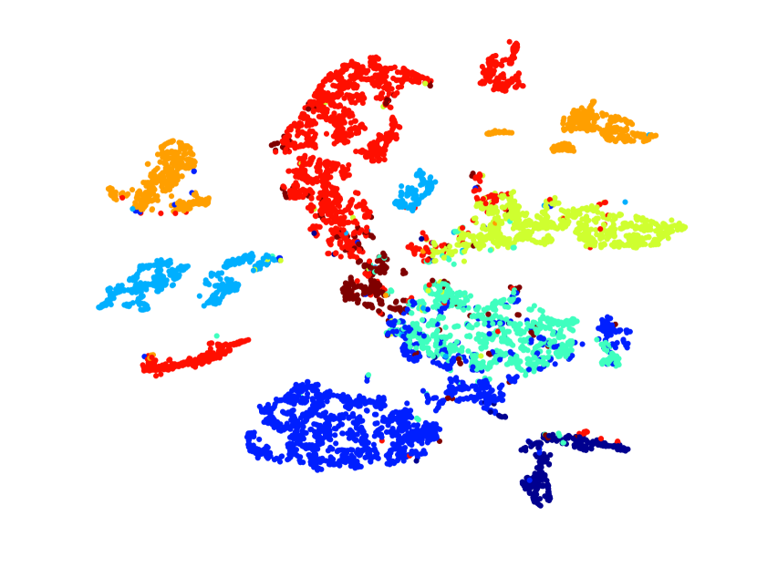
(a) GCN

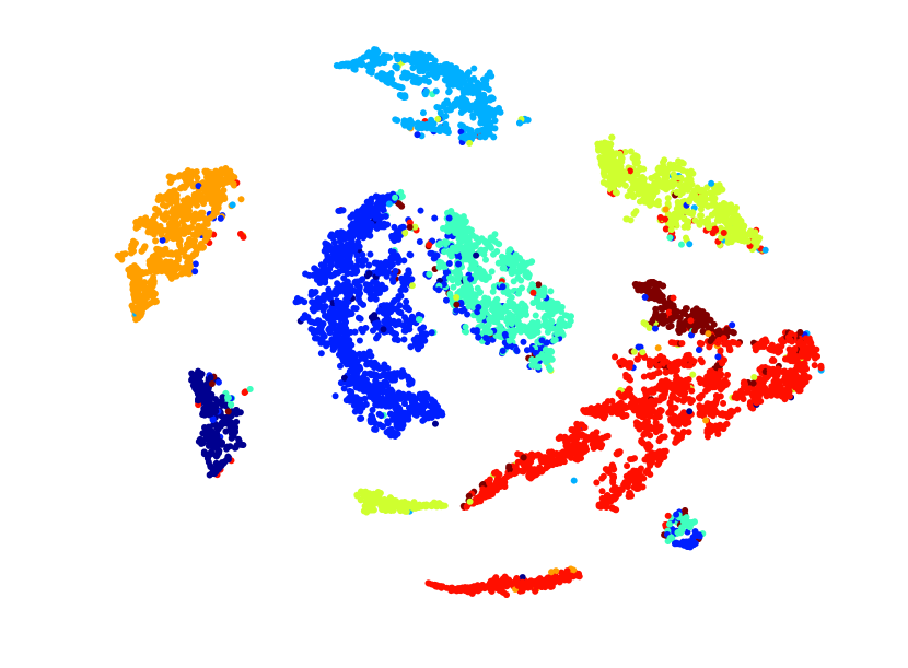
(b) GCN-$\mathrm{AGG}_{\ell_{p}}$

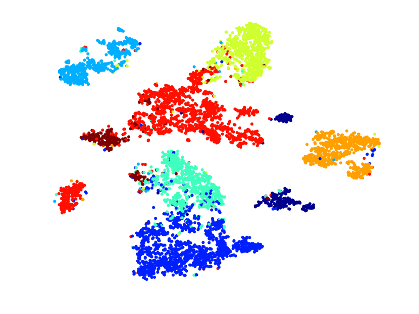
(c) GCN-$\mathrm{AGG}_{\mathcal{P}}$

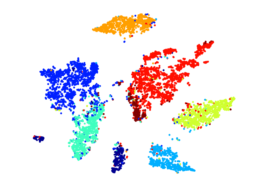
(d) GCN-$\mathrm{AGG}_{\mathcal{S}}$

Figure 1. 2D demonstrations of embedding output by GCN (Kipf and Welling, 2017) and GCN based on nonlinear aggregations on Photo dataset.

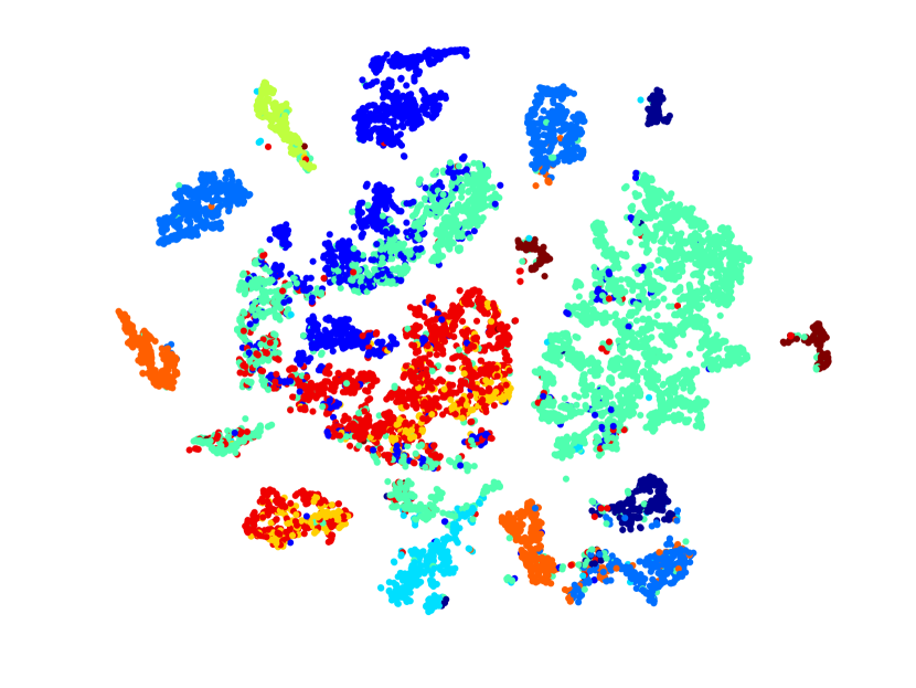
(a) GCN

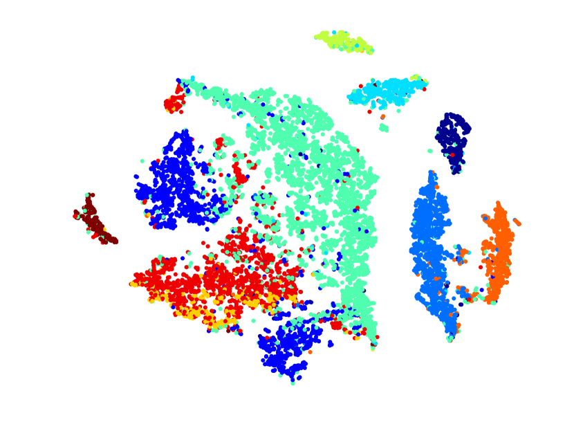
(b) GCN-$\mathrm{AGG}_{\ell_{p}}$

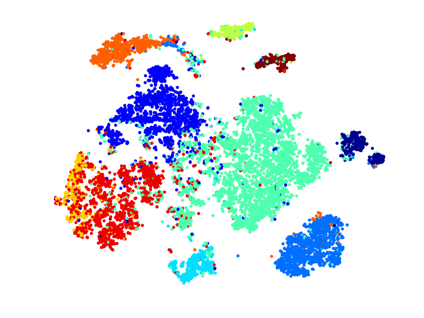
(c) GCN-$\mathrm{AGG}_{\mathcal{P}}$

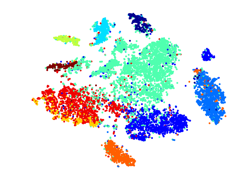
(d) GCN-$\mathrm{AGG}_{\mathcal{S}}$

Figure 2. 2D demonstrations of embedding output by GAT (Veličković et al., 2018) and GAT based on nonlinear aggregations on Computers dataset.

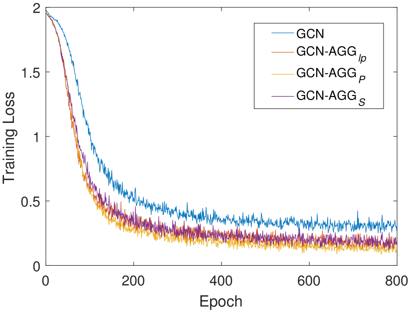
(a) Cora

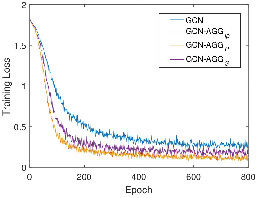
(b) Citeseer

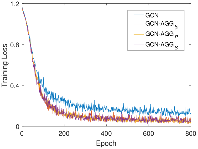
(c) Pubmed

Figure 3. Comparison results of convergence of GCN (Kipf and Welling, 2017) and GCN based on nonlinear aggregations on citation dataset.

4.3. Intuitive Demonstration

Here, we show some visual demonstrations to intuitively demonstrate the effect of the proposed nonlinear aggregations. We first use 2D t-SNE visualization (Maaten and Hinton, 2008) to show some demonstrations. Figure 1 and 2 respectively show the comparison results of GCN (Kipf and Welling, 2017) and GCN-based variants on Amazon Photo and Computers datasets. As shown in Figure 1 and 2, the node embeddings obtained by our proposed nonlinear GCNs are distributed more compactly and clearly than the vanilla GCN (Kipf and Welling, 2017). It is consistent with the experiment results shown in Table $2$ and $3$ which demonstrates the more expressive capacity of the proposed nonlinear aggregators. We then show the convergence property of the nonlinear aggregations based on GNNs. Figure 3 shows the comparison training loss across different epochs of GCN (Kipf and Welling, 2017), GCN-$\mathrm{AGG}_{\ell_{p}}$, GCN-$\mathrm{AGG}_{\mathcal{P}}$ and GCN-$\mathrm{AGG}_{\mathcal{S}}$ on citation datasets . One can note that our proposed three nonlinear GCNs have lower training loss which indicates the higher capacity of the proposed aggregators.

5. Conclusion

In this paper, we re-think the neighborhood aggregation mechanism of GNNs and propose nonlinear message aggregation schemes to extend GNNs’ learning capacity. The proposed nonlinear aggregation operators are general and flexible strategies GNNs which provide the intermediates between the commonly used max and mean/sum aggregations. We integrate our proposed nonlinear aggregators into several GNNs. Experiments on several benchmark datasets show the effectiveness of our proposed nonlinear aggregations on enhancing the learning capacity and performances of GNNs.

References

- (1)
- Cai et al. (2021) Shaofei Cai, Liang Li, Jincan Deng, Beichen Zhang, Zheng-Jun Zha, Li Su, and Qingming Huang. 2021. Rethinking graph neural architecture search from message-passing. In Proceedings of the IEEE/CVF Conference on Computer Vision and Pattern Recognition. 6657–6666.
- Corso et al. (2020) Gabriele Corso, Luca Cavalleri, Dominique Beaini, Pietro Lio, and Petar Velickovic. 2020. Principal Neighbourhood Aggregation for Graph Nets. In Neural Information Processing Systems (NeurIPS) 33.
- Dehmamy et al. (2019) Nima Dehmamy, Albert-Laszlo Barabasi, and Rose Yu. 2019. Understanding the Representation Power of Graph Neural Networks in Learning Graph Topology. In Advances in Neural Information Processing Systems.
- Estrach et al. (2014) Joan Bruna Estrach, Arthur Szlam, and Yann LeCun. 2014. Signal recovery from Pooling Representations. In Proceedings of the 31st International Conference on Machine Learning. 307–315.
- Geisler et al. (2020) Simon Geisler, Daniel Zügner, and Stephan Günnemann. 2020. Reliable Graph Neural Networks via Robust Aggregation. In Advances in Neural Information Processing Systems. 13272–13284.
- Gulcehre et al. (2014) Caglar Gulcehre, Kyunghyun Cho, Razvan Pascanu, and Yoshua Bengio. 2014. Learned-Norm Pooling for Deep Feedforward and Recurrent Neural Networks. In Proceedings of the 2014th European Conference on Machine Learning and Knowledge Discovery. 530–546.
- Hamilton et al. (2017) Will Hamilton, Zhitao Ying, and Jure Leskovec. 2017. Inductive representation learning on large graphs. In Neural Information Processing Systems. 1024–1034.
- He et al. (2021) Tiantian He, L Bai, and Yew Soon Ong. 2021. Learning Conjoint Attentions for Graph Neural Nets. In Advances in Neural Information Processing Systems (NeurIPS) 34. Curran Associates, Inc.
- Kingma and Ba (2015) Diederik P Kingma and Jimmy Ba. 2015. Adam: A method for stochastic optimization. In International Conference on Learning Representations.
- Kipf and Welling (2017) Thomas N. Kipf and Max Welling. 2017. Semi-Supervised Classification with Graph Convolutional Networks. In International Conference on Learning Representations.
- Lee et al. (2017) Chen-Yu Lee, Patrick Gallagher, and Zhuowen Tu. 2017. Generalizing Pooling Functions in CNNs: Mixed, Gated, and Tree. IEEE Transactions on Pattern Analysis and Machine Intelligence 40, 4 (2017), 863–875.
- Li et al. (2018) Q. Li, Z. Han, and X.-M. Wu. 2018. Deeper Insights into Graph Convolutional Networks for Semi-Supervised Learning. In The Thirty-Second AAAI Conference on Artificial Intelligence.
- Maaten and Hinton (2008) Laurens van der Maaten and Geoffrey Hinton. 2008. Visualizing data using t-SNE. Journal of machine learning research 9, Nov (2008), 2579–2605.
- Qian (1999) Ning Qian. 1999. On the momentum term in gradient descent learning algorithms. Neural networks 12, 1 (1999), 145–151.
- Sen et al. (2008) Prithviraj Sen, Galileo Namata, Mustafa Bilgic, Lise Getoor, Brian Galligher, and Tina Eliassi-Rad. 2008. Collective classification in network data. AI magazine 29, 3 (2008), 93–93.
- Shchur et al. (2018) Oleksandr Shchur, Maximilian Mumme, Aleksandar Bojchevski, and Stephan Günnemann. 2018. Pitfalls of graph neural network evaluation. arXiv preprint arXiv:1811.05868 (2018).
- Veličković et al. (2018) Petar Veličković, Guillem Cucurull, Arantxa Casanova, Adriana Romero, Pietro Liò, and Yoshua Bengio. 2018. Graph Attention Networks. International Conference on Learning Representations (2018).
- Wei et al. (2019) Zhen Wei, Jingyi Zhang, Li Liu, Fan Zhu, Fumin Shen, Yi Zhou, Si Liu, Yao Sun, and Ling Shao. 2019. Building detail-sensitive semantic segmentation networks with polynomial pooling. In Proceedings of the IEEE/CVF Conference on Computer Vision and Pattern Recognition. 7115–7123.
- Xu et al. (2019) Keyulu Xu, Weihua Hu, Jure Leskovec, and Stefanie Jegelka. 2019. How Powerful are Graph Neural Networks?. In International Conference on Learning Representations.
- Yang et al. (2019) Liang Yang, Fan Wu, Yingkui Wang, Junhua Gu, and Yuanfang Guo. 2019. Masked Graph Convolutional Network. In International Joint Conference on Artificial Intelligence. 4070–4077.
- Zhao and Akoglu (2020) Lingxiao Zhao and Leman Akoglu. 2020. PairNorm: Tackling Oversmoothing in GNNs. In International Conference on Learning Representations.