Non-Gaussian random matrices determine the stability of Lotka-Volterra communities

Abstract

The eigenvalue spectrum of a random matrix often only depends on the first and second moments of its elements, but not on the specific distribution from which they are drawn. The validity of this universality principle is often assumed without proof in applications. In this letter, we offer a pertinent counterexample in the context of the generalised Lotka-Volterra equations. Using dynamic mean-field theory, we derive the statistics of the interactions between species in an evolved ecological community. We then show that the full statistics of these interactions, beyond those of a Gaussian ensemble, are required to correctly predict the eigenvalue spectrum and therefore stability. Consequently, the universality principle fails in this system. Our findings connect two previously disparate ways of modelling complex ecosystems: Robert May’s random matrix approach and the generalised Lotka-Volterra equations. We show that the eigenvalue spectra of random matrices can be used to deduce the stability of dynamically constructed (or ‘feasible’) communities, but only if the emergent non-Gaussian statistics of the interactions between species are taken into account.

The theory of disordered systems enables one to deduce the behaviour of collections of many interacting constituents, whose interactions are assumed to be random, but fixed in time Mézard et al. (1987). A related discipline, random matrix theory (RMT), is concerned with the eigenvalue spectra of matrices with entries drawn from a joint probability distribution. Both fields have found numerous applications in physics Wigner (1958, 1967) (the study of spin glasses in particular Mézard et al. (1987)), and in other disciplines such as neural networks Aljadeff et al. (2015); Kuczala and Sharpee (2016); Coolen et al. (2005); Rajan and Abbott (2006); Louart et al. (2018), economics Laloux et al. (2000); Bouchaud and Potters (2008) and theoretical ecology May (1972); Allesina and Tang (2012); Opper and Diederich (1992); Galla (2018); Biroli et al. (2018); Altieri et al. (2021).

It is frequently assumed that the distribution of the randomness in RMT or disordered systems is Gaussian, possibly with correlations between different interaction coefficients or matrix entries. Reasons cited for this assumption include analytical convenience, maximum-entropy arguments and the observation that higher-order moments often do not contribute to the results of calculations Edwards and Anderson (1975); Mézard et al. (1987); Galla and Farmer (2013).

In random matrix theory, this latter observation is referred to as the principle of universality Tao and Vu (2010); Tao et al. (2010); Allesina and Tang (2015). The principle states that results obtained for the spectra of Gaussian random matrices frequently also apply to matrix ensembles with non-Gaussian distributions. The conditions for universality to apply are usually mild (higher-order moments of the distribution must fall off sufficiently quickly with the matrix size Tao and Vu (2010); Tao et al. (2010)), and it is often tacitly assumed that these conditions will hold.

In this letter, we offer a pertinent counterexample to the universality principle in RMT. We focus on the ecological community resulting from the dynamics of the generalised Lotka-Volterra equations with random interaction coefficients. The stability of this community is governed by the interactions between species that survive in the long run Stone (2018). This is a sub-matrix of the original interactions, which we will refer to as the ‘reduced interaction matrix’.

Firstly, using dynamic mean-field theory De Dominicis (1978), we obtain the statistics of the elements in the reduced interaction matrix. These turn out to be non-Gaussian (even when the original interaction matrix is Gaussian) and quite intricate. Secondly, we analytically calculate the leading eigenvalue of this non-Gaussian ensemble of random matrices. We show that this eigenvalue is different from the one that we would obtain from a Gaussian ensemble with the same first and second moments as in the reduced interaction matrix. This demonstrates that the principle of universality fails, and indicates that the Gaussian assumption should not be made lightly.

Our results thus connect two previously separate modelling approaches in theoretical ecology: Robert May’s random matrix approach May (1972); Allesina and Tang (2012) and the dynamic generalised Lotka-Volterra equations. We derive the statistics of the emergent random matrix ensemble that reflects the interactions between species in a feasible equilibrium Grilli et al. (2017); Goh and Jennings (1977) (that is, an equilibrium arrived at dynamically). From this ensemble, we then recover the stability criteria derived from the dynamic Lotka-Volterra model.

We start from the generalised Lotka-Volterra equations (GLVEs) Galla (2018); Bunin (2017)

$$\dot{x}_{i}=x_{i}\left[1-x_{i}+\sum_{ij}a_{ij}x_{j}+h_{i}(t)\right],$$ (1)

where the $x_{i}\geq 0$ describe the abundances of species $i=1,\dots,N$. The interaction matrix elements $a_{ij}$ are quenched random variables. We refer to these as the ‘original interaction matrix’ elements. We assume that the mean of each matrix element is $\overline{a_{ij}}=\mu/N$ (we use an overbar to denote averages over the ensemble of interaction matrices), and that they have variance $\mathrm{Var}(a_{ij})=\sigma^{2}/N$. We also allow for correlations between diagonally opposed matrix elements, $\mathrm{Corr}(a_{ij},a_{ji})=\Gamma$, ($-1\leq\Gamma\leq 1$) where $\mathrm{Corr}(a,b)=(\overline{ab}-\overline{a}\overline{b})/\sqrt{\mathrm{Var}(a)\mathrm{Var}(b)}$.

The scaling with $N$ of these moments follows the standard conventions in disordered systems Mézard et al. (1987) and guarantees a well-defined thermodynamic limit $N\to\infty$. All our results are independent of the higher moments of $a_{ij}$ as long as these moments scale sufficiently quickly with $N^{-1}$ [see Refs. Baron et al. (2021); Mézard et al. (1987) and Sec. S1 of the Supplemental Material (SM)]. The external fields $h_{i}(t)$ in Eq. (1) are included for the purposes of analysis, but are ultimately set to zero at the end of calculations and in simulations.

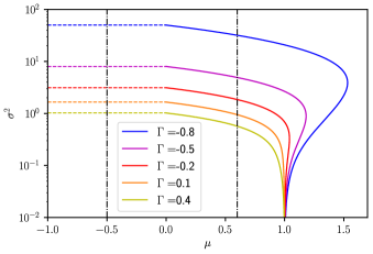
Figure 1: Stability diagram Galla (2018); Bunin (2017) of the GLVE system in the plane spanned by $\mu$ and $\sigma^{2}$ for fixed values of the correlation parameter $\Gamma$. Solid lines indicate the $M\to\infty$ transition, dashed horizontal lines the linear instability. These lines were produced using Eqs. (S20) and (S26) in the SM respectively. Vertical lines mark the values of $\mu$ used in the two panels of Fig. 3. The system has a unique stable fixed point below the dashed lines and to the left of the solid lines.

Previous analyses of this system Galla (2018); Bunin (2017) in the thermodynamic limit have shown that there is a range of parameter combinations $\mu,\sigma^{2}$ and $\Gamma$ for which the dynamics reaches the a unique stable fixed point, independently of the starting conditions. This is the case in the region to the left and below the instability lines in the phase diagram in Fig. 1.

When a fixed point solution is reached, not all species survive, i.e. there are some species for which $x_{i}^{\star}>0$ and others with $x_{i}^{\star}=0$ (we use an asterisk to denote the fixed point). We define $\theta_{i}(t)=\Theta[x_{i}(t)]$, where $\Theta(\cdot)$ is the Heaviside function, to keep track of the surviving species. Using dynamic mean-field theory (DMFT) one can deduce the statistics of the species abundances at the fixed point. Specifically the following can be found analytically (see Galla (2018); Bunin (2017), and the summary in Sec. S1 of the SM),

$$\phi =\lim_{N\to\infty}\frac{1}{N}\sum_{i}\overline{\theta_{i}^{\star}},$$

$$q =\lim_{N\to\infty}\frac{1}{N}\sum_{i}\overline{x_{i}^{\star}x_{i}^{\star}},$$

$$M =\lim_{N\to\infty}\frac{1}{N}\sum_{i}\overline{x_{i}^{\star}}.$$ (2)

These quantities describe the fraction of surviving species, and the first and second moments of the abundances at the fixed point, respectively. Further, we can calculate the following integrated response functions, which will be useful later,

$$\chi =\lim_{t\to\infty}\lim_{N\to\infty}\frac{1}{N}\sum_{i}\int_{0}^{t}dt^{\prime}\overline{\frac{\delta x_{i}(t)}{\delta h_{i}(t^{\prime})}},$$

$$\chi_{{}_{T}} =\lim_{t\to\infty}\lim_{N\to\infty}\frac{1}{N}\sum_{i}\int_{0}^{t}dt^{\prime}\overline{\frac{\delta\theta_{i}(t)}{\delta h_{i}(t^{\prime})}},$$

$$\chi_{2} =\lim_{t\to\infty}\lim_{N\to\infty}\frac{1}{N}\sum_{i}\int_{0}^{t}\int_{0}^{t}dt^{\prime}dt^{\prime\prime}\overline{\frac{\delta^{2}\theta_{i}(t)}{\delta h_{i}(t^{\prime})\delta h_{i}(t^{\prime\prime})}}.$$ (3)

From the DMFT analysis, one can also find the combinations of parameters at which the system is no longer able to support unique stable fixed points. There are two types of transition: (1) the average species abundance can diverge [i.e., $M\to\infty$], or (2) the fixed-point solution can become linearly unstable to perturbations. Closed-form expressions for the critical sets of parameters ($\sigma$, $\Gamma$ and $\mu$) at which each of these transitions occur were derived in Galla (2018); Bunin (2017) and are also given in Sec.  S1 C in the SM. A selection of phase lines for different values of the correlation parameter $\Gamma$ are shown in Fig. 1.

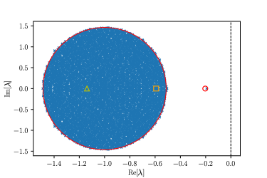
Figure 2: The eigenvalues of the reduced interaction matrix. Results from computer simulations of the GLVE are shown as markers. The solid red curve and the hollow circle show the theoretical predictions for the bulk region and outlier eigenvalue in Eqs. (7) and (11) respectively. Two naive predictions for the outlier that do not take the full statistics of the reduced interaction matrix into account are shown as a yellow triangle ($\lambda_{0}$ in the text) and an orange square ($\lambda_{1}$ in the text). System parameters are $\sigma=1.1$, $\mu=0.9$, $\Gamma=-0.5$, $N=10000$.

We now examine an alternative approach to analysing the stability of the GLVEs in Eq. (1). Namely, we consider the ‘reduced’ interaction matrix (the interaction matrix between only the surviving species). More precisely, this is defined by

$$a^{\prime}_{ij}=a_{ij}-\delta_{ij},$$ (4)

where $i,j\in\mathcal{S}$ (with $\mathcal{S}$ the set of surviving species), and where the shift in the diagonal elements reflects the $-x_{i}$ term inside the square brackets of Eq. (1). It can be shown that a fixed point of the GLVE is stable if and only if all of the eigenvalues of the reduced interaction matrix have negative real parts (see Stone (2018); Biroli et al. (2018), and SM Section S2).

We note that the statistics of the reduced interaction matrix elements are determined by the extinction dynamics in the GLVE system, and are consequently vastly different to those of the original interaction matrix Bunin (2016); Fraboul et al. (2021). For instance, they are non-Gaussian (even when the $a_{ij}$ are Gaussian), and there are correlations between elements sharing only one index (see SM Section S6). This makes the calculation of the eigenvalue spectrum of the reduced interaction matrix a non-trivial task.

As is illustrated in Fig. 2, the spectrum of the reduced interaction matrix consists of a bulk set of eigenvalues and a single outlier. Writing $z_{ij}=a_{ij}-\mu N^{-1}$ (where once again $i,j\in\mathcal{S}$), both the outlier eigenvalue $\lambda_{\mathrm{outlier}}$ and the bulk spectral density $\rho_{\mathrm{bulk}}(\lambda)$ can be obtained from the disorder-averaged resolvent matrix $\underline{\underline{G}}=\overline{\left[\omega\underline{\underline{{\openone}}}-\underline{\underline{z}}\right]^{-1}}$. One has (see Secs. S3 and S5 in the SM and Refs. Sommers et al. (1988); O’Rourke et al. (2014); Benaych-Georges and Nadakuditi (2011); Baron et al. (2021))

$$\rho_{\mathrm{bulk}}(\lambda)=\frac{1}{2\pi N\phi}\mathrm{Re}\left[\frac{\partial\mathrm{Tr}\underline{\underline{G}}}{\partial\omega^{\star}}\right]\bigg{|}_{\omega=1+\lambda},$$ (5)

and

$$\mathcal{G}\left(1+\lambda_{\mathrm{outlier}}\right)=\frac{1}{\mu\phi},$$ (6)

where $\mathcal{G}\left(\omega\right)\equiv(N\phi)^{-1}\overline{\sum_{i,j\in\mathcal{S}}G_{ij}(\omega)}$.

We first briefly discuss the bulk spectrum, for which the results do not run counter to the universality principle. We use a series expansion for a Hermitized version of the resolvent of the reduced interaction matrix (see Sec. S5 of the SM). This standard approach accounts for the non-analytic nature of the resolvent in the bulk region Janik et al. (1997); Feinberg and Zee (1997).

We find that the resulting series for the trace of the resolvent matrix is identical to that of a Gaussian random matrix in the limit $N\to\infty$. That is, we show that the higher-order statistics of the reduced interaction matrix do not contribute to this series and, therefore, that the universality principle holds for the bulk region. The only statistics of the reduced interaction matrix that contribute are $(\sigma^{\prime})^{2}\equiv N_{{}_{\mathcal{S}}}\mathrm{Var}(a_{ij}^{\prime})=\phi\sigma^{2}$ and $\Gamma^{\prime}\equiv\mathrm{Corr}(a_{ij}^{\prime},a_{ji}^{\prime})=\Gamma$ where $N_{{}_{\mathcal{S}}}$ is the number of surviving species (we calculate these statistics in Sec. S6 of the SM). One obtains the familiar elliptic law

$$\rho_{\mathrm{bulk}}(\lambda)=\begin{cases}\frac{1}{\pi(\sigma^{\prime})^{2}[1-(\Gamma^{\prime})^{2}]}\,&\mathrm{if}\,\,\,\frac{(1+x)^{2}}{(1+\Gamma^{\prime})^{2}}+\frac{y^{2}}{(1-\Gamma^{\prime})^{2}}<(\sigma^{\prime})^{2},\\ 0\,&\mathrm{otherwise},\end{cases}$$ (7)

where $\lambda=x+iy$. One can show that the bulk of the eigenvalue spectrum crossing the imaginary axis corresponds to the linear instability of the GLVEs, represented by the dashed horizontal lines in Fig. 1 (see SM Section S5C). This is verified in Fig. 3(a).

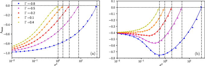
Figure 3: Panel (a): Right edge of the bulk of the eigenvalue spectrum of the reduced interaction matrix versus $\sigma^{2}$ for different values of the system parameter $\Gamma$ and fixed $\mu=-0.5$. Markers are the result of averaging the results of $10$ simulations of the GLVE with $N=4000$. The dashed coloured lines are given by $\lambda_{\mathrm{edge}}=-1+\sigma\sqrt{\phi}(1+\Gamma)$, and the vertical dot-dashed lines are the points where the linear instability occurs in the GLVE (see the dashed lines in Fig. 1). Panel (b): Outlier eigenvalue of the reduced interaction matrix versus $\sigma^{2}$ at fixed $\mu=0.6$ and for the same values of $\Gamma$ as in panel (a). Markers are the result of averaging the results of $10$ simulations with $N=4000$. The solid lines are the analytical result in Eq. (11), and the vertical dot-dashed lines are the points where $M\to\infty$ in the GLVE (see the solid lines in Fig. 1).

We now move on to the outlier eigenvalue, which is a far less trivial matter. We first discuss two candidate expressions for the outlier eigenvalue based upon calculations for Gaussian random matrix ensembles. We show that neither of these expressions are accurate, and that the universality principle fails to predict the outlier eigenvalue. We subsequently derive an accurate expression for the outlier, which also correctly predicts stability.

Noting previous work O’Rourke et al. (2014); Allesina and Tang (2015, 2012); Edwards and Jones (1976), one might perhaps expect that $\mu^{\prime},(\sigma^{\prime})^{2}$ and $\Gamma^{\prime}$ [where $\mu^{\prime}=N_{{}_{\mathcal{S}}}\overline{a_{ij}^{\prime}}$ for $i\neq j$ – see SM Sec. S6A] would be sufficient to predict the outlier eigenvalue of the reduced interaction matrix. Using an established formula for the outlier eigenvalues of Gaussian random matrices Edwards and Jones (1976); O’Rourke et al. (2014), one then obtains $\lambda_{0}=-1+\mu^{\prime}+\Gamma^{\prime}\sigma^{\prime 2}/\mu^{\prime}$.

If we also include the effects of correlations between elements sharing only one index $\gamma^{\prime}=N^{2}\mathrm{Corr}(a^{\prime}_{ij},a^{\prime}_{ki})$ where $k\neq i$), we arrive at (using results from our previous work Baron et al. (2021))

$$\lambda_{1}=-1+\mu^{\prime}+\frac{\mu^{\prime}}{2}\left(1+\frac{\Gamma^{\prime}}{\gamma^{\prime}}\right)\left[\sqrt{1+\frac{4\gamma^{\prime}\sigma^{\prime 2}}{\mu^{\prime}2}}-1\right].$$ (8)

The approach leading to Eq. (8) takes into account all possible correlations for a Gaussian random matrix. We note that correlations between elements in the same row or column also exist in the reduced interaction matrix (see SM Sec. S6A), but these do not affect the location of the outlier Baron et al. (2021).

If the universality principle were to apply to the reduced interaction matrix, then the Gaussian prediction $\lambda_{1}$ and the true outlier eigenvalue would coincide, whether or not the elements of the reduced interaction matrix were also Gaussian distributed. As can be seen in Fig. 4, $\lambda_{1}$ is a better approximation than $\lambda_{0}$, but neither expression correctly predicts the outlier.

We now take into account the full statistics of $a^{\prime}_{ij}$, as we did when calculating the bulk eigenvalue spectrum, and deduce the correct expression for the outlier eigenvalue. In the region of the complex plane outside the bulk (where the outlier resides), the resolvent can be expanded as a series in $1/\omega$

$$\mathcal{G}[\omega] =\frac{1}{\phi N}\overline{\sum_{i,j\in\mathcal{S}}\left[\frac{\delta_{ij}}{\omega}+\frac{z_{ij}}{\omega^{2}}+\sum_{k}\frac{z_{ik}z_{kj}}{\omega^{3}}+\cdots\right]}.$$ (9)

A central step of our calculation is to evaluate each of the averages in the series in Eq. (9) in terms of the fixed-point statistics in Eqs. (2) and (3). This is accomplished via a generating functional approach [see SM Sec. S4A]. For example, we find

$$\frac{1}{N\phi}\overline{\sum_{i,j,k\in\mathcal{S}}z_{ik}z_{kj}}= \phi\Gamma\sigma^{2}+\frac{\sigma^{4}}{\phi}\bigg{[}\chi_{{}_{T}}\chi M+\Gamma\chi_{2}M^{2}$$

$$+\Gamma\chi_{{}_{T}}^{2}q+\Gamma^{2}\chi_{{}_{T}}\chi M\bigg{]}.$$ (10)

Rewriting Eq. (9) in terms of the fixed-point statistics and using diagrammatic techniques to recognise the self-similarity of the resulting series, we arrive at a compact formula for the resolvent [Eq. (S67) in the SM]. Using Eq. (6), we then obtain an implicit set of equations for the outlier eigenvalue

$$\lambda_{\mathrm{outlier}} =-1+\frac{1+\Gamma\phi\sigma^{2}g^{2}}{g}.$$ (11)

Here, the quantity $g$ is given by the unique solution of the following cubic equation that simultaneously satisfies $|g|^{2}<\frac{1}{\phi\sigma^{2}}$,

$$\frac{D(g)}{\mu\phi} =D(g)g+\frac{\sigma^{2}g^{2}}{\phi}\bigg{[}\chi_{{}_{T}}M(1+\Gamma)$$

$$\,\,\,\,\,\,\,\,+\Gamma\sigma^{2}\left(M^{2}\chi_{2}+\chi_{{}_{T}}^{2}q-2\chi\chi_{{}_{T}}M\right)g\bigg{]},$$ (12)

with $D(g)=1-(1+\Gamma)\sigma^{2}\chi g+\Gamma\sigma^{4}\left(\chi^{2}-\chi_{2}q\right)g^{2}$. No approximations have been made in deriving this result, other than assuming the thermodynamic limit. The simulation data in Figs. 3 and 4 verifies that the expression in Eq. (11) accurately predicts the outlier eigenvalue.

One can also demonstrate analytically (see SM Section S4D) that this prediction for the outlier eigenvalue correctly predicts instability of the fixed point of the GLVE system. That is, $\lambda_{\mathrm{outlier}}$ crosses the imaginary axis precisely at locations in parameter space where the $M\to\infty$ transition occurs in the GLVEs. This is also verified in Figs. 3 and 4.

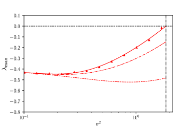
Figure 4: Outlier eigenvalue of the reduced interaction matrix as a function of $\sigma^{2}$, at fixed $\mu=0.6,\Gamma=-0.2$. Markers indicate the results of computer simulations ($N=1000$, averaged over 10 trials). The solid line is from Eq. (11), whereas the dashed line and dot-dashed lines are the two naive predictions $\lambda_{0}$ and $\lambda_{1}$ (respectively) given in the text. The vertical dot-dashed line marks the point at which $M\to\infty$ in the GVLE (see the solid lines in Fig. 1).

To conclude, we have deduced the stability of the generalised Lotka-Volterra system by calculating the eigenvalue spectrum of the interaction matrix of the surviving species. We have shown that results that are derived for Gaussian random matrices, and which are often assumed also to apply to non-Gaussian ensembles, fail in this case. Instead, higher-order statistics of the reduced interaction matrix must be taken into account. We have therefore found a non-contrived class of random matrices for which the universality principle of RMT is not applicable. This demonstrates that there are limitations to results in RMT that are derived making an assumption of Gaussian interactions. Universality should therefore not be invoked without careful consideration.

Our results also have immediate relevance for the field of theoretical ecology. In a widely used approach pioneered by Robert May May (1972, 1971), one supposes that the Jacobian governing small deviations of species abundances about a fixed point can be represented by a random matrix. May does not say what the dynamics are that lead to this Jacobian. One particular objection to this approach is hence that the statistics of May’s random matrices do not necessarily correspond to ‘feasible’ equilibria Stone (2018); Gibbs et al. (2018); Allesina and Tang (2015), i.e. fixed points of a dynamics in which all species abundances are non-negative.

The fixed point of the GLVEs is feasible by construction. Therefore, our work shows that a random matrix approach can be used for studying the stability of a feasible equilibrium in a complex ecosystem. Feasibility is reflected in the higher-order statistics of the interactions between species. Crucially, we find that these intricate statistics cannot be ignored if one is to correctly predict stability.

S1 Dynamic mean-field theory and phase transitions

For completeness, we show in this section how dynamic mean field theory can be used to deduce which sets of interaction statistics of the original Lotka–Volterra community can give rise to stability. This has previously been described in Galla (2018), see in particular the Supplementary Material of this earlier work. In the course of this calculation, we introduce the generating functional formalism and some quantities of interest that will be necessary for quantifying the statistics of the reduced interaction matrix later.

S1.1 Effective process

We begin with the generalised Lotka-Volterra equations Malcai et al. (2002); Brenig (1988)

$$\dot{x}_{i}=x_{i}\left[1-x_{i}+\sum_{j}a_{ij}x_{j}+h_{i}(t)\right],$$ (S1)

where $h_{i}(t)$ is an external field, which is included for the purposes of the calculation, but which is later set to zero. The original interaction matrix elements have the following statistics

$$\overline{a_{ij}} =\mu/N,$$

$$\overline{(a_{ij}-\mu/N)^{2}} =\sigma^{2}/N,$$

$$\overline{(a_{ij}-\mu/N)(a_{ji}-\mu/N)} =\Gamma\sigma^{2}/N.$$ (S2)

The corresponding generating functional De Dominicis (1978), from which the complete statistics of the process can be derived, is

$$Z_{0}[{\mbox{\boldmath$\psi$}}]= \int D[\mathbf{x},\mathbf{\hat{x}}]\exp\left(i\sum_{i}\int dt\left[\hat{x}_{i}(t)\left(\frac{\dot{x}_{i}(t)}{x_{i}(t)}-\left[1-x_{i}(t)+\sum_{j}a_{ij}x_{j}(t)+h_{i}(t)\right]\right)\right]\right)$$

$$\times\exp\left(i\sum_{i}\int dtx_{i}(t)\psi_{i}(t)\right).$$ (S3)

For later convenience, we define $\theta_{i}(t)=\Theta(x_{i})$, where $\Theta(\cdot)$ is the Heaviside function. We also write $\theta_{i}=\lim_{t\to\infty}\theta_{i}(t)$ (in the phase where the system reaches a fixed point). Further, we introduce $\phi(t)$ as the fraction of species that are survive until time $t$ and $N_{{}_{\mathcal{S}}}$ the eventual number of surviving species respectively,

$$\phi(t) =\frac{1}{N}\sum_{i}\theta_{i}(t),$$

$$N_{{{}_{\mathcal{S}}}} =\lim_{t\to\infty}\sum_{i}\theta_{i}(t).$$ (S4)

We write $\phi=N_{\cal S}/N$ for the asymptotic fraction of surviving species in the fixed point phase.

Now, following for example Refs. Sompolinsky and Zippelius (1981); Kirkpatrick and Thirumalai (1987); Opper and Diederich (1992) (especially Ref. Galla (2018) in the context of the current problem), we perform a dynamic mean-field analysis. First one finds the disorder-averaged generating functional $\overline{Z_{0}[{\mbox{\boldmath$\psi$}}]}$, keeping only leading order terms in $N^{-1}$ in the exponent. We note that in taking the disorder average, we do not require $a_{ij}$ to be Gaussian random variables. Merely, we require that the higher moments of $a_{ij}$ decay sufficiently quickly with $N^{-1}$ sothat we only need to include up to quartic order terms in $x_{i}$ and $\hat{x}_{i}$ Baron et al. (2021); Mézard et al. (1987).

Then, by defining appropriate ‘order parameters’ and performing a saddle-point approximation, which is valid in the thermodynamic limit $N\to\infty$, we find the following approximate expression for the generating functional

$$\overline{Z_{0}[{\mbox{\boldmath$\psi$}}]}\approx \prod_{i=1}^{N}\Bigg{[}\int D[x_{i},\widehat{x}_{i}]\exp\left(i\int dt~{}\psi_{i}(t)x_{i}(t)\right)$$

$$\times\exp\left(i\int dt~{}\widehat{x}_{i}(t)\left[\frac{\dot{x}_{i}(t)}{x_{i}(t)}-1+x_{i}(t)-\mu M(t)+\Gamma\sigma^{2}\int dt^{\prime}G(t,t^{\prime})x(t^{\prime})-h_{i}(t)\right]\right)$$

$$\times\exp\left(-\frac{\sigma^{2}}{2}\int dt~{}dt^{\prime}C(t,t^{\prime})\widehat{x}_{i}(t)\widehat{x}_{i}(t^{\prime})\right)\Bigg{]},$$ (S5)

where we note that each species is now statistically equivalent. The quantities $M(t)$, $G(t,t^{\prime})$ and $C(t,t^{\prime})$ are defined self-consistently via

$$M(t) \equiv\langle x_{i}(t)\rangle,$$

$$R(t,t^{\prime}) \equiv\left\langle\frac{\delta x_{i}(t)}{\delta h_{i}(t^{\prime})}\right\rangle=-i\left\langle x_{i}(t)\hat{x}_{i}(t^{\prime})\right\rangle,$$

$$C(t,t^{\prime}) \equiv\langle\eta_{i}(t)\eta_{i}(t^{\prime})\rangle=\langle x_{i}(t)x_{i}(t^{\prime})\rangle,$$ (S6)

where the angular brackets represent averages with respect to the disorder-averaged generating functional

$$\langle\cdots\rangle= \int D[\mathbf{x},\mathbf{\hat{x}}]\left[\cdots\right]\overline{\exp\left(i\sum_{i}\int dt\left[\hat{x}_{i}(t)\left(\frac{\dot{x}_{i}(t)}{x_{i}(t)}-\left[1-x_{i}(t)+\sum_{j}a_{ij}x_{j}(t)\right]\right)\right]\right)}$$

$$\approx \frac{1}{\Omega}\int D[\mathbf{x},\mathbf{\hat{x}}]\left[\cdots\right]\exp\left(-\frac{\sigma^{2}}{2}\int dt~{}dt^{\prime}\sum_{i}C(t,t^{\prime})\widehat{x}_{i}(t)\widehat{x}_{i}(t^{\prime})\right)$$

$$\times\exp\left(i\int dt~{}\sum_{i}\widehat{x}_{i}(t)\left[\frac{\dot{x}_{i}(t)}{x_{i}(t)}-1+x_{i}(t)-\mu M(t)+\Gamma\sigma^{2}\int dt^{\prime}G(t,t^{\prime})x(t^{\prime})\right]\right),$$ (S7)

where $\Omega$ is a normalisation constant. We also find that for large $N$

$$\phi(t) =\langle\theta_{i}(t)\rangle,$$

$$N_{{}_{\mathcal{S}}} =N\lim_{t\to\infty}\phi(t).$$ (S8)

We thus see that in the thermodynamic limit, the disorder-averaged generating functional can be written as the product of $N$ identical generating functionals. From the form of these factors one can deduce that each species can be approximated as obeying a self-consistent stochastic process of the form

$$\dot{x}_{i} =x_{i}\left[1-x_{i}+\mu M(t)+\Gamma\sigma^{2}\int dt^{\prime}R(t,t^{\prime})x_{i}(t^{\prime})+\sigma\eta_{i}(t)\right],\quad\langle\eta_{i}(t)\eta_{i}(t^{\prime})\rangle=C(t,t^{\prime}),$$ (S9)

where we use the fact that the angular brackets can also be thought of as averages over realisations of the coloured noise $\eta_{i}(t)$. Similar effective single-species dynamics have also been obtained using the cavity approach Roy et al. (2019). We note that the response function $R(t,t^{\prime})$ and the average abundance $M(t)$ are also to be obtained self-consistently as averages over realisations of the process in Eq. (S9). We note further that the site index $i$ serves no further purpose in Eq. (S9), we will therefore drop this index from now on.

For the sake of later analysis, we also define the following response functions

$$T(t,t^{\prime}) \equiv\left\langle\frac{\delta\theta(t)}{\delta h(t^{\prime})}\right\rangle=-i\langle\theta_{i}(t)\hat{x}_{i}(t^{\prime})\rangle,$$

$$T_{2}(t,t^{\prime}) \equiv\left\langle\frac{\delta^{2}\theta(t)}{\delta h(t^{\prime})\delta h(t^{\prime\prime})}\right\rangle=-\langle\theta(t)\hat{x}(t^{\prime})\hat{x}(t^{\prime\prime})\rangle.$$ (S10)

S1.2 Fixed-point analysis

We now wish to construct the stability plot in Fig. 1 in the main text, following Galla (2018). First, we note that the fixed point quantities defined in Eqs. (2) and (3) of the main text can also be written in terms of averages over realisations of the effective dynamics

$$\chi =\lim_{t\to\infty}\int_{0}^{t}dt^{\prime}\left\langle\frac{1}{\sigma}\frac{\delta x(t)}{\delta\eta(t^{\prime})}\right\rangle,$$

$$\chi_{{}_{T}} =\lim_{t\to\infty}\int_{0}^{t}dt^{\prime}\left\langle\frac{1}{\sigma}\frac{\delta\theta(t)}{\delta\eta(t^{\prime})}\right\rangle,$$

$$\chi_{2} =\lim_{t\to\infty}\int_{0}^{t}\int_{0}^{t}dt^{\prime}dt^{\prime\prime}\left\langle\frac{1}{\sigma^{2}}\frac{\delta^{2}\theta(t)}{\delta\eta(t^{\prime})\delta\eta(t^{\prime\prime})}\right\rangle,$$

$$\phi =\lim_{t\to\infty}\langle\theta(t)\rangle,$$

$$q =\lim_{t\to\infty}\langle x(t)x(t^{\prime})\rangle,$$

$$M =\lim_{t\to\infty}\langle x(t)\rangle.$$ (S11)

Setting $\dot{x}=0$ in Eq. (S9) after dropping the index $i$, we thus obtain the following expression for the fixed points of the surviving species

$$x^{\star}=\frac{1+\mu M+\sigma\sqrt{q}z}{1-\Gamma\sigma^{2}\chi}\Theta\left(\frac{1+\mu M+\sigma\sqrt{q}z}{1-\Gamma\sigma^{2}\chi}\right),$$ (S12)

where $z$ is a Gaussian random variable with zero mean and unit variance. Following Galla (2018), this then leads to the self-consistency relations (with $Dz=\frac{dz}{\sqrt{2\pi}}e^{-z^{2}/2}$)

$$\chi = \frac{1}{1-\Gamma\sigma^{2}\chi}\int_{-\infty}^{\Delta}Dz,$$

$$M = \frac{\sqrt{q}\sigma}{1-\Gamma\sigma^{2}\chi}\int_{-\infty}^{\Delta}Dz~{}(\Delta-z),$$

$$1 = \frac{\sigma^{2}}{(1-\Gamma\sigma^{2}\chi)^{2}}\int_{-\infty}^{\Delta}Dz~{}(\Delta-z)^{2},$$ (S13)

where $\Delta=\frac{1+\mu M}{\sqrt{q}\sigma}$. We also have

$$\phi =\int_{-\infty}^{\Delta}Dz,$$

$$\chi_{{}_{T}} =\frac{d\phi}{dh}=\frac{1}{\sigma\sqrt{2\pi q}}e^{-\Delta^{2}/2},$$

$$\chi_{2} =\frac{d^{2}\phi}{dh^{2}}=-\frac{\Delta}{\sigma^{2}q\sqrt{2\pi}}e^{-\Delta^{2}/2}.$$ (S14)

For positive integers $\ell$ we now define the following truncated Gaussian integrals

$$w_{\ell}(\Delta)\equiv\int_{-\infty}^{\Delta}Dz~{}(\Delta-z)^{\ell}.$$ (S15)

Explicitly, we have

$$w_{0}(\Delta) = \frac{1}{2}\left[1+{\rm erf}\left(\frac{\Delta}{\sqrt{2}}\right)\right],$$

$$w_{1}(\Delta) = \frac{1}{2}\left[e^{-\Delta^{2}/2}\sqrt{\frac{2}{\pi}}+\Delta\left(1+{\rm erf}\left(\frac{\Delta}{\sqrt{2}}\right)\right)\right],$$

$$w_{2}(\Delta) = \frac{1}{2}\left(1+\Delta^{2}\right)\left[1+{\rm erf}\left(\frac{\Delta}{\sqrt{2}}\right)\right]+\frac{1}{\sqrt{2\pi}}e^{-\Delta^{2}/2}\Delta.$$ (S16)

One also has the relation

$$w_{2}(\Delta)=w_{0}(\Delta)+\Delta w_{1}(\Delta).$$ (S17)

After some algebra, we derive from Eqs. (S13) a single equation that we can solve to find $\Delta$ for a given $(\mu,\sigma,\Gamma)$ [the interaction statistics of the original community – see Eq. (S2)]. That is, we solve the following numerically for $\Delta$

$$\sigma^{2} =\frac{w_{2}(\Delta)}{[w_{2}(\Delta)+\Gamma w_{0}(\Delta)]^{2}}.$$ (S18)

We see therefore that $\Delta$ is independent of $\mu$. We can then obtain the remaining fixed-point order parameters by substituting this value of $\Delta$ into

$$\chi = w_{0}+\Gamma\frac{w_{0}^{2}}{w_{2}},$$

$$\frac{1}{M} = \frac{\Delta}{w_{1}}\frac{w_{2}}{w_{2}+\Gamma w_{0}}-\mu,$$

$$q = \left(\frac{M}{\sigma w_{1}}\frac{w_{2}}{w_{2}+\Gamma w_{0}}\right)^{2},$$

$$\phi = w_{0},$$

$$\chi_{{}_{T}} = \frac{1}{\sigma\sqrt{q}}(w_{1}-\Delta w_{0}),$$

$$\chi_{2} = -\frac{\Delta}{\sigma^{2}q}(w_{1}-\Delta w_{0}).$$ (S19)

S1.3 Transitions

The validity of the fixed point solution can break down in two different ways, indicating the onset of instability.

S1.3.1 Diverging abundances

One transition occurs when the average fixed-point abundance diverges, i.e. $M\to\infty$. Consulting Eqs. (S18) and (S19), the sets of points at which this transition occurs (for a fixed $\Gamma$) obey

$$\mu =\frac{\Delta}{w_{1}}\frac{w_{2}}{w_{2}+\Gamma w_{0}},$$

$$\sigma^{2} =\frac{w_{2}}{(w_{2}+\Gamma w_{0})^{2}}.$$ (S20)

These can be viewed as a parametric set of equations in $\Delta$ for the phase transition line in the $\mu$–$\sigma$ plane (with $\Gamma$ held fixed). From these equations, the solid lines in Fig. 1 in the main text can be produced.

S1.3.2 Linear instability

The other transition occurs when the fixed point becomes linearly unstable to perturbations. Linearising the effective process in Eq. (S9) about its fixed point, we obtain for small perturbations $\epsilon(t)=x(t)-x^{\star}$ and $\delta\eta(t)=\eta(t)-\sigma\sqrt{q}z$ that arise from an external white noise $\xi(t)$

$$\dot{\epsilon} =x^{\star}\left[-\epsilon+\Gamma\sigma^{2}\int dt^{\prime}G(t,t^{\prime})\epsilon(t^{\prime})+\sigma\delta\eta(t)+\xi\right],$$ (S21)

where $x^{\star}$ satisfies Eq. (S12) and $\langle\xi(t)\xi(t^{\prime})\rangle=\delta(t-t^{\prime})$ and $\langle\xi\rangle=0$. Taking the Fourier transform (indicated by a tilde in the following), rearranging and taking the limit $\omega\to 0$ Opper and Diederich (1992), we find

$$\lim_{\omega\to 0}\langle|\tilde{\epsilon}(\omega)|^{2}\rangle =\frac{1}{(1-\Gamma\sigma^{2}\chi)^{2}/\phi-\sigma^{2}}.$$ (S22)

The object on the right diverges when

$$(1-\Gamma\sigma^{2}\chi)^{2}= \phi\sigma^{2},$$ (S23)

indicating that our solution no longer holds and that the system becomes unstable to perturbations. Using Eqs. (S13) we therefore deduce

$$\phi =\frac{1}{\sigma^{2}(1+\Gamma)^{2}},$$

$$\chi =\frac{1}{\sigma^{2}(1+\Gamma)}.$$ (S24)

Finally, using Eqs. (S19), we see that

$$\chi\sigma^{2} =\frac{\phi}{w_{2}+\Gamma\phi}=\frac{1}{1+\Gamma},$$

$$\Rightarrow w_{2} =\phi,$$

$$\Rightarrow\phi =1/2$$

$$\Rightarrow\Delta =0.$$ (S25)

So finally, substituting $\phi=1/2$ into the first of Eqs. (S24), we see that an instability occurs when

$$\sigma^{2}=\frac{2}{(1+\Gamma)^{2}},$$ (S26)

as previously derived in Galla (2018). Using Eq. (S26), one obtains the dashed horizontal lines in Fig. 1 in the main text.

S2 Reduced interaction matrix and Jacobian matrix

S2.1 Reduced Jacobian and reduced interaction matrix

We now introduce and discuss several different matrices. One is the full (or original) $N\times N$ interaction matrix $\underline{\underline{a}}$, with elements $a_{ij}$. A second matrix is what we call the ‘reduced interaction matrix’, $\underline{\underline{a}}^{\prime}$. This is obtained from the original interaction matrix by removing all rows and columns corresponding to extinct species, and by carrying out a shift of the diagonal elements by $-1$ to capture the $-x_{i}$ term inside the square bracket of the generalised Lotka-Volterra Eqs. (1) in the main paper. This reduced matrix is of size $N_{S}\times N_{S}$, where $N_{S}$ is the number of surviving species in the long run [see Eq. (S4)]. We denote the reduced interaction matrix elements by $a^{\prime}_{ij}=(a_{ij}-\delta_{ij})$ for $i,j\in\mathcal{S}$, where $\mathcal{S}$ is the set of surviving species as $t\to\infty$.

Similarly, we also define the full and reduced Jacobian matrices of the GLVE, $\underline{\underline{J}}$ and $\underline{\underline{J}}^{\prime}$ respectively. The (full) Jacobian of the system (about the fixed point $\underline{x}^{\star}$) takes the form

$$J_{ij}=\delta_{ij}\left[1-x^{\star}_{i}+\sum_{j}a_{ij}x^{\star}_{j}\right]+x_{i}^{\star}\left(a_{ij}-\delta_{ij}\right),$$ (S27)

where $i,j=1,\dots,N$.

We now imagine that (in a particular realisation) we re-arrange the species indices such that $i=1,\dots,N_{S}$ are the surviving species, and $i=N_{S}+1,\dots,N$ the extinct species. This can always be done retrospectively without loss of generality. The Jacobian can then be written in block form

$$\underline{\underline{J}}=\left(\begin{array}[]{cc}\underline{\underline{J}}^{\prime}&\underline{\underline{B}}\\ \underline{\underline{0}}&\underline{\underline{D}}\end{array}\right),$$ (S28)

The reduced Jacobian $\underline{\underline{J}}^{\prime}$ makes up the upper left $N_{S}\times N_{S}$ block. We label the lower right-hand $(N-N_{{}_{\mathcal{S}}})\times(N-N_{{}_{\mathcal{S}}})$ block $\underline{\underline{D}}$. The upper-right block is labelled $\underline{\underline{B}}$. For an extinct species $i$ we have $J_{ij}=0$ for all $j\neq i$ [Eq. (S27)]. Hence the block on the lower left is zero, and the matrix $\underline{\underline{D}}$ is diagonal.

We hence have

$$\mathrm{det}\left(\underline{\underline{J}}-\lambda{\openone}_{N}\right)=\mathrm{det}(\underline{\underline{J}}^{\prime}-\lambda{\openone}_{N_{S}})\mathrm{det}(\underline{\underline{D}}-\lambda{\openone}_{N-N_{S}}),$$ (S29)

(where ${\openone}_{N}$ is the identity matrix of size $N\times N$), and the eigenvalues of $\underline{\underline{J}}$ are given by the combined eigenvalues of $\underline{\underline{J}}^{\prime}$ and $\underline{\underline{D}}$.

We focus first on a species $i$ that goes extinct ($x_{i}^{*}=0$). For such a species, one finds $J_{ii}=1-x_{i}^{*}+\sum_{j}a_{ij}x^{\star}_{j}<0$. Hence $\underline{\underline{D}}$ is a diagonal matrix with only negative diagonal entries, and so we need only consider the eigenvalues of $\underline{\underline{J^{\prime}}}$ to determine stability.

Now we consider the reduced Jacobian $\underline{\underline{J}}^{\prime}$. Given that $1-x^{\star}_{i}+\sum_{j}a_{ij}x^{\star}_{j}=0$ for values of $i$ corresponding to surviving species, we see from Eq. (S27) that the reduced Jacobian matrix of the Lotka-Volterra system takes the simple form

$$J_{ij}^{\prime}=x_{i}^{\star}a_{ij}^{\prime},$$ (S30)

where $i,j\in{\cal S}$. Examples of eigenvalue spectra of the reduced Jacobian and the reduced interaction matrix are given in Fig. S1.

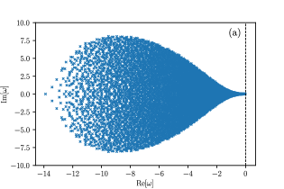
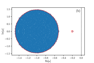
Figure S1: Panel (a): Example eigenvalue spectrum of the reduced Jacobian. Panel (b): Example spectrum of the reduced interaction matrix. The red line and circle in panel (b) show the analytical predictions for the bulk region and outlier eigenvalue in Eqs. (S95) and (S68) respectively. Parameters are $\sigma=1.1$, $\mu=0.9$, $\Gamma=-0.5$, $N=4000$.

S2.2 Reduced Jacobian is not practical for determining stability

One notes that the eigenvalue spectrum of the reduced Jacobian comes arbitrarily close to the imaginary axis. This is observed for all values of the model parameters in the phase with a unique fixed point. This is due to the fact that the distribution of fixed-point abundances $x_{i}^{\star}$ of the surviving species comes arbitrarily close to zero. (The distribution of abundances of surviving species is a Gaussian clipped at zero, see e.g. Galla (2018).) For this reason, it is not helpful to study the spectrum of the full or reduced Jacobian when determining stability – one cannot identify points in parameter space at which one eigenvalue first touches the imaginary axis, or crosses into the right half of the complex plane.

S2.3 Spectrum of reduced interaction matrix determines stability

We now argue as to why we need only consider the eigenvalue spectrum of the reduced interaction matrix $\underline{\underline{a}}^{\prime}$ when determining stability instead of the reduced Jacobian. We note for the following discussion that the leading eigenvalues of both the reduced Jacobian and the reduced interaction matrix are real.

Eq. (S30) indicates that the reduced Jacobian matrix can be written as the product of the reduced interaction matrix and a diagonal matrix of species abundances. The determinant of $\underline{\underline{J}}^{\prime}$ is therefore the product of the determinants of these two matrices. The abundances in the diagonal matrix are strictly positive, and therefore $\mbox{sgn}(\det\,\underline{\underline{D}})=1$. Hence, $\mbox{sgn}(\det\,\underline{\underline{J}}^{\prime})=\mbox{sgn}(\det\,\underline{\underline{a}}^{\prime})$. If the determinant of the reduced Jacobian changes sign as parameters are varied (indicating loss of stability), so must therefore that of the reduced interaction matrix and vice versa.

Imagine now we start in a region of parameter space for which the fixed point is stable and that we then vary the model parameters. The fixed point becomes unstable at the point where the leading eigenvalue of the reduced interaction matrix becomes positive. Therefore, we can deduce the stability of the system by examining the eigenvalue spectrum of the reduced interaction matrix only. A similar argument to this was given in Ref. Stone (2018). Crucially (as we will see), the leading eigenvalue of the reduced interaction matrix is genuinely negative in the stable regime (i.e., not infinitessimally close to the imaginary axis like that of the reduced Jacobian), and only reaches the axis at the point of instability.

S2.4 Components of the spectrum of the reduced interaction matrix

As illustrated in Fig. S1 (b), there is an elliptic ‘bulk’ region of the complex plane, to which the majority of the eigenvalues of the reduced interaction matrix are confined, and a single outlier. We therefore write the eigenvalue density of the reduced interaction matrix in the form

$$\rho(\omega)=\rho_{\mathrm{bulk}}(\omega)+\frac{1}{N_{{}_{\mathcal{S}}}}\delta(\omega-\lambda_{\mathrm{outlier}}).$$ (S31)

In the following sections, we deduce both the bulk eigenvalue density and the location of the outlier eigenvalue. We show that the point in parameter space at which the outlier crosses the imaginary axis is given by Eq. (S20). We also demonstrate that the bulk spectrum crosses into the right half of the complex plane at the point described by Eq. (S26).

S3 Finding the outlier eigenvalue – general approach

The outlier eigenvalue, $\lambda_{\mathrm{outlier}}$, of the reduced interaction matrix by definition must obey

$$\det\left(\lambda_{\mathrm{outlier}}{\openone}_{N_{{}_{\mathcal{S}}}}-\underline{\underline{a}}^{\prime}\right)=0,$$ (S32)

where ${\openone}_{N_{{}_{\mathcal{S}}}}$ is the identity matrix of size $N_{{}_{\mathcal{S}}}\times N_{{}_{\mathcal{S}}}$.

Suppose we introduce a uniform matrix $\underline{\underline{u}}$ with all entries equal to $\nu/N_{{}_{\mathcal{S}}}$. Following Refs. O’Rourke et al. (2014); Benaych-Georges and Nadakuditi (2011) and using Sylvester’s determinant identity, one finds

$$\det\left({\openone}_{N_{{}_{\mathcal{S}}}}-\frac{\nu}{N_{{}_{\mathcal{S}}}}\underline{\underline{G}}\right)=1-\frac{\nu}{N_{{}_{\mathcal{S}}}}\sum_{ij}G_{ij}(1+\lambda_{\mathrm{outlier}})=0,$$ (S33)

where we have introduced the resolvent matrix $\underline{\underline{G}}(1+\lambda_{\mathrm{outlier}})=[\lambda_{\mathrm{outlier}}{\openone}_{N_{{}_{\mathcal{S}}}}-(\underline{\underline{a}}^{\prime}-\underline{\underline{u}})]^{-1}$. Thus, to find the outlier eigenvalue, one has to find the resolvent matrix and solve Eq. (S33) for $\lambda_{\mathrm{outlier}}$. We stress that all elements of the resolvent are required in Eq. (S33), not only the diagonal entries.

We note that we have the freedom to choose the value of $\nu$, as long as it is non-zero and $\lambda_{\mathrm{outlier}}{\openone}_{N_{{}_{\mathcal{S}}}}-(\underline{\underline{a}}^{\prime}-\underline{\underline{u}})$ remains invertible. We exploit this freedom to simplify the calculation of the resolvent in the next section.

S4 Using the generating functional to find the resolvent of the reduced interaction matrix

S4.1 Series expansion for the resolvent of the reduced interaction matrix

To simplify our calculation of the resolvent matrix, we choose $\nu=\phi\mu$ in Eq. (S33). Letting $z_{ij}=\lim_{t\to\infty}[a_{ij}-\mu N^{-1}]\theta_{i}\theta_{j}$ [see the discussion preceding Eq. (S4) for a definition of $\theta_{i}$], we see that the disorder-averaged resolvent matrix that we must evaluate to find the outlier can be expressed as the following series [see Eq. (7) in the main text]

$$\mathcal{G}[\omega] \equiv\overline{N_{{}_{\mathcal{S}}}^{-1}\sum_{i,j\in\mathcal{S}}G_{ij}(\omega)}=\overline{N_{{}_{\mathcal{S}}}^{-1}\sum_{i,j\in\mathcal{S}}\left[\delta_{ij}\omega-z_{ij}\right]^{-1}}$$

$$=\overline{N_{{}_{\mathcal{S}}}^{-1}\sum_{ij}\left[\omega^{-1}\delta_{ij}\theta_{i}\theta_{j}+\omega^{-2}z_{ij}+\omega^{-3}\sum_{k}z_{ik}z_{kj}+\cdots\right]},$$ (S34)

where sums over $i,j\in\mathcal{S}$ denote a sum over the reduced interaction matrix elements, whereas sums over $ij$ indicate a sum over all elements of the original interaction matrix.

To find the terms of this series, we now construct the following generating functional

$$Z[{\mbox{\boldmath$\psi$}},{\mbox{\boldmath$\lambda$}}] =\int D[\mathbf{x},\mathbf{\hat{x}}]\exp\left(i\sum_{i}\int dt\left[\hat{x}_{i}(t)\left(\frac{\dot{x}_{i}(t)}{x_{i}(t)}-\left[1-x_{i}(t)+\sum_{j}a_{ij}x_{j}(t)+h_{i}(t)\right]\right)\right]\right)$$

$$\times\exp\left(-i\int dt\,\sum_{ij}\lambda_{ij}(t)[a_{ij}-\mu N^{-1}]\theta_{i}(t)\theta_{j}(t)\right)\exp\left(i\sum_{i}\int dtx_{i}(t)\psi_{i}(t)\right).$$ (S35)

This generating functional has the same form as in Eq. (S3), with the addition of another source term containing the auxiliary variables $\lambda_{ij}(t)$, which we introduce in this step. The dynamics of $x_{i}(t)$ are still constrained to follow the Lotka-Volterra equations in Eq. (S1), but by functionally differentiating with respect to $\lambda_{ij}(t)$, we can obtain the terms in the series in Eq. (S34). For example,

$$\overline{\frac{\delta Z}{\delta\lambda_{ij}(t)}}\bigg{\rvert}_{{\mbox{\boldmath$\psi$}}=0,\lambda=0}=-i\overline{[a_{ij}-\mu N^{-1}]\theta_{i}(t)\theta_{j}(t)}=-i\overline{z_{ij}}.$$ (S36)

We now find for the disorder-averaged resolvent [from which we can find the outlier eigenvalue via Eq. (S33)]

$$\mathcal{G}[\omega]=\overline{N_{{}_{\mathcal{S}}}^{-1}\sum_{ij}\lim_{t\to\infty}\left[\omega^{-1}\delta_{ij}\theta_{i}\theta_{j}+i\omega^{-2}\frac{\delta Z}{\delta\lambda_{ij}(t)}-\omega^{-3}\sum_{k}\frac{\delta^{2}Z}{\delta\lambda_{ik}(t)\delta\lambda_{kj}(t)}+\cdots\right]}\bigg{\rvert}_{{\mbox{\boldmath$\psi$}}=0,\lambda=0}.$$ (S37)

S4.2 Evaluating the series for the resolvent

Setup and strategy for evaluation of the series

To find the terms of the series in Eq. (S37), we begin by calculating the following average that appears in the expression for $\overline{Z[{\mbox{\boldmath$\psi$}},{\mbox{\boldmath$\lambda$}}]}$

$$A =\overline{\exp\left(i\sum_{i}\int dt\left[-\sum_{j}a_{ij}\hat{x}_{i}(t)x_{j}(t)\right]\right)\exp\left(-i\int dt\,\sum_{ij}\lambda_{ij}(t)[a_{ij}-\mu/N]\theta_{i}(t)\theta_{j}(t)\right)}$$

$$=\exp\left(-i\sum_{i}\int dt\left[\sum_{j}\frac{\mu}{N}\hat{x}_{i}(t)x_{j}(t)\right]\right)$$

$$\times\exp\left(-\frac{\sigma^{2}}{2N}\sum_{ij}\left[\int dt\,\hat{x}_{i}(t)x_{j}(t)+\lambda_{ij}(t)\theta_{i}(t)\theta_{j}(t)\right]^{2}\right)$$

$$\times\exp\left(-\frac{\sigma^{2}}{2N}\sum_{ij}\Gamma\left[\int dt\,\hat{x}_{i}(t)x_{j}(t)+\lambda_{ij}(t)\theta_{i}(t)\theta_{j}(t)\right]\left[\int dt\,\hat{x}_{j}(t)x_{i}(t)+\lambda_{ji}(t)\theta_{i}(t)\theta_{j}(t)\right]\right).$$ (S38)

One thus finds that the derivatives in Eq. (S37) can be written as, for example,

$$\overline{\frac{\delta^{2}Z}{\delta\lambda_{ik}\delta\lambda_{kj}}}\bigg{|}_{\psi=0,\lambda=0}=\left\langle\frac{1}{A}\frac{\delta^{2}A}{\delta\lambda_{ik}\delta\lambda_{kj}}\right\rangle\bigg{|}_{\lambda=0},$$ (S39)

where we note that there are two kinds of averages here: an average over realisations of the interaction coefficients represented by $\overline{\cdots}$ and an average over the dynamics enforced by the disorder averaged generating functional denoted by angular brackets $\langle\cdots\rangle$ [see Eq. (S7)].

The series in Eq. (S37) can therefore be rewritten

$$\mathcal{G}[\omega] =\frac{1}{\phi N}\sum_{ij}\lim_{t\to\infty}\left[\frac{\delta_{ij}\theta_{i}\theta_{j}}{\omega}+\frac{i}{\omega^{2}}\left\langle\frac{1}{A}\frac{\delta A}{\delta\lambda_{ij}(t)}\right\rangle-\frac{1}{\omega^{3}}\sum_{k}\left\langle\frac{1}{A}\frac{\delta^{2}A}{\delta\lambda_{ik}(t)\delta\lambda_{kj}(t)}\right\rangle+\cdots\right]\bigg{|}_{\lambda=0}.$$ (S40)

Let us now begin to construct the series for the resolvent in Eq. (S40). Consider the derivatives of $A$:

$$B_{ij}(t) \equiv\frac{1}{A}\frac{\delta A}{\delta\lambda_{ij}(t)}$$

$$=-\Bigg{[}\theta_{i}(t)\theta_{j}(t)\frac{\sigma^{2}}{N}\int dt^{\prime}\hat{x}_{i}(t^{\prime})x_{j}(t^{\prime})+\theta_{i}(t)\theta_{j}(t)\frac{\sigma^{2}}{N}\int dt^{\prime}\theta_{i}(t^{\prime})\theta_{j}(t^{\prime})\lambda_{ij}(t^{\prime})$$

$$+\theta_{i}(t)\theta_{j}(t)\frac{\Gamma\sigma^{2}}{N}\int dt^{\prime}\hat{x}_{j}(t^{\prime})x_{i}(t^{\prime})+\theta_{i}(t)\theta_{j}(t)\frac{\Gamma\sigma^{2}}{N}\int dt^{\prime}\theta_{i}(t^{\prime})\theta_{j}(t^{\prime})\lambda_{ji}(t^{\prime})\Bigg{]},$$

$$\frac{\delta^{2}A}{\delta\lambda_{ik}(t)\delta\lambda_{kj}(t)} =\left[\frac{\delta B_{ik}(t)}{\delta\lambda_{kj}(t)}+B_{ik}B_{kj}\right]A,$$

$$\frac{\delta^{3}A}{\delta\lambda_{ik}(t)\delta\lambda_{kl}(t)\lambda_{lj}(t)} =\left[B_{ik}\frac{\delta B_{kl}(t)}{\delta\lambda_{lj}(t)}+\frac{\delta B_{ik}(t)}{\delta\lambda_{kl}(t)}B_{lj}+B_{ik}B_{kl}B_{lj}\right]A,$$

$$\frac{\delta^{4}A}{\delta\lambda_{ik}(t)\delta\lambda_{kl}(t)\lambda_{lm}(t)\lambda_{mj}(t)} =\Bigg{[}\frac{\delta B_{ik}(t)}{\delta\lambda_{kl}(t)}\frac{\delta B_{lm}(t)}{\delta\lambda_{mj}(t)}+\frac{\delta B_{ik}(t)}{\delta\lambda_{mj}(t)}\frac{\delta B_{lm}(t)}{\delta\lambda_{kl}(t)}+B_{ik}B_{kl}\frac{\delta B_{lm}(t)}{\delta\lambda_{mj}(t)}$$

$$+B_{ik}\frac{\delta B_{kl}(t)}{\delta\lambda_{lm}(t)}B_{mj}+\frac{\delta B_{ik}(t)}{\delta\lambda_{kl}(t)}B_{lm}B_{mj}+B_{ik}B_{kl}B_{lm}B_{mj}\Bigg{]}A,$$ (S41)

where terms of higher order in $N^{-1}$ have been omitted.

The series for the resolvent in Eq. (S40) is a complicated mixture of terms with $B_{ij}$ and its derivatives appearing in various combinations. Manifestly, all second order or higher order derivatives of $B_{ij}$ evaluate to zero since $B_{ij}$ is linear in $\lambda_{ij}$ and $\lambda_{ji}$, but some terms with first derivatives are non-vanishing in the thermodynamic limit.

Our strategy for evaluating the series for the resolvent is as follows. We first consider the terms involving derivatives of $B_{ij}$ with respect to $\lambda_{kl}$ and use diagrammatic methods to understand the structure of the surviving terms in the thermodynamic limit. We use this to show that the series in Eq. (S40) can be rewritten partly in terms of the resolvent of an ensemble of random matrices with an elliptic spectrum of the type described in Ref. Sommers et al. (1988). The complexity of the series can therefore be greatly simplified, see Eq. (S49) below. In particular, the resulting expression for the series contains averaged products of the objects $B_{ij}$ only.

In a second step, we show that these surviving terms can be written in terms of the fixed-point quantities in Eqs. (S11). We then construct an auxiliary diagrammatic formalism to aid us in spotting the self-similarity of the series. This ultimately enables us to perform the summation [see Eq. (S65)] and find a compact expression for the outlier eigenvalue in terms of the fixed point quantities [see Eq. (S68)].

Terms with derivatives of $B_{ij}$ with respect to $\lambda_{kl}$

Now, we are tasked with evaluating the derivatives of $A$ with respect to $\lambda_{ij}(t)$ in Eq. (S41). First consider the following expression that arises from $A^{-1}\frac{\delta^{2}A}{\delta\lambda_{ik}\delta\lambda_{kj}}$

$$\frac{1}{N\phi}\sum_{i,k,j}\left\langle\frac{\delta B_{ik}}{\delta\lambda_{kj}}\right\rangle\bigg{|}_{\lambda=0} =-\frac{\Gamma\sigma^{2}}{\phi N^{2}}\sum_{i,k,j}\left\langle\delta_{ij}\theta_{i}\theta_{k}\right\rangle+O(N^{-1})=-\phi\Gamma\sigma^{2}.$$ (S42)

One notes that this is the same as $-\phi\Gamma\sigma^{2}\times\frac{1}{N\phi}\sum_{ij}\theta_{i}\delta_{ij}$. Consider also the term that arises from $A^{-1}\frac{\delta^{3}A}{\delta\lambda_{ik}\delta\lambda_{kl}\delta\lambda_{lj}}$

$$\frac{1}{N\phi}\sum_{i,k,l,j}\left\langle B_{ik}\frac{\delta B_{kl}}{\delta\lambda_{lj}}\right\rangle\bigg{|}_{\lambda=0}$$

$$= \frac{\Gamma\sigma^{4}}{\phi N^{3}}\sum_{i,k,l,j}\left\langle\left[\delta_{kj}\theta_{i}(t)\theta_{l}(t)\theta_{k}(t)\left(\int dt^{\prime}\hat{x}_{i}(t^{\prime})x_{k}(t^{\prime})+\Gamma\int dt^{\prime}\hat{x}_{k}(t^{\prime})x_{i}(t^{\prime})\right)\right]\right\rangle$$

$$+O(N^{-1})$$

$$= \frac{1}{\phi N}\sum_{i,j,k}(-\phi\Gamma\sigma^{2})\delta_{kj}\left\langle B_{ik}\right\rangle|_{\lambda=0}+O(N^{-1})$$

$$= -\Gamma\sigma^{2}\phi\times\frac{1}{N\phi}\sum_{i,j}\left\langle B_{ij}\right\rangle|_{\lambda=0}+O(N^{-1}).$$ (S43)

We begin to see a pattern emerging: if $\frac{\delta B_{kl}}{\delta\lambda_{lj}}$ appears inside the angular brackets, it gives rise to a Kronecker delta function and a multiplicative factor. We note that terms like $\frac{1}{N\phi}\sum_{i,k,l,j}\left\langle B_{kl}\frac{\delta B_{ik}}{\delta\lambda_{lj}}\right\rangle$ do not survive in the thermodynamic limit, since they give rise to too many Kronecker delta functions, meaning that the factors of $1/N$ are not cancelled when we perform the sums.

Now let us examine examples of terms with more than one factor of $\frac{\delta B_{kl}}{\delta\lambda_{lj}}$. Consider for example the following terms that appear in $A^{-1}\frac{\delta^{4}A}{\delta\lambda_{ik}\delta\lambda_{kl}\delta\lambda_{lm}\delta\lambda_{mj}}$

$$\frac{1}{N\phi}\sum_{ijklm}\left\langle\frac{\delta B_{ik}(t)}{\delta\lambda_{kl}(t)}\frac{\delta B_{lm}(t)}{\delta\lambda_{mj}(t)}\right\rangle\bigg{|}_{\lambda=0} =\frac{1}{N\phi}\sum_{ijklm}\delta_{il}\frac{\Gamma\sigma^{2}}{N}\theta_{i}\theta_{k}\delta_{lj}\frac{\Gamma\sigma^{2}}{N}\theta_{l}\theta_{m}=\phi^{2}\Gamma^{2}\sigma^{4},$$

$$\frac{1}{N\phi}\sum_{ijklm}\left\langle\frac{\delta B_{ik}(t)}{\delta\lambda_{mj}(t)}\frac{\delta B_{lm}(t)}{\delta\lambda_{kl}(t)}\right\rangle\bigg{|}_{\lambda=0} =\frac{1}{N\phi}\sum_{ijklm}\delta_{ij}\frac{\Gamma\sigma^{2}}{N}\theta_{i}\theta_{k}\delta_{ll}\frac{\Gamma\sigma^{2}}{N}\theta_{l}\theta_{m}=\phi^{2}\Gamma^{2}\sigma^{4}.$$ (S44)

Both of these contributions give rise to terms that survive in the thermodynamic limit.

We can understand which terms survive more easily with the aid of so-called rainbow diagrams Brézin and Zee (1994); Kuczala and Sharpee (2016); Janik et al. (1997). Representing each pair of indices that appear in the same object [e.g. $(i,k)$ in $B_{ik}$] with a pair of dots and joining indices that are constrained to be the same with lines, the above two terms in Eq. (S44) can be represented diagrammatically (respectively)

Horizontal lines join indices that are the same by construction. Arcs connect indices that are constrained to be the same by Kronecker deltas that arise from the derivatives $\frac{\delta B_{ik}(t)}{\delta\lambda_{mj}(t)}\propto\delta_{ij}\delta_{km}$. Only diagrams that are of a planar structure (i.e. those without intersecting arcs) survive in the thermodynamic limit. This is known as t’Hooft’s theorem Brézin and Zee (1994); ’t Hooft (1974); Janik et al. (1997); Kuczala (2019).

Summation of terms with derivatives of $B_{ij}$ with respect to $\lambda_{ij}$

Let us consider the sum of all the surviving terms in the series for $G(\omega)=\frac{1}{N\phi}\sum_{ij}\overline{G_{ij}(\omega)}$ that contain only derivatives of $B_{ij}$

$$g(\omega) \equiv\omega^{-1}-\omega^{-3}\frac{1}{N\phi}\sum_{ijk}\left\langle\frac{\delta B_{ik}}{\delta\lambda_{kj}}\right\rangle\bigg{|}_{\lambda=0}+\omega^{-5}\frac{1}{N\phi}\sum_{ijklm}\left[\left\langle\frac{\delta B_{ik}}{\delta\lambda_{kl}}\frac{\delta B_{lm}}{\delta\lambda_{mj}}\right\rangle+\left\langle\frac{\delta B_{ik}}{\delta\lambda_{mj}}\frac{\delta B_{lm}}{\delta\lambda_{kl}}\right\rangle\right]\bigg{|}_{\lambda=0}+\cdots$$

$$=\frac{1}{\omega}-\frac{\phi\Gamma\sigma^{2}}{\omega^{3}}\frac{1}{N}\sum_{ijk}\delta_{ij}+\frac{\phi^{2}\Gamma^{2}\sigma^{4}}{\omega^{5}}\frac{1}{N}\sum_{ijklm}\left[\delta_{il}\delta_{lj}+\delta_{ij}\delta_{km}\delta_{mk}\right]+\cdots.$$ (S45)

This sum can be represented diagrammatically as the sum of all so-called planar diagrams

This is exactly the same series of diagrams Janik et al. (1997); Kuczala (2019) as for the resolvent of the random matrices investigated by Ginibre with elliptic eigenvalue spectra Ginibre (1965) (once terms that vanish in the thermodynamic limit have been removed). That is,

$$g(\omega)=\frac{1}{\omega}-\frac{1}{\omega^{3}}\sum_{ik}\overline{y_{ik}y_{ki}}+\frac{1}{\omega^{5}}\sum_{iklm}\overline{y_{ik}y_{kl}y_{lm}y_{mi}}+\cdots$$ (S46)

where $\overline{y_{ik}}=0$ and $\overline{y_{ik}y_{lm}}=\frac{\phi\sigma^{2}}{N}\left[\Gamma\delta_{im}\delta_{kl}+\delta_{il}\delta_{km}\right]$ and $y_{ik}$ are Gaussian random variables. This resolvent can be shown to obey Janik et al. (1997)

$$g(\omega) =\frac{1}{\omega-\phi\sigma^{2}\Gamma g(\omega)},$$

$$\Rightarrow g(\omega) =\frac{1}{2\phi\Gamma\sigma^{2}}\left[\omega-\sqrt{\omega^{2}-4\phi\Gamma\sigma^{2}}\right]=\frac{2}{\omega+\sqrt{\omega^{2}-4\phi\Gamma\sigma^{2}}}.$$ (S47)

This same series appears repeatedly in the expression for the full resolvent $\mathcal{G}(\omega)$, which means we can gather terms with the same power $B_{ij}$. For example, we can gather terms that are linear in $B_{ij}$ [see Eq. (S40) and (S41)] and do not vanish in the thermodynamic limit in the following way

$$\frac{i}{\phi N\omega}\sum_{ij}\bigg{\langle}\frac{1}{\omega}B_{ij}-\frac{1}{\omega^{3}}\sum_{kl}B_{ik}\frac{\delta B_{kl}(t)}{\delta\lambda_{lj}(t)}+\frac{1}{\omega^{5}}\sum_{klmn}B_{ik}\left(\frac{\delta B_{kl}(t)}{\delta\lambda_{lm}(t)}\frac{\delta B_{mn}(t)}{\delta\lambda_{nj}(t)}+\frac{\delta B_{kl}(t)}{\delta\lambda_{nj}(t)}\frac{\delta B_{mn}(t)}{\delta\lambda_{lm}(t)}\right)+\cdots\bigg{\rangle}$$

$$+\frac{i}{\phi N}\sum_{ijkl}\bigg{\langle}\frac{-1}{\omega^{3}}\frac{\delta B_{ik}}{\delta\lambda_{kl}}\bigg{[}\frac{1}{\omega}B_{lj}-\frac{1}{\omega^{3}}\sum_{mn}B_{lm}\frac{\delta B_{mn}(t)}{\delta\lambda_{nj}(t)}$$

$$\quad\quad+\frac{1}{\omega^{5}}\sum_{mnqr}B_{lm}\left(\frac{\delta B_{mn}(t)}{\delta\lambda_{nq}(t)}\frac{\delta B_{qr}(t)}{\delta\lambda_{rj}(t)}+\frac{\delta B_{mn}(t)}{\delta\lambda_{rj}(t)}\frac{\delta B_{qr}(t)}{\delta\lambda_{nq}(t)}\right)+\cdots\bigg{]}\bigg{\rangle}+\cdots$$

$$=\frac{i}{\phi N}\sum_{ijk}\bigg{[}\bigg{\langle}\frac{1}{\omega}B_{ik}\delta_{kj}g(\omega)\bigg{\rangle}-\sum_{kl}\bigg{\langle}\frac{1}{\omega^{3}}\frac{\delta B_{ik}}{\delta\lambda_{kl}}B_{lj}g(\omega)\bigg{\rangle}$$

$$\quad\quad+\sum_{klmn}\bigg{\langle}\frac{1}{\omega^{5}}\left(\frac{\delta B_{ik}(t)}{\delta\lambda_{kl}(t)}\frac{\delta B_{lm}(t)}{\delta\lambda_{mn}(t)}+\frac{\delta B_{ik}(t)}{\delta\lambda_{mn}(t)}\frac{\delta B_{lm}(t)}{\delta\lambda_{kl}(t)}\right)B_{nj}g(\omega)\bigg{\rangle}+\cdots\bigg{]}$$

$$=\frac{ig(\omega)^{2}}{\phi N}\sum_{ij}\left\langle B_{ij}\right\rangle.$$ (S48)

Taking into account similar considerations for the higher-order terms in $B_{ij}$, we obtain following series for the full resolvent

$$\mathcal{G}(\omega)=g(\omega)+\frac{ig(\omega)^{2}}{N\phi}\sum_{ij}\langle B_{ij}\rangle|_{\lambda=0}-\frac{g(\omega)^{3}}{N\phi}\sum_{ijk}\langle B_{ik}B_{kj}\rangle|_{\lambda=0}-\frac{ig(\omega)^{4}}{N\phi}\sum_{ijkl}\langle B_{ik}B_{kl}B_{lj}\rangle|_{\lambda=0}+\cdots.$$ (S49)

An auxiliary diagrammatic convention

Now that we have simplified the problem by collecting the terms in the series with the same multiples of the matrix $B$, we can proceed to evaluate the series as a whole. To aid us in spotting the self-similarity of the series, we introduce a second set of diagrammatic conventions.

Each factor of $B_{ij}$ (when the limit $\lambda_{ij}\to 0$ is taken) has two terms [see the first of Eqs. (S41)]. When we expand a product of $m$ matrices $B$ and take the ensemble average, we generate $2^{m}$ terms, each one containing a product of $m$ of the summands of $B$.

Consider for example the second-order term $-\frac{g(\omega)^{3}}{N\phi}\sum_{ijk}\langle B_{ik}B_{kj}\rangle$. Referencing the definition of $B_{ik}$ in Eq. (S41), we obtain the following terms upon evaluating the ensemble average in the limit $\lambda_{ij}\to 0$

$$-\frac{g(\omega)^{3}}{N\phi}\sum_{ijk}\langle B_{ik}B_{kj}\rangle|_{\lambda=0} =-\frac{g(\omega)^{3}\sigma^{4}}{N^{3}\phi}\sum_{ijk}\bigg{[}\left\langle\theta_{i}(t)\theta_{k}(t)\theta_{j}(t)\int dt^{\prime}dt^{\prime\prime}\hat{x}_{i}(t^{\prime})x_{k}(t^{\prime})\hat{x}_{k}(t^{\prime\prime})x_{j}(t^{\prime\prime})\right\rangle$$

$$+\Gamma\left\langle\theta_{i}(t)\theta_{k}(t)\theta_{j}(t)\int dt^{\prime}dt^{\prime\prime}x_{i}(t^{\prime})\hat{x}_{k}(t^{\prime})\hat{x}_{k}(t^{\prime\prime})x_{j}(t^{\prime\prime})\right\rangle$$

$$+\Gamma\left\langle\theta_{i}(t)\theta_{k}(t)\theta_{j}(t)\int dt^{\prime}dt^{\prime\prime}\hat{x}_{i}(t^{\prime})x_{k}(t^{\prime})x_{k}(t^{\prime\prime})\hat{x}_{j}(t^{\prime\prime})\right\rangle$$

$$+\Gamma^{2}\left\langle\theta_{i}(t)\theta_{k}(t)\theta_{j}(t)\int dt^{\prime}dt^{\prime\prime}x_{i}(t^{\prime})\hat{x}_{k}(t^{\prime})x_{k}(t^{\prime\prime})\hat{x}_{j}(t^{\prime\prime})\right\rangle\bigg{]}.$$ (S50)

Let us take the specific example of the first bracket. First, we observe from Eq. (S7) that since the different species decouple in the thermodynamic limit, the sums factorise

$$\lim_{t\to\infty,N\to\infty}\frac{(i)^{2}\sigma^{4}g(\omega)^{3}}{\phi N^{3}}\sum_{ijk}\left\langle\theta_{i}(t)\theta_{k}(t)\theta_{j}(t)\int dt^{\prime}dt^{\prime\prime}\hat{x}_{i}(t^{\prime})x_{k}(t^{\prime})\hat{x}_{k}(t^{\prime\prime})x_{j}(t^{\prime\prime})\right\rangle$$

$$=\lim_{t\to\infty,N\to\infty}\frac{(i)^{2}\sigma^{4}g(\omega)^{3}}{\phi N^{3}}\int dt^{\prime}dt^{\prime\prime}\sum_{i}\left\langle\theta_{i}(t)\hat{x}_{i}(t^{\prime})\right\rangle\sum_{k}\left\langle\theta_{k}(t)x_{k}(t^{\prime})\hat{x}_{k}(t^{\prime\prime})\right\rangle\sum_{j}\left\langle\theta_{j}(t)x_{j}(t^{\prime\prime})\right\rangle.$$ (S51)

Then taking the limit $t\to\infty$ and assuming that time-translational invariance applies, we find

$$\lim_{t\to\infty,N\to\infty}\frac{(i)^{2}\sigma^{4}g(\omega)^{3}}{\phi N^{3}}\sum_{ijk}\left\langle\theta_{i}(t)\theta_{k}(t)\theta_{j}(t)\int dt^{\prime}dt^{\prime\prime}\hat{x}_{i}(t^{\prime})x_{k}(t^{\prime})\hat{x}_{k}(t^{\prime\prime})x_{j}(t^{\prime\prime})\right\rangle$$

$$=\lim_{t\to\infty}\frac{\sigma^{4}g(\omega)^{3}}{\phi}\int dt^{\prime}dt^{\prime\prime}T(t,t^{\prime})G(t^{\prime},t^{\prime\prime})M(t^{\prime\prime})=\frac{\sigma^{4}g(\omega)^{3}}{\phi}\chi_{{}_{T}}\chi M,$$ (S52)

where we have used the final value theorem for Laplace transforms $\lim_{t\to\infty}f(t)=\lim_{u\to 0}u\mathcal{L}_{t}[f(t)](u)$, and Eqs. (S9 – S11) and (S14) to deduce the last equality. The other terms can be evaluated in a similar manner. We thus obtain

$$-\frac{g(\omega)^{3}}{N\phi}\sum_{ijk}\langle B_{ik}B_{kj}\rangle|_{\lambda=0}=\frac{\sigma^{4}g(\omega)^{3}}{\phi}\left[\chi_{{}_{T}}\chi M+\Gamma\chi_{2}M^{2}+\Gamma\chi_{{}_{T}}^{2}q+\Gamma^{2}\chi_{{}_{T}}\chi M\right].$$ (S53)

It is possible to generalise this approach and to represent each term with a diagram. We assign a node to each summation index. The direction of the arrows between nodes indicates which of the two summands is chosen from each factor of $B_{ij}$. Nodes connecting two edges involve two variables ($x_{k}$ or $\hat{x}_{k}$) whereas nodes connected only to one edge are associated with a sum over one variable.

With the above example in mind, we construct diagrams with the following rules:

$$=\sigma^{2},$$

$$=\Gamma\sigma^{2},$$

$$=g(\omega)\chi_{{}_{T}},$$

$$=g(\omega)M,$$

$$=g(\omega)q,$$

$$=g(\omega)\chi_{2},$$

$$=\leavevmode\hbox to99.09pt{\vbox to6.67pt{\text{[drawing]}}}=g(\omega)\chi.$$ (S54)

We can therefore write for the terms in Eq. (S50)

$$-\frac{g(\omega)^{3}}{N}\sum_{ijk}\langle B_{ik}B_{kj}\rangle|_{\lambda=0} =\leavevmode\hbox to70.64pt{\vbox to6.67pt{\text{[drawing]}}}+\leavevmode\hbox to70.64pt{\vbox to6.67pt{\text{[drawing]}}}$$

$$+\leavevmode\hbox to70.64pt{\vbox to6.67pt{\text{[drawing]}}}+\leavevmode\hbox to70.64pt{\vbox to6.67pt{\text{[drawing]}}}.$$ (S55)

The series in Eq. (S40) can thus be written as

$$\frac{1}{N\phi}\sum_{i,j}G_{ij}=g(\omega)+\frac{1}{\phi}\mathcal{T},$$ (S56)

where $\mathcal{T}$ is the sum over all possible such diagrams.

Sum over all possible diagrams

The challenge now is to perform the sum over all possible diagrams. By ‘all possible diagrams’, we mean diagrams with any number of nodes and any configuration of edge directions. We do this by categorising each diagram by the directions of its outermost two edges. In this way, the sum over all diagrams can then be decomposed in a self-similar fashion.

Forgetting for now about the contributions from the outermost nodes, consider the sum over all possible diagrams with two outer edges of the type . We call this sum $D_{1}$ and denote it diagrammatically as

$$D_{1} =\leavevmode\hbox to99.09pt{\vbox to6.67pt{\text{[drawing]}}}$$

$$\equiv\leavevmode\hbox to52.88pt{\vbox to6.67pt{\text{[drawing]}}}+\leavevmode\hbox to99.09pt{\vbox to6.67pt{\text{[drawing]}}}$$

$$+\leavevmode\hbox to70.64pt{\vbox to6.67pt{\text{[drawing]}}}+\leavevmode\hbox to70.64pt{\vbox to6.67pt{\text{[drawing]}}}$$

$$+\leavevmode\hbox to70.64pt{\vbox to6.67pt{\text{[drawing]}}}+\leavevmode\hbox to70.64pt{\vbox to6.67pt{\text{[drawing]}}}$$

$$+\cdots.$$ (S57)

Equally, we define the sums over all possible diagrams with other combinations of outer edge pairs

$$\leavevmode\hbox to99.09pt{\vbox to6.67pt{\text{[drawing]}}}=D_{2},$$ (S58)

$$\leavevmode\hbox to99.09pt{\vbox to6.67pt{\text{[drawing]}}}=D_{3},$$ (S59)

$$\leavevmode\hbox to99.09pt{\vbox to6.67pt{\text{[drawing]}}}=D_{4}.$$ (S60)

With this in mind, the sum over all diagrams in Eq. (S56) can be rewritten

$$\mathcal{T} =\leavevmode\hbox to70.64pt{\vbox to6.67pt{\text{[drawing]}}}+\leavevmode\hbox to70.64pt{\vbox to6.67pt{\text{[drawing]}}}$$

$$+\leavevmode\hbox to70.64pt{\vbox to6.67pt{\text{[drawing]}}}+\leavevmode\hbox to70.64pt{\vbox to6.67pt{\text{[drawing]}}},$$ (S61)

so Eq. (S56) becomes

$$\frac{1}{N\phi}\sum_{i,j}G_{ij}(\omega)=g(\omega)+\frac{[\sigma^{2}g(\omega)]^{2}}{\phi}\left[\chi_{{}_{T}}D_{1}M+\Gamma MD_{2}M+\Gamma\chi_{{}_{T}}D_{3}\chi_{{}_{T}}+\Gamma^{2}MD_{4}\chi_{{}_{T}}\right].$$ (S62)

We now make the crucial observation that the infinite sums $D_{1}$, $D_{2}$, $D_{3}$ and $D_{4}$ can be expressed in terms of one another due to the self-similarity of the series. Diagrammatically, we have

$$\leavevmode\hbox to0pt{\vbox to0pt{\text{[drawing]}}}= \,\leavevmode\hbox to70.64pt{\vbox to6.67pt{\text{[drawing]}}}+\leavevmode\hbox to70.64pt{\vbox to6.67pt{\text{[drawing]}}}$$

$$+\leavevmode\hbox to70.64pt{\vbox to6.67pt{\text{[drawing]}}}+\leavevmode\hbox to70.64pt{\vbox to6.67pt{\text{[drawing]}}}+\leavevmode\hbox to0pt{\vbox to0pt{\text{[drawing]}}}+\emptyset,$$ (S63)

where the last two terms account for diagrams with one inner node and no inner nodes respectively. Similarly we have

$$\leavevmode\hbox to0pt{\vbox to0pt{\text{[drawing]}}}= \,\leavevmode\hbox to70.64pt{\vbox to6.67pt{\text{[drawing]}}}+\leavevmode\hbox to70.64pt{\vbox to6.67pt{\text{[drawing]}}}$$

$$+\leavevmode\hbox to70.64pt{\vbox to6.67pt{\text{[drawing]}}}+\leavevmode\hbox to70.64pt{\vbox to6.67pt{\text{[drawing]}}}+\leavevmode\hbox to0pt{\vbox to0pt{\text{[drawing]}}},$$ (S64)

Substituting iteratively the expression in Eqs. (S63) and (S64) into Eq. (S61) produces the summation over all diagrams that we desire. Using Eqs. (S63) and (S64) and the definitions in Eqs. (S57)-(S60), we find the following set of simultaneous equations for the quantities $D_{1}$, $D_{2}$, $D_{3}$ and $D_{4}$,

$$D_{1} =[\sigma^{2}g(\omega)]^{2}\left(\chi D_{1}\chi+\Gamma qD_{2}\chi+\Gamma\chi D_{3}\chi_{2}+\Gamma^{2}qD_{4}\chi_{2}\right)+\chi g(\omega)+\frac{1}{\sigma^{2}},$$

$$D_{2} =[\sigma^{2}g(\omega)]^{2}\left(\chi_{2}D_{1}\chi+\Gamma\chi D_{2}\chi+\Gamma\chi_{2}D_{3}\chi_{2}+\Gamma^{2}\chi D_{4}\chi_{2}\right)+\chi_{2}g(\omega),$$

$$D_{3} =[\sigma^{2}g(\omega)]^{2}\left(\chi D_{1}q+\Gamma qD_{2}q+\Gamma\chi D_{3}\chi+\Gamma^{2}qD_{4}\chi\right)+qg(\omega),$$

$$D_{4} =[\sigma^{2}g(\omega)]^{2}\left(\chi_{2}D_{1}q+\Gamma\chi D_{2}q+\Gamma\chi_{2}D_{3}\chi+\Gamma^{2}\chi D_{4}\chi\right)+\chi g(\omega)+\frac{1}{\Gamma\sigma^{2}}.$$ (S65)

S4.3 Final expression for the outlier

We now are left with the relatively simple task of solving the linear Eqs. (S65) for $D_{1}(\omega)$, $D_{2}(\omega)$, $D_{3}(\omega)$ and $D_{4}(\omega)$ to obtain the disorder-averaged resolvent $\overline{\frac{1}{N_{{}_{\mathcal{S}}}}\sum_{i,j}G_{ij}(\omega)}$. We find that the functions $D_{1}(\omega)$, $D_{2}(\omega)$, $D_{3}(\omega)$ and $D_{4}(\omega)$ are given by

$$D_{1}(\omega) =\frac{1}{\sigma^{2}D[g(\omega)]}\left[1-g(\omega)\chi\Gamma\sigma^{2}\right],$$

$$D_{2}(\omega) =\frac{\chi_{2}g(\omega)}{D[g(\omega)]},$$

$$D_{3}(\omega) =\frac{qg(\omega)}{D[g(\omega)]},$$

$$D_{4}(\omega) =\frac{1}{\Gamma\sigma^{2}D[g(\omega)]}\left[1-g(\omega)\chi\sigma^{2}\right],$$

$$D[g(\omega)] =1-(1+\Gamma)\sigma^{2}\chi g(\omega)+\left[(\chi)^{2}-\chi_{2}q\right][g(\omega)]^{2}\Gamma\sigma^{4}.$$ (S66)

Substituting these expressions into Eq. (S62), one obtains

$$\mathcal{G}[\omega] =g(\omega)+\frac{\sigma^{2}[g(\omega)]^{2}}{\phi D[g(\omega)]}\left[\chi_{{}_{T}}M(1+\Gamma)+\Gamma\sigma^{2}\left(M^{2}\chi_{2}+\chi_{{}_{T}}^{2}q-2\chi\chi_{{}_{T}}M\right)g(\omega)\right].$$ (S67)

Finally, now that we have the function $\mathcal{G}[\omega]$, the outlier eigenvalue we seek is then given by the solution $\lambda_{\mathrm{outlier}}$ to [c.f. Eq. (S33)]

$$\mathcal{G}[1+\lambda_{\mathrm{outlier}}] =\frac{1}{\mu\phi}.$$ (S68)

Solution strategy

The solution $\lambda_{\mathrm{outlier}}$ for a given set $(\mu,\sigma^{2},\Gamma)$ can be obtained efficiently from Eq. (S68) by adopting the following parametric solution strategy. First, one obtains the fixed-point quantities $\chi$, $\chi_{{}_{T}}$, $\chi_{2}$, $q$, $M$ and $\phi$ from Eqs. (S18) and (S19). Then, one solves the following for $g$

$$\mathcal{F}[g]\equiv g+\frac{\sigma^{2}g^{2}}{\phi D[g]}\left[\chi_{{}_{T}}M(1+\Gamma)+\Gamma\sigma^{2}\left(M^{2}\chi_{2}+\chi_{{}_{T}}^{2}q-2\chi\chi_{{}_{T}}M\right)g\right]=\frac{1}{\mu\phi},$$ (S69)

where

$$D[g]=1-(1+\Gamma)\sigma^{2}\chi g+\left[(\chi)^{2}-\chi_{2}q\right]g^{2}\Gamma\sigma^{4}.$$ (S70)

Eq. (S69) is a cubic equation and can be solved readily.

Then one plugs the resulting value of $g$ into the following to obtain the outlier

$$\lambda_{\mathrm{outlier}}(g) =-1+\frac{1}{g}+\phi\sigma^{2}\Gamma g.$$ (S71)

This last relation results from the expression for $g(\omega)$ in the first line of Eq. (S47).

Validity of the solutions

When solving the cubic Eq. (S69) for $g$, we obtain a maximum of three possible solutions for the outlier eigenvalue. We thus seek a criterion by which to rule out the two unphysical solutions. This is accomplished by realising that $g$ is actually the trace of the resolvent matrix in the thermodynamic limit.

Let us examine again the series in Eq. (S40), but now with the sum over all elements $\sum_{ij}$ replaced by a trace (i.e. setting $i=j$ and summing over the single index $i$). We then see that most terms in this modified series no longer survive in the thermodynamic limit. The only ones that do survive are those proportional to $\delta_{ij}$. Therefore, the trace of the resolvent is simply given by those terms consisting only of products of derivatives like $\frac{\delta B_{ik}}{\delta\lambda_{kj}}$, which means that $\frac{1}{N}\sum_{i}G_{ii}(\omega)=g(\omega)$.

One can show as in Ref. Baron et al. (2021) (the calculation follows along very similar lines and we do not reproduce it here), that the trace of the resolvent matrix can be related to the response function of a carefully constructed linear process. By requiring that the power spectrum of fluctuations of this linear process be positive, we can deduce that the modulus squared of this response function (which is equivalent to $g$) must be greater than the reciprocal of the variance of the random matrix elements. We hence obtain the following constraint on $g$ [analogous to Eq. (S46) of Ref. Baron et al. (2021)]

$$|g|^{2}<\frac{1}{\phi\sigma^{2}}.$$ (S72)

We note that when $g=1/\sqrt{\phi\sigma^{2}}$, $\lambda_{\mathrm{outlier}}=-1+(1+\Gamma)\sqrt{\phi\sigma^{2}}$ and the one valid solution for the outlier is absorbed into the bulk of the eigenvalue spectrum [which is given in Eq. (S95)].

Special case: $\Gamma=0$

In this special case, Eq. (S68) becomes quadratic, allowing us to obtain a more compact expression for the outlier. Writing $\lambda$ instead of $\lambda_{\mathrm{outlier}}$ (to keep the resulting relation compact) we have

$$\frac{1}{1+\lambda}+\frac{\sigma^{2}}{\phi(1+\lambda)}\frac{\chi_{{}_{T}}M}{1+\lambda-\sigma^{2}\chi}=\frac{1}{\phi\mu},$$ (S73)

from which one finds the pleasingly succinct expression

$$\lambda=-1+\frac{\phi}{2}\left[\mu+\sigma^{2}-\sqrt{(\mu-\sigma^{2})^{2}+4\chi_{{}_{T}}M\mu\sigma^{2}/\phi^{2}}\right],$$ (S74)

where we have used $\chi=\phi$ at the fixed point for $\Gamma=0$.

S4.4 The diverging abundance transition ($M\to\infty$) corresponds to the outlier crossing the imaginary axis

We now proceed to show that when the $M\to\infty$ transition occurs, the outlier eigenvalue given in Eq. (S68) hits the imaginary axis.

Multiplying both sides of the first of Eqs. (S69) by $\mu\phi D[g]$, we obtain the following cubic

$$D[g]\{\mu\phi\mathcal{F}[g]-1\}= \left[1-(1+\Gamma)\sigma^{2}\chi g+\Gamma\sigma^{4}\left(\chi^{2}-\chi_{2}q\right)g^{2}\right][1-\mu\phi g]$$

$$-\mu\sigma^{2}g^{2}\left[\chi_{{}_{T}}M(1+\Gamma)+\Gamma\sigma^{2}\left(M^{2}\chi_{2}+\chi_{{}_{T}}^{2}q-2\chi\chi_{{}_{T}}M\right)g\right]=0.$$ (S75)

We now note that if $\lambda_{\mathrm{outlier}}=0$ is indeed a solution to Eqs. (S68), then $\Gamma\sigma^{2}\phi g^{2}-g+1$ must be a factor of the left-hand side of Eq. (S75) [one can see this by setting $\lambda_{\mathrm{outlier}}=0$ in Eq. (S71)]. If this is the case, then we must be able to factorise the cubic in Eq. (S75) to give an expression of the form

$$(\Gamma\sigma^{2}\phi g^{2}-g+1)(1+bg)=0,$$ (S76)

where $b$ is a coefficient to be found. Equating coefficients in the two cubic expressions in Eqs. (S75) and (S76), one obtains three expressions for $b$ which must all be equal if Eq. (S76) is a valid factorisation of Eq. (S75). These expressions are

$$b_{1} =1-(1+\Gamma)\sigma^{2}\chi-\mu\phi,$$

$$b_{2} =\Gamma\sigma^{2}\phi-(1+\Gamma)\sigma^{2}\chi\mu\phi-\Gamma\sigma^{4}\chi^{2}+\mu\sigma^{2}\chi_{{}_{T}}M,$$

$$b_{3} =-\frac{\mu\sigma^{2}}{\phi}\left[\chi_{2}M^{2}+\chi_{{}_{T}}^{2}q-2\chi\chi_{{}_{T}}M+\phi(\chi^{2}-\chi_{2}q)\right].$$ (S77)

If we can show that $b_{1}=b_{2}=b_{3}$ when $M\to\infty$, then we will have proved that $\lambda_{\mathrm{outlier}}=0$ is a possible solution when $M\to\infty$. We can see that this is indeed the case by writing each of the above expressions $b_{1}$, $b_{2}$ and $b_{3}$ in terms of only functions of $\Delta$ and $\Gamma$. We first note from the relations in Eq. (S19) that when $M\to\infty$ we have

$$\sigma^{2}\mu\chi_{{}_{T}}M =\frac{w_{2}\Delta(w_{1}-\Delta w_{0})}{(w_{2}+\Gamma w_{0})^{2}},$$

$$\chi\sigma^{2} =\frac{w_{0}}{w_{2}+\Gamma w_{0}},$$

$$\Gamma\sigma^{2}\phi =\frac{\Gamma w_{0}w_{2}}{(w_{2}+\Gamma w_{0})^{2}},$$

$$w_{2} =w_{0}+\Delta w_{1}.$$ (S78)

We therefore find that the first two expression for $b$ are equal [recalling Eq. (S17)]

$$b_{1} =\frac{w_{1}[w_{2}+\Gamma w_{0}-(1+\Gamma)w_{0}]-\Delta w_{0}w_{2}}{w_{1}(w_{2}+\Gamma w_{0})}=\Delta\frac{w_{1}^{2}-w_{0}w_{2}}{w_{1}(w_{2}+\Gamma w_{0})},$$

$$b_{2} =\frac{\Gamma w_{0}w_{2}w_{1}-(1+\Gamma)w_{0}^{2}\Delta w_{2}-\Gamma w_{1}w_{0}^{2}+\Delta w_{2}w_{1}(w_{1}-\Delta w_{0})}{w_{1}(w_{2}+\Gamma w_{0})^{2}}$$

$$=\Delta\frac{\Gamma w_{0}w_{1}^{2}-\Gamma w_{0}^{2}w_{2}+w_{2}w_{1}^{2}-w_{2}^{2}w_{0}}{w_{1}(w_{2}+\Gamma w_{0})^{2}}=b_{1}.$$ (S79)

Noting further the following equalities in the limit $M\to\infty$

$$-\mu\sigma^{2}\chi_{2}M^{2} =\Delta^{2}\frac{(w_{1}-\Delta w_{0})w_{1}}{w_{2}+\Gamma w_{0}},$$

$$-\chi_{{}_{T}}^{2}q\mu\sigma^{2} =-\Delta\frac{w_{2}(w_{1}-\Delta w_{0})^{2}}{w_{1}(w_{2}+\Gamma w_{0})},$$

$$2\chi\chi_{{}_{T}}M\mu\sigma^{2} =\frac{2w_{0}\Delta(w_{1}-\Delta w_{0})}{(w_{2}+\Gamma w_{0})},$$

$$-\mu\sigma^{2}\phi\chi^{2} =-\frac{\Delta w_{0}^{3}}{w_{1}(w_{2}+\Gamma w_{0})},$$

$$\mu\sigma^{2}\chi_{2}q\phi =-\frac{\Delta^{2}w_{0}w_{2}(w_{1}-\Delta w_{0})}{w_{1}(w_{2}+\Gamma w_{0})},$$ (S80)

we obtain for the final expression

$$b_{3}= \frac{\Delta}{w_{0}w_{1}(w_{2}+\Gamma w_{0})}\big{[}\Delta w_{1}^{2}(w_{1}-\Delta w_{0})-w_{2}(w_{1}-\Delta w_{0})^{2}$$

$$+2w_{0}w_{1}(w_{1}-\Delta w_{0})-w_{0}^{3}-\Delta w_{0}w_{2}(w_{1}-\Delta w_{0})\big{]}$$

$$= \frac{\Delta}{w_{0}w_{1}(w_{2}+\Gamma w_{0})}\left[w_{0}w_{1}^{2}-w_{0}^{2}w_{2}\right]=b_{1}.$$ (S81)

Hence we have shown that $b_{1}=b_{2}=b_{3}$. This means that when $M\to\infty$, we can write

$$D[g]\{\mu\phi\mathcal{F}[g]-1\}=(\Gamma\sigma^{2}\phi g^{2}-g+1)\{1+[1-(1+\Gamma)\sigma^{2}\chi-\mu\phi]g\}=0.$$ (S82)

Hence, $\lambda=0$ is a solution to this equation when $M\to\infty$.

Let us examine the alternative solution to Eq. (S82) $g=-[1-(1+\Gamma)\sigma^{2}\chi-\mu\phi]^{-1}=-b_{1}^{-1}$ to see if it satisfies the criterion in Eq. (S72). One can examine the function $r(\Delta)=\phi\sigma^{2}/|b_{1}|^{2}-1$ (which turns out to be independent of $\Gamma$). In order for the transition $M\to\infty$ to occur, we must have that $\mu>0$ (see Fig. 1 in the main text, and also Galla (2018)), and hence that $\Delta>0$ [as can be seen from the second of Eqs. (S19) when $M\to\infty$. For $\Delta>0$, it can be verified that $r(\Delta)>0$]. Thus, one finds that the only valid solution to Eqs. (S82) is the one that corresponds to $\lambda=0$.

S5 Bulk spectrum: derivation using the Hermitized resolvent

S5.1 Hermitized resolvent

In Section S4, we evaluated a series expansion of the resolvent matrix so that we could find the outlier eigenvalue. In the region of the complex plane in which the outlier resides, the resolvent is analytic, which is why we could use the expansion in Eq. (S37). In order to find the bulk eigenvalue density, we also need to evaluate the resolvent matrix (in this case its trace, rather than the sum of all its elements). However, in the region of the complex plane occupied by the bulk of the eigenvalue spectrum, the resolvent is no longer analytic. So that we can proceed, we must construct an alternative series expansion for the resolvent that takes this non-analytic nature into account. We follow the method of Ref. Feinberg and Zee (1997), which involves constructing a ‘hermitized’ resolvent.

We have the following identity

$$\rho(x,y)=\frac{1}{\pi}\bar{\partial}G(\omega,\omega^{\star})|_{\omega=1+\lambda},$$ (S83)

relating the disorder-averaged resolvent

$$G(\omega,\omega^{\star})\equiv\overline{\left\langle\frac{1}{N\phi}\mathrm{Tr}\left[\frac{1}{\omega{\openone}_{N_{{}_{\mathcal{S}}}}-\underline{\underline{z}}}\right]\right\rangle}$$ (S84)

to the eigenvalue density $\rho(x,y)$. We have again written $z_{ij}=(a_{ij}-\mu N^{-1})\theta_{i}\theta_{j}$, as well as $\lambda=x+iy$ and $\bar{\partial}=(\partial_{x}+i\partial_{y})/2$. From this, by the Cauchy-Riemann equations of complex analysis, we see immediately that the eigenvalue density is non-zero if and only if the resolvent is non-analytic.

We now define the $2N_{{}_{\mathcal{S}}}\times 2N_{{}_{\mathcal{S}}}$ Hermitian matrix

$$H=\begin{bmatrix}0&\underline{\underline{z}}-\omega{\openone}_{N_{{}_{\mathcal{S}}}}\\ (\underline{\underline{z}}-\omega{\openone}_{N_{{}_{\mathcal{S}}}})^{\dagger}&0\end{bmatrix},$$ (S85)

and the Hermitized Green’s function

$$\mathcal{H}(\eta,\omega,\omega^{\star})=\overline{\left\langle\frac{1}{\eta-H}\right\rangle}.$$ (S86)

From these definitions we see that we can recover the resolvent we seek via

$$G(\omega,\omega^{\star})=\frac{1}{N\phi}\mathrm{Tr}\left[\mathcal{H}^{21}(0,z,z^{\star})\right],$$ (S87)

where the indices of $\mathcal{H}$ refer to its blocks. Hence, if we define

$$\mathcal{H}_{0}^{-1} \equiv\begin{bmatrix}\eta{\openone}_{N_{{}_{\mathcal{S}}}}&\omega{\openone}_{N_{{}_{\mathcal{S}}}}\\ \omega^{\star}{\openone}_{N_{{}_{\mathcal{S}}}}&\eta{\openone}_{N_{{}_{\mathcal{S}}}}\end{bmatrix},$$

$$\mathcal{J} \equiv\begin{bmatrix}0&\underline{\underline{z}}\\ \underline{\underline{z}}^{\dagger}&0\end{bmatrix},$$ (S88)

then we obtain the following Dyson series for $\mathcal{H}$,

$$\mathcal{H}=\mathcal{H}_{0}+\overline{\langle\mathcal{H}_{0}\mathcal{J}\mathcal{H}_{0}\rangle}+\overline{\langle\mathcal{H}_{0}\mathcal{J}\mathcal{H}_{0}\mathcal{J}\mathcal{H}_{0}\rangle}+\cdots,$$ (S89)

which then yields the resolvent we desire.

S5.2 The series for the bulk spectrum is that of a Gaussian random matrix

Let us consider for example the first two non-trivial terms in Eq. (S89). We have

$$\left[\mathcal{H}_{0}\mathcal{J}\mathcal{H}_{0}\right]^{21} =\frac{1}{(\eta^{2}-|\omega|^{2})^{2}}\left[(\omega^{\star})^{2}\underline{\underline{z}}+\eta^{2}\underline{\underline{z}}^{\dagger}\right],$$

$$\left[\mathcal{H}_{0}\mathcal{J}\mathcal{H}_{0}\mathcal{J}\mathcal{H}_{0}\right]^{21} =\frac{1}{(\eta^{2}-|\omega|^{2})^{3}}\left\{-\eta\underline{\underline{z}}^{\dagger}(\omega\eta\underline{\underline{z}}^{\dagger}+\eta\omega^{\star}\underline{\underline{z}})-\omega^{\star}\underline{\underline{z}}[(\omega^{\star})^{2}\underline{\underline{z}}+\eta^{2}\underline{\underline{z}}^{\dagger}]\right\}.$$ (S90)

In order to find the eigenvalue density of the bulk region, we take the trace of these terms. That is, we must find quantities such as $\overline{\frac{1}{N_{{}_{\mathcal{S}}}}\sum_{i}z_{ii}}$ and $\overline{\frac{1}{N_{{}_{\mathcal{S}}}}\sum_{ik}z_{ik}z^{\dagger}_{ki}}$. This is notably different to the calculation of the outlier eigenvalue. In that case, we instead had to sum all elements of the resolvent and we therefore needed to calculate objects like $\overline{\frac{1}{N_{{}_{\mathcal{S}}}}\sum_{ij}z_{ij}}$ and $\overline{\frac{1}{N_{{}_{\mathcal{S}}}}\sum_{ijk}z_{ik}z_{kj}}$. We will now show that the resulting series for the bulk spectrum is far simpler by virtue of this difference. Many terms that were important for the calculation of the outlier eigenvalue vanish in thermodynamic limit in the calculation of the bulk spectrum.

Let us examine the quantity $\overline{\frac{1}{N_{{}_{\mathcal{S}}}}\sum_{ik}z_{ik}z^{\dagger}_{ki}}$. This can once again be derived from the generating functional as

$$\frac{1}{N\phi}\sum_{ik}\overline{z_{ik}z^{\dagger}_{ki}}=-\frac{1}{N\phi}\sum_{ik}\left\langle\frac{1}{A}\frac{\delta^{2}A}{\delta\lambda_{ik}^{2}}\right\rangle\bigg{|}_{\lambda=0}=-\frac{1}{N\phi}\sum_{ik}\left[\left\langle\frac{\delta B_{ik}(t)}{\delta\lambda_{ik}(t)}\right\rangle+\left\langle B_{ik}^{2}\right\rangle\right]\bigg{|}_{\lambda=0}.$$ (S91)

Examining the latter quantity we find

$$-\frac{1}{N\phi}\sum_{ik}\left\langle B_{ik}^{2}\right\rangle =-\frac{1}{N^{3}\phi}\sum_{ik}\bigg{[}\left\langle\theta_{i}(t)\theta_{k}(t)\theta_{i}(t)\int dt^{\prime}dt^{\prime\prime}\hat{x}_{i}(t^{\prime})x_{k}(t^{\prime})\hat{x}_{i}(t^{\prime\prime})x_{k}(t^{\prime\prime})\right\rangle$$

$$+\Gamma\left\langle\theta_{i}(t)\theta_{k}(t)\theta_{i}(t)\int dt^{\prime}dt^{\prime\prime}x_{i}(t^{\prime})\hat{x}_{k}(t^{\prime})\hat{x}_{i}(t^{\prime\prime})x_{k}(t^{\prime\prime})\right\rangle$$

$$+\Gamma\left\langle\theta_{i}(t)\theta_{k}(t)\theta_{i}(t)\int dt^{\prime}dt^{\prime\prime}\hat{x}_{i}(t^{\prime})x_{k}(t^{\prime})x_{i}(t^{\prime\prime})\hat{x}_{k}(t^{\prime\prime})\right\rangle$$

$$+\Gamma^{2}\left\langle\theta_{i}(t)\theta_{k}(t)\theta_{i}(t)\int dt^{\prime}dt^{\prime\prime}x_{i}(t^{\prime})\hat{x}_{k}(t^{\prime})x_{i}(t^{\prime\prime})\hat{x}_{k}(t^{\prime\prime})\right\rangle\bigg{]}=O(N^{-1}).$$ (S92)

Immediately, we see that the factor of $N^{3}$ in the denominator is not cancelled by the factor of $N^{2}$ that arises from carrying out the sums over $i$ and $k$. Therefore, this term vanishes in the thermodynamic limit. However, considering the other term in Eq. (S91) we see that

$$-\frac{1}{N\phi}\sum_{ik}\left\langle\frac{\delta B_{ik}(t)}{\delta\lambda_{ik}(t)}\right\rangle=\frac{1}{N\phi}\sum_{ik}\left\langle\theta_{i}\theta_{k}\frac{\sigma^{2}}{N}\right\rangle=\sigma^{2}\phi.$$ (S93)

In general, only the terms containing solely derivatives of $B_{ij}$ with respect to $\lambda_{kl}$ survive in the thermodynamic limit. So, in a similar way to Section S4.2 [see the discussion around Eq. (S45) in particular], we find that the series for the trace of the resolvent can be represented by the same series of diagrams Janik et al. (1997) as for the resolvent of the kinds of random matrices investigated by Ginibre, which had elliptic eigenvalue spectra Ginibre (1965) (once terms that vanish in the thermodynamic limit have been removed).

That is, if we were to represent the series in Eq. (S89) with diagrams, it would take the same form as that depicted after Eq. (S47), except now the edges would carry two indices: a block index (from the hermitization) and the usual species index Feinberg and Zee (1997); Kuczala (2019); Janik et al. (1997). We hence arrive at the result Sommers et al. (1988); Janik et al. (1997)

$$G(\omega_{x},\omega_{y})=\begin{cases}\frac{\omega}{2\phi\Gamma\sigma^{2}}\left[1-\sqrt{1-4\phi\Gamma\sigma^{2}/\omega^{2}}\right]\,\,\,\,\,&\mathrm{for}\,\,\,\,\,\left(\frac{\omega_{x}}{1+\Gamma}\right)^{2}+\left(\frac{\omega_{y}}{1-\Gamma}\right)^{2}>\phi\sigma^{2},\\ \frac{\omega_{x}}{\phi\sigma^{2}(1+\Gamma)}-\frac{i\omega_{y}}{\phi\sigma^{2}(1-\Gamma)}\,\,\,\,\,&\mathrm{for}\,\,\,\,\,\left(\frac{\omega_{x}}{1+\Gamma}\right)^{2}+\left(\frac{\omega_{y}}{1-\Gamma}\right)^{2}<\phi\sigma^{2},\end{cases}$$ (S94)

where $\omega=\omega_{x}+i\omega_{y}$. Consulting Eq. (S83), the resulting eigenvalue density of the bulk region is

$$\rho_{\mathrm{bulk}}(x,y)=\begin{cases}\frac{1}{\pi\phi\sigma^{2}(1-\Gamma^{2})}\,\,\,\,\,&\mathrm{for}\,\,\,\,\,\left(\frac{1+x}{1+\Gamma}\right)^{2}+\left(\frac{y}{1-\Gamma}\right)^{2}>\phi\sigma^{2},\\ 0\,\,\,\,\,&\mathrm{for}\,\,\,\,\,\left(\frac{1+x}{1+\Gamma}\right)^{2}+\left(\frac{y}{1-\Gamma}\right)^{2}<\phi\sigma^{2},\end{cases}$$ (S95)

where $\lambda=x+iy$.

S5.3 Linear instability occurs when the bulk region crosses the imaginary axis

The rightmost point on the edge of the bulk spectrum is given by

$$\lambda_{\mathrm{bulk}}=-1+(1+\Gamma)\sqrt{\phi}\sigma.$$ (S96)

When the bulk of the eigenvalue spectrum first crosses the imaginary axis, we thus have

$$\sigma^{2}=\frac{1}{\phi(1+\Gamma)^{2}}.$$ (S97)

Comparing with Eq. (S24), we see readily that this corresponds to the point at which the linear instability of the generalised Lotka-Volterra dynamics occurs.

S6 Modified interaction statistics

As a result of removing the rows and columns associated with extinct species from the interaction matrix, the statistics of the reduced interaction matrix elements $a^{\prime}_{ij}$ differ from those of the original interaction matrix. We can deduce the modified interaction statistics by evaluating the ensemble averaged derivatives of the generating functional in Eq. (S35) with respect to $\lambda_{ij}$.

S6.1 Modified mean, variance and second-order correlations

The statistics of the reduced interaction matrix can be obtained from derivatives like those in Eq. (S41). We denote the modified statistics with a dash. For the modified (scaled) mean, we have

$$\mu^{\prime}\equiv\frac{1}{\phi N}\sum_{ij}\overline{a_{ij}\theta_{i}\theta_{j}} =\phi\mu+\frac{i}{\phi N}\sum_{ij}\left\langle\frac{1}{A}\frac{\delta A}{\delta\lambda_{ij}}\right\rangle\bigg{|}_{\lambda=0},$$

$$=\phi\mu+\frac{\sigma^{2}}{\phi}(1+\Gamma)\chi_{{}_{T}}M.$$ (S98)

Similarly, for the variance and the second-order correlations between transpose pairs, we obtain respectively

$$\sigma^{\prime 2} \equiv\frac{1}{\phi N}\sum_{ij}\overline{\left(a_{ij}-\frac{\mu^{\prime}}{N_{{}_{\mathcal{S}}}}\right)^{2}\theta_{i}\theta_{j}}=\frac{1}{\phi N}\sum_{ij}\overline{\left(a_{ij}\theta_{i}\theta_{j}\right)^{2}}+O(N^{-1})$$

$$\approx-\frac{1}{\phi N}\sum_{ij}\left\langle\frac{1}{A}\frac{\delta^{2}A}{\delta\lambda_{ij}^{2}}\right\rangle\bigg{|}_{\lambda=0}=\phi\sigma^{2},$$

$$\Gamma^{\prime} \equiv\frac{1}{\phi N(\sigma^{\prime})^{2}}\sum_{ij}\overline{\left(a_{ij}-\frac{\mu^{\prime}}{N_{{}_{\mathcal{S}}}}\right)\left(a_{ji}-\frac{\mu^{\prime}}{N_{{}_{\mathcal{S}}}}\right)\theta_{i}\theta_{j}}$$

$$\approx-\frac{1}{\phi N(\sigma^{\prime})^{2}}\sum_{ij}\left\langle\frac{1}{A}\frac{\delta^{2}A}{\delta\lambda_{ij}\delta\lambda_{ji}}\right\rangle\bigg{|}_{\lambda=0}=\Gamma,$$ (S99)

where the approximation is valid for large $N$. The removal of extinct species gives rise to additional correlations between elements that only share one index (as was also pointed out by Bunin Bunin (2016)), despite no such correlations being present in the original ensemble for the full $N\times N$ interaction matrix $a_{ij}$. These correlations can be shown to greatly affect the location of outlier eigenvalue Baron et al. (2021). We find the following correlations between elements that share only a single index

$$r^{\prime}\equiv \frac{1}{\phi N}\sum_{(ijk)}\overline{\left(a_{ki}-\frac{\mu^{\prime}}{N_{{}_{\mathcal{S}}}}\right)\left(a_{kj}-\frac{\mu^{\prime}}{N_{{}_{\mathcal{S}}}}\right)\theta_{i}\theta_{j}\theta_{k}}$$

$$=\frac{\sigma^{4}}{\phi}\left[\chi_{2}M^{2}+2\Gamma\chi\chi_{{}_{T}}M+\Gamma^{2}q\chi_{{}_{T}}^{2}\right]-(\phi\mu-\mu^{\prime})^{2},$$

$$c^{\prime}\equiv \frac{1}{\phi N}\sum_{(ijk)}\overline{\left(a_{ik}-\frac{\mu^{\prime}}{N_{{}_{\mathcal{S}}}}\right)\left(a_{jk}-\frac{\mu^{\prime}}{N_{{}_{\mathcal{S}}}}\right)\theta_{i}\theta_{j}\theta_{k}}$$

$$=\frac{\sigma^{4}}{\phi}\left[q\chi_{{}_{T}}^{2}+2\Gamma\chi\chi_{{}_{T}}M+\Gamma^{2}\chi_{2}M^{2}\right]-(\phi\mu-\mu^{\prime})^{2},$$

$$\gamma^{\prime}\equiv \frac{1}{\phi N}\sum_{(ijk)}\overline{\left(a_{ik}-\frac{\mu^{\prime}}{N_{{}_{\mathcal{S}}}}\right)\left(a_{kj}-\frac{\mu^{\prime}}{N_{{}_{\mathcal{S}}}}\right)\theta_{i}\theta_{j}\theta_{k}}$$

$$=-\frac{1}{\phi N}\sum_{(ijk)}\left\langle\frac{1}{A}\frac{\delta^{2}A}{\delta\lambda_{ik}\delta\lambda_{kj}}\right\rangle\bigg{|}_{\lambda=0}-(\phi\mu-\mu^{\prime})^{2}$$

$$=\frac{\sigma^{4}}{\phi}\left[\chi_{{}_{T}}\chi M+\Gamma\chi_{{}_{T}}^{2}q+\Gamma\chi_{2}M^{2}+\Gamma^{2}\chi_{{}_{T}}\chi M\right]-(\phi\mu-\mu^{\prime})^{2},$$

where the notation $(ijk)$ indicates that none of the set $i$, $j$ and $k$ can take the same value. We note that the first coefficient ($r^{\prime}$) in Eq. (LABEL:correlations) captures correlations between elements in the same row of the reduced interaction matrix. The second coefficient ($c^{\prime}$) describes in-column correlations. The coefficient $\gamma^{\prime}$ describes correlations between one elements whose first index equals that of the second index of another element.

Correlations between elements of the reduced interaction matrix that have no indices in common vanish in the thermodynamic limit, that is

$$\frac{1}{(\phi N)^{2}}\sum_{(ijkl)}\overline{\left(a_{ij}-\frac{\mu^{\prime}}{N_{{}_{\mathcal{S}}}}\right)\left(a_{kl}-\frac{\mu^{\prime}}{N_{{}_{\mathcal{S}}}}\right)\theta_{i}\theta_{j}\theta_{k}} =-\frac{1}{(\phi N)^{2}}\sum_{(ijkl)}\left\langle\frac{1}{A}\frac{\delta^{2}A}{\delta\lambda_{ij}\delta\lambda_{kl}}\right\rangle\bigg{|}_{\lambda=0}-(\phi\mu-\mu^{\prime})^{2}$$

$$=\frac{\sigma^{4}}{\phi^{2}}(1+\Gamma)^{2}M^{2}\chi_{{}_{T}}^{2}-(\phi\mu-\mu^{\prime})^{2}$$

$$=0.$$ (S101)

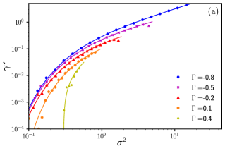
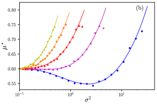
Figure S2: (a) The correlations between elements $a_{ij}$ and $a_{ki}$ [defined in Eq. (LABEL:correlations)] and (b) the scaled mean of the reduced interaction matrix elements [see Eq. (S98)]. The remaining system parameters are $\mu=0.6$, $N=4000$ and the results represented by points were averaged over 10 trials.

S6.2 Non-Gaussian statistics

Let us now consider some of the higher-order statistics of the reduced interaction matrix that are relevant for the calculation of the eigenvalue spectrum. For example, consider the quantity

$$S_{3}=\frac{1}{(\phi N)^{2}}\sum_{ijkl}\overline{(a_{ik}-\mu^{\prime}/N_{{}_{\mathcal{S}}})(a_{kl}-\mu^{\prime}/N_{{}_{\mathcal{S}}})(a_{lj}-\mu^{\prime}/N_{{}_{\mathcal{S}}})\theta_{i}\theta_{j}\theta_{k}\theta_{l}},$$ (S102)

This can be related to the quantities that appear in the series for the resolvent in Eq. (S37)

$$S_{3} =-i\frac{1}{(\phi N)^{2}}\sum_{(ijkl)}\left\langle\frac{1}{A}\frac{\delta^{3}A}{\delta\lambda_{ik}\delta\lambda_{kl}\delta\lambda_{lj}}\right\rangle\bigg{|}_{\lambda=0}$$

$$+\phi^{3}\mu^{3}-(\mu^{\prime})^{3}-3\phi^{2}\mu^{2}\mu^{\prime}+3(\mu^{\prime})^{3}+(\phi\mu-\mu^{\prime})\left[(\mu^{\prime})^{2}+\gamma^{\prime}+2\phi\sigma^{2}\Gamma+2(\mu^{\prime})^{2}\right],$$ (S103)

where we have

$$-i\frac{1}{(\phi N)^{2}} \sum_{(ijkl)}\left\langle\frac{1}{A}\frac{\delta^{3}A}{\delta\lambda_{ik}\delta\lambda_{kl}\delta\lambda_{lj}}\right\rangle\bigg{|}_{\lambda=0}=\frac{\sigma^{4}}{\phi}\bigg{[}(1+\Gamma)\sigma^{2}\Gamma\chi\chi_{2}M^{2}+(1+\Gamma)\Gamma q\chi_{{}_{T}}^{2}\sigma^{2}\chi$$

$$+\chi_{{}_{T}}M\Gamma^{2}(2\phi+\chi^{2}\Gamma\sigma^{2}+\chi_{2}q\sigma^{2})+\chi_{{}_{T}}M(2\Gamma\phi+\chi^{2}\sigma^{2}+\chi_{2}\Gamma q\sigma^{2})\bigg{]}.$$ (S104)

If the matrix elements $z_{ij}$ (and hence $a^{\prime}_{ij}$) were Gaussian random variables, then the quantity $S_{3}$ would vanish. We see that $S_{3}$ does not vanish, even when the elements of the original interaction matrix are Gaussian random variables (see Fig. S3 below).

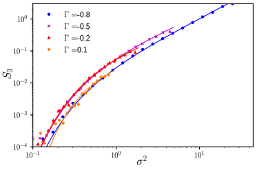
Figure S3: Demonstrating that the statistics of the reduced interaction matrix elements are non-Gaussian. The quantity $S_{3}$ would be zero if $z_{ij}$ were Gaussian random numbers. The remaining system parameters are $\mu=0.6$, $N=4000$ and the results represented by points were averaged over 10 trials. The results for $\Gamma=0.4$ are too small to be visible.

References

Mézard et al. (1987)M. Mézard, G. Parisi,
and M. Virasoro, Spin glass theory and beyond: An
Introduction to the Replica Method and Its Applications, Vol. 9 (World Scientific Publishing Company, London, 1987).
Wigner (1958)E. P. Wigner, Annals
of Mathematics 67, 325
(1958).
Wigner (1967)E. P. Wigner, SIAM
Review 9, 1 (1967).
Aljadeff et al. (2015)J. Aljadeff, M. Stern, and T. Sharpee, Physical Review
Letters 114, 088101
(2015).
Kuczala and Sharpee (2016)A. Kuczala and T. O. Sharpee, Physical Review E 94, 050101 (2016).
Coolen et al. (2005)A. C. Coolen, P. Sollich, and R. Kühn, Theory of Neural Information
Processing Systems (Oxford University Press,
Oxford, UK, 2005).
Rajan and Abbott (2006)K. Rajan and L. F. Abbott, Physical Review Letters 97, 188104 (2006).
Louart et al. (2018)C. Louart, Z. Liao, and R. Couillet, The Annals of Applied
Probability 28, 1190
(2018).
Laloux et al. (2000)L. Laloux, P. Cizeau,
M. Potters, and J.-P. Bouchaud, International
Journal of Theoretical and Applied Finance 3, 391 (2000).
Bouchaud and Potters (2008)J.-P. B. Bouchaud and M. Potters, in The Oxford Handbook of Random Matrix Theory (Oxford University Press, Oxford (UK), 2008).
May (1972)R. M. May, Nature 238, 413 (1972).
Allesina and Tang (2012)S. Allesina and S. Tang, Nature 483, 205 (2012).
Opper and Diederich (1992)M. Opper and S. Diederich, Physical Review Letters 69, 1616 (1992).