On the strong convergence of the trajectories of a Tikhonov regularized second order dynamical system with asymptotically vanishing damping

Abstract. This paper deals with a second order dynamical system with vanishing damping that contains a Tikhonov regularization term, in connection to the minimization problem of a convex Fréchet differentiable function $g$. We show that for appropriate Tikhonov regularization parameters the value of the objective function in a generated trajectory converges fast to the global minimum of the objective function and a trajectory generated by the dynamical system converges weakly to a minimizer of the objective function. We also obtain the fast convergence of the velocities towards zero and some integral estimates. Nevertheless, our main goal is to extend and improve some recent results obtained in [6] and [12] concerning the strong convergence of the generated trajectories to an element of minimal norm from the $\operatorname*{argmin}$ set of the objective function $g$. Our analysis also reveals that the damping coefficient and the Tikhonov regularization coefficient are strongly correlated.

Key Words. convex optimization, continuous second order dynamical system, Tikhonov regularization, strong convergence, convergence rate

AMS subject classification. 34G20, 47J25, 90C25, 90C30, 65K10

1 Introduction

Let $\mathcal{H}$ be a Hilbert space endowed with the scalar product $\langle\cdot,\cdot\rangle$ and norm $\|\cdot\|$ and let $g:\mathcal{H}\longrightarrow\mathbb{R}$ be a convex continuously differentiable function whose solution set $\operatorname*{argmin}g$ is nonempty. Assume further, that $\nabla g$ is Lipschitz continuous on bounded sets. Consider the minimization problem

$$(P)\,\,\,\inf_{x\in\mathcal{H}}g(x)$$

in connection to the second order dynamical system

$$\begin{cases}\ddot{x}(t)+\frac{\alpha}{t^{q}}\dot{x}(t)+\nabla g\left(x(t)\right)+\frac{a}{t^{p}}x(t)=0\\ x(t_{0})=u_{0},\,\dot{x}(t_{0})=v_{0},\end{cases}$$ (1)

where $t_{0}>0$, $(u_{0},v_{0})\in\mathcal{H}\times\mathcal{H}$ and $\alpha,\,q,\,a,\,p>0.$

First of all, note that the term $\frac{a}{t^{p}}x(t)$ is a Tikhonov regularization term, which may assure the strong convergence of a generated trajectory to the minimizer of minimal norm of the objective function $g.$ For further insight into the Tikhonov regularization techniques we refer to [8, 11, 10, 12, 17, 18, 20].

The case $q=1$ was intensively studied in the literature. Indeed, in [8] Attouch, Chbani and Riahi showed that for $q=1,$ $p>2,$ $a=1$ and $\alpha>3$ the generated trajectories of (1) converge weakly to a minimizer of $g$. Further, one has $g(x(t)-\min g=o\left(\frac{1}{t^{2}}\right).$ On the other hand, if $p<2$, then the strong convergence result $\liminf_{t\to+\infty}\|x(t)-x^{*}\|=0$ holds, where $x^{*}$ is the element of minimum norm from $\operatorname*{argmin}g.$ The previous result is also true if $p=2$ and $a>\frac{4}{9}\alpha(\alpha-3).$ Similar results have been obtained in [17] and [3] for some second order dynamical systems with (implicit) Hessian driven damping and Tikhonov regularization term (see also [15, 4]). The case $p=2$ seems to be critical in the sense that separates the case when one obtains fast convergence of the function values and weak convergence of the trajectories to a minimizer, and the case when the strong convergence of the trajectories to a minimizer of minimum norm is ensured. However, recently Attouch and László in [12] succeeded to obtain both rapid convergence towards the infimal value of $g$, and the strong convergence of the trajectories towards the element of minimum norm of the set of minimizers of $g.$ More precisely, in [12] it is shown that if $q=1,$ $p=2,$ $a>0$ and $\alpha>3$ then $\displaystyle g\left(x(t)\right)-\min g=O\left(\frac{1}{t^{2}}\right)\mbox{ as }t\to+\infty.$ Further, the trajectory $x$ is bounded, $\displaystyle\|\dot{x}(t)\|=O\left(\frac{1}{t}\right)\mbox{ as }t\to+\infty$, and there is strong convergence to the minimum norm solution $x^{*}$, i.e. $\liminf_{t\to\infty}{\|x(t)-x^{\ast}\|}=0.$ A similar result has been obtained in [3] for a second order dynamical systems with implicit Hessian driven damping.

We emphasize that for $q=1$ the dynamical system (1) is a Tikhonov regularized version of the second order dynamical system with vanishing damping, studied by Su-Boyd-Candès [25] in connection to the optimization problem $(P)$, that is,

$$\rm{(HBS)}\,\,\,\,\,\ddot{x}(t)+\frac{\alpha}{t}\dot{x}(t)+\nabla g\left(x(t)\right)=0,\,x(t_{0})=u_{0},\,\dot{x}(t_{0})=v_{0},\,u_{0},v_{0}\in\mathcal{H}.$$

It is obvious that the latter system can be obtained from (1) by taking $q=1$ and $a=0$.

According to [25], the trajectories generated by (HBS) assure fast minimization property of order $\mathcal{O}\left(1/t^{2}\right)$ for the decay $g(x(t))-\min g,$ provided $\alpha\geq 3$. For $\alpha>3$, it has been shown by Attouch-Chbani-Peypouquet-Redont [7] that each trajectory generated by (HBS) converges weakly to a minimizer of the objective function $g$. Further, it is shown in [13] and [23] that the asymptotic convergence rate of the values is actually $o(1/t^{2})$.

The case $\alpha=3$ corresponds to Nesterov’s historical algorithm [24] as it was emphasized in [25], more precisely for $\alpha=3$, (HBS) can be seen as a continuous version of the accelerated gradient method of Nesterov, (see also [22]).

However, the case $\alpha=3$ is critical, that is, the convergence of the trajectories generated by (HBS) remains an open problem. The subcritical case $\alpha\leq 3$ has been examined by Apidopoulos-Aujol-Dossal [5] and Attouch-Chbani-Riahi [9], with the convergence rate of the objective values $\displaystyle{\mathcal{O}\Big{(}t^{-\frac{2\alpha}{3}}}\Big{)}$.

When the objective function $g$ is not convex, the convergence of the trajectories generated by (HBS) is a largely open question. Recent progress has been made in [16], where the convergence of the trajectories of a system, which can be considered as a perturbation of (HBS) has been obtained in a non-convex setting. For other results concerning the dynamical system (HBS) and its extensions we refer to [9, 19, 21].

Let us mention that for the particular case $q=\frac{p}{2},$ (1) becomes (TRIGS) the dynamical system introduced recently in [12] and studied further in [6].

Note that in [12] it is shown that for $\frac{2}{3}<p<2,$ $q=\frac{p}{2}$, $\alpha>0$ and $a=1$ a trajectory of the dynamical system (1) satisfies the following: $g(x(t))-\min g=\mathcal{O}\left(\frac{1}{t^{\frac{3p}{2}-1}}\right)$ and $\liminf_{t\to\infty}{\|x(t)-x^{\ast}\|}=0.$

The previous result has been improved in [6], where the authors showed that for $0<q<1,\,p=2q,$ $\alpha>0$ and $a=1$ one has: $\displaystyle g\left(x(t)\right)-\min g=O\left(\frac{1}{t^{2q}}\right)\mbox{ as }t\to+\infty,$ $\displaystyle\|\dot{x}(t)\|=O\left(\frac{1}{t^{\frac{q+1}{2}}}\right)\mbox{ as }t\to+\infty$ and $\lim_{t\to\infty}{\|x(t)-x^{\ast}\|}=0.$ More precisely, by denoting $x_{t}$ the unique minimizer of the strongly convex function $g(x)+\frac{1}{2t^{p}}\|x\|^{2}$, it is shown in [6] that $\|x(t)-x_{t}\|=O\left(\frac{1}{t^{\frac{1-q}{2}}}\right)\mbox{ as }t\to+\infty$ and this implies that

$$\lim_{t\to\infty}{\|x(t)-x^{\ast}\|}=0.$$

The main goal of this paper is to extend and improve the results obtained in [12] and [6] for the general case $0<q<1$ and $p,\alpha,a>0.$ Since our analysis shows that the parameters $q,\,p$ and $a$ are strongly related in order to give a better perspective of the results obtained in this paper, we emphasize the following.

1. If $0<q<1,\,0<p<q+1$ and $x^{*}=\operatorname*{proj}_{\operatorname*{argmin}g}0$ is the minimum norm element from $\operatorname*{argmin}g$, then the following results hold.

   • $\lim\limits_{t\to\infty}\|x(t)-x^{\ast}\|=0.$

   • If $\frac{3q+1}{2}\leq p<q+1$ then $\|\dot{x}(t)\|=O\left(\frac{1}{t^{2q-p+1}}\right)\mbox{ as }t\to+\infty.$ Further, if $\frac{3q+1}{2}\leq p\leq\frac{4q+2}{3}$, then $g(x(t))-\min g=O\left(\frac{1}{t^{p}}\right)\mbox{ as }t\to+\infty$ and for $\frac{4q+2}{3}<p<q+1$ one has $g(x(t))-\min g=O\left(\frac{1}{t^{4q-2p+2}}\right)\mbox{ as }t\to+\infty.$

   • If $0<p<\frac{3q+1}{2}$, then $\|\dot{x}(t)\|=O\left(\frac{1}{t^{\frac{p+1-\max(q,p-q)}{2}}}\right)\mbox{ as }t\to+\infty$ and $g(x(t))-\min g=O\left(\frac{1}{t^{p}}\right)\mbox{ as }t\to+\infty.$

2. If $0<q<1,\,q+1<p<2,$ or $p=2$ and $a\geq q(1-q)$ then the trajectory $x(t)$ is bounded and following results hold.

   • $\displaystyle{\int_{t_{0}}^{+\infty}t^{q}\|\dot{x}(t)\|^{2}dt<+\infty\mbox{ and }\int_{t_{0}}^{+\infty}t^{q}\left(g\left(x(t)\right)-\min g\right)dt<+\infty}.$

   • $\displaystyle{\|\dot{x}(t)\|=o\left(\frac{1}{t^{q}}\right)\mbox{ as }t\to+\infty\mbox{ and }g\left(x(t)\right)-\min g=o\left(\frac{1}{t^{2q}}\right)\mbox{ as }t\to+\infty.}$

   • For every $x^{*}\in\operatorname*{argmin}g$, there exists the limit $\lim_{t\to+\infty}\|x(t)-x^{*}\|.$ Even more, the trajectory $x(t)$ converges weakly, as $t\to+\infty$, to an element of $\operatorname*{argmin}g$.

3. The case $p=q+1$, $0<q<1$ is critical in the sense that separates the cases of weak and strong convergence of the trajectories. In this case we could not obtain any convergence result for the generated trajectories, however we show that some pointwise estimates hold.

Observe that our results considerably extend the results obtained in [6], where only the case $q=\frac{p}{2}$ was considered. Of course for this instance we reobtain the results from [6]. Further, our analysis reveals that the choice $p=2q$ in the dynamical system (1) is not necessarily optimal. Indeed, for a fixed $q$ we may obtain the convergence rate of order $O\left(\frac{1}{t^{\frac{4q+2}{3}}}\right)$ for the decay $g(x(t))-\min g$, meanwhile in [6] only the rate $O\left(\frac{1}{t^{2q}}\right)$ has been obtained. On the other hand, if we fix $p\in]0,2[$, then for every $q\in\left]\max\left(0,\frac{2p-1}{3}\right),1\right[$ one has $g(x(t))-\min g=O\left(\frac{1}{t^{p}}\right),$ hence we can choose infinitely many damping coefficients in order to obtain the same convergence rate as in case $q=\frac{p}{2}.$ These features of our dynamical system (1) will also be underlined via some numerical experiments.

The paper is organized as follows. In the next section we show the weak convergence of the trajectories generated by the dynamical system (1) to a minimizer of the objective function $g.$ Pointwise and integral estimates for the velocity and decay $g\left(x(t)\right)-\min g$ are also obtained. In section 3 we give sufficient conditions that assure the strong convergence of the trajectories generated by the dynamical system (1) to the minimum norm element from $\operatorname*{argmin}g.$ Pointwise estimates are also obtained under the same assumptions. In section 4 we present some numerical experiment in order to give a better insight on the behaviour of a trajectory generated by the dynamical system (1). Finally we conclude our paper by emphasizing some perspectives.

2 Asymptotic analysis of the trajectories generated by the dynamical system (1)

Existence and uniqueness of a $C^{2}([t_{0},+\infty),\mathcal{H})$ global solution of the dynamical system (1) can be shown via the classical Cauchy-Lipschitz-Picard theorem by rewriting (1) as a first order system in the product space $\mathcal{H}\times\mathcal{H}$, see Theorem 10 from Appendix. In this section we carry out the asymptotic analysis concerning the trajectories $x(t)$ generated by the dynamical system (1). A new feature of our analysis is that we provide the integral estimates $\int_{t_{0}}^{+\infty}t^{q}\|\dot{x}(t)\|^{2}dt<+\infty$ and $\int_{t_{0}}^{+\infty}t^{q}\left(g\left(x(t)\right)-\min g\right)dt<+\infty.$ The convergence rates $\|\dot{x}(t)\|=O\left(\frac{1}{t^{q}}\right)\mbox{ as }t\to+\infty$ and $g\left(x(t)\right)-\min g=O\left(\frac{1}{t^{2q}}\right)\mbox{ as }t\to+\infty$ are also obtained and it is shown that the trajectory is bounded. Based on these results we are able to show for every $x^{*}\in\operatorname*{argmin}g$ the existence of the limit $\lim_{t\to+\infty}\|x(t)-x^{*}\|.$ Finally, we obtain ’$o$’ estimates for the decay $g\left(x(t)\right)-\min g$ and the velocity $\|\dot{x}(t)\|$ and we show that a trajectory converges weakly to a minimizer of the objective function $g.$

In the next result we show that pointwise estimates can be obtained in the following general cases.

Theorem 1.

Assume that $0<q<1,$ $\alpha>0$, $0<p\leq 2$ and for $p=2$ one has $a\geq q(1-q)$. Let $t_{0}>0$ and for some starting points $u_{0},v_{0}\in\mathcal{H}$ let $x:[t_{0},\infty)\to\mathcal{H}$ be the unique global solution of (1). Then, the following results hold.

• If $0<q<\frac{p}{2}\leq 1$ then $g\left(x(t)\right)-\min g=O\left(\frac{1}{t^{2q}}\right)\mbox{ as }t\to+\infty\mbox{ and }\|\dot{x}(t)\|=O\left(\frac{1}{t^{q}}\right)\mbox{ as }t\to+\infty.$

• If $\frac{p}{2}\leq q<1$ then $g\left(x(t)\right)-\min g=O\left(\frac{1}{t^{p}}\right)\mbox{ as }t\to+\infty\mbox{ and }\|\dot{x}(t)\|=O\left(\frac{1}{t^{\frac{p}{2}}}\right)\mbox{ as }t\to+\infty.$

Proof .

First, let $x^{\ast}\in\operatorname*{argmin}g$ and consider $b>0$ that will be adjusted later. We denote $g^{\ast}:=g(x^{\ast})=\min g$ and we introduce the energy functional $\mathcal{E}:[t_{0},\infty)\to\mathbb{R}$

$$\mathcal{E}(t)= t^{2q}\left(g(x(t))-g^{\ast}\right)+\frac{a}{2t^{p-2q}}\|x(t)\|^{2}+\frac{1}{2}\|b(x(t)-x^{\ast})+t^{q}\dot{x}(t)\|^{2}+\frac{b(\alpha-b-qt^{q-1})}{2}\|x(t)-x^{*}\|^{2}.$$ (2)

Then,

$$\dot{\mathcal{E}}(t) =2qt^{2q-1}\left(g(x(t))-g^{\ast}\right)+t^{2q}\langle{\nabla}g(x(t)),\dot{x}(t)\rangle$$ (3)

$$+\frac{a(2q-p)t^{2q-p-1}}{2}\|x(t)\|^{2}+at^{2q-p}\langle\dot{x}(t),x(t)\rangle+\langle(b+qt^{q-1})\dot{x}(t)+t^{q}\ddot{x}(t),b(x(t)-x^{\ast})+t^{q}\dot{x}(t)\rangle$$

$$+b(\alpha-b-qt^{q-1})\langle\dot{x}(t),x(t)-x^{*}\rangle+\frac{bq(1-q)t^{q-2}}{2}\|x(t)-x^{*}\|^{2}.$$

From the dynamical system (1), we have that

$$\ddot{x}(t)=-\frac{a}{t^{p}}x(t)-\frac{\alpha}{t^{q}}\dot{x}(t)-\nabla g(x(t)),$$ (4)

hence

$$\langle(b+qt^{q-1})\dot{x}(t)+t^{q}\ddot{x}(t),b(x(t)-x^{\ast})+t^{q}\dot{x}(t)\rangle=$$ (5)

$$\langle(b+qt^{q-1}-\alpha)\dot{x}(t)-at^{q-p}x(t)-t^{q}\nabla g(x(t)),b(x(t)-x^{\ast})+t^{q}\dot{x}(t)\rangle=$$

$$b(b+qt^{q-1}-\alpha)\langle\dot{x}(t),x(t)-x^{*}\rangle+(b+qt^{q-1}-\alpha)t^{q}\|\dot{x}(t)\|^{2}$$

$$-abt^{q-p}\langle x(t),x(t)-x^{*}\rangle-at^{2q-p}\langle\dot{x}(t),x(t)\rangle$$

$$-bt^{q}\langle{\nabla}g(x(t)),x(t)-x^{\ast}\rangle-t^{2q}\langle\nabla g(x(t)),\dot{x}(t)\rangle.$$

Combining (3) and (5) we get

$$\dot{\mathcal{E}}(t) =2qt^{2q-1}\left(g(x(t))-g^{\ast}\right)+(b+qt^{q-1}-\alpha)t^{q}\|\dot{x}(t)\|^{2}+\frac{a(2q-p)t^{2q-p-1}}{2}\|x(t)\|^{2}$$ (6)

$$-bt^{q}\langle{\nabla}g(x(t))+at^{-p}x(t),x(t)-x^{\ast}\rangle+\frac{bq(1-q)t^{q-2}}{2}\|x(t)-x^{*}\|^{2}.$$

Consider now the strongly convex function

$$g_{t}:\mathcal{H}\longrightarrow\mathbb{R},\,g_{t}(x)=g(x)+\frac{a}{2t^{p}}\|x\|^{2}.$$

From the gradient inequality we have

$$g_{t}(y)-g_{t}(x)\geq\langle{\nabla}g_{t}(x),y-x\rangle+\frac{a}{2t^{p}}\|x-y\|^{2},\mbox{ for all }x,y\in\mathcal{H}.$$

Take now $y=x^{*}$ and $x=x(t).$ We get

$$g(x^{*})+\frac{a}{2t^{p}}\|x^{*}\|^{2}-g(x(t))-\frac{a}{2t^{p}}\|x(t)\|^{2}\geq$$

$$-\langle{\nabla}g(x(t))+at^{-p}x(t),x(t)-x^{*}\rangle+\frac{a}{2t^{p}}\|x(t)-x^{*}\|^{2}.$$

Consequently,

$$-bt^{q}\langle{\nabla}g(x(t))+at^{-p}x(t),x(t)-x^{*}\rangle \leq bt^{q}(g(x^{*})-g(x(t)))+\frac{abt^{q-p}}{2}\|x^{*}\|^{2}-\frac{abt^{q-p}}{2}\|x(t)\|^{2}$$ (7)

$$-\frac{abt^{q-p}}{2}\|x(t)-x^{*}\|^{2}.$$

By inserting (7) in (6) we get

$$\dot{\mathcal{E}}(t) =(2qt^{2q-1}-bt^{q})\left(g(x(t))-g^{\ast}\right)+(b+qt^{q-1}-\alpha)t^{q}\|\dot{x}(t)\|^{2}+\frac{a(2q-p)t^{2q-p-1}-abt^{q-p}}{2}\|x(t)\|^{2}$$ (8)

$$+\frac{bq(1-q)t^{q-2}-abt^{q-p}}{2}\|x(t)-x^{*}\|^{2}+\frac{abt^{q-p}}{2}\|x^{*}\|^{2}.$$

Since

$$\frac{1}{2}\|b(x(t)-x^{\ast})+t^{q}\dot{x}(t)\|^{2}\leq b^{2}\|x(t)-x^{*}\|^{2}+t^{2q}\|\dot{x}(t)\|^{2}$$

one has

$$\mathcal{E}(t)\leq t^{2q}\left(g(x(t))-g^{\ast}\right)+\frac{a}{2t^{p-2q}}\|x(t)\|^{2}+t^{2q}\|\dot{x}(t)\|^{2}+\frac{b(\alpha+b-qt^{q-1})}{2}\|x(t)-x^{*}\|^{2}.$$ (9)

Let $r=\max(q,p-q)$ and consider $K>0$ that will be defined in what follows. Now, by multiplying (9) with $\frac{K}{t^{r}}$ and adding to (8) we get

$$\dot{\mathcal{E}}(t)+\frac{K}{t^{r}}\mathcal{E}(t) \leq(2qt^{2q-1}-bt^{q}+Kt^{2q-r})\left(g(x(t))-g^{\ast}\right)+(b+qt^{q-1}-\alpha+Kt^{q-r})t^{q}\|\dot{x}(t)\|^{2}$$ (10)

$$+\frac{a(2q-p)t^{2q-p-1}-abt^{q-p}+aKt^{2q-p-r}}{2}\|x(t)\|^{2}$$

$$+\frac{bq(1-q)t^{q-2}-abt^{q-p}+Kb(\alpha+b-qt^{q-1})t^{-r}}{2}\|x(t)-x^{*}\|^{2}$$

$$+\frac{abt^{q-p}}{2}\|x^{*}\|^{2}.$$

Now, take $0<b<\alpha$ . If $p<2$ consider $0<K<\min\left(b,\alpha-b,\frac{a}{\alpha+b}\right).$ If $p=2$ then by hypotheses we have $a>q(1-q)$, so take $0<K<\min\left(b,\alpha-b,\frac{a-q(1-q)}{\alpha+b}\right).$ Then, easily can be observed that there exists $t_{1}\geq t_{0}$ such that

$$\dot{\mathcal{E}}(t)+\frac{K}{t^{r}}\mathcal{E}(t) \leq\frac{abt^{q-p}}{2}\|x^{*}\|^{2}\mbox{ for all }t\geq t_{1}.$$ (11)

Now, since $r=\max(q,p-q)$ and $0<q<1$ we can take $r=1$ provided $p=q+1.$ In this case, by multiplying (11) with $t^{K}$ we get

$$\frac{d}{dt}\left(t^{K}\mathcal{E}(t)\right)\leq\frac{ab\|x^{*}\|^{2}}{2}t^{K-1}\mbox{ for all }t\geq t_{1}.$$

By integrating the latter relation on an interval $[t_{1},T],\,T>t_{1}$ we conclude that there exists $C>0$ such that

$$T^{K}\mathcal{E}(T)\leq\frac{ab\|x^{*}\|^{2}}{2K}T^{K}+C.$$

Consequently,

$$\mathcal{E}(T)\leq\frac{ab\|x^{*}\|^{2}}{2K}+\frac{C}{T^{K}}\leq C_{1}\mbox{ for some }C_{1}>0,$$

hence for all $t\geq t_{1}$ one has

$$g(x(t))-g^{*}\leq\frac{C_{1}}{t^{2q}}\mbox{ and }\|\dot{x}(t)\|\leq\frac{\sqrt{C_{1}}}{t^{q}}.$$

In other words

$$g(x(t))-g^{*}=O\left(\frac{1}{t^{2q}}\right)\mbox{ and }\|\dot{x}(t)\|=O\left(\frac{1}{t^{q}}\right),\mbox{ as }t\to+\infty.$$ (12)

In the case $r\neq 1$, by multiplying (11) with $e^{\frac{K}{1-r}t^{1-r}}$ we get

$$\frac{d}{dt}\left(e^{\frac{K}{1-r}t^{1-r}}\mathcal{E}(t)\right)\leq\frac{ab\|x^{*}\|^{2}}{2}t^{q-p}e^{\frac{K}{1-r}t^{1-r}}\mbox{ for all }t\geq t_{1}.$$ (13)

Observe further, that for all $t\geq t_{1}$ one has

$$\frac{1}{K}\frac{d}{dt}\left(t^{q-p+r}e^{\frac{K}{1-r}t^{1-r}}\right)=\frac{1}{K}\left((q-p+r)t^{q-p+r-1}+Kt^{q-p}\right)e^{\frac{K}{1-r}t^{1-r}}\geq t^{q-p}e^{\frac{K}{1-r}t^{1-r}}.$$

Combining the latter relation with (13) we get

$$\frac{d}{dt}\left(e^{\frac{K}{1-r}t^{1-r}}\mathcal{E}(t)\right)\leq\frac{ab\|x^{*}\|^{2}}{2K}\frac{d}{dt}\left(t^{q-p+r}e^{\frac{K}{1-r}t^{1-r}}\right)\mbox{ for all }t\geq t_{1}.$$ (14)

By integrating (14) on an interval $[t_{1},T],\,T>t_{1}$ we conclude that

$$e^{\frac{K}{1-r}T^{1-r}}\mathcal{E}(T)\leq C_{1}T^{q-p+r}e^{\frac{K}{1-r}T^{1-r}}+C_{2},$$

where $C_{1}=\frac{ab\|x^{*}\|^{2}}{2K}$ and $C_{2}=e^{\frac{K}{1-r}t_{1}^{1-r}}\mathcal{E}(t_{1})-\frac{ab\|x^{*}\|^{2}}{2K}t_{1}^{q-p+r}e^{\frac{K}{1-r}t_{1}^{1-r}}.$

Consequently,

$$\mathcal{E}(T)\leq C_{1}T^{q-p+r}+\frac{C_{2}}{e^{\frac{K}{1-r}T^{1-r}}}\leq C_{3}T^{q-p+r}\mbox{ for some }C_{3}>0,$$

hence for all $t\geq t_{1}$ one has

$$g(x(t))-g^{*}\leq\frac{C_{3}}{t^{q+p-r}}\mbox{ and }\|\dot{x}(t)\|\leq\frac{\sqrt{C_{3}}}{t^{\frac{q+p-r}{2}}}.$$ (15)

Now, since $r=\max(q,p-q)$ one has $r=q$ if $2q\geq p$ and $r=p-q$ if $p\geq 2q.$

Therefore, in case $q<1$ and $2q\geq p$, (15) leads to

$$g(x(t))-g^{*}=O\left(\frac{1}{t^{p}}\right)\mbox{ and }\|\dot{x}(t)\|=O\left(\frac{1}{t^{\frac{p}{2}}}\right)\mbox{ as }t\to+\infty.$$

Finally, in case $q<1$ and $2q<p,\,p\neq q+1$, (15) leads to

$$g(x(t))-g^{*}=O\left(\frac{1}{t^{2q}}\right)\mbox{ and }\|\dot{x}(t)\|=O\left(\frac{1}{t^{q}}\right)\mbox{ as }t\to+\infty.$$

$\blacksquare$

Remark 2.

Note that, though provides the same convergence rate, the case $p=q+1$ must be treated separately in the proof of Theorem 1. This is due to the fact that in this case $r=1$, hence the antiderivative of $\frac{K}{t^{r}}$ is $K\ln t$ and therefore (11) needs a special attention. Actually, we will show that the case $p=q+1$ is critical, in the sense that separates the cases when the trajectories converge strongly and the trajectories converges weakly, respectively.

Remark 3.

Observe that our analysis also work for the case $q=1$ and $\alpha>3.$ Indeed, in this case by taking $2<b<\alpha-1$ and $0<K<\min\left(b-2,\alpha-1-b,\frac{a}{\alpha+b-1}\right)$ in the proof of Theorem 1 we reobtain some results from [8] and [12]. More precisely if $p\leq 2$ one has

$$g\left(x(t)\right)-\min g=O\left(\frac{1}{t^{p}}\right)\mbox{ as }t\to+\infty\mbox{ and }\|\dot{x}(t)\|=O\left(\frac{1}{t^{\frac{p}{2}}}\right)\mbox{ as }t\to+\infty.$$

Further, if $p\geq 2$ one has

$$g\left(x(t)\right)-\min g=O\left(\frac{1}{t^{2}}\right)\mbox{ as }t\to+\infty\mbox{ and }\|\dot{x}(t)\|=O\left(\frac{1}{t}\right)\mbox{ as }t\to+\infty.$$

In the next result we obtain some integral estimates in case $p>q+1.$

Theorem 4.

Assume that $0<q\leq 1,$ $q+1<p\leq 2$ and for $p=2$ one has $a\geq q(1-q)$. Let $t_{0}>0$ and for some starting points $u_{0},v_{0}\in\mathcal{H}$ let $x:[t_{0},\infty)\to\mathcal{H}$ be the unique global solution of (1). Then, the trajectory $x(t)$ is bounded and following results hold.

(integral estimates)  $\displaystyle{\int_{t_{0}}^{+\infty}t^{q}\|\dot{x}(t)\|^{2}dt<+\infty\mbox{ and }\int_{t_{0}}^{+\infty}t^{q}\left(g\left(x(t)\right)-\min g\right)dt<+\infty}.$

(pointwise estimates) $\displaystyle{\|\dot{x}(t)\|=O\left(\frac{1}{t^{q}}\right)\mbox{ as }t\to+\infty\mbox{ and }g\left(x(t)\right)-\min g=O\left(\frac{1}{t^{2q}}\right)\mbox{ as }t\to+\infty.}$

Proof .

Consider the energy functional defined at (2). According to (8) one has

$$\dot{\mathcal{E}}(t) =(2qt^{2q-1}-bt^{q})\left(g(x(t))-g^{\ast}\right)+(b+qt^{q-1}-\alpha)t^{q}\|\dot{x}(t)\|^{2}+\frac{a(2q-p)t^{2q-p-1}-abt^{q-p}}{2}\|x(t)\|^{2}$$ (16)

$$+\frac{bq(1-q)t^{q-2}-abt^{q-p}}{2}\|x(t)-x^{*}\|^{2}+\frac{abt^{q-p}}{2}\|x^{*}\|^{2}.$$

Now, we take $b<\alpha$ and we conclude that there exist $t_{1}\geq t_{0}$ and $C_{1},C_{2}>0$ such that for all $t\geq t_{1}$ the following hold.

$$\mathcal{E}(t)\geq 0,$$

$$2qt^{2q-1}-bt^{q}\leq-C_{1}t^{q},$$

$$(b+qt^{q-1}-\alpha)t^{q}\leq-C_{2}t^{q}$$

and

$$\frac{a(2q-p)t^{2q-p-1}-abt^{q-p}}{2}\|x(t)\|^{2}+\frac{bq(1-q)t^{q-2}-abt^{q-p}}{2}\|x(t)-x^{*}\|^{2}\leq 0.$$

Consequently,

$$\dot{\mathcal{E}}(t)+C_{1}t^{q}\left(g(x(t))-g^{\ast}\right)+C_{2}t^{q}\|\dot{x}(t)\|^{2}\leq\frac{ab\|x^{*}\|^{2}}{2}\frac{1}{t^{p-q}},\mbox{ for all }t\geq t_{1}.$$ (17)

By integrating (17) on $[t_{1},T],\,T>t_{1}$ and taking into account that by hypotheses we have $p>q+1$, we conclude that there exists $C_{3}>0$ such that

$$\int_{t_{1}}^{T}\dot{\mathcal{E}}(t)dt+C_{1}\int_{t_{1}}^{T}t^{q}\left(g(x(t))-g^{\ast}\right)dt+C_{2}\int_{t_{1}}^{T}t^{q}\|\dot{x}(t)\|^{2}dt \leq\frac{ab\|x^{*}\|^{2}}{2}\int_{t_{1}}^{T}\frac{1}{t^{p-q}}dt$$ (18)

$$\leq\frac{ab\|x^{*}\|^{2}}{2}\int_{t_{1}}^{+\infty}\frac{1}{t^{p-q}}dt\leq C_{3}.$$

Hence, $\mathcal{E}(t)$ is bounded which implies that $x(t)$ is bounded,

$$g(x(t)-g^{*}=O\left(\frac{1}{t^{2q}}\right)\mbox{ as }t\to+\infty$$

and

$$\|\dot{x}(t)\|=O\left(\frac{1}{t^{q}}\right)\mbox{ as }t\to+\infty.$$

Further, (18) ensures that

$$t^{q}\left(g(x(t))-g^{\ast}\right),t^{q}\|\dot{x}(t)\|^{2}\in L^{1}[t_{0},+\infty[.$$ (19)

$\blacksquare$

Remark 5.

Observe that the conclusion of the previous theorem remains valid also in case $q=1,\,p>2$ and $\alpha>3$ and this fact can be seen if one takes $2<b<\alpha-1$ in its proof. However, these results have already been obtained in [8].

Even more, the pointwise estimates remain valid also in the case $q=1$ $p>2$ and $\alpha=3$. Indeed, the result follows if one takes $b=2$ in the proof of Theorem 4, however the integral estimates do not hold anymore.

Now, we are able to show the existence of the limit $\lim_{t\to+\infty}\|x(t)-x^{*}\|.$

Lemma 6.

Assume that $q+1<p\leq 2$ and for $p=2$ one has $a\geq q(1-q).$ For some starting points $u_{0},v_{0}\in\mathcal{H}$ let $x:[t_{0},\infty)\to\mathcal{H}$ be the unique global solution of (1). Let $x^{*}\in\operatorname*{argmin}g.$ Then, there exists the limit $\lim_{t\to+\infty}\|x(t)-x^{*}\|.$

Proof .

The proof is based on Lemma 13. Indeed, for $x^{*}\in\operatorname*{argmin}g$ consider the function $w(t)=\frac{1}{2}\|x(t)-x^{*}\|^{2}.$ Then, by using (1) one has

$$\ddot{w}(t)+\frac{\alpha}{t^{q}}\dot{w}(t)=\left\langle\ddot{x}(t)+\frac{\alpha}{t^{q}}\dot{x}(t),x(t)-x^{*}\right\rangle+\|\dot{x}(t)\|^{2}=\left\langle-{\nabla}g({x}(t))-\frac{a}{t^{p}}{x}(t),x(t)-x^{*}\right\rangle+\|\dot{x}(t)\|^{2}$$

Now, from the monotonicity of ${\nabla}g$ we have $\langle-{\nabla}g({x}(t)),x(t)-x^{*}\rangle\leq 0$ and

$$\left\langle-\frac{a}{t^{p}}{x}(t),x(t)-x^{*}\right\rangle=\frac{a}{2t^{p}}(\|x^{*}\|^{2}-\|x(t)\|^{2}-\|x(t)-x^{*}\|^{2}).$$

Consequently,

$$\ddot{w}(t)+\frac{\alpha}{t^{q}}\dot{w}(t)\leq\frac{a}{2t^{p}}\|x^{*}\|^{2}+\|\dot{x}(t)\|^{2}.$$ (20)

We show that Lemma 13 can be applied with $p(t)=1,\,q(t)=\frac{\alpha}{t^{q}}$ and $k(t)=\frac{a}{2t^{p}}\|x^{*}\|^{2}+\|\dot{x}(t)\|^{2}.$ Note that since $p>q+1$ and according to Theorem 4 it holds that $t^{q}\|\dot{x}(t)\|^{2}\in L^{1}[t_{0},+\infty[,$ we have

$$t^{q}k(t)\in L^{1}[t_{0},+\infty[.$$ (21)

Now, if $0<q<1$ then $\int_{t_{0}}^{t}\frac{q(s)}{p(s)}ds=\frac{\alpha}{1-q}(t^{1-q}-t_{0}^{1-q}),$ hence $\exp\left(\int_{t_{0}}^{t}\frac{q(s)}{p(s)}ds\right)=C_{1}e^{C_{2}t^{1-q}},$ where $C_{1}=e^{-\frac{\alpha}{1-q}t_{0}^{1-q}}$ and $C_{2}=\frac{\alpha}{1-q}.$ Consequently,

$$\frac{1}{\exp\left(\int_{t_{0}}^{t}\frac{q(s)}{p(s)}ds\right)}\in L^{1}[t_{0},+\infty[.$$ (22)

Further

$$\left(\int_{t}^{+\infty}\frac{dT}{\exp\left(\int_{t_{0}}^{T}\frac{q(s)}{p(s)}ds\right)}\right)\frac{\exp\left(\int_{t_{0}}^{t}\frac{q(s)}{p(s)}ds\right)}{p(t)}k(t)=\int_{t}^{+\infty}e^{-C_{2}T^{1-q}}dTe^{C_{2}t^{1-q}}k(t).$$ (23)

Consider the integral $I_{t}=\int_{t}^{+\infty}e^{-C_{2}T^{1-q}}dT.$ By substituting $C_{2}T^{1-q}=\theta$ we obtain $T=C_{2}^{-\frac{1}{1-q}}\theta^{\frac{1}{1-q}},$ hence $dT=C_{3}\theta^{\frac{q}{1-q}}d\theta,$ where $C_{3}=\frac{C_{2}^{-\frac{1}{1-q}}}{1-q}.$ Consequently,

$$I_{t}=C_{3}\int_{C_{2}t^{1-q}}^{+\infty}\theta^{\frac{q}{1-q}}e^{-\theta}d\theta=C_{3}\Gamma\left(\frac{1}{1-q},C_{2}t^{1-q}\right),$$

where $\Gamma(s,x)=\int_{x}^{+\infty}\theta^{s-1}e^{-\theta}d\theta$ is the upper incomplete gamma function. It is well known (see [2]) that

$$\frac{\Gamma(s,x)}{x^{s-1}e^{-x}}\to 1\mbox{ as }x\to+\infty.$$

Consequently,

$$\frac{\Gamma\left(\frac{1}{1-q},C_{2}t^{1-q}\right)}{(C_{2}t^{1-q})^{\frac{q}{1-q}}e^{-C_{2}t^{1-q}}}\to 1,\mbox{ as }t\to+\infty,$$

which shows that there exists $C_{4}>0$ such that

$$\int_{t}^{+\infty}e^{-C_{2}T^{1-q}}dTe^{C_{2}t^{1-q}}\leq C_{4}t^{q}.$$

Now, combining the previous relation with (21) and (23) we obtain that

$$\left(\int_{t}^{+\infty}\frac{dT}{\exp\left(\int_{t_{0}}^{T}\frac{q(s)}{p(s)}ds\right)}\right)\frac{\exp\left(\int_{t_{0}}^{t}\frac{q(s)}{p(s)}ds\right)}{p(t)}k(t)\leq C_{4}t^{q}k(t)\in L^{1}[t_{0},+\infty[.$$ (24)

Hence, according to Lemma 13, there exists the limit $\lim_{t\to+\infty}\|x(t)-x^{*}\|.$ $\blacksquare$

In the next results we obtain ’$o$’ estimates for the decay $g(x(t))-\min g$ and the velocity $\dot{x}(t),$ further we show that a trajectory generated by the dynamical system (1) converges weakly to a minimizer of the objective function $g.$

Theorem 7.

Assume that $q+1<p\leq 2$ and for $p=2$ one has $a\geq q(1-q).$ Let $t_{0}>0$ and for some starting points $u_{0},v_{0}\in\mathcal{H}$ let $x:[t_{0},\infty)\to\mathcal{H}$ be the unique global solution of (1). Then, the trajectory $x(t)$ converges weakly, as $t\to+\infty$, to an element of $\operatorname*{argmin}g$. Further, one has

$${\|\dot{x}(t)\|=o\left(\frac{1}{t^{q}}\right)\mbox{ as }t\to+\infty\mbox{ and }g\left(x(t)\right)-\min g=o\left(\frac{1}{t^{2q}}\right)\mbox{ as }t\to+\infty.}$$

Proof .

By using the same notations as in the proof of Theorem 4, in what follows we show that there exists

$$\lim_{t\to+\infty}\left(t^{2q}\left(g(x(t))-g^{\ast}\right)+\frac{t^{2q}}{2}\|\dot{x}(t)\|^{2}\right)\in\mathbb{R}.$$

Now, according to (2) one has

$$\dot{\mathcal{E}}(t) =2qt^{2q-1}\left(g(x(t))-g^{\ast}\right)+t^{2q}\langle{\nabla}g(x(t)),\dot{x}(t)\rangle$$ (25)

$$+\frac{d}{dt}\left(\frac{a}{2t^{p-2q}}\|x(t)\|^{2}+\frac{1}{2}\|b(x(t)-x^{\ast})+t^{q}\dot{x}(t)\|^{2}+\frac{b(\alpha-b-qt^{q-1})}{2}\|x(t)-x^{*}\|^{2}\right).$$

Further, by using (1) we get

$$t^{2q}\langle{\nabla}g(x(t)),\dot{x}(t)\rangle =-t^{2q}\langle\ddot{x}(t),\dot{x}(t)\rangle-\alpha t^{q}\|\dot{x}(t)\|^{2}-at^{2q-p}\langle x(t),\dot{x}(t)\rangle$$ (26)

$$=-\frac{d}{dt}\left(\frac{t^{2q}}{2}\|\dot{x}(t)\|^{2}\right)+qt^{2q-1}\|\dot{x}(t)\|^{2}-\alpha t^{q}\|\dot{x}(t)\|^{2}$$

$$-a\frac{d}{dt}\left(\frac{t^{2q-p}}{2}\|x(t)\|^{2}\right)+a\frac{2q-p}{2}t^{2q-p-1}\|x(t)\|^{2}.$$

Combining (25), (26) and (17) we get

$$\frac{d}{dt}\left(-\frac{t^{2q}}{2}\|\dot{x}(t)\|^{2}+\frac{1}{2}\|b(x(t)-x^{\ast})+t^{q}\dot{x}(t)\|^{2}+\frac{b(\alpha-b-qt^{q-1})}{2}\|x(t)-x^{*}\|^{2}\right)\leq$$ (27)

$$-2qt^{2q-1}\left(g(x(t))-g^{\ast}\right)+(\alpha t^{q}-qt^{2q-1})\|\dot{x}(t)\|^{2}-a\frac{2q-p}{2}t^{2q-p-1}\|x(t)\|^{2}+\frac{ab\|x^{*}\|^{2}}{2}\frac{1}{t^{p-q}}.$$

Since $q>2q-1$, $2q-p-1<q-p<-1$ and $x(t)$ is bounded, further, $t^{q}\left(g(x(t))-g^{\ast}\right),t^{q}\|\dot{x}(t)\|^{2}\in L^{1}[t_{0},+\infty[$, we get that the right hand side of (27) is of class $L^{1}[t_{0},+\infty[$. Hence, by Lemma 11 there exists the limit

$$\lim_{t\to+\infty}\left(-\frac{t^{2q}}{2}\|\dot{x}(t)\|^{2}+\frac{1}{2}\|b(x(t)-x^{\ast})+t^{q}\dot{x}(t)\|^{2}+\frac{b(\alpha-b-qt^{q-1})}{2}\|x(t)-x^{*}\|^{2}\right)\in\mathbb{R}.$$

Now according to Lemma 6 there exists $\lim_{t\to+\infty}\|x(t)-x^{*}\|\in\mathbb{R},$ consequently there exists the limit

$$\lim_{t\to+\infty}t^{q}\langle x(t)-x^{\ast},\dot{x}(t)\rangle\in\mathbb{R}.$$ (28)

According to (17) one has $\dot{\mathcal{E}}(t)\leq\frac{ab\|x^{*}\|^{2}}{2}\frac{1}{t^{p-q}},\mbox{ for all }t\geq t_{1}$ and, since $p>q+1$, the right hand side of the previous inequality is of class $L^{1}[t_{0},+\infty[.$ Consequently Lemma 11 assures the existence and finiteness of the limit

$$\lim_{t\to+\infty}\mathcal{E}(t)=$$

$$\lim_{t\to+\infty}\left(t^{2q}\left(g(x(t))-g^{\ast}\right)+\frac{a}{2t^{p-2q}}\|x(t)\|^{2}+\frac{1}{2}\|b(x(t)-x^{\ast})+t^{q}\dot{x}(t)\|^{2}+\frac{b(\alpha-b-qt^{q-1})}{2}\|x(t)-x^{*}\|^{2}\right).$$

Obviously $p>q+1>2q$ and the fact that $x(t)$ is bounded assure that $\lim_{t\to+\infty}\frac{a}{2t^{p-2q}}\|x(t)\|^{2}=0.$ Further the existence of $\lim_{t\to+\infty}\|x(t)-x^{*}\|$ and (28) implies that there exists the limit

$$\lim_{t\to+\infty}\left(t^{2q}\left(g(x(t))-g^{\ast}\right)+\frac{t^{2q}}{2}\|\dot{x}(t)\|^{2}\right)\in\mathbb{R}.$$ (29)

According to (19) we have

$$\int_{t_{0}}^{+\infty}\frac{1}{t^{q}}\left(t^{2q}\left(g(x(t))-g^{\ast}\right)+\frac{t^{2q}}{2}\|\dot{x}(t)\|^{2}\right)dt=\int_{t_{0}}^{+\infty}t^{q}\left(g(x(t))-g^{\ast}\right)dt+\int_{t_{0}}^{+\infty}\frac{t^{q}}{2}\|\dot{x}(t)\|^{2}dt<+\infty.$$ (30)

Now, since $\frac{1}{t^{q}}\not\in L^{1}[t_{0},+\infty[$ from (29) and (30) we obtain that

$$\lim_{t\to+\infty}\left(t^{2q}\left(g(x(t))-g^{\ast}\right)+\frac{t^{2q}}{2}\|\dot{x}(t)\|^{2}\right)=0,$$

hence,

$$g(x(t))-g^{\ast}=o\left(\frac{1}{t^{2q}}\right)\mbox{ and }\|\dot{x}(t)\|=o\left(\frac{1}{t^{q}}\right).$$

Next we show that $x(t)$ converges weakly to a minimizer of $g.$ According to Lemma 6, for every $x^{*}\in\operatorname*{argmin}g$ the limit $\lim_{t\to+\infty}\|x(t)-x^{*}\|$ exists. Now, if $\overline{x}\in\mathcal{H}$ is a weak sequential limit point of $x(t)$ then there exists a sequence $(t_{n})_{n\in\mathbb{N}}\subseteq[t_{0},+\infty[$ such that $\lim_{n\to+\infty}t_{n}=+\infty$ and $x(t_{n})$ converges weakly to $\overline{x}$ as $n\to+\infty.$ Obviously the function $g$ is weakly lower semicontinuous, since it is convex and continuous, consequently $g(\overline{x})\leq\liminf_{n\to+\infty}g(x(t_{n})=\lim_{n\to+\infty}g(x(t_{n})=g^{*}=\min g$, which shows that $\overline{x}\in\operatorname*{argmin}g.$ According to the Opial lemma it follows that

$$w-\lim_{t\to+\infty}x(t)\in\operatorname*{argmin}g.$$

$\blacksquare$

3 Strong convergence

We continue the present section by emphasizing the main idea behind the Tikhonov regularization, which will generate strong convergence results for our dynamical system (1) to a minimizer of the objective function of minimal norm. By $x_{t}$ we denote the unique solution of the strongly convex minimization problem

$$\min_{x\in\mathcal{H}}\left(g(x)+\frac{a}{2t^{p}}\|x\|^{2}\right).$$

We know, (see for instance [10]), that the Tikhonov approximation curve $t\to x_{t}$ satisfies $x^{\ast}=\lim\limits_{t\to+\infty}x_{t}$, where $x^{\ast}=\operatorname*{argmin}\limits_{x\in\operatorname*{argmin}g}\|x\|$ is the minimal norm element from the set $\operatorname*{argmin}g.$ Obviously, $\{x^{*}\}=\operatorname*{proj}_{\operatorname*{argmin}g}0$ and we have the inequality $\|x_{t}\|\leq\|x^{\ast}\|$ (see [17]).

Since $x_{t}$ is the unique minimum of the strongly convex function $g_{t}(x)=g(x)+\frac{a}{2t^{p}}\|x\|^{2},$ obviously one has

$${\nabla}g_{t}(x_{t})={\nabla}g(x_{t})+\frac{a}{t^{p}}x_{t}=0.$$ (31)

Further, according to Lemma 2 from [6] the function $t\longrightarrow x_{t}$ is derivable almost everywhere and one has

$$\left\|\frac{d}{dt}x_{t}\right\|\leq\frac{p}{t}\|x_{t}\|\mbox{ for almost every}t\geq t_{0}.$$ (32)

Note that since $g_{t}$ is strongly convex, from the gradient inequality we have

$$g_{t}(y)-g_{t}(x)\geq\langle{\nabla}g_{t}(x),y-x\rangle+\frac{a}{2t^{p}}\|x-y\|^{2},\mbox{ for all }x,y\in\mathcal{H}.$$ (33)

In particular

$$g_{t}(x)-g_{t}(x_{t})\geq\frac{a}{2t^{p}}\|x-x_{t}\|^{2},\mbox{ for all }x\in\mathcal{H}.$$ (34)

Let $y:[t_{0},+\infty[\to\mathcal{H},s\longrightarrow y(s)$ derivable at a point $t\in]t_{0},+\infty[.$ Then it is obvious that

$$\frac{d}{dt}g_{t}(y(t))=\langle{\nabla}g_{t}(y(t)),\dot{y}(t)\rangle-\frac{ap}{2t^{p+1}}\|y(t)\|^{2}.$$ (35)

Finally, for all $x,y\in\mathcal{H}$, one has

$$g(x)-g(y)=(g_{t}(x)-g_{t}(x_{t}))+(g_{t}(x_{t})-g_{t}(y))+\frac{a}{2t^{p}}(\|y\|^{2}-\|x\|^{2})\leq g_{t}(x)-g_{t}(x_{t})+\frac{a}{2t^{p}}\|y\|^{2}.$$ (36)

Now, in order to show the strong convergence of the dynamical system (1) to an element of minimum norm of the nonempty, convex and closed set $\operatorname*{argmin}g$, we state our main result of the present section.

Theorem 8.

Assume that $0<q<1,\,0<p<q+1$ and let $x$ be the unique global solution of (1). Let $x^{*}=\operatorname*{proj}_{\operatorname*{argmin}g}0.$ Then, $\lim\limits_{t\to\infty}\|x(t)-x^{\ast}\|=0$ and the following estimates hold.

• If $\frac{3q+1}{2}\leq p<q+1$ then $\|\dot{x}(t)\|=O\left(\frac{1}{t^{2q-p+1}}\right)\mbox{ as }t\to+\infty.$
  Further, if $\frac{3q+1}{2}\leq p\leq\frac{4q+2}{3}$, then $g(x(t))-\min g=O\left(\frac{1}{t^{p}}\right)\mbox{ as }t\to+\infty$ and for $\frac{4q+2}{3}<p<q+1$ one has $g(x(t))-\min g=O\left(\frac{1}{t^{4q-2p+2}}\right)\mbox{ as }t\to+\infty.$

• If $0<p<\frac{3q+1}{2}$, then $\|\dot{x}(t)\|=O\left(\frac{1}{t^{\frac{p+1-\max(q,p-q)}{2}}}\right)\mbox{ as }t\to+\infty.$
  Further, $g(x(t))-\min g=O\left(\frac{1}{t^{p}}\right)\mbox{ as }t\to+\infty.$

Proof .

Consider $\alpha>b>0$ and define, for every $t\geq t_{0}$, the following energy functional

$$E(t) =t^{2q}(g_{t}(x(t))-g_{t}(x_{t}))+\frac{1}{2}\|b(x(t)-x_{t})+t^{q}\dot{x}(t)\|^{2}+\frac{b(\alpha-b-qt^{q-1})}{2}\|x(t)-x_{t}\|^{2}.$$ (37)

Obviously, there exists $t_{1}\geq t_{0}$ such that $\frac{b(\alpha-b-qt^{q-1})}{2}>0$ for all $t\geq t_{1}$, hence $E(t)\geq 0$ for all $t\geq t_{1}.$ Now, by using (35) and the fact that ${\nabla}g_{t}(x_{t})=0$ we get

$$\dot{E}(t) =2qt^{2q-1}(g_{t}(x(t))-g_{t}(x_{t}))+t^{2q}\left(\langle{\nabla}g_{t}(x(t)),\dot{x}(t)\rangle-\frac{ap}{2t^{p+1}}\|x(t)\|^{2}+\frac{ap}{2t^{p+1}}\|x_{t}\|^{2}\right)$$ (38)

$$+\left\langle b\left(\dot{x}(t)-\frac{d}{dt}x_{t}\right)+qt^{q-1}\dot{x}(t)+t^{q}\ddot{x}(t),b(x(t)-x_{t})+t^{q}\dot{x}(t)\right\rangle$$

$$+\frac{b(q(1-q)t^{q-2})}{2}\|x(t)-x_{t}\|^{2}+b(\alpha-b-qt^{q-1})\left\langle\dot{x}(t)-\frac{d}{dt}x_{t},x(t)-x_{t}\right\rangle.$$

Proceeding as in (5) we obtain

$$\langle(b+qt^{q-1})\dot{x}(t)+t^{q}\ddot{x}(t),b(x(t)-x_{t})+t^{q}\dot{x}(t)\rangle=b(b+qt^{q-1}-\alpha)\langle\dot{x}(t),x(t)-x_{t}\rangle$$ (39)

$$+(b+qt^{q-1}-\alpha)t^{q}\|\dot{x}(t)\|^{2}-bt^{q}\langle{\nabla}g_{t}(x(t)),x(t)-x_{t}\rangle-t^{2q}\langle\nabla g_{t}(x(t)),\dot{x}(t)\rangle.$$

Now, according to (33) one has

$$-bt^{q}(g_{t}(x(t))-g_{t}(x_{t}))-\frac{ab}{2t^{p-q}}\|x(t)-x_{t}\|^{2}\geq bt^{q}\langle{\nabla}g_{t}(x(t)),x_{t}-x(t)\rangle$$ (40)

Combining (38), (39) and (40) we get

$$\dot{E}(t) \leq(2qt^{2q-1}-bt^{q})(g_{t}(x(t))-g_{t}(x_{t}))-\frac{ap}{2t^{p-2q+1}}\left(\|x(t)\|^{2}-\|x_{t}\|^{2}\right)$$ (41)

$$+(b+qt^{q-1}-\alpha)t^{q}\|\dot{x}(t)\|^{2}+\frac{b(q(1-q)t^{q-2}-at^{q-p})}{2}\|x(t)-x_{t}\|^{2}$$

$$+b(\alpha-qt^{q-1})\left\langle\frac{d}{dt}x_{t},x(t)-x_{t}\right\rangle+bt^{q}\left\langle\frac{d}{dt}x_{t},\dot{x}(t)\right\rangle$$

Observe further, that

$$\frac{1}{2}\|b(x(t)-x_{t})+t^{q}\dot{x}(t)\|^{2}\leq b^{2}\|x(t)-x_{t}\|^{2}+t^{2q}\|\dot{x}(t)\|^{2},$$

hence, we have

$$E(t) \leq t^{2q}(g_{t}(x(t))-g_{t}(x_{t}))+t^{2q}\|\dot{x}(t)\|^{2}+\frac{b(\alpha+b-qt^{q-1})}{2}\|x(t)-x_{t}\|^{2}.$$ (42)

Consider now $r=\max(q,p-q)$ and $K>0$ that will be defined later. Then, (41) and (42) lead to

$$\dot{E}(t)+\frac{K}{t^{r}}E(t) \leq(2qt^{2q-1}-bt^{q}+Kt^{2q-r})(g_{t}(x(t))-g_{t}(x_{t}))-\frac{ap}{2t^{p-2q+1}}\left(\|x(t)\|^{2}-\|x_{t}\|^{2}\right)$$ (43)

$$+(b+qt^{q-1}-\alpha+Kt^{q-r})t^{q}\|\dot{x}(t)\|^{2}$$

$$+\frac{b(q(1-q)t^{q-2}-at^{q-p}+(\alpha+b-qt^{q-1})Kt^{-r})}{2}\|x(t)-x_{t}\|^{2}$$

$$+b(\alpha-qt^{q-1})\left\langle\frac{d}{dt}x_{t},x(t)-x_{t}\right\rangle+bt^{q}\left\langle\frac{d}{dt}x_{t},\dot{x}(t)\right\rangle,\mbox{ for all }t\geq t_{1}.$$

Now, it is obvious that for every $\beta>0$ one has

$$\left\langle\frac{d}{dt}x_{t},x(t)-x_{t}\right\rangle\leq\frac{\beta}{2}t^{p-q}\left\|\frac{d}{dt}x_{t}\right\|^{2}+\frac{1}{2\beta}t^{q-p}\|x(t)-x_{t}\|^{2}.$$

By using (32) and the fact that there exists $t_{2}\geq t_{1}$ such that $b(\alpha-qt^{q-1})>0$ for all $t\geq t_{2}$, we obtain that

$$b(\alpha-qt^{q-1})\left\langle\frac{d}{dt}x_{t},x(t)-x_{t}\right\rangle\leq\frac{\beta p^{2}b(\alpha-qt^{q-1})}{2}t^{p-q-2}\left\|x_{t}\right\|^{2}+\frac{b(\alpha-qt^{q-1})}{2\beta}t^{q-p}\|x(t)-x_{t}\|^{2},$$ (44)

for all $t\geq t_{2}$ and every $\beta>0.$

Further, by using (32) again, we obtain that for every $\gamma>0$ it holds

$$bt^{q}\left\langle\frac{d}{dt}x_{t},\dot{x}\right\rangle\leq bt^{q}\left(\frac{p^{2}}{4\gamma t^{2}}\left\|x_{t}\right\|^{2}+\gamma\|\dot{x}(t)\|^{2}\right),\mbox{ for all }t\geq t_{2}.$$ (45)

We recall that $\|x_{t}\|\leq\|x^{*}\|$, hence by injecting (44) and (45) in (43) and neglecting the non-positive term $-\frac{ap}{2t^{p-2q+1}}\|x(t)\|^{2}$ we obtain

$$\dot{E}(t)+\frac{K}{t^{r}}E(t) \leq(2qt^{2q-1}-bt^{q}+Kt^{2q-r})(g_{t}(x(t))-g_{t}(x_{t}))$$ (46)

$$+(b+qt^{q-1}-\alpha+Kt^{q-r}+b\gamma)t^{q}\|\dot{x}(t)\|^{2}$$

$$+\frac{b\left(q(1-q)t^{q-2}-at^{q-p}+(\alpha+b-qt^{q-1})Kt^{-r}+\frac{\alpha-qt^{q-1}}{\beta}t^{q-p}\right)}{2}\|x(t)-x_{t}\|^{2}$$

$$+\left(\frac{ap}{2}t^{2q-p-1}+\frac{\beta p^{2}b(\alpha-qt^{q-1})}{2}t^{p-q-2}+\frac{bp^{2}}{4\gamma}t^{q-2}\right)\|x^{*}\|^{2},\mbox{ for all }t\geq t_{2}\mbox{ and }\beta,\gamma>0.$$

Since $0<b<\alpha$ one can consider $0<\gamma<\frac{\alpha}{b}-1$ and $\beta>\frac{\alpha}{a}.$ Further, choose $K$ such that

$$0<K<\min\left(b,\alpha-b(1+\gamma),\frac{a\beta-\alpha}{\beta(\alpha+b)}\right).$$

Then, easily can be checked that there exists $t_{3}\geq t_{2}$ such that

$$\dot{E}(t)+\frac{K}{t^{r}}E(t)\leq\left(\frac{ap}{2}t^{2q-p-1}+\frac{\beta p^{2}b(\alpha-qt^{q-1})}{2}t^{p-q-2}+\frac{bp^{2}}{4\gamma}t^{q-2}\right)\|x^{*}\|^{2},\mbox{ for all }t\geq t_{3}.$$ (47)

From now on we treat the two cases (i) and (ii) separately.

(i) If $p\geq\frac{3q+1}{2}$, then since by the hypotheses one has $0<q<1$ we conclude that there exists $C>0$ and $t_{4}\geq t_{3}$ such that

$$\left(\frac{ap}{2}t^{2q-p-1}+\frac{\beta p^{2}b(\alpha-qt^{q-1})}{2}t^{p-q-2}+\frac{bp^{2}}{4\gamma}t^{q-2}\right)\|x^{*}\|^{2}\leq Ct^{p-q-2},\mbox{ for all }t\geq t_{4}.$$

Consequently, (47)becomes

$$\dot{E}(t)+\frac{K}{t^{r}}E(t)\leq Ct^{p-q-2},\mbox{ for all }t\geq t_{4}.$$ (48)

Since $0<q<1$ and $q+1>p\geq\frac{3q+1}{2}$ we get that $r=\max(q,p-q)=p-q<1$. By multiplying (48) with $e^{\frac{K}{1-r}t^{1-r}}$ we get

$$\frac{d}{dt}\left(e^{\frac{K}{1-r}t^{1-r}}E(t)\right)\leq Ct^{p-q-2}e^{\frac{K}{1-r}t^{1-r}},\mbox{ for all }t\geq t_{4}.$$ (49)

Observe that

$$\frac{d}{dt}\left(t^{p-q-2+r}e^{\frac{K}{1-r}t^{1-r}}\right)=((p-q-2+r)t^{p-q-3+r}+Kt^{p-q-2})e^{\frac{K}{1-r}t^{1-r}}$$

and since $p<q+1$ and $r<1$ we conclude that

$$\frac{d}{dt}\left(t^{p-q-2+r}e^{\frac{K}{1-r}t^{1-r}}\right)\geq Kt^{p-q-2}e^{\frac{K}{1-r}t^{1-r}},\mbox{ for all }t\geq t_{4}.$$

Hence, (49) becomes

$$\frac{d}{dt}\left(e^{\frac{K}{1-r}t^{1-r}}E(t)\right)\leq\frac{C}{K}\frac{d}{dt}\left(t^{p-q-2+r}e^{\frac{K}{1-r}t^{1-r}}\right),\mbox{ for all }t\geq t_{4}.$$ (50)

Now, by integrating (50) on an interval $[t_{4},T],\,T>t_{4}$ we obtain

$$e^{\frac{K}{1-r}T^{1-r}}E(T)\leq C_{1}T^{p-q-2+r}e^{\frac{K}{1-r}T^{1-r}}+C_{2},$$

where $C_{1}=\frac{C}{K}$ and $C_{2}=e^{\frac{K}{1-r}t_{4}^{1-r}}E(t_{4})-C_{1}t_{4}^{p-q-2+r}e^{\frac{K}{1-r}t_{4}^{1-r}}.$ In other words

$$E(t)\leq C_{1}t^{p-q-2+r}+\frac{C_{2}}{e^{\frac{K}{1-r}t^{1-r}}},\mbox{ for all }t\geq t_{4}.$$

Obviously $\frac{C_{2}}{e^{\frac{K}{1-r}t^{1-r}}}\leq t^{p-q-2+r}$ if $t$ is big enough, hence there exists $t_{5}\geq t_{4}$ and $C_{3}>0$ such that

$$E(t)\leq C_{3}t^{p-q-2+r},\mbox{ for all }t\geq t_{5}.$$ (51)

Taking into account that $r=p-q$ and the definition of $E(t)$, from (51) we obtain at once that

$$\|x(t)-x_{t}\|=O\left(\frac{1}{t^{q-p+1}}\right)\mbox{ as }t\to+\infty.$$ (52)

Now, since $\lim_{t\to+\infty}x_{t}=x^{*}$ from (52) we get

$$\lim_{t\to+\infty}\|x(t)-x^{*}\|=0.$$

Further, (51) leads to

$$\|\dot{x}(t)\|=O\left(\frac{1}{t^{2q-p+1}}\right)\mbox{ as }t\to+\infty$$

and

$$g_{t}(x(t))-g_{t}(x_{t})=O\left(\frac{1}{t^{4q-2p+2}}\right)\mbox{ as }t\to+\infty.$$

Now, if $4q-2p+2\geq p$, that is, $\frac{3q+1}{2}\leq p\leq\frac{4q+2}{3}$, from (36) we obtain that

$$g(x(t))-\min g=O\left(\frac{1}{t^{p}}\right)\mbox{ as }t\to+\infty.$$

Conversely, if $4q-2p+2<p$, that is, $\frac{4q+2}{3}<p<q+1$, from (36) we obtain

$$g(x(t))-\min g=O\left(\frac{1}{t^{4q-2p+2}}\right)\mbox{ as }t\to+\infty.$$

(ii) Let us return now to (47). If $p<\frac{3q+1}{2}$ we conclude that $q+1>p$, hence $t^{2q-p-1}\geq t^{q-2}$ and $t^{2q-p-1}>t^{p-q-2}.$ From the latter relation we deduce that there exists $C>0$ and $t_{4}\geq t_{3}$ such that

$$\left(\frac{ap}{2}t^{2q-p-1}+\frac{\beta p^{2}b(\alpha-qt^{q-1})}{2}t^{p-q-2}+\frac{bp^{2}}{4\gamma}t^{q-2}\right)\|x^{*}\|^{2}\leq Ct^{2q-p-1},\mbox{ for all }t\geq t_{4}.$$

Consequently, (47) becomes

$$\dot{E}(t)+\frac{K}{t^{r}}E(t)\leq Ct^{2q-p-1},\mbox{ for all }t\geq t_{4}.$$ (53)

Observe that $r<1$, hence proceeding analogously as in the previous case we obtain that there exists $C_{1}>0$ and $t_{5}\geq t_{4}$ such that

$$E(t)\leq C_{4}t^{2q-p-1+r},\mbox{ for all }t\geq t_{5}.$$ (54)

Hence, we obtain at once that

$$\|\dot{x}(t)\|^{2}=O\left(\frac{1}{t^{p+1-r}}\right)\mbox{ as }t\to+\infty$$

and

$$g_{t}(x(t))-g_{t}(x_{t})=O\left(\frac{1}{t^{p+1-r}}\right)\mbox{ as }t\to+\infty.$$

Now, from (36) and the fact that $r<1$ we obtain

$$g(x(t))-\min g=O\left(\frac{1}{t^{p}}\right)\mbox{ as }t\to+\infty.$$

Now, if $p\geq 2q$ we have $r=p-q$ hence $2q-p-1+r=q-1<0$ then, according to (37) and (51) one has

$$\frac{b(\alpha-b-qt^{q-1})}{2}\|x(t)-x_{t}\|^{2}\leq C_{4}t^{q-1},\mbox{ for all }t\geq t_{6}.$$

Consequently,

$$\|x(t)-x_{t}\|=O\left(\frac{1}{t^{\frac{1-q}{2}}}\right)\mbox{ as }t\to+\infty.$$ (55)

Conversely, if $p<2q$ then $r=q$, and since $E(t)\geq t^{2q}(g_{t}(x(t))-g_{t}(x_{t}))$ from (54) and (34) we get

$$\frac{at^{2q-p}}{2}\|x(t)-x_{t}\|^{2}\leq C_{4}t^{2q-p-1+r},\mbox{ for all }t\geq t_{5}.$$

Hence,

$$\|x(t)-x_{t}\|=O\left(\frac{1}{t^{\frac{1-q}{2}}}\right)\mbox{ as }t\to+\infty.$$ (56)

Now, since $\lim_{t\to+\infty}x_{t}=x^{*}$ from (55) and (56) we get

$$\lim_{t\to+\infty}\|x(t)-x^{*}\|=0.$$

$\blacksquare$

Remark 9.

Observe that our analysis presented in the proof of Theorem 8 also works for the cases $p=q+1$ and $q=1,\,p\leq 2$, unfortunately one can not obtain an improvement of the results already presented at Theorem 1 and Remark 3.

4 Numerical experiments

In this section we consider two numerical experiments for the trajectories generated by the dynamical system (1) for a convex but not strongly convex objective function

$$g:\mathbb{R}^{2}\to\mathbb{R},\,\,\,g(x,y)=(mx+ny)^{2}\mbox{ where }m,n\in\mathbb{R}\setminus\{0\}.$$

Observe that $\operatorname*{argmin}g=\left\{\left(x,-\frac{m}{n}x\right):x\in\mathbb{R}\right\}$ and $\min g=0$. Obviously, the minimizer of minimal norm of $g$ is $x^{*}=(0,0).$ In the following numerical experiments we consider the starting points $x(1)=(1,1),\,\dot{x}(1)=(-1,-1)$ and the continuous time dynamical system (1) is solved numerically with the ode45 adaptive method in MATLAB on the interval $[1,100]$.

In our first experiment we take $m=5$ and $n=1$, values for which the function $g$ is well conditioned. Further, we consider $\alpha=3.5$, $a=1$ and $p=1.2$ and we study the evolution of the two errors $\|x(t)-x^{*}\|$ and $g(x(t))-\min g$, for a trajectory $x(t)$ generated by the dynamical system (1), with different values of $q$. The results are depicted on Figure 1, where the $y$ axis is endowed with a logarithmic scale.

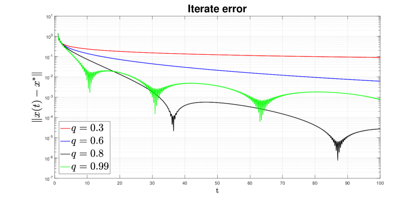
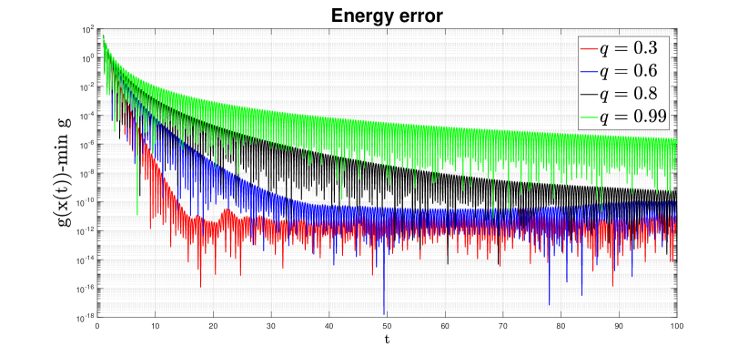
Figure 1: Error analysis with different damping parameters in the dynamical system (1) for a well conditioned convex objective function.

Note that the according to our numerical experiment for $p=1.2$ the best convergence result for the iterate error $\|x(t)-x^{*}\|$ is achieved for $q=0.99$, meanwhile the best best convergence result for the energy error $g(x(t))-\min g$ is attained for $q=0.3.$

In our second experiment we fix $q=0.7$ and we take different values of $p.$ The other parameters remain unchanged. The results are depicted on Figure 2, where the $y$ axis is endowed with a logarithmic scale.

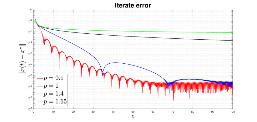
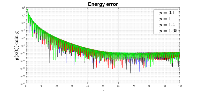
Figure 2: Error analysis with different Tikhonov regularization parameters in the dynamical system (1) for a well conditioned convex objective function.

We conclude that also for fixed damping, one obtains the best convergence behaviour for the iterate error $\|x(t)-x^{*}\|$ for the cases when $p$ is considerably less than $2q.$ Further, one can easily observe that the energy error $g(x(t))-\min g$ is not very sensitive for the changes of the Tikhonov regularization parameter.

Appendix A Appendix

A.1 Existence and uniqueness for the Cauchy problem

Let us first show that the solution for (1) is well posed.

Theorem 10.

Given $(x_{0},v_{0})\in\mathcal{H}\times\mathcal{H}$, there exists a unique global classical solution $x:[t_{0},+\infty[\to\mathcal{H}$ of the dynamical system (1).

Proof .

The proof relies on the combination of the Cauchy-Lipschitz theorem with energy estimates. First consider the Hamitonian formulation of (1) as the first order system

$$\begin{cases}\dot{x}(t)-y(t)=0\vspace{1mm}\\ \dot{y}(t)+\frac{\alpha}{t^{q}}y(t)+\nabla g\left(x(t)\right)+\frac{a}{t^{p}}x(t)=0\vspace{1mm}\\ x(t_{0})=u_{0},\,y(t_{0})=v_{0}.\end{cases}$$ (57)

Taking into account the hypotheses and by applying the Cauchy-Lipschitz theorem in the locally Lipschitz case, we obtain the existence and uniqueness of a local solution. Then, in order to pass from a local solution to a global solution, we rely on the energy estimate obtained by taking the scalar product of (1) with $\dot{x}(t)$. It gives

$$\frac{d}{dt}\left(\frac{1}{2}\|\dot{x}(t)\|^{2}+g(x(t))+\frac{a}{2t^{p}}\|x(t)\|^{2}\right)+\frac{\alpha}{t^{q}}\|\dot{x}(t)\|^{2}+\frac{ap}{2t^{p+1}}\|x(t)\|^{2}=0.$$

Obviously, the energy function $t\mapsto W(t)$ is decreasing where

$$W(t):=\frac{1}{2}\|\dot{x}(t)\|^{2}+g(x(t))+\frac{a}{2t^{p}}\|x(t)\|^{2}.$$

The end of the proof follows a standard argument. Take a maximal solution defined on an interval $[t_{0},T_{\max}[$. If $T_{\max}$ is infinite, the proof is over. Otherwise, if $T_{\max}$ is finite, according to the above energy estimate, we have that $\|\dot{x}(t)\|$ remains bounded. Let $\|\dot{x}_{\infty}\|=\sup_{t\in[t_{0},T_{\max})}\|\dot{x}(t)\|.$ Since $\|x(t)-x(t^{\prime})\|\leq\|\dot{x}_{\infty}\||t-t^{\prime}|$, we get that $\lim_{t\to T_{\max}}x(t):=x_{\infty}\in\mathcal{H}$. By (1) the map $\ddot{x}$ is also bounded on the interval $[t_{0},T_{\max})$ and under the same argument as before $\lim_{t\to T_{\max}}\dot{x}(t):=x_{\infty}$ exists. Applying the local existence theorem with initial data $(x_{\infty},\dot{x}_{\infty})$, we can extend the maximal solution to a strictly larger interval, a clear contradiction. Hence $T_{\max}=+\infty,$ which completes the proof. $\blacksquare$

Appendix B Auxiliary results

In this appendix, we collect some lemmas and technical results which we will use in the analysis of the dynamical system (1).

The following statement is the continuous counterpart of a convergence result of quasi-Fejér monotone sequences. For its proofs we refer to [1, Lemma 5.1].

Lemma 11.

Suppose that $F:[t_{0},+\infty)\rightarrow\mathbb{R}$ is locally absolutely continuous and bounded from below and that there exists $G\in L^{1}([t_{0},+\infty))$ such that

$$\frac{d}{dt}F(t)\leq G(t)$$

for almost every $t\in[t_{0},+\infty)$. Then there exists $\lim_{t\longrightarrow+\infty}F(t)\in\mathbb{R}$.

The continuous version of the Opial Lemma (see [7]) is the main tool for proving weak convergence for the generated trajectory.

Lemma 12.

Let $S\subseteq\mathcal{H}$ be a nonempty set and $x:[t_{0},+\infty)\to H$ a given map such that:

$$(i)\quad\mbox{for every }z\in S\ \mbox{the limit}\ \lim\limits_{t\longrightarrow+\infty}\|x(t)-z\|\ \mbox{exists};$$

$$(ii)\quad\text{every weak sequential limit point of }x(t)\text{ belongs to the set }S.$$

Then the trajectory $x(t)$ converges weakly to an element in $S$ as $t\to+\infty$.

Inspired from [14] Lemma A.6, we have the following result.

Lemma 13.

Let $t_{0}>0$, and let $w:[t_{0},+\infty[\to\mathbb{R}$ be a continuously differentiable function which is bounded from below. Consider $p,q,k:[t_{0},+\infty[\to\mathbb{R}$ nonnegative functions and assume that the function $\frac{1}{\exp\left(\int_{t_{0}}^{t}\frac{q(s)}{p(s)}ds\right)}\in L^{1}(t_{0},+\infty[$ and $\left(\int_{t}^{+\infty}\frac{dT}{\exp\left(\int_{t_{0}}^{T}\frac{q(s)}{p(s)}ds\right)}\right)\frac{\exp\left(\int_{t_{0}}^{t}\frac{q(s)}{p(s)}ds\right)}{p(t)}k(t)\in L^{1}(t_{0},+\infty[.$ Assume further, that

$$p(t)\ddot{w}(t)+q(t)\dot{w}(t)\leq k(t)$$ (58)

for some $\alpha>0$, almost every $t>t_{0}$. Then, the positive part $[\dot{w}]_{+}$ of $\dot{w}$ belongs to $L^{1}(t_{0},+\infty[$, and $\lim_{t\to+\infty}w(t)$ exists.

Proof .

By multiplying (58) with $\frac{1}{p(t)}\exp\left(\int_{t_{0}}^{t}\frac{q(s)}{p(s)}ds\right)$ we get

$$\frac{d}{dt}\left[\exp\left(\int_{t_{0}}^{t}\frac{q(s)}{p(s)}ds\right)\dot{w}(t)\right]\leq\frac{1}{p(t)}\exp\left(\int_{t_{0}}^{t}\frac{q(s)}{p(s)}ds\right)k(t).$$

By integrating the above relation on an interval $[t_{0},T]$ we obtain

$$\exp\left(\int_{t_{0}}^{T}\frac{q(s)}{p(s)}ds\right)\dot{w}(T)\leq\dot{w}(t_{0})+\int_{t_{0}}^{T}\frac{1}{p(t)}\exp\left(\int_{t_{0}}^{t}\frac{q(s)}{p(s)}ds\right)k(t)dt.$$ (59)

Consequently,

$$[\dot{w}]_{+}(T)\leq\frac{|\dot{w}(t_{0})|}{\exp\left(\int_{t_{0}}^{T}\frac{q(s)}{p(s)}ds\right)}+\frac{\int_{t_{0}}^{T}\frac{1}{p(t)}\exp\left(\int_{t_{0}}^{t}\frac{q(s)}{p(s)}ds\right)k(t)dt}{\exp\left(\int_{t_{0}}^{T}\frac{q(s)}{p(s)}ds\right)},$$ (60)

hence

$$\int_{t_{0}}^{+\infty}[\dot{w}]_{+}(T)dT\leq\int_{t_{0}}^{+\infty}\frac{|\dot{w}(t_{0})|}{\exp\left(\int_{t_{0}}^{T}\frac{q(s)}{p(s)}ds\right)}dT+\int_{t_{0}}^{+\infty}\frac{\int_{t_{0}}^{T}\frac{1}{p(t)}\exp\left(\int_{t_{0}}^{t}\frac{q(s)}{p(s)}ds\right)k(t)dt}{\exp\left(\int_{t_{0}}^{T}\frac{q(s)}{p(s)}ds\right)}dT.$$ (61)

Now, from the hypotheses we have

$$\int_{t_{0}}^{+\infty}\frac{|\dot{w}(t_{0})|}{\exp\left(\int_{t_{0}}^{T}\frac{q(s)}{p(s)}ds\right)}dT<+\infty.$$

According to Fubini’s theorem

$$\int_{t_{0}}^{+\infty}\frac{\int_{t_{0}}^{T}\frac{1}{p(t)}\exp\left(\int_{t_{0}}^{t}\frac{q(s)}{p(s)}ds\right)k(t)dt}{\exp\left(\int_{t_{0}}^{T}\frac{q(s)}{p(s)}ds\right)}dT=\int_{t_{0}}^{+\infty}\left(\int_{t}^{+\infty}\frac{dT}{\exp\left(\int_{t_{0}}^{T}\frac{q(s)}{p(s)}ds\right)}\right)\frac{\exp\left(\int_{t_{0}}^{t}\frac{q(s)}{p(s)}ds\right)}{p(t)}k(t)dt.$$

But, according to the hypotheses

$$\int_{t_{0}}^{+\infty}\left(\int_{t}^{+\infty}\frac{dT}{\exp\left(\int_{t_{0}}^{T}\frac{q(s)}{p(s)}ds\right)}\right)\frac{\exp\left(\int_{t_{0}}^{t}\frac{q(s)}{p(s)}ds\right)}{p(t)}k(t)dt<+\infty,$$

consequently

$$\int_{t_{0}}^{+\infty}[\dot{w}]_{+}(T)dT<+\infty.$$

This implies that $\lim_{t\to+\infty}w(t)$ exists. $\blacksquare$

References

- [1] B. Abbas, H. Attouch, B.F. Svaiter, Newton-like dynamics and forward-backward methods for structured monotone inclusions in Hilbert spaces, Journal of Optimization Theory and its Applications 161(2), 331-360, 2014
- [2] M. Abramowitz, I.A. Stegun, eds. (1983) [June 1964]. Handbook of Mathematical Functions with Formulas, Graphs, and Mathematical Tables. Applied Mathematics Series. Vol. 55 (Ninth reprint with additional corrections of tenth original printing with corrections (December 1972); first ed.). Washington D.C.; New York: United States Department of Commerce, National Bureau of Standards; Dover Publications. ISBN 978-0-486-61272-0
- [3] C.D. Alecsa, S.C. László, Tikhonov regularization of a perturbed heavy ball system with vanishing damping, Siam J. Optim., 31(4), 2921-2954, 2021
- [4] C.D. Alecsa, S.C. László, T. Pinţa, An Extension of the Second Order Dynamical System that Models Nesterov’s Convex Gradient Method, Applied Mathematics and Optimization 84(2), 1687–1716, 2021
- [5] V. Apidopoulos, J.-F. Aujol, Ch. Dossal, Convergence rate of inertial Forward-Backward algorithm beyond Nesterov’s rule, Mathematical Programming 180, 137-156, 2020
- [6] H. Attouch, A. Balhag, Z. Chbani, H. Riahi, Damped inertial dynamics with vanishing Tikhonov regularization: Strong asymptotic convergence towards the minimum norm solution, Journal of Differential Equations 311, 29-58, 2022
- [7] H. Attouch, Z. Chbani, J. Peypouquet, P. Redont, Fast convergence of inertial dynamics and algorithms with asymptotic vanishing viscosity, Mathematical Programming 168(1-2) Ser. B, 123-175, 2018
- [8] H. Attouch, Z. Chbani, H. Riahi, Combining fast inertial dynamics for convex optimization with Tikhonov regularization, Journal of Mathematical Analysis and Applications 457(2), 1065-1094, 2018
- [9] H. Attouch, Z. Chbani, H. Riahi, Rate of convergence of the Nesterov accelerated gradient method in the subcritical case . ESAIM-COCV 25, Article number 2, 34 pp., 2019
- [10] H. Attouch, R. Cominetti, A dynamical approach to convex minimization coupling approximation with the steepest descent method, Journal of Differential Equations 128(2), 519-540, 1996
- [11] H. Attouch, M.-O. Czarnecki, Asymptotic Control and Stabilization of Nonlinear Oscillators with Non-isolated Equilibria, J. Differential Equations 179, 278-310, 2002
- [12] H. Attouch, S.C. László, Convex optimization via inertial algorithms with vanishing Tikhonov regularization: fast convergence to the minimum norm solution, https://arxiv.org/abs/2104.11987, 2021
- [13] H. Attouch, J. Peypouquet, The rate of convergence of Nesterov’s accelerated forward-backward method is actually faster than , SIAM J. Optim. 26(3), 1824-1834, 2016
- [14] H. Attouch, J. Peypouquet, Convergence of inertial dynamics and proximal algorithms governed by maximal monotone operators, Mathematical Programming 174(1-2), 391–432, 2019
- [15] H. Attouch, J. Peypouquet, P. Redont, Fast convex optimization via inertial dynamics with Hessian driven damping, Journal of Differential Equations 261(10), 5734-5783, 2016
- [16] R.I. Boţ, E.R. Csetnek, S.C. László, A second-order dynamical approach with variable damping to nonconvex smooth minimization, Applicable Analysis 99(3), 361-378, 2020
- [17] R.I. Boţ, E.R. Csetnek, S.C. László, Tikhonov regularization of a second order dynamical system with Hessian damping, Mathematical Programming 189(1), 151–186, 2021
- [18] R.I. Boţ, S.M. Grad, D. Meier, M. Staudigl, Inducing strong convergence of trajectories in dynamical systems associated to monotone inclusions with composite structure, Adv. Nonlinear Anal. 10, 450–476, 2021
- [19] A. Cabot, H. Engler, S. Gadat, On the long time behavior of second order differential equations with asymptotically small dissipation, Transactions of the American Mathematical Society 361, 5983-6017, 2009
- [20] R. Cominetti, J. Peypouquet, S. Sorin, Strong asymptotic convergence of evolution equations governed by maximal monotone operators with Tikhonov regularization, J. Differential Equations 245, 3753-3763, 2008
- [21] M.A. Jendoubi, R. May, Asymptotics for a second-order differential equation with nonautonomous damping and an integrable source term, Appl. Anal. 94(2), 435–443, 2015
- [22] S.C. László, Convergence rates for an inertial algorithm of gradient type associated to a smooth nonconvex minimization, Mathematical Programming 190(1), 285–329, 2021
- [23] R. May, Asymptotic for a second-order evolution equation with convex potential and vanishing damping term, Turkish Journal of Math. 41(3), 681-685, 2017
- [24] Y. Nesterov, A method of solving a convex programming problem with convergence rate , Soviet Mathematics Doklady 27, 372-376, 1983
- [25] W. Su, S. Boyd, E.J. Candès, A differential equation for modeling Nesterov’s accelerated gradient method: theory and insights, Journal of Machine Learning Research 17(153), 1-43, 2016