Error estimation and adaptivity for stochastic collocation finite elements
Part II: multilevel approximation

Abstract.

A multilevel adaptive refinement strategy for solving linear elliptic partial differential equations with random data is recalled in this work. The strategy extends the a posteriori error estimation framework introduced by Guignard & Nobile in 2018 (SIAM J. Numer. Anal., 56, 3121–3143) to cover problems with a nonaffine parametric coefficient dependence. A suboptimal, but nonetheless reliable and convenient implementation of the strategy involves approximation of the decoupled PDE problems with a common finite element approximation space. Computational results obtained using such a single-level strategy are presented in part I of this work (Bespalov, Silvester & Xu, arXiv:2109.07320). Results obtained using a potentially more efficient multilevel approximation strategy, where meshes are individually tailored, are discussed herein. The codes used to generate the numerical results are available online.

1. Introduction

Partial differential equations (PDEs) with uncertain inputs have provided engineers and scientists with enhanced fidelity in the modelling of real-life phenomena, especially within the last decade. Sparse grid stochastic collocation representations of parametric uncertainty, in combination with finite element discretization of physical space, have emerged as an efficient alternative to Monte-Carlo strategies over this period, especially in the context of nonlinear PDE models or linear PDE problems that are nonlinear in the parameterization of the uncertainty.

The combination of adaptive sparse grid methods with a hierarchy of spatial approximations is a relatively new development, see for example, [12, 13]. In our precursor paper [5] (part I), we extended the adaptive framework developed by Guignard & Nobile [10] and presented a critical comparison of alternative strategies in the context of solving a model problem that combines strong anisotropy in the parametric dependence with singular behavior in the physical space. The numerical results presented in [5] demonstrate the effectivity and robustness of our error estimation strategy as well as the utility of the error indicators guiding the adaptive refinement process. The results in [5] also showed that optimality of convergence is difficult to achieve using a simple single-level approach where a single finite element space is associated with all active collocation points. The main aim of this contribution is to see if optimal convergence rates can be recovered by computing results using a multilevel implementation of the algorithm outlined in [5].

The convergence of a modified version of the adaptive algorithm in [10] has been established by Eigel et al. [7] and independently by Feischl & Scaglioni [9]. The authors of [9] note that the main difficulty in establishing convergence is “the interplay of parametric refinement and finite element refinement”. This interplay is the focus of this contribution.

The model problems that are of interest are stated in section 2. The only difference from the problem statement in [5]  is that we also cover the case where the right-hand side function has a parametric dependence. The adaptive solution algorithm from [5] is extended to cover the case of a non-deterministic right-hand side function in section 3. The novel contribution of this work primarily lies in section 4, where we compare numerical results obtained with our multilevel algorithm with those generated using a single-level strategy and with those computed using the multilevel stochastic Galerkin finite element method (SGFEM).

2. Parametric model problems

Let $D\in\mathbb{R}^{2}$ be a bounded Lipschitz domain with polygonal boundary $\partial D$. Let $\Gamma:=\Gamma_{1}\times\Gamma_{2}\times\cdots\times\Gamma_{M}$ denote the parameter domain in $\mathbb{R}^{M}$, where $M\in\mathbb{N}$ and each $\Gamma_{m}$ ($m=1,\ldots,M$) is a bounded interval in $\mathbb{R}$. We introduce a probability measure $\pi(\mathbf{y}):=\prod_{m=1}^{M}\pi_{m}(y_{m})$ on $(\Gamma,\mathcal{B}(\Gamma))$; here, $\pi_{m}$ denotes a Borel probability measure on $\Gamma_{m}$ ($m=1,\ldots,M$) and $\mathcal{B}(\Gamma)$ is the Borel $\sigma$-algebra on $\Gamma$.

The first model problem is the parametric elliptic problem analyzed in [5]: we seek $u\colon\overline{D}\times\Gamma\to\mathbb{R}$ satisfying

$$\begin{aligned} -\nabla\cdot(a(\cdot,\mathbf{y})\nabla u(\cdot,\mathbf{y}))&=f&&\text{in $D$},\\ u(\cdot,\mathbf{y})&=0&&\text{on $\partial D$,}\end{aligned}$$ (1a)

$$\pi \Gamma u\colon\overline{D}\times\Gamma\to\mathbb{R}$$-almost everywhere on . The second model problem is to find satisfying

$$\begin{aligned} -\nabla^{2}u(\cdot,\mathbf{y}))&=f({\cdot,\mathbf{y}})&&\text{in $D$},\\ u(\cdot,\mathbf{y})&=0&&\text{on $\partial D$,}\end{aligned}$$ (1b)

$\pi$-almost everywhere on $\Gamma$.

In the first model problem, the deterministic right-hand side function $f\in L^{2}(D)$ and the coefficient $a$ is a random field on $(\Gamma,\mathcal{B}(\Gamma),\pi)$ over $L^{\infty}(D)$. In this case we will assume that there exist constants $a_{\min},\,a_{\max}$ such that

$$0<a_{\min}\leq\operatorname*{ess\;inf}_{x\in D}a(x,\mathbf{y})\leq\operatorname*{ess\;sup}_{x\in D}a(x,\mathbf{y})\leq a_{\max}<\infty\quad\text{$\pi$-a.e. on $\Gamma$}.$$ (2)

This assumption implies the following norm equivalence: for any $v\in\mathbb{X}:=H^{1}_{0}(D)$ there holds

$$a_{\min}^{1/2}\|\nabla v\|_{L^{2}(D)}\leq\|a^{1/2}(\cdot,\mathbf{y})\nabla v\|_{L^{2}(D)}\leq a_{\max}^{1/2}\|\nabla v\|_{L^{2}(D)}\quad\text{$\pi$-a.e. on $\Gamma$}.$$ (3)

The parametric problem (1a) is understood in the weak sense: given $f\in L^{2}(D)$, find $u:\Gamma\to\mathbb{X}$ such that

$$\int_{D}a(x,\mathbf{y})\nabla u(x,\mathbf{y})\cdot\nabla v(x)\,\mathrm{d}x=\int_{D}f(x)v(x)\,\mathrm{d}x\quad\forall v\in\mathbb{X},\ \text{$\pi$-a.e. on $\Gamma$}.$$ (4)

The above assumptions on $a$ and $f$ guarantee that the parametric problem (1a) admits a unique weak solution $u$ in the Bochner space $\mathbb{V}:=L_{\pi}^{p}(\Gamma;\mathbb{X})$ for any $p\in[1,\infty]$; see [1, Lemma 1.1] for details. In the sequel, we restrict attention to $p=2$ and denote by $\|\cdot\|$ the norm in $\mathbb{V}=L_{\pi}^{2}(\Gamma;\mathbb{X})$; we also define $\|\cdot\|_{\mathbb{X}}:=\|\nabla\cdot\|_{L^{2}(D)}$.

The second parametric elliptic problem (1b) combines uncertainty in the source term with an isotropic diffusion coefficient field. In this case the right-hand side function $f$ simply needs to be a random field that is smooth enough to ensure that (1b) also admits a unique weak solution $u$ in the Bochner space $\mathbb{V}$.

3. Multilevel stochastic collocation finite element method

Full details of the construction of a multilevel stochastic collocation finite element approximation of the first parametric elliptic problem can be found in [5]. The parametric approximation is associated with a monotone (or, downward-closed) finite set $\Lambda_{\bullet}\subset\mathbb{N}^{M}$ of multi-indices, where $\Lambda_{\bullet}=\{\boldsymbol{\nu}=(\nu_{1},\ldots,\nu_{M}):\nu_{m}\in\mathbb{N},\forall\,m=1,\ldots,M\}$ is such that $\#\Lambda_{\bullet}<\infty$. Each component $\nu_{m}$ ($m=1,\ldots,M$) of the multi-index $\boldsymbol{\nu}\in\Lambda_{\bullet}$ corresponds to a set of collocation points along the $m$th coordinate axis in $\mathbb{R}^{M}$, and the associated sparse grid $\mathcal{Y}_{\bullet}=\mathcal{Y}_{\Lambda_{\bullet}}$ of collocation points on $\Gamma$ is given by

$$\mathcal{Y}_{\Lambda_{\bullet}}:=\bigcup_{\boldsymbol{\nu}\in\Lambda_{\bullet}}\mathcal{Y}^{\,(\boldsymbol{\nu})}={\color[rgb]{0,0,0}\bigcup_{\boldsymbol{\nu}\in\Lambda_{\bullet}}}\,\mathcal{Y}_{1}^{\kappa(\nu_{1})}\times\mathcal{Y}_{2}^{\kappa(\nu_{2})}\times\ldots\times\mathcal{Y}_{M}^{\kappa(\nu_{M})}.$$

Each collocation point $\mathbf{z}\in\mathcal{Y}_{\Lambda_{\bullet}}\subset\Gamma$ is associated with a piecewise linear finite element approximation space $\mathbb{X}_{\bullet\mathbf{z}}=\SS^{1}_{0}(\mathcal{T}_{\bullet\mathbf{z}})$ defined on a mesh $\mathcal{T}_{\bullet\mathbf{z}}$ and an enhanced space $\widehat{\mathbb{X}}_{\bullet\mathbf{z}}$ defined on the mesh $\widehat{\mathcal{T}}_{\bullet\mathbf{z}}$ obtained by uniform refinement of $\mathcal{T}_{\bullet\mathbf{z}}$. The spatial detail space $\mathbb{Y}_{\bullet\mathbf{z}}$ is the approximation space associated with the newly introduced (mid-edge) nodes, i.e., $\widehat{\mathbb{X}}_{\bullet\mathbf{z}}=\mathbb{X}_{\bullet\mathbf{z}}\oplus\mathbb{Y}_{\bullet\mathbf{z}}$. We assume that any finite element mesh employed for the spatial discretization is obtained by (uniform or local) refinement of a given (coarse) initial mesh $\mathcal{T}_{0}$.

The SC-FEM approximation of the solution $u$ to either of the parametric problems (1a) or (1b) is given by

$$u_{\bullet}^{\rm SC}:=\sum\limits_{\mathbf{z}\in\mathcal{Y}_{\bullet}}u_{\bullet\mathbf{z}}(x)L_{\bullet\mathbf{z}}(\mathbf{y}),$$ (5)

where $u_{\bullet\mathbf{z}}\in\mathbb{X}_{\bullet\mathbf{z}}$ are Galerkin approximations satisfying (6a) or (6b) for $\mathbf{z}\in\mathcal{Y}_{\bullet}$, and $\{L_{\bullet\mathbf{z}}(\mathbf{y})=L_{\mathbf{z}}^{\mathcal{Y}_{\bullet}}(\mathbf{y}):\mathbf{z}\in\mathcal{Y}_{\bullet}\}$ is a set of multivariable Lagrange basis functions associated with $\mathcal{Y}_{\bullet}$ and satisfying $L_{\bullet\mathbf{z}}(\mathbf{z}^{\prime})=\delta_{\mathbf{z}\mathbf{z}^{\prime}}$ for any $\mathbf{z},\,\mathbf{z}^{\prime}\in\mathcal{Y}_{\bullet}$. The enhancement of the parametric component of the SC-FEM approximation (5) is done by enriching the index set $\Lambda_{\bullet}$ with multi-indices selected from the reduced margin set ${\rm R}_{\bullet}={\rm R}({\Lambda_{\bullet}})$; this corresponds to adding some collocation points from the set $\widehat{\mathcal{Y}}_{\bullet}\setminus\mathcal{Y}_{\bullet}$, where $\widehat{\mathcal{Y}}_{\bullet}:=\mathcal{Y}_{\Lambda_{\bullet}\cup{\rm R}(\Lambda_{\bullet})}$.

To keep the discussion concise we simply summarize the components of the adaptive refinement strategy. The three components are:

• solution of a deterministic finite element problem at each sparse grid collocation point. That is, the computation of $u_{\bullet\mathbf{z}}\in\mathbb{X}_{\bullet\mathbf{z}}$ satisfying either

  $$\int_{D}a(x,\mathbf{z})\nabla u_{\bullet\mathbf{z}}(x)\cdot\nabla v(x)\,\mathrm{d}x=\int_{D}f(x)v(x)\,\mathrm{d}x\quad\forall v\in\mathbb{X}_{\bullet\mathbf{z}}$$ (6a)

  in the case of the first parametric problem (1a), or

  $$\int_{D}\nabla u_{\bullet\mathbf{z}}(x)\cdot\nabla v(x)\,\mathrm{d}x=\int_{D}f(x,\mathbf{z})v(x)\,\mathrm{d}x\quad\forall v\in\mathbb{X}_{\bullet\mathbf{z}}$$ (6b)

  in the case of the second parametric problem (1b). The enhanced Galerkin solution satisfying (6a) or (6b) for all $v\in\widehat{\mathbb{X}}_{\bullet\mathbf{z}}$ is denoted by $\widehat{u}_{\bullet\mathbf{z}}\in\widehat{\mathbb{X}}_{\bullet\mathbf{z}}$.

• computation of the spatial hierarchical error indicators. For each $\mathbf{z}\in\mathcal{Y}_{\bullet}$, we define $\mu_{\bullet\mathbf{z}}:=\|e_{\bullet\mathbf{z}}\|_{\mathbb{X}}$, where $e_{\bullet\mathbf{z}}\in\mathbb{Y}_{\bullet\mathbf{z}}$ satisfies

  $$\begin{split}\int_{D}\nabla e_{\bullet\mathbf{z}}(x)\cdot\nabla v(x)\,\mathrm{d}x&=\int_{D}f(x)v(x)\,\mathrm{d}x\\ &\quad-\int_{D}a(x,\mathbf{z})\nabla u_{\bullet\mathbf{z}}(x)\cdot\nabla v(x)\,\mathrm{d}x\quad\forall v\in\mathbb{Y}_{\bullet\mathbf{z}}\end{split}$$ (7a)

  in the case of the first parametric problem (1a), or satisfies

  $$\begin{split}\int_{D}\nabla e_{\bullet\mathbf{z}}(x)\cdot\nabla v(x)\,\mathrm{d}x&=\int_{D}f(x,\mathbf{z})v(x)\,\mathrm{d}x\\ &\quad-\int_{D}\nabla u_{\bullet\mathbf{z}}(x)\cdot\nabla v(x)\,\mathrm{d}x\quad\forall v\in\mathbb{Y}_{\bullet\mathbf{z}}\end{split}$$ (7b)

  in the case of the second parametric problem (1b); the corresponding local error indicators $\mu_{\bullet\mathbf{z}}(\xi)$ associated with interior edge midpoints $\xi\in\mathcal{N}_{\bullet\mathbf{z}}^{+}$ are given by components of the solution vector to the linear system stemming from the discrete formulation (7a) or (7b).

• computation of the parametric error indicators

  $$\widetilde{\tau}_{\bullet\boldsymbol{\nu}}=\sum\limits_{\mathbf{z}^{\prime}\in\widetilde{\mathcal{Y}}_{\bullet\boldsymbol{\nu}}}{\color[rgb]{0,0,0}\bigg{\|}u_{0\mathbf{z}^{\prime}}-\sum\limits_{\mathbf{z}\in\mathcal{Y}_{\bullet}}u_{0\mathbf{z}}L_{\bullet\mathbf{z}}(\mathbf{z}^{\prime})\bigg{\|}_{\mathbb{X}}}\,\|\widehat{L}_{\bullet\mathbf{z}^{\prime}}\|_{L_{\pi}^{{\color[rgb]{0,0,0}2}}(\Gamma)}\quad\forall\boldsymbol{\nu}\in{\color[rgb]{0,0,0}({\Lambda_{\bullet}})}{\color[rgb]{0,0,0},}$$ (8)

  where $\widetilde{\mathcal{Y}}_{\bullet\boldsymbol{\nu}}\subset\widehat{\mathcal{Y}}_{\bullet}\setminus\mathcal{Y}_{\bullet}$ are the collocation points ‘generated’ by the multi-index $\boldsymbol{\nu}\in{\rm R}({\Lambda_{\bullet}})$, the functions $u_{0\mathbf{z}^{\prime}}\in\mathbb{X}_{0\mathbf{z}^{\prime}}$ for $\mathbf{z}^{\prime}\in\widetilde{\mathcal{Y}}_{\bullet\boldsymbol{\nu}}$ and $u_{0\mathbf{z}}\in\mathbb{X}_{0\mathbf{z}}$ for $\mathbf{z}\in\mathcal{Y}_{\bullet}$ are Galerkin approximations on some meshes $\mathcal{T}_{0\mathbf{z}^{\prime}}$ and $\mathcal{T}_{0\mathbf{z}}$, respectively, that are to be specified (e.g., $u_{0\mathbf{z}}$ satisfies (6a) or (6b) with $\mathbb{X}_{\bullet\mathbf{z}}$ replaced by $\mathbb{X}_{0\mathbf{z}}$), and $\widehat{L}_{\bullet\mathbf{z}^{\prime}}(\mathbf{y})=L_{\mathbf{z}^{\prime}}^{\widehat{\mathcal{Y}}_{\bullet}}(\mathbf{y})$ denotes the Lagrange polynomial basis function associated with the point $\mathbf{z}^{\prime}\in\widehat{\mathcal{Y}}_{\bullet}$ satisfying $\widehat{L}_{\bullet\mathbf{z}^{\prime}}(\mathbf{z}^{\prime\prime})=\delta_{\mathbf{z}^{\prime}\mathbf{z}^{\prime\prime}}$ for any $\mathbf{z}^{\prime},\,\mathbf{z}^{\prime\prime}\in\widehat{\mathcal{Y}}_{\bullet}$.

We emphasize that the computation of parametric error indicators according to (8) is in line with the hierarchical a posteriori error estimation strategy developed in [5] (see section 4 therein). In the standard single-level SC-FEM setting discussed in [5, section 5], the meshes $\mathcal{T}_{0\mathbf{z}^{\prime}}$ and $\mathcal{T}_{0\mathbf{z}}$ underlying the Galerkin approximations $u_{0\mathbf{z}^{\prime}}$ and $u_{0\mathbf{z}}$ in (8) are all selected to be identical to the (single) finite element mesh $\mathcal{T}_{\bullet\mathbf{z}}=\mathcal{T}_{\bullet}$ that underlies the current SC-FEM solution $u_{\bullet}^{\rm SC}$ in (5). In this case, the indicators in (8) are written as

$$\widetilde{\tau}_{\bullet\boldsymbol{\nu}}=\sum\limits_{\mathbf{z}^{\prime}\in\widetilde{\mathcal{Y}}_{\bullet\boldsymbol{\nu}}}\|u_{\bullet\mathbf{z}^{\prime}}-u_{\bullet}^{\rm SC}(\cdot,\mathbf{z}^{\prime})\|_{\mathbb{X}}\,\|\widehat{L}_{\bullet\mathbf{z}^{\prime}}\|_{L_{\pi}^{{\color[rgb]{0,0,0}2}}(\Gamma)}\quad\forall\boldsymbol{\nu}\in{\rm R}({\Lambda_{\bullet}}),$$

where $u_{\bullet\mathbf{z}^{\prime}}\in\mathbb{X}_{\bullet\mathbf{z}^{\prime}}=\SS^{1}_{0}(\mathcal{T}_{\bullet})$ for all $\mathbf{z}^{\prime}\in\widetilde{\mathcal{Y}}_{\bullet\boldsymbol{\nu}}$ and for all $\boldsymbol{\nu}\in{\rm R}({\Lambda_{\bullet}})$.

In the multilevel SC-FEM setting presented in the adaptive algorithm below, the meshes underlying Galerkin approximations for different collocation points might be different. In this case, when computing the parametric error indicators in (8), the meshes $\mathcal{T}_{0\mathbf{z}^{\prime}}$ ($\mathbf{z}^{\prime}\in\widetilde{\mathcal{Y}}_{\bullet\boldsymbol{\nu}}$) and $\mathcal{T}_{0\mathbf{z}}$ ($\mathbf{z}\in\mathcal{Y}_{\bullet}$) are all selected to be identical to the coarsest finite element mesh $\mathcal{T}_{0}$.

With the above ingredients in place, the solution to the problems in section 2 can be generated using the iterative strategy described in Algorithm 1 together with the marking strategy in Algorithm 2.

Algorithm 1.

Input: $\Lambda_{0}=\{\boldsymbol{1}\}$; $\mathcal{T}_{0\mathbf{z}}:=\mathcal{T}_{0}$ for all $\mathbf{z}\in\widehat{\mathcal{Y}}_{0}=\mathcal{Y}_{\Lambda_{0}\cup{\rm R}(\Lambda_{0})}$; marking criterion.
Set the iteration counter $\ell:=0$, the output counter $k$ and the tolerance.

• Compute Galerkin approximations $\big{\{}u_{\ell\mathbf{z}}\in\mathbb{X}_{\ell\mathbf{z}}:\mathbf{z}\in\widehat{\mathcal{Y}}_{\ell}\big{\}}$ by solving (6a) or (6b).

• Compute spatial error indicators $\big{\{}\mu_{\ell\mathbf{z}}=\|e_{\ell\mathbf{z}}\|_{\mathbb{X}}:\mathbf{z}\in\mathcal{Y}_{\ell}\big{\}}$ by solving (7a) or (7b).

• Compute the parametric error indicators $\big{\{}\widetilde{\tau}_{\ell\boldsymbol{\nu}}:\boldsymbol{\nu}\in{\color[rgb]{0,0,0}({\Lambda_{\ell})}}\big{\}}$ given by (8).

• Use a marking criterion to determine $\mathcal{M}_{\ell\mathbf{z}}\subseteq\mathcal{N}_{\ell\mathbf{z}}^{+}$ for all $\mathbf{z}\in\mathcal{Y}_{\ell}$ and $\Upsilon_{\ell}\subseteq{\color[rgb]{0,0,0}({\Lambda_{\ell})}}$.

• For all $\mathbf{z}\in\mathcal{Y}_{\ell}$, set $\mathcal{T}_{(\ell+1)\mathbf{z}}:=\operatorname*{refine}(\mathcal{T}_{\ell\mathbf{z}},\mathcal{M}_{\ell\mathbf{z}})$.

• Set $\Lambda_{\ell+1}:=\Lambda_{\ell}\cup\Upsilon_{\ell}$, run Algorithm 3 for each $\mathbf{z}^{\prime}\in\mathop{\cup}\limits_{\boldsymbol{\nu}\in\Upsilon_{\ell}}\widetilde{\mathcal{Y}}_{\ell\boldsymbol{\nu}}$ to construct meshes $\mathcal{T}_{(\ell+1)\mathbf{z}^{\prime}}$ and initialize $\mathcal{T}_{(\ell+1)\mathbf{z}}:=\mathcal{T}_{0\mathbf{z}}=\mathcal{T}_{0}$ for all $\mathbf{z}\in\widehat{\mathcal{Y}}_{\ell+1}\setminus\mathcal{Y}_{\ell+1}$.

• If $\ell=jk$, $j\in\mathbb{N}$, compute the spatial and parametric error estimates $\mu_{\ell}$ and $\tau_{\ell}$ given by (11) and (12), respectively, and exit if $\mu_{\ell}+\tau_{\ell}<{\tt errortolerance}$.

• Increase the counter $\ell\mapsto\ell+1$ and goto (i).

Output: For some specific $\ell_{*}=jk\in\mathbb{N}$, the algorithm returns the multilevel SC-FEM approximation $u_{\ell_{*}}^{\rm SC}$ computed via (5) from Galerkin approximations $\big{\{}u_{{\ell_{*}}\mathbf{z}}\in\mathbb{X}_{{\ell_{*}}\mathbf{z}}:\mathbf{z}\in\mathcal{Y}_{\ell}\big{\}}$ together with a corresponding error estimate $\mu_{\ell_{*}}+\tau_{\ell_{*}}$.

A general marking strategy for step (iv) of Algorithm 1 is specified next. We will adopt this strategy in the numerical experiments discussed in the next section.

Algorithm 2.

Input: error indicators $\{\mu_{\ell\mathbf{z}}:\mathbf{z}\in\mathcal{Y}_{\ell}\}$, $\{\mu_{\ell\mathbf{z}}(\xi):\mathbf{z}\in\mathcal{Y}_{\ell},\,\xi\in\mathcal{N}_{\ell\mathbf{z}}^{+}\}$, and $\{{\color[rgb]{0,0,0}\widetilde{\tau}_{\ell\boldsymbol{\nu}}}:\boldsymbol{\nu}\in{\color[rgb]{0,0,0}({\Lambda_{\ell})}}\}$; marking parameters $0<\theta_{\mathbb{X}},\theta_{\mathcal{Y}}\leq 1$ and $\vartheta>0$.

• If  $\sum_{\mathbf{z}\in\mathcal{Y}_{\ell}}\mu_{\ell\mathbf{z}}\|L_{\ell\mathbf{z}}\|_{L^{{\color[rgb]{0,0,0}2}}_{\pi}(\Gamma)}\geq\vartheta\sum_{\boldsymbol{\nu}\in{\color[rgb]{0,0,0}({\Lambda_{\ell})}}}{\color[rgb]{0,0,0}\widetilde{\tau}_{\ell\boldsymbol{\nu}}}$, then proceed as follows:

  • set ${\color[rgb]{0,0,0}\Upsilon_{\ell}}:=\emptyset$

  • for each $\mathbf{z}\in\mathcal{Y}_{\ell}$, determine $\mathcal{M}_{\ell\mathbf{z}}\subseteq\mathcal{N}_{\ell\mathbf{z}}^{+}$ such that

    $$\theta_{\mathbb{X}}\,\sum_{\mathbf{z}\in\mathcal{Y}_{\ell}}\sum_{\xi\in\mathcal{N}_{\ell\mathbf{z}}^{+}}\mu_{\ell\mathbf{z}}(\xi)\|L_{\ell\mathbf{z}}\|_{L^{{\color[rgb]{0,0,0}2}}_{\pi}(\Gamma)}\leq\sum_{\mathbf{z}\in\mathcal{Y}_{\ell}}\sum_{\xi\in\mathcal{M}_{\ell\mathbf{z}}}\mu_{\ell\mathbf{z}}(\xi)\|L_{\ell\mathbf{z}}\|_{L^{{\color[rgb]{0,0,0}2}}_{\pi}(\Gamma)}$$ (9)

    with a cumulative cardinality $\sum_{\mathbf{z}\in\mathcal{Y}_{\ell}}\#\mathcal{M}_{\ell\mathbf{z}}$ that is minimized over all the sets that satisfy (9).

• Otherwise, if  $\sum_{\mathbf{z}\in\mathcal{Y}_{\ell}}\mu_{\ell\mathbf{z}}\|L_{\ell\mathbf{z}}\|_{L^{{\color[rgb]{0,0,0}2}}_{\pi}(\Gamma)}<\vartheta\sum_{\boldsymbol{\nu}\in{\color[rgb]{0,0,0}({\Lambda_{\ell})}}}{\color[rgb]{0,0,0}\widetilde{\tau}_{\ell\boldsymbol{\nu}}}$, then proceed as follows:

  • set $\mathcal{M}_{\ell\mathbf{z}}:=\emptyset$ for all $\mathbf{z}\in\mathcal{Y}_{\ell}$

  • determine $\Upsilon_{\ell}\subseteq{\color[rgb]{0,0,0}({\Lambda_{\ell})}}$ of minimal cardinality such that

    $$\theta_{\mathcal{Y}}\,\sum_{\boldsymbol{\nu}\in{\color[rgb]{0,0,0}({\Lambda_{\ell})}}}{\color[rgb]{0,0,0}\widetilde{\tau}_{\ell\boldsymbol{\nu}}}\leq\sum_{{\color[rgb]{0,0,0}\boldsymbol{\nu}\in\Upsilon_{\ell}}}{\color[rgb]{0,0,0}\widetilde{\tau}_{\ell\boldsymbol{\nu}}}.$$ (10)

Output: $\mathcal{M}_{\ell\mathbf{z}}\subseteq\mathcal{N}_{\ell\mathbf{z}}^{+}$ for all $\mathbf{z}\in\mathcal{Y}_{\ell}$ and $\Upsilon_{\ell}\subseteq{\color[rgb]{0,0,0}({\Lambda_{\ell})}}$.

As discussed in section 4 of [5], the computation of the error estimates in step (vii) of Algorithm 1 is best done periodically because of the significant computational overhead. Specifically, the spatial error estimate

$$\mu_{\bullet} :=\bigg{\|}\sum\limits_{\mathbf{z}\in\mathcal{Y}_{\bullet}}(\widehat{u}_{\bullet\mathbf{z}}-u_{\bullet\mathbf{z}})\,L_{\bullet\mathbf{z}}\bigg{\|}$$ (11)

requires computation of the enhanced Galerkin approximation $\widehat{u}_{\bullet\mathbf{z}}\in\widehat{\mathbb{X}}_{\bullet\mathbf{z}}$ and thus requires the solution of the PDE on the mesh $\widehat{\mathcal{T}}_{\bullet\mathbf{z}}$—a uniform refinement of $\mathcal{T}_{\bullet\mathbf{z}}$—for each collocation point generated by the current index set. The parametric error estimate (cf. (8))

$$\tau_{\bullet} :=\bigg{\|}\sum\limits_{\mathbf{z}^{\prime}\in\widehat{\mathcal{Y}}_{\bullet}\setminus\mathcal{Y}_{\bullet}}{\color[rgb]{0,0,0}\Big{(}u_{0\mathbf{z}^{\prime}}-\sum\limits_{\mathbf{z}\in\mathcal{Y}_{\bullet}}u_{0\mathbf{z}}L_{\bullet\mathbf{z}}(\mathbf{z}^{\prime})\Big{)}}\widehat{L}_{\bullet\mathbf{z}^{\prime}}\bigg{\|}$$ (12)

requires, as discussed above, additional PDE solves on the coarsest mesh $\mathcal{T}_{0\mathbf{z}^{\prime}}:=\mathcal{T}_{0}$ for all margin collocation points $\mathbf{z}^{\prime}\in\widehat{\mathcal{Y}}_{\bullet}\setminus\mathcal{Y}_{\bullet}$ (the coarsest-mesh Galerkin approximations $u_{0\mathbf{z}}$ in (12) for the current collocation points $\mathbf{z}\in\mathcal{Y}_{\bullet}$ will have been computed in preceding iterations and, thus, can be reused). The key point here is that computation of the error estimates is only needed to give reliable termination of the adaptive process (and to provide reassurance that the SC-FEM error is decreasing at an acceptable rate).

Regarding the implementation aspects of computing the above error estimates, we note that the sum in (11) involves Galerkin approximations over different finite element meshes. In our implementation, the computation of this sum is effected by interpolating piecewise linear functions $u_{\bullet\mathbf{z}}$ and $\widehat{u}_{\bullet\mathbf{z}}$ at the nodes of the mesh $\bigoplus_{\mathbf{z}\in\mathcal{Y}_{\bullet}}\widehat{\mathcal{T}}_{\bullet\mathbf{z}}$—the overlay (or, the coarsest common refinement) of the meshes $\widehat{\mathcal{T}}_{\bullet\mathbf{z}}$, $\mathbf{z}\in\mathcal{Y}_{\bullet}$—and by subtracting/summing the obtained coefficient vectors representing these piecewise linear functions over the same mesh $\bigoplus_{\mathbf{z}\in\mathcal{Y}_{\bullet}}\widehat{\mathcal{T}}_{\bullet\mathbf{z}}$. In this respect, the implementation of the parametric error estimate in (12) is rather straightforward, as the involved Galerkin approximations $u_{0\mathbf{z}}$ and $u_{0\mathbf{z}^{\prime}}$ are all computed on the same coarsest finite element mesh $\mathcal{T}_{0}$.

The other detail that is missing in the statement of Algorithm 1 is the identification of a strategy for defining suitable meshes $\mathcal{T}_{(\ell+1),\mathbf{z}^{\prime}}$ corresponding to the newly ‘activated’ collocation points in step (vi). This specification of sample-specific initial meshes turns out to be crucial if optimal rates of convergence are to be realized in practice. If an initial mesh associated with a collocation point is too coarse, then ‘activating’ this collocation point will introduce a large spatial error at the next iteration step. Conversely, if the initial mesh is too fine, as in the case of a single-level implementation of the algorithm, then the growth in the number of degrees of freedom is not matched by the resulting error reduction. Indeed, the conclusion reached in [9] on this point is that “while the theoretical results are strongest for the fully adaptive algorithm … the single mesh algorithm seems to be more efficient”. A mesh initialization strategy that attempts to balance the conflicting requirements is given in Algorithm 3. Specifically, for a given (newly ‘activated’) collocation point $\mathbf{z}^{\prime}\not\in\mathcal{Y}_{\bullet}$, we start with the coarsest mesh $\mathcal{T}_{0}$ and iterate the standard SOLVE $\to$ ESTIMATE $\to$ MARK $\to$ REFINE loop until the resolution of the mesh is such that the estimated error in the corresponding Galerkin solution $u_{\bullet\mathbf{z}^{\prime}}$ is on par with the error estimates for Galerkin solutions associated with other (already ‘active’) collocation points $\mathbf{z}\in\mathcal{Y}_{\bullet}$. This is ensured by the choice of stopping tolerance ${\tt tol}$ in Algorithm 3. We note that in the multilevel SGFEM, such a mesh initialization procedure is not needed. Instead, for every newly ‘activated’ multi-index, the associated finite element mesh is set to the coarsest mesh $\mathcal{T}_{0}$; see [3]. Due to the inherent orthogonality of the parametric components of SGFEM approximations associated with different multi-indices, this initialization by the coarsest mesh does not affect optimal convergence properties of the multilevel SGFEM; see [2].

Algorithm 3.

Input: spatial error indicators $\big{\{}\mu_{\ell\mathbf{z}}:\mathbf{z}\in\mathcal{Y}_{\ell}\big{\}}$; the set of collocation points $\mathcal{Y}_{\ell+1}=\mathcal{Y}_{\Lambda_{\ell+1}}$; the collocation point $\mathbf{z}^{\prime}\in\mathcal{Y}_{\ell+1}\setminus\mathcal{Y}_{\ell}$; marking parameter $\theta$.
Set the tolerance ${\tt tol}:=(\#\mathcal{Y}_{\ell})^{-1}\sum_{\mathbf{z}\in\mathcal{Y}_{\ell}}\mu_{\ell\mathbf{z}}\|L_{{\color[rgb]{0,0,0}(\ell+1)}\mathbf{z}}\|_{L^{2}_{\pi}(\Gamma)}$ and the iteration counter $n:=0$; initialize the mesh $\mathcal{T}_{0\mathbf{z}^{\prime}}:=\mathcal{T}_{0}$.

• Compute the Galerkin approximation $u_{n\mathbf{z}^{\prime}}\in\mathbb{X}_{n\mathbf{z}^{\prime}}$ by solving (6a) or (6b).

• Compute the error estimate $\mu_{n\mathbf{z}^{\prime}}=\|e_{n\mathbf{z}^{\prime}}\|_{\mathbb{X}}$ by solving (7a) or (7b) and compute the corresponding local error indicators $\big{\{}\mu_{n\mathbf{z}^{\prime}}(\xi):\xi\in\mathcal{N}^{+}_{n\mathbf{z}^{\prime}}\big{\}}$.

• If $\mu_{n\mathbf{z}^{\prime}}\|L_{{\color[rgb]{0,0,0}(\ell+1)}\mathbf{z}^{\prime}}\|_{L^{2}_{\pi}(\Gamma)}<{\tt tol}$, set $\mathcal{T}_{(\ell+1)\mathbf{z}^{\prime}}:=\mathcal{T}_{n\mathbf{z}^{\prime}}$ and exit.

• Determine $\mathcal{M}_{n\mathbf{z}^{\prime}}\subseteq\mathcal{N}_{n\mathbf{z}^{\prime}}^{+}$ of minimal cardinality such that

  $$\theta\,\sum_{\xi\in\mathcal{N}_{n\mathbf{z}^{\prime}}^{+}}\mu_{n\mathbf{z}^{\prime}}(\xi)^{2}\leq\sum_{\xi\in\mathcal{M}_{n\mathbf{z}^{\prime}}}\mu_{n\mathbf{z}^{\prime}}(\xi)^{2}.$$

• Set $\mathcal{T}_{(n+1)\mathbf{z}^{\prime}}:=\operatorname*{refine}(\mathcal{T}_{n\mathbf{z}^{\prime}},\mathcal{M}_{n\mathbf{z}^{\prime}})$.

• Increase the counter $n\mapsto n+1$ and goto (i).

Output: The mesh $\mathcal{T}_{(\ell+1)\mathbf{z}^{\prime}}$ associated with the collocation point $\mathbf{z}^{\prime}$.

Results presented in the next section will show that a well-designed multilevel strategy can give significant efficiency gains compared to a single-level SC-FEM algorithm if the parameterized problem has local features that vary in spatial location across the parameter space.

4. Numerical experiments

Results for three test cases are discussed in this section of the paper. The performance of our adaptive SC multilevel algorithm will be directly compared with that of the single-level algorithm discussed in [5] to see if any gains in efficiency can be realized. The first two test cases are identical to those discussed in §5 of [5]. The third test case is a refinement of the one peak test problem that was introduced by Kornhuber & Youett [11] in order to assess the efficiency of adaptive Monte Carlo methods.

The single-level refinement strategy that is the basis for comparison is the obvious and natural simplification of the multilevel strategy described in §3. Thus, at each step $\ell$ of the process, we compute the error indicators associated with the SC-FEM solution $u_{\ell\mathbf{z}}$ (steps (ii)–(iii) of Algorithm 1). The marking criterion in Algorithm 2 then identifies the refinement type by comparing the (global) spatial error estimate $\bar{\mu}_{\ell}:=\|\mu_{\ell\mathbf{z}}\|L_{\ell\mathbf{z}}\|_{L^{2}_{\pi}(\Gamma)}\|_{\ell_{1}}$ with the parametric error estimate $\bar{\tau}_{\ell}:=\|{\color[rgb]{0,0,0}\widetilde{\tau}_{\ell\boldsymbol{\nu}}}\|_{\ell_{1}}$. To effect a spatial refinement in the single-level case, we use a Dörfler-type marking with threshold $\theta_{\mathbb{X}}$ to produce sets of marked elements from the (single) grid $\mathcal{T}_{\ell}$. A refined triangulation $\mathcal{T}_{\ell+1}$ can then be constructed by refining the elements in the union of these individual sets $\mathcal{M}_{\ell\mathbf{z}}$ ($\mathbf{z}\in\mathcal{Y}_{\ell}$) of marked elements.

4.1. Test case I: affine coefficient data

We set $f=1$ and look to solve the first model problem on the square-shaped domain $D=(0,1)^{2}$ with random field coefficient given by

$$a(x,\mathbf{y})=a_{0}(x)+\sum_{m=1}^{M}a_{m}(x)\,y_{m},\quad x\in D,\ \mathbf{y}\in\Gamma.$$ (13)

The specific problem we consider is taken from [4]. The parameters $y_{m}$ in (13) are the images of uniformly distributed independent mean-zero random variables, so that $\pi_{m}=\pi_{m}(y_{m})$ is the associated probability measure on $\Gamma_{m}=[-1,1]$. The expansion coefficients $a_{m}$, $m\,\in\,\mathbb{N}_{0}$ are chosen to represent planar Fourier modes of increasing total order. Thus, we fix $a_{0}(x):=1$ and set

$$a_{m}(x):=\alpha_{m}\cos(2\pi\beta_{1}(m)\,x_{1})\cos(2\pi\beta_{2}(m)\,x_{2}),\ x=(x_{1},x_{2})\in(0,1)\times(0,1).$$ (14)

The modes are ordered so that for any $m\in\mathbb{N}$,

$$\beta_{1}(m)=m-k(m)(k(m)+1)/2\ \ \hbox{and}\ \ \beta_{2}(m)=k(m)-\beta_{1}(m)$$ (15)

with $k(m)=\lfloor-1/2+\sqrt{1/4+2m}\rfloor$ and the amplitude coefficients are constructed so that $\alpha_{m}=\bar{\alpha}m^{-2}$ with $\bar{\alpha}=0.547$. This is referred to as the slow decay case in [4].

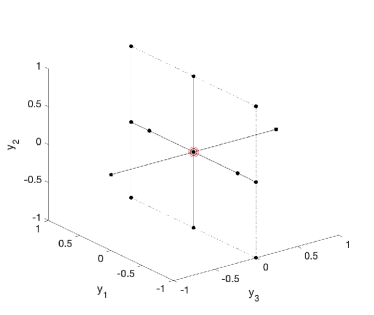
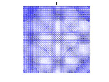
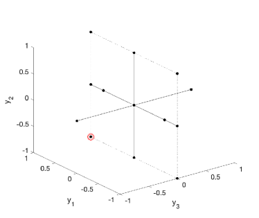
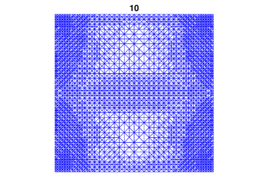
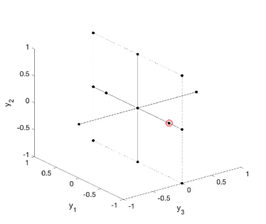
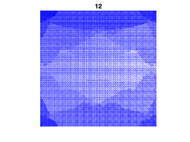
Figure 1. Selected collocation point (left) and corresponding spatial mesh (right) that is generated by the multilevel adaptive strategy for test case I.

A reference solution to this problem with $M$ set to 4 is illustrated in Fig. 1 in [5]. This solution was generated by running the single-level algorithm with the $\tt{errortolerance}$ set to 6e-3, starting from a uniform initial mesh with 81 vertices and a sparse grid consisting of a single collocation point. The threshold parameter $\vartheta$ was set to 1, the marking parameters $\theta_{\mathbb{X}}$ and $\theta_{\mathcal{Y}}$ were set to 0.3. The error tolerance was satisfied after 25 iterations comprising 20 spatial refinement steps and 5 parametric refinement steps. There were 13 Clenshaw–Curtis sparse grid collocation points when the iteration terminated. These points are visualized in Fig. 1. The associated sparse grid indices are listed in Table 1 in [5]. The final spatial mesh is shown in Fig. 2 in [5]. The number of vertices in this mesh is 16,473 so the total number of degrees of freedom when the error tolerance was satisfied when running the single-level algorithm was 214,149.

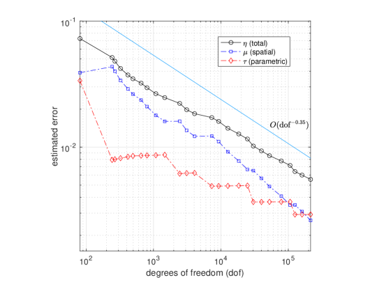
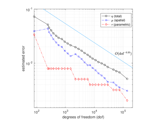
Figure 2. Evolution of the single-level error estimates (top) and the multilevel error estimates (bottom) for test case I with error tolerance set to 6e-3.

The first test of the multilevel algorithm is to repeat the above experiment; that is, starting from the same point with identical marking parameters $\vartheta=1$, $\theta_{\mathbb{X}}=\theta_{\mathcal{Y}}=0.3$ (we also set the marking parameter $\theta$ in Algorithm 3 to the same value as $\theta_{\mathbb{X}}$ in all our experiments). Specifying the same error tolerance 6e-3 led to the the same 13 collocation points being activated, in this case after 26 rather than 25 iterations. A comparison of the single-level and multilevel error estimates is given in Fig. 2. While the final number of degrees of freedom is reduced from 214,149 to 137,943 in the multilevel case, the rate of convergence is still far from optimal (close to $O({\rm dof}^{-1/3})$).

The degree of refinement of the final meshes associated with some specific collocation points is illustrated in Fig. 1. The two finest meshes had over 32,000 vertices and are associated with the pair of collocation points that are activated by the sparse grid index 3 1 1 1 that is introduced at the final iteration (one of these collocation points and the corresponding mesh are shown in the bottom plot). The two coarsest meshes had close to 3,600 vertices; one of these is shown in the middle plot. The mesh that is associated with the mean field $a_{0}=1$ has 11,157 vertices and is shown in the topmost plot. As might be anticipated, the level of refinement of this mesh is less than that of the final mesh that is generated by the single-level strategy.

It is worth pointing out that in our extensive experimentations with other choices of marking parameters the adaptive multilevel SC-FEM algorithm did not exhibit a faster convergence rate compared to that of the single-level algorithm for the respective choice of marking parameters. This is in contrast to SGFEM, where multilevel adaptivity always results in a faster convergence rate than that of the single-level counterpart for problems with affine-parametric coefficients including the test case considered here; see [8, 6, 3, 2]. Furthermore, for this class of problems, the analysis in [2] has shown that, under an appropriate saturation assumption, the adaptive multilevel SGFEM algorithm driven by a two-level a posteriori error estimator and employing a Dörfler-type marking on the joint set of spatial and parametric indicators yields optimal convergence rates with respect to the number of degrees of freedom in the underlying multilevel approximation space.

4.2. Test case II: nonaffine coefficient data

In this case, we set $f=1$ and look to solve the first model problem on the L-shaped domain $D=(-1,1)^{2}\backslash(-1,0]^{2}$ with coefficient $a(x,\mathbf{y})=\exp(h(x,\mathbf{y}))$, where the exponent field $h(x,\mathbf{y})$ has affine dependence on parameters $y_{m}$ that are images of uniformly distributed independent mean-zero random variables,

$$h(x,\mathbf{y})=h_{0}(x)+\sum_{m=1}^{{\color[rgb]{0,0,0}4}}h_{m}(x)\,y_{m},\quad x\in D,\ \mathbf{y}\in\Gamma.$$ (16)

We further specify $h_{0}(x)\,{=}\,1$ and $h_{m}(x)=\sqrt{\lambda_{m}}\varphi_{m}(x)$ ($m=1,\ldots,{\color[rgb]{0,0,0}4}$). Here $\{(\lambda_{m},\varphi_{m})\}_{m=1}^{\infty}$ are the eigenpairs of the integral operator $\int_{{\color[rgb]{0,0,0}D\cup(-1,0]^{2}}}\hbox{\rm Cov}[{\color[rgb]{0,0,0}h}](x,x^{\prime})\varphi(x^{\prime})\,\hbox{d}x^{\prime}$ with a synthetic covariance function given by

$$\hbox{\rm Cov}[{\color[rgb]{0,0,0}h}](x,x^{\prime})=\sigma^{2}\exp\left(-|x_{1}-x_{1}^{\prime}|-|x_{2}-x_{2}^{\prime}|\right).$$ (17)

The standard deviation $\sigma$ is set to 1.5 in order to mirror the most challenging test case in §5.2 of [5]. The convergence of the multilevel adaptive algorithm, starting with one collocation point and with the initial grid shown in Fig. 7 of [5]  is compared with the single-level result in Fig. 3. The multilevel algorithm is again run using the marking parameters $\theta_{\mathbb{X}}=\theta_{\mathcal{Y}}=0.3$ specified in [5] and the same error tolerance, that is 6e-3.

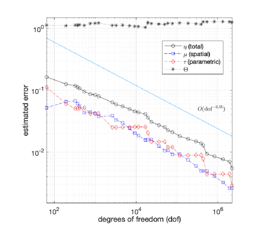
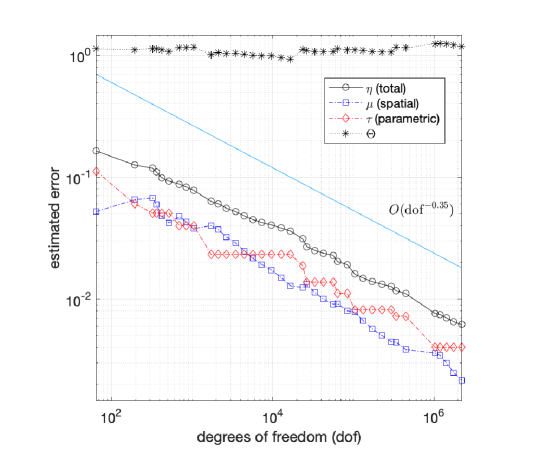
Figure 3. Evolution of the single-level error estimates (top) and the multilevel error estimates (bottom) for test case II with error tolerance set to 6e-3.

These results reinforce the view that performance gains from the multilevel strategy are difficult to realize. While the number of active collocation points is smaller in the multilevel case (51 vs 57; the sparse grid index 2 1 2 2 added at the final single-level iteration is not included), the total number of degrees of freedom when the tolerance is reached is almost identical (2,212,393 vs 2,190,847). The issue here is that meshes associated with mixed indices with multiple active dimensions have multiple features that require resolution. Thus, the most refined grid associated with the index that is introduced in the final parametric enhancement has 428,972 vertices. This is significantly more refined than the final grid that is generated in the single-level implementation, which had 37,133 vertices. This fact, together with the increase in the number of adaptive steps taken (37 vs 31) means that the overall computation time is significantly increased when the multilevel strategy is adopted.

The plots in Fig. 3 also show that the use of the coarsest-mesh approximations for computing the parametric error estimates $\tau_{\ell}$ in (12) does not affect the overall effectivity of the error estimation in the multilevel algorithm. Indeed, in the single-level algorithm (where parametric error estimates employ the (single) refined mesh underlying the current SC-FEM solution $u_{\ell}^{\rm SC}$), the effectivity indices $\Theta_{\ell}$ computed at each iteration range between 1.047 and 1.296, whereas for the multilevel algorithm they stay between 0.930 and 1.257.

4.3. Test case III: one peak problem

We are looking to solve the Poisson equation $-\nabla^{2}u=f$ in a unit square domain $D=(-4,4)\times(-4,4)$ with Dirichlet boundary data $u=g$. The source term $f$ and boundary data are uncertain and are parameterized by $\mathbf{y}=(y_{1},y_{2})$, representing the image of a pair of independent random variables with $y_{j}\sim{U}[-1,1]$. In the vanilla case discussed in [11], the same test problem is posed on the unit domain $I=(-1,1)\times(-1,1)$ with $y_{j}\sim{U}[-1/4,1/4]$. The source term $f$ and the boundary data $g$ are chosen so that the problem has a specific pathwise solution given by

$$u(x,\mathbf{y}) =\exp(-\beta\{(x_{1}-y_{1})^{2}+(x_{2}-y_{2})^{2}\}),$$ (18)

where a scaling factor $\beta=50$ is chosen to generate a highly localized Gaussian profile centered at the uncertain spatial location $(y_{1},y_{2})$.

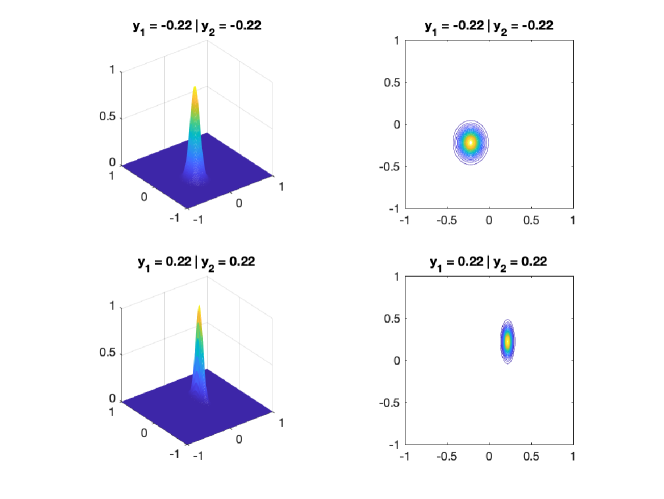
Figure 4. One peak problem solutions on the unit domain: $\alpha=1.54$ (top), $\alpha=9.46$ (bottom).

In the paper [12], the one peak test problem defined on the unit domain is made anisotropic by scaling the solution in the first coordinate direction by a linear function $\alpha(y_{1})=18y_{1}+11/2$ so that $\alpha$ takes values in the interval $[{\color[rgb]{0,0,0}1},10]$. The corresponding pathwise solution is then given by

$$u(x,\mathbf{y}) =\exp(-{\color[rgb]{0,0,0}50}\{\alpha(y_{1})(x_{1}-y_{1})^{2}+(x_{2}-y_{2})^{2}\}).$$ (19)

The solution (19) is generated by specifying an uncertain forcing function

$$f(x,\mathbf{y}) =d(x_{1},x_{2},y_{1},y_{2})\cdot\exp(-\beta\{\alpha(y_{1})(x_{1}-y_{1})^{2}+(x_{2}-y_{2})^{2}\})$$ (20a)

with

$$d(x_{1},x_{2},y_{1},y_{2}) =-4\beta^{2}\left\{\alpha^{2}(y_{1})(x_{1}-y_{1})^{2}+(x_{2}-y_{2})^{2}\right\}+2\beta(\alpha(y_{1})+1).$$ (20b)

Realisations of the reference solution (19) are shown at two distinct sample points in Fig. 4. The anisotropy introduced by the scaling with $\alpha$ is a clear feature.

Our specific goal is to compute the following quantity of interest (QoI)

$$\mathbb{E}\left[\phi_{{\color[rgb]{0,0,0}I}}(u)\right] =\int_{{\color[rgb]{0,0,0}\left[-\frac{1}{4},\frac{1}{4}\right]^{2}}}\int_{I}u^{2}(x,\mathbf{y})\,\mathrm{d}x\,{\color[rgb]{0,0,0}\mathrm{d}\pi(\mathbf{y})},$$ (21)

where $\phi_{{\color[rgb]{0,0,0}I}}(u)=\int_{I}u^{2}(x,\cdot)\,\mathrm{d}x$. The choice $\beta=50$ is then helpful for two reasons:

• The Dirichlet boundary condition ($u$ satisfying (19) on $\partial I$) may be replaced without significant loss of accuracy by the numerical approximation $u_{\bullet\mathbf{z}}=0$ on $\partial I$.

• A reference value (accurate to more than 10 digits)

  $$\mathbb{E}\left[\phi_{{\color[rgb]{0,0,0}I}}(u)\right]\approx Q:={1\over 9}\cdot(\sqrt{10}-1)\cdot{\pi\over\beta}=0.015095545\ldots$$ (22)

  may be readily computed; see [12, Appendix] for details.

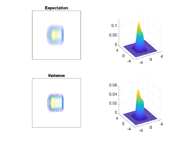
Figure 5. Reference solution for test case III.

We compute estimates of the QoI by solving the problem (1b) using the coordinate transformations $x_{j}\leftarrow 4x_{j}$ and $y_{j}\leftarrow 4y_{j}$ ($j=1,2$). In this case, the pathwise solution on the scaled domain $D\times\Gamma$ is given by (19) by specifying $\beta=50/16$ and $\alpha(y_{1})=(9y_{1}+11)/2$. Moreover, the QoI in (21) (and its reference value given in (22)) can be estimated within Algorithm 1 by computing the following quantity:

$${\color[rgb]{0,0,0}\frac{1}{16}}\,\mathbb{E}\left[\phi_{{\color[rgb]{0,0,0}D}}({\color[rgb]{0,0,0}u_{\ell}^{\rm SC}})\right] ={1\over 16}\,\int_{\Gamma}\int_{D}{\color[rgb]{0,0,0}\big{(}u_{\ell}^{\rm SC}(x,\mathbf{y})\big{)}^{2}}\,\mathrm{d}x\,{\color[rgb]{0,0,0}\mathrm{d}\pi(\mathbf{y})}.$$

A reference solution to the scaled problem is shown in Fig. 5.

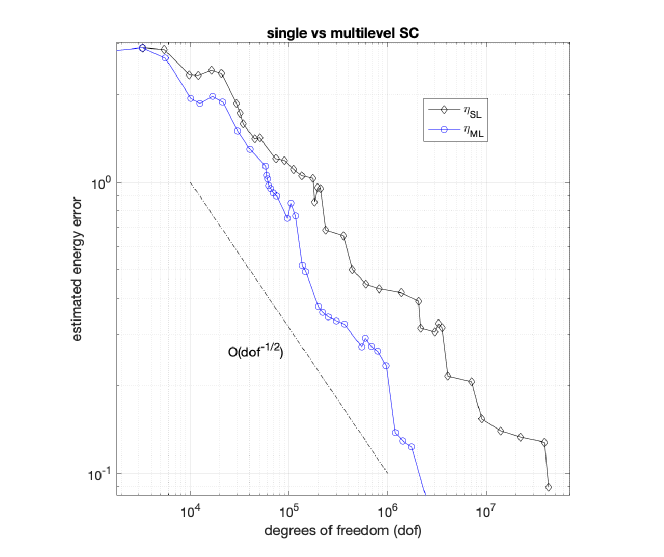
Figure 6. Evolution of the single-level and multilevel error estimates for the one peak test problem with error tolerance set to 1e-1.

A comparison of the single-level and multilevel SC-FEM algorithms when applied to the one peak test problem is given by the evolution of error estimates in Fig. 6. The single-level algorithm reached the tolerance in 37 steps with 169 active collocation points and the final approximation had 42,961,659 degrees of freedom. The multilevel algorithm proved to be much more efficient. The same tolerance was reached in 34 steps with 153 collocation points in the final approximation space. Crucially, each collocation point is associated with a mesh that is locally refined in the vicinity of the respective point in $D$ (as illustrated in Fig. 7). In contrast, the final mesh generated by the adaptive single-level SC-FEM has refinement everywhere in a larger region corresponding to the union of supports of all sampled solutions. When the error tolerance was reached, both algorithms gave estimates of the QoI that agreed with the reference value to five decimal places (0.015092 for the single-level case vs 0.015087 for the multilevel case).

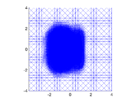
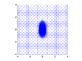
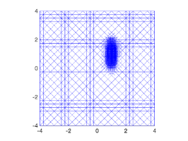
Figure 7. Single-level mesh (left) and meshes associated with the central collocation point (middle) and top right corner point (right) when the tolerance is reached for test case III.

The upshot of the effective use of tailored refinement is an order of magnitude decrease in the overall computation time. The total number of degrees of freedom in the multilevel case was 2,620,343—a factor of 16 reduction overall. Looking at the associated rates of convergence we see that the optimal rate $O({\rm dof}^{-1/2})$ is recovered in the multilevel case. We anticipate that similar performance gains will be realized whenever a problem has local features that can be effectively resolved using sample-dependent meshes.

We have also solved the one peak test problem using an efficient adaptive stochastic Galerkin approximation strategy. While the linear algebra associated with the Galerkin formulation is decoupled in this case, the computational overhead of evaluating the right-hand side vector is a significant limiting factor in terms of the relative efficiency. The overall CPU time taken to compute 4 digits in the QoI using adaptive stochastic Galerkin FEM is comparable to the CPU time taken to compute 5 digits using the multilevel SC-FEM strategy.

5. Conclusions

Adaptive methods hold the key to efficient approximation of solutions to linear elliptic partial differential equations with random data. The numerical results presented in this series of two papers demonstrate the effectiveness and the robustness of our novel SC-FEM error estimation strategy, as well as the utility of the error indicators guiding the adaptive refinement process. Our results also suggest that optimal rates of convergence are more difficult to achieve in a sparse grid collocation framework than in a multilevel stochastic Galerkin framework. It is demonstrated herein that the overhead of generating specially tailored sample-dependent meshes can be worthwhile and optimal convergence rates can be recovered when the solutions to the sampled problems have local features in space. The single-level strategy discussed in part I of this work is, however, likely to be more efficient (certainly in terms of overall CPU time) when a single adaptively refined grid can adequately resolve spatial features associated with solutions to a range of individually sampled problems.

References

- [1] I. Babuška, F. Nobile, and R. Tempone, A stochastic collocation method for elliptic partial differential equations with random input data, SIAM J. Numer. Anal., 45 (2007), pp. 1005–1034.
- [2] A. Bespalov, D. Praetorius, and M. Ruggeri, Convergence and rate optimality of adaptive multilevel stochastic Galerkin FEM, IMA J. Numer. Anal., (2021). (appeared online; https://doi.org/10.1093/imanum/drab036).
- [3] , Two-level a posteriori error estimation for adaptive multilevel stochastic Galerkin FEM, SIAM/ASA J. Uncertain. Quantif., 9 (2021), pp. 1184–1216.
- [4] A. Bespalov and D. Silvester, Efficient adaptive stochastic Galerkin methods for parametric operator equations, SIAM J. Sci. Comput., 38 (2016), pp. A2118–A2140.
- [5] A. Bespalov, D. Silvester, and F. Xu, Error estimation and adaptivity for stochastic collocation finite elements part I: single-level approximation. Preprint, arXiv:2109.07320 [math.NA], 2021.
- [6] A. J. Crowder, C. E. Powell, and A. Bespalov, Efficient adaptive multilevel stochastic Galerkin approximation using implicit a posteriori error estimation, SIAM J. Sci. Comput., 41 (2019), pp. A1681–A1705.
- [7] M. Eigel, O. Ernst, B. Sprungk, and L. Tamellini, On the convergence of adaptive stochastic collocation for elliptic partial differential equations with affine diffusion. Preprint, arXiv:2008.07186 [math.NA], 2020.
- [8] M. Eigel, C. J. Gittelson, C. Schwab, and E. Zander, Adaptive stochastic Galerkin FEM, Comput. Methods Appl. Mech. Engrg., 270 (2014), pp. 247–269.
- [9] M. Feischl and A. Scaglioni, Convergence of adaptive stochastic collocation with finite elements, Comput. Math. Appl., 98 (2021), pp. 139–156.
- [10] D. Guignard and F. Nobile, A posteriori error estimation for the stochastic collocation finite element method, SIAM J. Numer. Anal., 56 (2018), pp. 3121–3143.
- [11] R. Kornhuber and E. Youett, Adaptive multilevel Monte Carlo methods for stochastic variational inequalities, SIAM J. Numer. Anal., 56 (2018), pp. 1987–2007.
- [12] J. Lang, R. Scheichl, and D. Silvester, A fully adaptive multilevel stochastic collocation strategy for solving elliptic PDEs with random data, J. Comput. Phys., 419 (2020), pp. 109692, 17.
- [13] A. L. Teckentrup, P. Jantsch, C. Webster, and M. Gunzburger, A multilevel stochastic collocation method for partial differential equations with random input data, SIAM/ASA J. Uncertain., 3 (2015), pp. 1046–1074.