BADDr: Bayes-Adaptive Deep Dropout RL for POMDPs

Abstract.

While reinforcement learning (RL) has made great advances in scalability, exploration and partial observability are still active research topics. In contrast, Bayesian RL (BRL) provides a principled answer to both state estimation and the exploration-exploitation trade-off, but struggles to scale. To tackle this challenge, BRL frameworks with various prior assumptions have been proposed, with varied success. This work presents a representation-agnostic formulation of BRL under partially observability, unifying the previous models under one theoretical umbrella. To demonstrate its practical significance we also propose a novel derivation, Bayes-Adaptive Deep Dropout rl (BADDr), based on dropout networks. Under this parameterization, in contrast to previous work, the belief over the state and dynamics is a more scalable inference problem. We choose actions through Monte-Carlo tree search and empirically show that our method is competitive with state-of-the-art BRL methods on small domains while being able to solve much larger ones.

ACM Reference Format:
Sammie Katt, Hai Nguyen, Frans A. Oliehoek, and Christopher Amato. 2022. BADDr: Bayes-Adaptive Deep Dropout RL for POMDPs. In Proc. of the 21st International Conference on Autonomous Agents and Multiagent Systems (AAMAS 2022), Online, May 9–13, 2022, IFAAMAS, 9 pages.

1. Introduction: Bayesian RL

Reinforcement learning Sutton and Barto (1998) with observable states has seen impressive advances with the breakthrough of deep RL Mnih et al. (2013); Silver et al. (2016); Hasselt et al. (2016). These methods have been extended to partially observable environments Kaelbling et al. (1998) with recurrent layers Hausknecht and Stone (2015); Wierstra et al. (2007) and much attention has been paid to encode history into these models Karkus et al. (2018); Jonschkowski et al. (2018); Igl et al. (2018); Ma et al. (2020).

Although successful for some domains, this progress has largely been driven by function approximation and fundamental questions are still left unanswered. The trade-off between between exploiting current knowledge and exploring for new information, is one such example Bellemare et al. (2016); Azizzadenesheli et al. (2018); Osband et al. (2018). Another is how to encode domain knowledge, often abundantly available and crucial for most real world problems (simulators, experts etc.). Although research is actively trying to solve these issues, applications of RL to a broad range of applications is limited without reliable solutions.

Interestingly, Bayesian RL (BRL) suffers from opposite challenges. BRL methods explicitly assume priors over, and maintain uncertainty estimates of, variables of interest. As a result, BRL is well-equipped to exploit expert knowledge and can intelligently explore to reduce uncertainty over (only the) important unknowns. Unfortunately these properties come at a price, and BRL is traditionally known to struggle scaling to larger problems. For example, the BA-POMDP Ross et al. (2011); Katt et al. (2017) is a state-of-the-art Bayesian solution for RL in partially observable environments, but is limited to tabular domains. While factored models can help Katt et al. (2019), such representations are not appropriate or may still suffer from scalability issues.

This work combines the principled Bayesian perspective with the scalability of neural networks. We first generalize previous work Ross et al. (2011); Ghavamzadeh et al. (2016); Katt et al. (2019) with a Bayesian partial observable RL formulation without prior assumptions on parametrization. In particular, we define the general BA-POMDP (GBA-POMDP) which, given a (parameterized) prior and update function, converts the BRL problem into a POMDP with known dynamics. We show that, when the update function satisfies an intuitive criterion, this conversion is lossless and a planning solution to the GBA-POMDP results in optimal behavior for the original learning problem with respect to the prior. To show its practical significance we derive Bayes-adaptive deep dropout RL (BADDr) from the GBA-POMDP. BADDr utilizes dropout networks as approximate Bayesian estimates Gal and Ghahramani (2016), allowing for an expressive and scalable approach. Additionally, the prior is straightforward to generate and requires fewer assumptions than previous BRL methods. The resulting planning problem is solved with new MCTS Browne et al. (2012); Silver and Veness (2010) and particle filtering Thrun (2000) algorithms.

We demonstrate BADDr is not only competitive with state-of-the-art BRL methods in traditional domains, but solves domains that are infeasible for said baselines. We also demonstrate the sample efficiency of BRL in a comparison with the (non-Bayesian) DPFRL Ma et al. (2020) and provide ablation studies and belief analysis.

2. Preliminaries

Partially observable MDPs

Sequential decision making with hidden state is typically modeled as a partially observable Markov decision process (POMDP) Kaelbling et al. (1998), which is described by the tuple $(\mathbb{S,A,O},\mathcal{D},\mathcal{R},\gamma,K,p_{s_{0}})$. Here $\mathbb{S,A}$ and $\mathbb{O}$ are respectively the discrete state, action and observation space. $K\in\mathbb{N}$ is the horizon (length) of the problem, while $\gamma\in[0,1]$ is the discount factor. The dynamics are described by $\mathcal{D}$: $(\mathbb{S}\times\mathbb{A})\rightarrow\Delta(\mathbb{S}\times\mathbb{O})$, which in practice separates into a transition and observation model. The reward function $\mathcal{R}$: $(\mathbb{S}\times\mathbb{A}\times\mathbb{S})\rightarrow\mathbb{R}$ maps transitions to a reward. Lastly, the prior $p_{s_{0}}\in\Delta\mathbb{S}$ dictates the distribution over the initial state.

At every time step $t$ the agent takes an action $a$ and causes a transition to a new hidden state $s^{\prime}$, which results in some observation $o$ and reward $r$. We assume the objective is to maximize the discounted accumulated reward $\sum_{t}\gamma^{t}r_{t}$. To do so, the agent considers the observable history $h_{t}=(\and,\@vec{o}_{t})=(a_{0},o_{1},a_{1},\dots a_{t-1},o_{t})$. Because this grows indefinitely, it is instead common to use the belief $b\in\mathbb{B}$: $\Delta\mathbb{S}$, a distribution over the current state and a sufficient statistic Kaelbling et al. (1998). The belief update, $\tau$: $(\mathbb{B}\times\mathbb{A}\times\mathbb{O})\rightarrow\mathbb{B}$, gives the new belief after an action and observation, and follows the Bayes’ rule:

$$b^{\prime}(s^{\prime})=\tau(b,a,o)(s^{\prime})\propto\sum_{s}\mathcal{D}(s^{\prime},o|s,a)b(s)$$ (1)

A policy then maps beliefs to action probabilities $\pi$: $\mathbb{B}\rightarrow\Delta\mathbb{A}$.

In this work we will be concerned with solving large POMDPs in which exact belief updates and planning are no longer feasible. For efficient belief tracking we use particle filters Thrun (2000), which approximate the belief with a collection of ‘particles’ (in this case states). For action selection we turn to online planners, since they can spend resources on only the beliefs that are relevant. In particular, this work builds on POMCP Silver and Veness (2010), an extension of Monte-Carlo tree search (MCTS) Kocsis and Szepesvári (2006); Browne et al. (2012) to POMDPs, that is compatible with particle filtering. More details follow in the method section (section 4.2).

Dropout neural networks

Dropout Li and Gal (2017); Gal and Ghahramani (2016); Srivastava et al. (2014); Hinton et al. (2012) is a stochastic regularization technique that samples networks by randomly dropping nodes (setting their output to zero). A nice property is that it can be interpreted as performing approximate Bayesian inference. Specifically Gal and Ghahramani (Gal and Ghahramani, 2016) show that applying dropout to a (fully connected) layer $i$ means that its $K_{i}$ inputs $j$ are active (or dropped) according to Bernoulli variables $z_{i,j}$. This means that a (random) effective weight matrix for that layer randomly drops columns: it can be written as $\tilde{\mathbf{W}}_{i}=\mathbf{W}_{i}\cdot\textrm{diag}([z_{i,j}]_{j=1}^{K_{i}})$. We define $w$ as the stacking of all such (effective) layer weights, and $\tilde{w}\sim dropout(\cdot|w)$ as the distribution induced by dropout. Gal and Ghahramani show that the training objective of a dropout network minimizes the Kullback-Leibler divergence between $dropout(w)$ and the posterior over weights of a deep Gaussian process (GP Damianou and Lawrence (2013)), a very general powerful model for maintaining distributions over functions. A result of this is a relatively cheap method to compute posterior predictions using Monte-Carlo estimates:

$$p(y|x)\approx\frac{1}{N}\sum_{n=0}^{N}p(y|x;\tilde{w}_{n})$$ (2)

3. Bayesian Partially Observable RL

The strength of Bayesian RL is that it can exploit prior (expert) knowledge in the form of a probabilistic prior to better direct exploration and thus reduce sample complexity. However, to operationalize this idea, previous approaches make limiting assumptions on the form of the prior (such as assuming it is given as a collection of Dirichlet distributions), which limits their scalability.

Here we present the Bayesian perspective of the partially observable RL (PORL) problem without such assumptions. We first formalize precisely what we mean with PORL in section 3.1. Section 3.2 then describes the process of Bayesian belief tracking for PORL in terms of general densities over dynamics. This makes explicit how the belief can be interpreted as a weighted mixture of posteriors given the full history (something which we will exploit in section 4). Subsequently, in section 3.3 we state a parameter update criterion that provides sufficient conditions for a parameterized representation to give an exact solution to the original PORL problem. Finally, section 3.4 then describes how we can cast the PORL problem as a planning problem using arbitrary parameterized distributions in the proposed general BA-POMDP (GBA-POMDP).

The GBA-POMDP naturally generalizes over previous realizations (e.g. Katt et al. (2019)), but also support low-dimensional or hierarchical representations of beliefs. We note that in some cases, such more compact belief representation have been used in experiments Ross et al. (2011) even though they were not captured by the theory presented in the paper. Our paper in that way provides the, thus far still missing, theoretical underpinning for these experiment. Later in section 4 we will show its practical significance, where we derive a neural network based realization that is capable of modeling larger problems than current state-of-the-art Bayesian methods can.

3.1. Bayesian PORL Definitions

Here we formalize the problem of partially observable RL (PORL) and the Bayesian perspective on it. In PORL the goal is to maximize some metric while being uncertain about which POMDP we act in:

Definition 0 (Family of POMDPs).

Given a set of dynamics functions $\mathfrak{D}$, we say that $\mathcal{F}=\left\{(\mathbb{S,A,O},\mathcal{D},\mathcal{R},\gamma,K,p_{s_{0}})\mid\mathcal{D}\in\mathfrak{D}\right\}$ is a family of POMDPs.

Note that we assume that only the dynamics function is unknown. In our formulation, the reward function is assumed to be known (even though that can be generalized, e.g., by absorbing the reward in the state), as well as the representation of hidden states. We assume that the goal is to maximize the expected cumulative (discounted) reward over a finite horizon, but other optimality criteria can be considered.

We now consider Bayesian learning in such families when a prior $p_{\mathcal{D}}$ over the (otherwise unknown) dynamics is available:

Definition 0 (BPORL: Bayesian partial observable RL).

A BPORL model $\mathcal{M}_{\text{BPORL}}=(\mathcal{F},p_{\mathcal{D}})$ is a family of POMDPs $\mathcal{F}$ together with a prior over dynamics functions $p_{\mathcal{D}}\in\Delta\mathfrak{D}$.

3.2. Belief Tracking in Bayesian PORL

Figure 1. Model of the BRL inference problem. The actions $a$ and observations $o$ in gray are observable, which means the policy is dependent on them, while the states $s$ and dynamics $\mathcal{D}$ are hidden. The priors $p_{\mathcal{D}}$ and $p_{s_{0}}$ represent the a-priori knowledge. Time is indicated with subscripts and progresses to the right.

A graphical representation of the BRL inference problem. Describes both POMDP elements such as states, observations and actions, as well as the (unknown) dynamics and the Bayesian priors over it.

Here we first derive the equations that describe belief tracking in a BPORL, not making any assumption on parametrization of these beliefs, but instead assuming arbitrary densities. The data available to the agent is the observable history $h_{t}$, the previous actions and observations, as well as the priors $p_{\mathcal{D}}$ and $p_{s_{0}}$ (fig. 1), which are implicitly assumed throughout and omitted in the equations. The quantity of interest is the belief over the current POMDP state and dynamics $p(\mathcal{D},s_{t}|h_{t})$. We consider how to compute the next belief $p(\mathcal{D},s_{t+1}|h_{t+1})$ from a current $p(\mathcal{D},s_{t}|h_{t})$ given a new action $a_{t}$ and observation $o_{t+1}$. Note the similarities to the POMDP belief update eq. 1 and how it unrolls over time steps.

$$p(\mathcal{D},s_{t+1}|h_{t+1}) \propto\sum_{s_{t}}\mathcal{D}(s_{t+1},o_{t+1}|s_{t},a_{t})p(\mathcal{D},s_{t}|h_{t})$$ (3)

$$(\text{unroll t}) \propto p_{\mathcal{D}}(\mathcal{D})\sum_{\@vec{s}_{t}}p_{s_{0}}(s_{0})\prod_{i=0}^{t}\mathcal{D}(s_{i+1},o_{i+1}|s_{i},a_{i})$$ (4)

This assigns more weights to models that are more probable under the evidence and is fine in general from the Bayesian perspective. Unfortunately, the joint space of models and states is too large to do exact inference on and, in practice, we need to resort to approximations and consider only a limited number of models. The “true” model $\mathcal{D}$ will typically not be part of the tracked models, and merely updating their weights as in eq. 4 is inadequate: it will lead to degenerate beliefs where most weights approach zero. To address this, we rewrite eq. 3 such that it gives a different perspective, one which updates the models considered by the belief, and this opens the possibility for combinations with machine learning methods. We denote the history including a state sequence $\@vec{s}_{t}$ with $H_{t}=(\@vec{s}_{t},h_{t})=(s_{0},a_{0},s_{1},o_{1}\dots a_{t-1},s_{t},o_{t})$ and apply the chain rule to formulate the belief as a weighted mixture of model posteriors (one for each state sequence $\@vec{s}_{t}$):

$$p(\mathcal{D},s_{t+1}|h_{t+1})=\sum_{\@vec{s}_{t}}\underbrace{p(\@vec{s}_{t+1}|h_{t+1})}_{\text{weight}}\underbrace{p(\mathcal{D}|H_{t+1})}_{\text{component}}$$ (5)

The advantage is that it includes the term $p(\mathcal{D}|H_{t})$ that can be interpreted as a posterior over the model given all the data $H_{t}$. In the supplements we show that this belief can be computed recursively:

$$(\ref{eq:mixture-brl})\propto\sum_{\@vec{s}_{t}}\underbrace{p(\@vec{s}_{t}|h_{t})}_{\text{prior weight}}\underbrace{p(s_{t+1},o_{t+1}|H_{t},a_{t})}_{\text{transition likelihood}}\underbrace{p(\mathcal{D}|H_{t+1})}_{\text{component}}$$ (6)

Here the prior weight $p(\@vec{s}_{t}|h_{t})$ is the weight of one of the components in the belief at the previous time step (eq. 5). The transition likelihood is not trivial and is an expectation over the dynamics:

$$p(s_{t+1},o_{t+1}|H_{t},a_{t})=\int_{\mathcal{D}}p(\mathcal{D}|H_{t})\mathcal{D}(s_{t+1},o_{t+1}|s_{t},a_{t})$$ (7)

Lastly, the component $p(\mathcal{D}|H_{t+1})$ is the posterior over the model given all observable data plus a hypothetical state sequence. This term, and its computation, is explained in the next section.

3.3. Parameterized Representations

The last section described the belief in BPORL as a mixture where each component itself is a distribution over the dynamics (eq. 5). It also provided the corresponding belief update (eq. 6), but omitted the computation of the components. Here we show how a posterior $p(\mathcal{D}|H_{t+1})$ can be derived from a prior component $p(\mathcal{D}|H_{t})$.

In order to make the bridge to practical implementations, we consider the setting where these distributions are parameterized by $\theta\in\Theta$, and denote the induced distribution as $p(\mathcal{D};\theta_{H_{t}})$. Thus we are now interested in a parameter update function that updates parameters given new transitions: $\mathcal{U}$: $(\Theta\times\mathbb{S\times A\times S\times O})\rightarrow\Theta$. This of course raises the question of how such updates can capture the true evaluation of the posterior $p(\mathcal{D}|H_{t})$. To address this, we formalize a parameter update criterion, which can be used to demonstrate that these dynamics are sufficiently captured.

Definition 0 (Parameter update criterion).

We say that the parameter update criterion holds if it is true that, whenever for some $t$ we have that all $H_{t}=(s_{0},a_{0},s_{1},o_{1},a_{1},\dots,a_{t-1},s_{t},o_{t}),a_{t}$ induce the same dynamics as their summary $(\theta_{H_{t}},s_{t})$, for all $s_{t+1},o_{t+1}$

$$p(s_{t+1},o_{t+1}|H_{t},a_{t})=p(s_{t+1},o_{t+1}|\theta_{H_{t}},s_{t},a_{t})$$ (8)

then, for the corresponding transitions, and their induced $H_{t+1}=(H_{t},a_{t},s_{t+1},o_{t+1})$ and $\theta_{H_{t+1}}=\mathcal{U}(\theta_{H_{t}},s_{t},a_{t},s_{t+1},o_{t+1})$, the next stage dynamics are also equal, for all $s_{t+2},o_{t+2}$:

$$p(s_{t+2},o_{t+2}|H_{t+1},s_{t+1},a_{t+1})=p(s_{t+2},o_{t+2}|\theta_{H_{t+1}},s_{t+1},a_{t+1}).$$

From this, we derive:

Lemma 0.

If the parameter update criterion holds, and the initial parameter matches the prior over models:

$$\int_{\mathcal{D}}p_{\mathcal{D}}(\mathcal{D})\mathcal{D}(s_{1},o_{1}|s_{0},a_{0})=p(s_{1},o_{1}|\theta_{0},s_{0},a_{0})$$ (9)

then we have that for all $t,H_{t},a_{t},s_{t+1},o_{t+1}$

$$p(s_{t+1},o_{t+1}|H_{t},a_{t})=p(s_{t+1},o_{t+1}|\theta_{H_{t}},s_{t},a_{t})$$

Thus, if the parameterization $\theta$ can represent the prior over the dynamics $p_{\mathcal{D}}$ and the parameter update criterion holds, then we can correctly represent and update the true posterior distribution.

Proof.

The proof follows directly from induction. Base case for $t=0$, in which case for $H_{0}=(s_{0})$, holds due to the condition eq. 9

$$p(s_{1},o_{1}|\theta_{0},s_{0},a_{0}) \stackrel{{\scriptstyle(\lx@cref{creftype~refnum}{eq:initial-param-matches-prior})}}{{=}}\int_{\mathcal{D}}p(\mathcal{D}|H_{0})\mathcal{D}(s_{1},o_{1}|s_{0},a_{0})$$

$$\stackrel{{\scriptstyle(\lx@cref{creftype~refnum}{eq:weight-update})}}{{=}}p(s_{t+1},o_{t+1}|H_{0},a_{t})$$

At this point we apply the update criterion as our induction hypothesis and conclude that the posteriors are identical for all $H_{t}$. ∎

Hence, an update $\mathcal{U}$ that satisfies the criterion computes (parameterized) posteriors $p(\mathcal{D}|H_{t+1})$ from a prior component $p(\mathcal{D}|H_{t})$.

The parameter update criterion captures for instance the updating of statistics for conjugate distributions, such as Dirichlet-multinomial distributions, but also situations where the uncertainty about the dynamics functions is captured by a low-dimensional statistic or where a more general a hierarchical representation of the dynamics function is appropriate. Approximate inference methods can also be used to construct parametrizations (of which BADDr will be one example) and Monte-Carlo simulation can be used if sufficient compute power is available.

3.4. General BA-POMDP

The previous sections showed how the belief in the BPORL is a mixture of components, parameterized posteriors over the dynamics, and how to compute them. We use this machinery to rewrite the belief update. Specifically, the belief as a mixture of components (one for each state sequence, eq. 5) will be represented with weighted state-parameter tuples $(s,\theta)$, and the update (eq. 6) will be reformulated as transitions between said tuples:

$$p(\theta_{t+1},s_{t+1}|h_{t+1})\propto\sum_{s_{t},\theta_{t}}\underbrace{p(\theta_{t+1},s_{t+1},o_{t+1}|\theta_{t},s_{t},a_{t})}_{\text{tuple transition probability}}\underbrace{p(\theta_{t},s_{t}|h_{t})}_{\text{prior tuple}}$$

where the transition $p(\theta_{t+1},s_{t+1},o_{t+1}|\theta_{t},s_{t},a_{t})$ factorizes into

$$\underbrace{p(\theta_{t+1}|\theta_{t},s_{t},a_{t},s_{t+1},o_{t+1})}_{\text{parameter update}}\underbrace{p(s_{t+1},o_{t+1}|\theta_{t},s_{t},a_{t})}_{\text{transition likelihood of\leavevmode\nobreak\ \lx@cref{creftype~refnum}{eq:brl-recursive}}}$$

where the parameter update is deterministic and reduces to the indicator function that returns $1$ iff $\theta_{t+1}$ equals the result of $\mathcal{U}$:

$$p(\theta_{t+1}|\theta_{t},s_{t},a_{t},s_{t+1},o_{t+1})=\mathbb{I}(\theta_{t+1},\mathcal{U}(\theta_{t},s_{t},a_{t},s_{t+1},o_{t+1}))$$

The last mental step interprets the tuples as belief/augmented POMDP states, and the equations above as POMDP dynamics, which finally leads to the formulation of the General BA-POMDP:

Definition 0 (General BA-POMDP).

Given a prior $\theta_{0}$, and a parameter update function $\mathcal{U}$, then the general BA-POMDP is a POMDP: $\mathcal{M}_{\text{GBA-POMDP}}(\theta_{0},\mathcal{U})=(\mathbb{\bar{S},A,O},\mathcal{\bar{D},\bar{R}},\gamma,K,p_{\bar{s}_{0}})$ with augmented state space $\bar{S}=(S\times\Theta)$ and prior $p_{\bar{s}_{0}}=(p_{s_{0}},\theta_{0})$. $\mathcal{\bar{R}}$ applies the POMDP reward model $\bar{R}(\bar{s},a,\bar{s^{\prime}})=R(s,a,s)$. Lastly, the update function $\mathcal{U}$ determines the augmented dynamics model $\mathcal{\bar{D}}$:

$$\mathcal{\bar{\mathcal{D}}}(\theta^{\prime},s^{\prime},o|s,\theta,a) \triangleq p(\theta^{\prime}|\theta,s,a,s^{\prime},o)p(s^{\prime},o|\theta,s,a)$$ (10)

$$=\mathbb{I}(\theta^{\prime},\mathcal{U}(\theta,s,a,s^{\prime},o))p(s^{\prime},o|\theta,s,a)$$ (11)

As long as the conditions of section 3.3 hold, the GBA-POMDPs is a representation of a Bayesian PORL problem. Specifically, any BPORL and its GBA-POMDP can be losslessly converted to identical ‘history MDPs’ — we will call them $\mathcal{M}_{\text{BPORL}}^{\text{Hist-MDP}}$ and $\mathcal{M}_{\text{GBA-POMDP}}^{\text{Hist-MDP}}$ — in which the states correspond to action-observation histories $h_{t}$.

Theorem 1.

Given the POMDP $\mathcal{M}_{\text{GBA-POMDP}}=(\theta_{0},\mathcal{U})$ of a Bayesian PORL problem $\mathcal{M}_{\text{BPORL}}=(\mathcal{F},p_{\mathcal{D}})$ and that the parameter update criterion (section 3.3, specifically eqs. 8 and 9) hold, then $\mathcal{M}_{\text{GBA-POMDP}}^{Hist-MDP}=\mathcal{M}_{\text{BPORL}}^{Hist-MDP}$.

Proof.

The basic idea is that we can simply show that due to the matching dynamics of eq. 8, both the rewards $R(h,a)$, as well as transition probabilities $T(h^{\prime}|h,a)$ are identical in the two models. Full proof is given in the supplement. ∎

The upshot of this is that the GBA-POMDP represents the BPORL problem exactly, meaning that optimal solutions are preserved. In this way, it facilitates different, potentially more compact, parametrizations of BPORL problems without necessarily compromising the solution quality. Additionally, like its predecessors, it casts the learning problem as a planning problem, opening up the door of the vast body of POMDP solution methods. This also means that a solution to the GBA-POMDP is a principled answer to the exploration-exploitation trade-off which leads to optimal behavior (which respect to the prior). Lastly, because, unlike its predecessors, it places no assumptions on the prior, it opens the door to a variety of different machine learning methods, as we will see in section 4.

Example realization: tabular-Dirichlet

The BA-POMDP Ross et al. (2011) is the realization of the GBA-POMDP when choosing the prior parameterization $\theta_{0}$ to be the set of Dirichlets. The Dirichlet is the conjugate prior to the categorical distribution and comes with a natural closed-form parameter update: $\mathcal{U}$ in BA-POMDP increments the parameter (‘count’) associated with the transition $(s,a,s^{\prime},o)$.

4. Bayes-Adaptive Deep Dropout RL

The GBA-POMDP is a template for deriving effective BPORL algorithms, but it requires specifying the prior representation and parameter update function. Here we demonstrate how this perspective can lead to tangible benefits by deriving BADDr (Bayes-Adaptive Deep Dropout Reinforcement learning), a GBA-POMDP instantiation based on neural networks. BADDr combines the principled nature of the GBA-POMDP with the scalability of neural networks and Bayesian interpretation of dropout. While BADDr introduces some approximations, our empirical evaluation demonstrates scalability compared to existing BA-POMDP variants and sample efficiency relative to non-Bayes scalable methods.

Here we present BADDr as a (GBA-) POMDP, then section 4.2 describes the resulting solution method.

4.1. BADDr: GBA-POMDP using Dropout

Any GBA-POMDP is defined by its prior and update function. This section defines BADDr’s parameterization, dropout networks $w_{0}$, and the parameter update function $\mathcal{U}$, which further trains these dropout networks, and conclude with the formal definition.

BADDr (prior) parameterization

We represent the dynamics prior with a transition and observation model. The transition model is a neural network parameterized by $w_{\mathcal{T}}$ that maps states and actions into a distribution over next states $f_{w_{\mathcal{T}}}$: $(\mathbb{S}\times\mathbb{A})\rightarrow\Delta\mathbb{S}$, and similarly another network $w_{\mathbb{O}}$ maps actions and next states into a distribution over observations $f_{w_{\mathbb{O}}}$: $(\mathbb{S}\times\mathbb{A}\times\mathbb{S})\rightarrow\Delta\mathbb{O}$. For each state (observation) feature $n$ we predict the probability of its values using softmax. In other words, we have an output (logit) $y_{nm}$ for each value $m$ that feature $n$ can take. Both networks together $w=(w_{\mathcal{T}},w_{\mathbb{O}})$ describe the dynamics. As discussed in section 2, we interpret dropout as an approximation of a posterior (recall eq. 2):

$$p(s^{\prime},o|w,s,a)\approx\frac{1}{N}\sum_{n=0}^{N}p(s^{\prime},o|\tilde{w}_{n},s,a)\text{; }\tilde{w}_{n}\sim dropout(\cdot|w)$$ (12)

BADDr parameter update

We adopt the perspective of training with dropout as approximate Bayesian inference (section 2):

$$p(s_{t+1},o_{t+1}|H_{t},a_{t})\approx p(s_{t+1},o_{t+1}|w_{H_{t}},s_{t},a_{t}).$$ (13)

This raises the question of what the parameter update function should look like: assuming $w_{H_{t}}$ captures the posterior over the dynamics given data $H_{t}$, what operation produces the appropriate next weights given a new transition. A natural choice is to train the dropout network until convergence on all the data available ($H_{t}$ plus the new transition), however this is computationally infeasible and unpractical. Instead we argue a reasonable approximation is to perform a single-step gradient descent step on the new data point.

We denote a gradient step on parameters $w$ given data point $(s,a,s^{\prime},o)$ as $\nabla\mathcal{L}(w;(s,a),(s^{\prime},o))$. The loss is defined as the cross-entropy between the predicted and true next state and observation.

$$\mathcal{L}(w;(s,a),(s^{\prime},o)) =-\log p_{(}s^{\prime},o|s,a;w)$$

$$\mathcal{U}(w,s,a,s^{\prime},o) =w+\nabla\mathcal{L}(w;(s,a),(s^{\prime},o))$$ (14)

Given the prior and update function, we can now define:

Definition 0 (BADDr).

BADDr is a realization of GBA-POMDP $\mathcal{M}_{\text{BADDr}}=\mathcal{M}_{\text{GBA-POMDP}}(w_{0},\mathcal{U})$ with dropout neural networks $w_{0}$ as prior parameterization and a single gradient descent step (eq. 14) as parameter update $\mathcal{U}$. The state space of the resulting POMDP is $\bar{\mathbb{S}}:(\mathbb{S}\times W)$, and its dynamics are described as:

$$\mathcal{\bar{\mathcal{D}}}(\theta^{\prime},s^{\prime},o|s,\theta,a)\triangleq\mathbb{I}(\theta^{\prime},\mathcal{U}(\theta,s,a,s^{\prime},o))p(s^{\prime},o|w,s,a)$$ (15)

where $p(s^{\prime},o|w,s,a)$ is computed according to eq. 12

In this way, BADDR is a specific instantiation of the GBA-POMDP framework. In BADDr, the parameter update criterion (eq. 8) does not hold exactly, since dropout networks only approximate Bayesian inference. This means that we have to rely on empirical evaluation to assess the overall performance, which is shown in section 5.

4.2. Online Planning for BADDr

Here we detail how we use an online planning approach to solve the BADDr model. We start with the construction of our initial belief, then describe how the belief is tracked using particle filtering Thrun (2000), and finish with how MCTS is used to select actions.

Constructing the initial prior

The prior $b(\bar{s}_{0})=p_{0}(s,w)$ is the product of the prior over the model and POMDP state, $(p_{w_{0}},p_{s_{0}})$, where $p_{s_{0}}$ is given by the original learning problem (of the POMDP). Weakening the standard assumption in BRL, we do not require a full prior specification, but assume we can sample domain simulators $\mathbb{M}$. We believe it is more common to be able to generate approximate and/or simplified simulators for real world problems than it is to describe (typically assumed) exhaustive priors.

The prior specification hidden in $\mathbb{M}$ is translated into a network ensemble Dietterich (2000) $\{w_{0}\}$ by training each member on a model sampled $\tilde{M}\sim\mathbb{M}$. The training entails supervised learning on $(s,a,s^{\prime},o)$ samples with loss eq. 14, generated by sampling state-action pairs uniformly and simulating next-state-observation results (from $\tilde{M}$). While this leads to an approximation due to the parametric representation, there is no a problem of data scarcity thanks to the possibility of sampling infinite data from the prior. Hence when using infinitely large neural networks, which are universal function approximators, we theoretically could capture the prior exactly.

Finally the initial particles (belief) is constructed by randomly pairing states $s_{0}\sim p_{s_{0}}$ with networks from the ensemble: $\{(w_{0},s_{0})\}^{n}$. The prior belief for subsequent episodes is generated by substituting the POMDP states in the particle filter with initial states sampled from the prior (and hence maintaining the belief over the dynamics).

Belief tracking

Given the initial particle filter and BADDr’s dynamics eq. 15, we use rejection sampling Thrun (2000) to track the belief. In rejection sampling (algorithm 1) the agent samples a particle $(s,w)$ from particle filter and simulates the execution of a given action $a$. The resulting (simulated) new state $(s^{\prime},w^{\prime})$ is added to the new belief only if the (simulated) observation equals the true observation. Otherwise the sample is rejected. This process repeats until the new belief contains some predefined number of particles.

1:  in: $b$, particle filter $(s,w)$

2:  in: $a$, taken action

3:  in: $o$, new observation

4:  in: $n$, desired number of particles in next belief  

5:  $\bar{b}^{\prime}\leftarrow\emptyset$ // next belief, start empty

6:  while $size(\bar{b}^{\prime})<n$ do

7:     $(s,w)\sim\bar{b}$

8:     // propose sample: BADDr dynamics

9:     $\tilde{w}\sim w$ // dropout sample

10:     $(s^{\prime},\tilde{o})\sim p(\cdot|s,a;\tilde{w})$

11:     $w^{\prime}=w+\nabla\mathcal{L}(w,(s_{t},a_{t}),(s_{t+1},o_{t+1}))$

12:     if $\tilde{o}=o$ then

13:        Add $(s^{\prime},w^{\prime})$ to $\bar{b}^{\prime}$ // correct sampled observation

14:     end if// otherwise reject

15:  end while

16:  return $\bar{b}^{\prime}$

Algorithm 1 Rejection sampling

Algorithm 2 Simulate

1:  pin: $s$, POMDP state

2:  pin: $\tilde{w}$ (root-sampled) dynamics; $\tilde{w}\sim w$

3:  pin: $d$, tree depth

4:  pin: $h$, action-observation history  

5:  if $terminal(h)$ or $d$ is max depth then

6:     return 0

7:  end if

8:  $a\leftarrow ucb(h)$ // UCB Auer et al. (2002) using statistics in node $h$

9:  $s^{\prime},o\sim p(\cdot|s,a;\tilde{w})$ // use root sampled model as simulator

10:  $R\leftarrow\mathcal{R}(s,a,s^{\prime})$ // reward function is given

11:  $h^{\prime}\leftarrow(h,a,o)$

12:  if $h^{\prime}\in tree$ then

13:     $r\leftarrow R+\gamma\times simulate((s^{\prime},w),d+1,h^{\prime})$

14:  else

15:     $initiate\_statistics\_for\_node(h^{\prime})$

16:     $r\leftarrow R+\gamma\times rollout((s^{\prime},w),d+1,h^{\prime})$

17:  end if

18:  $N(h,a)\leftarrow N(h,a)+1$ // update statistics

19:  $Q(h,a)\leftarrow\frac{N(h,a)-1}{N(h,a)}Q(h,a)+\frac{1}{N(h,a)}r$

20:  return $r$

Planning

Ultimately we are interested in taking intelligent actions with respect to the belief — both over the state and the dynamics. As done in previous Bayes-adaptive frameworks Katt et al. (2017, 2019), we also utilize a POMCP Silver and Veness (2010) inspired algorithm. POMCP builds a look-ahead tree of action-observation futures to evaluate the expected return of each action. This tree is built incrementally through simulations (algorithm 2), which each start by sampling a state from the belief. Our approach is different from regular POMCP in the dynamics being used during the simulations and is inspired by model root sampling in BA-POMCP Katt et al. (2017): When POMCP samples a state $(s,w)$ from the belief at the start of a simulation, we subsequently sample a model $\tilde{w}\sim dropout(\cdot|w)$. This model is then used throughout the simulation as the dynamics. The computational advantage is two-fold: one, it avoids computing $\mathcal{U}$ eq. 14 (which requires back-propagation) at each simulated step. Two, the models in the belief need not be copied during root sampling because they are never modified (e.g. if simulations were to update $w$, the pair of networks must be copied to leave the belief untouched).

5. Experiments

In our experiments we compare BADDr to both a state-of-the-art non-Bayesian approach and the (factored) BA-POMDP methods. We experiment on smaller well-known PORL domains, as well as scale up to larger problems. Overall our evaluation shows that, one, BADDr is competitive on smaller problems on which current state-of-the-art BRL methods perform well; and two, BADDr scales to problems that previous methods cannot. Furthermore, qualitative analysis show that the agent’s belief converges around the correct model in tiger and that our method outperforms plain re-weighting of models. Lastly, the strength of Bayesian methods is demonstrated in an comparison with a non-Bayes model-based representative.

5.1. Experimental Setup

Baselines

We compare with (F)BA-POMCP Katt et al. (2019) as the state-of-the-art BRL baseline. To ensure a fair comparison we use their prior as the generative process $\mathbb{M}$ to sample POMDPs from when constructing our prior. Additionally, for all domains, the parameters shared among FBA-POMCP and BADDr (number of simulations & particles, the UCB constant, etc.) are the same. We also plot “POMCP”’ on the true models as an upper bound as dotted lines.

We also include discriminative particle filter reinforcement learning (DPFRL Ma et al. (2020)) as a baseline in our experiments. DPFRL is a novel end-to-end deep RL architecture designed specifically for partial observable environments. We used the official implementation and fine-tuned by picking the best performing combination of the number of particles, learning rate and network sizes.

Small domains & their priors

The experiments on the tiger problem Kaelbling et al. (1998) function as a baseline comparison. This problem is well known for being tiny but otherwise highly stochastic and partial observable. The prior here is a single dropout network trained on the expected model of the prior used in (F)BA-POMCP.

In collision avoidance Luo et al. (2019), the largest problem solved with FBA-POMCP Katt et al. (2019), the agent is a plane flying from the right column of a grid to the left. The last column is occupied by a moving single-cell obstacle that is partially observable and must be avoided. This task is challenging in that both the observation and transition model are highly stochastic. Again we employ their prior — uncertainty over the behavior of the obstacle — to train our ensemble.

We designed the road racing problem, a variable-sized POMDP grid model of highway traffic, in which the agent moves between three lanes in an attempt to overtake other cars (one in each lane). The state is described by the distance of each of those cars in their respective lanes and the current occupied lane. During a step the distance of the other cars decrements with some probability. The speed, and thus the probability of a car coming closer, depends on the lane. The initial distance of all cars is 6, and when their position drops to -1, as the agent overtakes them, it resets. The observation is the distance of the car in the agent’s current lane, which also serves as the reward, penalizing the agent for closing in on cars. The prior over the observation model and the agent’s location transitions is correct. The speed that is associated with each lane, however, is unknown. A reasonable prior is to assume no difference, so we set the expected probability of advancing to 0.5 for all lanes.

Large domains & their priors

We run an additional larger experiment of the road racing problem with nine lanes. This significantly increases the size of the problem and, as will be mentioned in the results, makes previous frameworks intractable.

The last and largest domain is gridverse. Here the agent must navigate from one corner of a grid to the goal in the other, while observing only the cells in front (a beam of width 3 leading to up to $96$ observation features). We run this on a grid of up to 32 by 32 cells. In this environment we assume the observation model is given and learn the transition model of the agent’s position and orientation. For our prior we learn on data generated by a simulator with the correct dynamics for “rotations”, but a noisy “forward” action. The challenge for the agent is to correctly infer the distance of this action (and thus its own location) online.

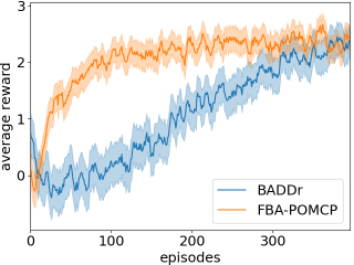
(a) Bayes comparison on tiger.

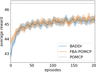
(b) Bayes comparison on road race (3 lanes).

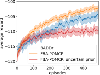
(c) Bayes comparison on collision avoidance.

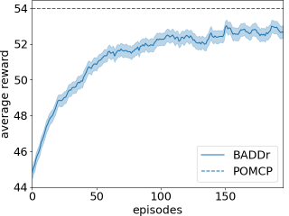
(d) Our work on road race (9 lanes).

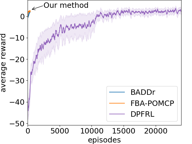
(e) Non-Bayes comparison on tiger.

(f) Non-Bayes comparison on road race (3 & 9).

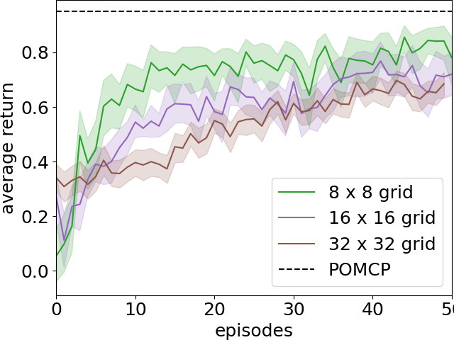
(g) Our work on gridverse.

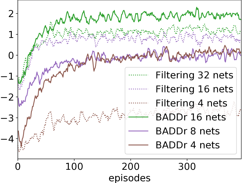
(h) Ablation (no model updates) on tiger.

(i) Belief of tiger observation model.

Figure 2. Our work (blue) is competitive with FBA-POMCP in small problems (a & b), and can scale to larger instances (d & g). Fig. (c) shows that BADDr struggles when prior certainty is crucial. Fig (e & f) compares with DPFRL, where BADDr shows both a better initial performance due to exploiting the prior and better sample efficiency. Dotted lines represent upper bound by running POMCP on the true POMDP. Fig. (h) demonstrates BADDr (solid) requires far fewer models than an ablation method that only re-weights models in its beliefs (dotted). Fig. (i) shows the belief in BADDr on tiger converges to the true value (0.85).

Our work (blue) is competitive with FBA-POMCP in small problems (a & b), and can tackle larger instances (d & g). Fig. (c) shows that BADDr struggles when prior certainty is crucial, but outperforms the baseline otherwise. Fig (e & f) compare our methods with DPFRL. Our methods show both a better initial performance due to exploiting the prior and better sample efficiency. Dotted lines represent upper bound by running POMCP on the true POMDP. Fig. (h) compares BADDr (solid) with an ablation method that only re-weights models in its beliefs (dotted). This ablated approach requires far more initial models which does not scale problems with more variables. Fig. (i) shows the model posterior of BADDr in tiger converges to true value (0.85).

5.2. Bayesian RL Comparison

Small domains

The smaller domains are generally compactly modeled by the (F) BA-POMDP. As a result the baseline BRL methods are near optimal and we cannot expect to do much better. Rather these experiments test whether BADDr is sample efficient even when compared to optimal representations.

Figure 2(a) compares our method with (factored) BA-POMCP on tiger. Unsurprisingly, the tabular representation has a slight advantage initially thanks to the sample efficiency. After twice the amount of data, our method catches up and reaches the same performance. Although Tiger is widely considered a toy problem due to its size, the inference and resulting planning problem are hard: a slight difference in the belief over the model significantly alters the optimal policy. BADDr’s performance here showcases the ability to tackle highly stochastic and partially observable tasks.

We also investigate how well BADDr captures the posterior over the model. Figure 2(i) shows the belief over the probability of hearing the tiger behind the correct door in a particular run. Initially the prior is uncertain and its expectation is incorrect, but over 20 episodes the belief converges to the true value of 0.85.

Figure 2(c) shows BADDr performs nearly as well as FBA-POMCP on the collision avoidance problem. We hypothesize that the representational power of the Dirichlets, in contrast with an ensemble of dropout networks, explains the discrepancy. Specifically, the Dirichlet allow more control over the certainty of the prior: the agent prior over the observation model is confident (high number of counts), and is uncertain over the transition of the obstacle. Admittedly, such a prior is difficult to capture in an ensemble (and thus in BADDr). We test this hypothesis by running FBA-POMCP with an equally uncertain prior, called ‘FBA-POMCP: uncertain prior’. Results show that BADDr performs somewhat in the middle of both. Hence in some occasions the prior representation of BADDr results in diminished performance, but BADDr shows higher potential when both methods are provided similar prior knowledge (as BADDr outperforms ‘FBA-POMCP: uncertain prior’). Note that FBA-POMCP is given the correct (sparse) graphical model, which is a strong assumption in practice that simplifies the learning task.

On the 3-lanes road racing domain (fig. 2(b)) the difference between our work and BA-POMCP is nonexistent. This again confirms that BADDr is competitive with state-of-the-art BRL methods on small problems which these methods are designed for and perform near optimal in. Unlike real applications, these problems are compactly represented by tables and improvements are unlikely.

Larger domains

The advantage of our method becomes obvious in larger problems. In the 9 lanes problem (fig. 2(d)), for instance, even FBA-POMCP has $10^{13}$ entries, is unable represent this compactly, and runs out of memory. But a dropout network of 512 nodes can model the dynamics well enough: despite the increasing size of the problem, the learning curve is similar to the smaller problem (fig. 2(b)) and a similar amount of data is needed to nearly reach the performance of POMCP in the POMDP. This suggests that there is some pattern or generalization that BADDr is exploiting.

Figure 2(g) shows the performance on gridverse on a grid of size 8, 16 and 32. The agent learns to perform nearly as well as if given the true model, indicated by the dotted line (for all 3 sizes), with only a small visible effect of significantly increasing the size of the problem. Note again that for this domain tabular representations are infeasible: a single particle would need to specify up to $10^{7}$ parameters (roughly 40GB of memory for a 64bit system). Bayes networks (FBA-POMDP) is unable to exploit the structure of this domain, which does not show itself through independence between features. However, the dropout networks in the belief of BADDr can generalize to problems otherwise too large to represent.

Ablation study: re-weighting

Section 3.2 claimed that, while technically correct, solely re-weighting models in the belief (eq. 3) leads to belief degeneracy as it relies on a correct (or good) model to be present in the initial belief. This experiments verifies that claim by assessing the performance of plain re-weighting, denoted with ‘filtering’. This is implemented by omitting the parameter update function $\mathcal{U}$ (e.g. SGD step). Figure 2(h) shows that the performance of both filtering (dotted) and BADDr (solid) increases as a function of the number of models in the prior. However, BADDr is significantly more efficient: ‘filtering’ 128 models in the tiger problem performs similarly to BADDr with just 8. Hence, while theoretically possible, it requires too many models to be useful.

Run-time

BADDr is a little slower than FBA-POMCP, since calling (i.e. planning) and training neural networks (i.e belief update) is computationally more expensive than tables. In practice, however, we found this insignificant. In environments where tabular approaches are applicable and fit in memory the difference was at most a small factor. As a result, a single seed/run of any experiment finished within a day on a typical CPU-based Architecture.

5.3. Non-Bayesian RL Comparison

We also ran DPFRL on all domains to investigate the differences between Bayesian and non-Bayesian approaches. Results on tiger (fig. 2(e)) and both road race instances (fig. 2(f)) have been picked out as representative, but other results looked similar and have been included in the appendix. Note the performance of the Bayesian methods are identical to previous plots; only the x-axis is different.

While the eventual performance is similar, the difference in learning speed is immediately obvious. Where the BRL methods learn within tens to hundreds of episodes, DPFRL requires up to tens of thousands — a direct consequence of the sample-efficiency and exploration provided by the Bayesian perspective. In general we found when measuring the number of episodes necessary to reach similar performance, that BADDr was at least 40x (and up to 1200x) more sample efficient than DPFRL.

Another advantage of BRL is the exploitation of a prior, which is visualized by the discrepancy in the initial performance. In the tiger domain DPFRL starts from scratch with a return of ${-}40$ by randomly opening doors. In real applications with real consequences, this can be a huge problem and the ability to encode domain knowledge is crucial. Random behavior is less problematic in the road race domain, yet also there it takes DPFRL thousands of episodes (of many time steps) to reach the performance BADDr has at the start.

6. Related Work

Bayesian RL for discrete POMDPs typically adopts the Dirichlet prior approach taken in the BA-POMDP Ross et al. (2011); Ghavamzadeh et al. (2016). For instance, before generalized to unknown structures with the FBA-POMDP Katt et al. (2019), prior work represented the model posterior as Dirichlets over Bayes network parameters Poupart and Vlassis (2008). Other work circumvents the need for mixtures to represent the posterior by assuming access to an oracle to provide access to the underlying state Jaulmes et al. (2005, 2007). By exploiting this information, they approximate the belief with a MAP estimate of the counts. A notable exception to this line of work is the iPOMDP Doshi-Velez (2009). This work is more general in that knowledge of the state space is not assumed a-priori. Dropping this assumption means that it is impossible to sum over state sequences, and hence our formulation is not compatible. Bayesian methods for continuous POMDPs generally assume Gaussian dynamics and model the belief with a GP. The methods in the literature vary in their assumptions, such as restricting to a MAP estimate Dallaire et al. (2009), simplifying the observation model to Gaussian noise around the state McAllister and Rasmussen (2017), full access to the state during learning Deisenroth and Peters (2012). More similar in spirit to our method is the BA-Continuous-POMDP Ross et al. (2008), as it maintains a mixture of model posteriors, Normal-inverse-Wishart parameters, and presents a similar derivation to ours (specific to said parameterization).

In contrast, Bayesian model-free approaches maintain a distribution over the policy with, for example, ensembles Osband et al. (2018) or Bayesian Q-networks Azizzadenesheli et al. (2018). While proven successful in their exploration-dependent domains, they have not been tested under partial observability.

Model-based RL for fully observable MDPs Chua et al. (2018) is better understood and include “world models” Ha and Schmidhuber (2018); Hafner et al. (2020) and Dyna-Q based methods Yu et al. (2020); Janner et al. (2019). Bayesian counterparts include ensemble methods Rajeswaran et al. (2017), variational Bayes (variBad Zintgraf et al. (2019)), and GP-based models Deisenroth and Rasmussen (2011) (similar to us extended with a dropout network approximation of the dynamics Gal et al. (2016). Most relevant here is the work on the Bayes-adaptive MDP Wyatt (2001); Guez (2015); Duff and Barto (2002); Slade et al. (2017). MDPs, however, are strictly easier and these methods do not trivially extend to partial observability.

7. Conclusion

Bayesian RL for POMDPs provide an elegant and principled solution to key challenges of exploration, hidden state and unknown dynamics. While powerful, their scalability and thus applicability is often lacking. This paper presents a rigorous formulation of the General Bayes-adaptive POMDP, as well as a novel instantiation, BADDr, which improves scalability while maintaining sample efficient with dropout networks as a Bayesian estimate of the dynamics. The empirical evaluation shows our method performs competitively with state-of-the-art BRL on small problems, and solves problems that were previously out of reach. It also demonstrates the strengths of Bayesian methods, the ability to encode prior and guide exploration, through a comparison with the non-Bayesian DPFRL.

This project is funded by NSF grants #1734497 and #2024790, Army Research Office award W911NF20-1-0265, and European Research Council under the European Union’s Horizon 2020 research and innovation programme (grant agreement No. 758824 —INFLUENCE).

Appendix A Proofs

The paper defers two proofs: the derivation of equation (6) on page 3 and the theorem (1) on page 4. Here in section A.1 the equation is derived, and section A.2 proofs the lemma.

A.1. BRL Derivation

Here we the derive the claim in that the belief can be computed by:

$$\sum_{\@vec{s}_{t}}p(\@vec{s}_{t+1}|h_{t+1})p(\mathcal{D}|H_{t+1})=\eta\sum_{\@vec{s}_{t}}p(\@vec{s}_{t}|h_{t})p(s_{t+1},o_{t+1}|H_{t},a_{t})p(\mathcal{D}|H_{t+1})$$ (16)

Figure 3. Graphical model of the BRL inference problem. The actions $a$ and observations $o$ depicted in gray are observable, meaning that the policy can be (is) dependent on them, while the states $s$ and dynamics $\mathcal{D}$ are hidden. The priors $p_{\mathcal{D}}$ and $p_{s_{0}}$ represent the a-priori knowledge. Time is indicated with subscripts and progresses to the right.

where we, again, denote the observable history, the previous actions and observations, with $h_{t}=(\and,\@vec{o}_{t})=(a_{0},o_{1},a_{1},\dots a_{t-1},o_{t})$, as well as the priors $p_{\mathcal{D}}\in\Delta\mathcal{D}$ and $p_{s_{0}}\in\Delta\mathbb{S}$ (fig. 3). We also continue to adopt the notation for a full history as the combination of the observable history $h_{t}$ with a state sequence $\@vec{s}_{t}=s_{0},s_{1}\dots s_{t}$, as $H_{t}=(s_{0},a_{0},s_{1},o_{1}\dots a_{t-1},s_{t},o_{t})$:

belief $$=\sum_{\@vec{s}_{t}}p(\@vec{s}_{t+1}|h_{t+1})p(\mathcal{D}|H_{t+1})$$

$$(split\text{ }seq) =\sum_{\@vec{s}_{t}}p(\@vec{s}_{t},s_{t+1}|h_{t},a_{t},o_{t+1})p(\mathcal{D}|H_{t+1})$$

$$(cond.) =\sum_{\@vec{s}_{t}}\frac{p(\@vec{s}_{t},s_{t+1},o_{t+1}|h_{t},a_{t})}{p(o_{t+1}|h_{t},a_{t})}p(\mathcal{D}|H_{t+1})$$

$$(chain) =\eta\sum_{\@vec{s}_{t}}p(\@vec{s}_{t}|h_{t},\cancel{a_{t}})p(s_{t+1},o_{t+1}|h_{t},\@vec{s}_{t},a_{t})p(\mathcal{D}|H_{t+1})$$

$$(d\text{-}sep) =\eta\sum_{\@vec{s}_{t}}p(\@vec{s}_{t}|h_{t})p(s_{t+1},o_{t+1}|h_{t},\@vec{s}_{t},a_{t})p(\mathcal{D}|H_{t+1})$$

$$(H_{t}=\@vec{s}_{t},h_{t}) =\eta\sum_{\@vec{s}_{t}}p(\@vec{s}_{t}|h_{t})p(s_{t+1},o_{t+1}|H_{t},a_{t})p(\mathcal{D}|H_{t+1})$$

The validity of the d-separation is shown in fig. 3. The influence of the action $a_{t}$ on the previous state sequence $\@vec{s}_{t}$ is blocked by the hidden observation $o_{t+1}$ and state $s_{t+1}$. Hence $p(\@vec{s}_{t}|h_{t},a_{t})=p(\@vec{s}_{t}|h_{t})$. ∎

A.2. Equivalence of History MDPs

This section proves the equivalence between the history-MDP constructed from the Bayesian PORL $\mathcal{M}_{\text{BPORL}}^{\text{Hist-MDP}}$ problem definition and the history-MDP constructed from the general BA-POMDP $\mathcal{M}_{\text{GBA-POMDP}}^{\text{Hist-MDP}}$ (theorem 1).

A.2.1. Bayesian partially observable RL

Recall that the BPORL problem is defined by (or assumes known) the state, action and observation space $(\mathbb{S},\mathbb{A},\mathbb{O})$ and a prior over the dynamics $p_{\mathcal{D}}$ and the initial state distribution $p_{s_{0}}$. To consider optimizing reward, we additionally assume that the reward function $\mathcal{R}$, discount factor $\gamma$, and horizon $K$ is known. Lastly, we denote the history as the (past) observable action-observation sequence $h_{t}=(\and,\@vec{o}_{t})=(a_{0},o_{1},a_{1},\dots a_{t-1},o_{t})$, and a full (partially observable) history (including a state-sequence $\@vec{s}_{t}$), as $H_{t}=(\@vec{s}_{t},h_{t})=(s_{0},a_{0},s_{1},o_{1}\dots a_{t-1},s_{t},o_{t})$, then at any point in time the belief over the dynamics and current state is defined as (eq 3 in the paper):

$$b^{\text{BRL}}(s^{\prime},\mathcal{D}|h^{\prime})triangleqp^{\text{BRL}}(s^{\prime},\mathcal{D}|h,a,o)\propto\sum_{s}\mathcal{D}(s^{\prime},o|s,a)b^{\text{BRL}}(\mathcal{D},s|h)$$ (17)

Note that it can also be defined as a (non-recursive) expectation over the complete past state sequence:

$$b^{\text{BRL}}(s_{t+1},\mathcal{D}|h_{t+1})=\sum_{\@vec{s}_{t}}p^{\text{BRL}}(\@vec{s}_{t+1},\mathcal{D}|h_{t+1})$$ (18)

Definition 0 ($\mathcal{M}_{\text{BPORL}}^{\text{Hist-MDP}}$).

The history-MDP constructed from the BPORL problem can be defined by the following tuple $(\mathbb{S}^{\text{BRL}},\mathbb{A}^{\text{BRL}},\mathcal{T}^{\text{BRL}},\mathcal{R}^{\text{BRL}},p_{s_{0}}^{\text{BRL}},\gamma^{\text{BRL}},K^{\text{BRL}})$, where:

• The action space, discount function and horizon is directly given by the BPORL formulation: $\mathbb{A}^{\text{BRL}}=\mathbb{A}$, $\gamma^{\text{BRL}}=\gamma$, $K^{\text{BRL}}=K$

• The state space is the set of histories $\mathbb{S}^{\text{BRL}}=\{h\}$

• The initial history state is always the empty sequence:

  $$p_{s_{0}}^{\text{BRL}}=\begin{cases}1,&\text{ if }s=\emptyset\\ 0\end{cases}$$ (19)

• The (history) reward function is an expectation over the given (state-) reward function:

  $$\mathcal{R}^{\text{BRL}}(s^{\text{BRL}},a^{\text{BRL}}) =\mathcal{R}^{\text{BRL}}(h,a)$$ (20)

  $$=\sum_{s}\int_{\mathcal{D}}b^{\text{BRL}}(s,\mathcal{D}|h)\mathcal{R}(s,a)$$ (21)

  where the belief $b^{\text{BRL}}$ is computed as in eq. 17

• The (history) transition function is completely determined by the observation probability:

  $$\mathcal{T}^{\text{BRL}}(s^{\text{BRL}},a^{\text{BRL}},s^{,\text{BRL}}) =\mathcal{T}^{\text{BRL}}(h,a,h^{\prime})$$ (22)

  $$=p^{\text{BRL}}(h^{\prime}|h,a)=\begin{cases}p^{\text{BRL}}(o|h,a),&\text{ if }h^{\prime}=hao\\ 0\end{cases}$$ (23)

  where the observation probability is, again, an expectation over the state:

  $$p^{\text{BRL}}(o|h,a)\triangleq\sum_{s,s^{\prime}}\int_{\mathcal{D}}b^{\text{BRL}}(\mathcal{D},s|h)\mathcal{D}(s^{\prime},o|s,a)$$ (24)

A.2.2. The GBA-POMDP

On the other hand, let us assume some parameterization $\theta\in\Theta$ of distributions over dynamics $p(\mathcal{D};\theta)$, and an initial (prior) parameters $\theta_{0}$ that match the dynamics priors:

$$\int_{\mathcal{D}}p_{\mathcal{D}}(\mathcal{D})\mathcal{D}(s_{1},o_{1}|s_{0},a_{0})=p(s_{1},o_{1}|\theta_{0},s_{0},a_{0})\left(=\int_{\mathcal{D}}p(\mathcal{D}|\theta_{0})D(s_{1},o_{1}|s_{0},a_{0})\right)$$ (25)

and a parameter update function $\mathcal{U}$ such that new parameters induce the same distribution over dynamics as the history would (the parameter update criterion holds:

Definition 0 (Parameter update criterion).

$\mathcal{U}$ is designed such that, if

$$p^{\text{BRL}}(s_{t+1},o_{t+1}|H_{t},a_{t})=p^{\text{GBA}}(s_{t+1},o_{t+1}|\theta_{H_{t}},s_{t},a_{t})$$ (26)

then for $\theta_{H_{t+1}}=\mathcal{U}(\theta_{H_{t}},s_{t},a_{t},s_{t+1},o_{t+1})$,

$$p^{\text{BRL}}(s_{t+2},o_{t+2}|H_{t+1},s_{t+1},a_{t+1})=p^{\text{GBA}}(s_{t+2},o_{t+2}|\theta_{H_{t+1}},s_{t+1},a_{t+1})$$

Additionally, let us define the POMDP as a result of the definition of the GBA-POMDP: $\mathcal{M}_{\text{GBA-POMDP}}^{\text{Hist-MDP}}(\theta_{0},\mathcal{U})=(\mathbb{\bar{S},A,O},\mathcal{\bar{D},\bar{\mathcal{R}}},\gamma,K,p_{\bar{s}_{0}})$. Then the belief in this POMDP (as given in eq 1 in the paper) is computed as follows:

$$b^{\text{GBA}}(\bar{s}^{\prime}=(s^{\prime},\theta^{\prime})|h^{\prime})\triangleq p^{\text{GBA}}(s^{\prime},\theta^{\prime}|h,a,o)\propto\sum_{\bar{s}}\mathcal{\bar{D}}(s^{\prime},\theta^{\prime},o|s,\theta,a)b^{\text{GBA}}(s,\theta|h)$$ (27)

where

$$\mathcal{\bar{\mathcal{D}}}(\theta^{\prime},s^{\prime},o|s,\theta,a)\triangleq p(\theta^{\prime}|\theta,s,a,s^{\prime},o)p(s^{\prime},o|\theta,s,a)$$ (28)

Definition 0 ($\mathcal{M}_{\text{GBA-POMDP}}^{\text{Hist-MDP}}$).

The history-MDP constructed from a GBA-POMDP definition can be defined by the following tuple $(\mathbb{S}^{\text{GBA}},\mathbb{A}^{\text{GBA}},\mathcal{T}^{\text{GBA}},\mathcal{R}^{\text{GBA}},p_{s_{0}}^{\text{GBA}},\gamma^{\text{GBA}},K^{\text{GBA}})$, where:

• The action space, discount function and horizon is directly given by the BPORL formulation: $\mathbb{A}^{\text{GBA}}=\mathbb{A}$, $\gamma^{\text{GBA}}=\gamma$, $K^{\text{GBA}}=K$

• The state space is the set of histories $\mathbb{S}^{\text{GBA}}=\{h\}$

• The initial history state is always the empty sequence:

  $$p_{s_{0}}^{\text{GBA}}=\begin{cases}1,&\text{ if }s^{\text{GBA}}=\emptyset\\ 0\end{cases}$$ (29)

• The (history) reward function is an expectation over the given (state-) reward function:

  $$\mathcal{R}^{\text{GBA}}(s^{\text{GBA}},a^{\text{GBA}}) =\mathcal{R}^{\text{GBA}}(h,a)$$ (30)

  $$=\sum_{\bar{s}}b^{\text{GBA}}(\bar{s}|h)\bar{\mathcal{R}}(\bar{s},a)$$ (31)

  $$=\sum_{s,\theta}b^{\text{GBA}}(s,\theta|h)\mathcal{R}(s,a)$$ (32)

  where the belief $\bar{b}^{\text{GBA}}$ is computed as in eq. 27

• The (history) transition function is completely determined by the observation probability:

  $$\mathcal{T}^{\text{GBA}}(s^{\text{GBA}},a^{\text{GBA}},s^{,\text{GBA}}) =\mathcal{T}^{\text{GBA}}(h,a,h^{\prime})$$ (33)

  $$=p^{\text{GBA}}(h^{\prime}|h,a)=\begin{cases}p^{\text{GBA}}(o|h,a),&\text{ if }h^{\prime}=hao\\ 0\end{cases}$$ (34)

  where the observation probability is, again, an expectation over the state:

  $$p^{\text{GBA}}(o|h,a)\triangleq\sum_{s,\theta,s^{\prime},\theta^{\prime}}b^{\text{GBA}}(s,\theta|h)\bar{\mathcal{D}}(\theta^{\prime},s^{\prime},o|s,\theta,a)$$ (35)

A.2.3. Trivial part of proof

The proof consists of showing that each element of the belief-MDP tuples are identical. It is clear from the definition/construction that the state space, action space, state prior, discount factor and horizon are the same:

• $\mathbb{S}^{\text{BRL}}=\mathbb{S}^{\text{GBA}}=\{h\}$

• $\mathbb{A}^{\text{BRL}}=\mathbb{A}^{\text{GBA}}=\mathbb{A}$

• $p_{s_{0}}^{\text{BRL}}=p_{s_{0}}^{\text{GBA}}=\begin{cases}1,&\text{ if }s^{\text{BRL}}=\emptyset\\ 0\end{cases}$

• $\gamma^{\text{BRL}}=\gamma^{\text{GBA}}=\gamma$

• $K^{\text{BRL}}=K^{\text{GBA}}=K$

All that is left to proof is the equivalence of the transition and reward function (i.e. eq. 21 equals eq. 32 and eq. 24 equals eq. 35).

To prove that the reward and transition model of the two history-MDPs are the same we proof that for all histories $h$ the distribution over the state sequence $p(\@vec{s}_{t}|h_{t})$ and observation $p(o|h_{t},a)$ is the same. The proof is via induction on both quantities.

Note that in these derivations $p^{\text{BRL}}$ refers to quantities in the BPORL history-MDP $\mathcal{M}_{\text{BPORL}}$, and $p^{\text{GBA}}$ analogously for the GBA-POMDP history-MDP $\mathcal{M}_{\text{GBA-POMDP}}$.

A.3. Proof State-Sequence Distribution Equality

To prove:

$$p^{\text{BRL}}(\@vec{s}_{t+1}|h_{t+1})=p^{\text{GBA}}(\@vec{s}_{t+1}|h_{t+1})$$ (36)

where

$$p^{\text{BRL}}(\@vec{s}_{t+1}|h_{t+1}) =\int_{\mathcal{D}}p^{\text{BRL}}(\@vec{s}_{t+1},\mathcal{D}|h_{t+1})$$ (37)

$$p^{\text{GBA}}(\@vec{s}_{t+1}|h_{t+1}) =\int_{\theta^{\prime}}p^{\text{GBA}}(\@vec{s}_{t+1},\theta^{\prime}|h_{t+1})$$ (38)

A.3.1. Base case: $t=0$

Holds as for both models the prior is defined by $p_{s_{0}}$:

$$\int_{\mathcal{D}}b^{\text{BRL}}(s_{0},\mathcal{D}|h_{t}{=}\{\}) =\int_{\mathcal{D}}b^{\text{GBA}}(s_{0},\mathcal{D}|h_{t}{=}\{\})$$ (39)

$$p_{s_{0}} =p_{s_{0}}$$ (40)

A.3.2. Induction case: $t+1$ given it holds for $t$

Here we derive the state sequence distribution for both sides for $t+1$.

BPORL (lhs) term

Note that the derivation of the first step is given in this appendix (section A.1).

$$\int_{\mathcal{D}}p(\@vec{s}_{t+1},\mathcal{D}|h_{t+1})$$ (41)

$$(\ref{ssec:proofs:brl-derivation}) =\int_{\mathcal{D}}\frac{p^{\text{BRL}}(\@vec{s}_{t}|h_{t})}{p^{\text{BRL}}(o_{t+1}|h_{t},a)}p^{\text{BRL}}(s_{t+1},o_{t+1}|H_{t},a_{t})p^{\text{BRL}}(\mathcal{D}|H_{t+1})$$ (42)

$$(move\ \int) =\frac{p^{\text{BRL}}(\@vec{s}_{t}|h_{t})}{p^{\text{BRL}}(o_{t+1}|h_{t},a)}p^{\text{BRL}}(s_{t+1},o_{t+1}|H_{t},a_{t})\cancel{\int_{\mathcal{D}}p^{\text{BRL}}(\mathcal{D}|H_{t+1})}$$ (43)

$$(tot\ prob) =\frac{p^{\text{BRL}}(\@vec{s}_{t}|h_{t})}{p^{\text{BRL}}(o_{t}|h_{t},a)}p^{\text{BRL}}(s_{t+1},o_{t}|H_{t},a_{t})$$ (44)

GBA-POMDP (rhs) term

And we see that we can reach the same in the GBA-POMD:

$$\int_{\theta^{\prime}}p^{\text{GBA}}(\@vec{s}_{t+1},\theta^{\prime}|h_{t+1}) =\int_{\theta,\theta^{\prime}}p^{\text{GBA}}(\@vec{s}_{t+1},\theta,\theta^{\prime}|h_{t},a_{t},o_{t+1})$$ (45)

$$(cond) =\int_{\theta,\theta^{\prime}}\frac{p^{\text{GBA}}(\@vec{s}_{t},s_{t+1},\theta,\theta^{\prime},o_{t+1}|h_{t},a_{t})}{p^{\text{GBA}}(o_{t+1}|h_{t},a_{t})}$$ (46)

$$(chain) =\int_{\theta,\theta^{\prime}}\frac{p^{\text{GBA}}(\@vec{s}_{t},\theta|h_{t},\cancel{a_{t}})}{p^{\text{GBA}}(o_{t+1}|h_{t},a_{t})}p^{\text{GBA}}(s_{t+1},o_{t+1},\theta^{\prime}|\@vec{s}_{t},\theta,\cancel{h_{t}},a_{t})$$ (47)

$$(d\text{-}sep) =\int_{\theta,\theta^{\prime}}\frac{p^{\text{GBA}}(\@vec{s}_{t},\theta|h_{t})}{p^{\text{GBA}}(o_{t+1}|h_{t},a_{t})}\bar{\mathcal{D}}(s_{t+1},o_{t+1},\theta^{\prime}|s_{t},\theta,a_{t})$$ (48)

$$(\ref{eq:app-bapomdp-dynamics}) =\int_{\theta,\theta^{\prime}}\frac{p^{\text{GBA}}(\@vec{s}_{t},\theta|h_{t})}{p^{\text{GBA}}(o_{t+1}|h_{t},a_{t})}\mathbb{I}(\theta^{\prime},\mathcal{U}(\theta,s_{t},a_{t},s_{t+1},o_{t+1}))p^{\text{GBA}}(s_{t+1},o_{t+1}|\theta,s_{t},a_{t})$$ (49)

$$=\frac{p^{\text{GBA}}(\@vec{s}_{t}|h_{t})}{p^{\text{GBA}}(o_{t+1}|h_{t},a_{t})}p^{\text{GBA}}(s_{t+1},o_{t+1}|\theta_{H_{t}},s_{t},a_{t})$$ (50)

The integrals disappear because all probability is concentrated on just one set of parameters $(\theta=\theta_{H_{t}},\theta^{\prime}=\theta_{H_{t+1}})$: there is only one parameter set associated with a particular history ($\int_{\theta}p^{\text{GBA}}(\@vec{s}_{t},\theta|h_{t})=0$ for all except $\theta_{H_{t}}$), and a deterministic update to $\theta_{H_{t+1}}$.

Note that equations eqs. 44 and 50 are equal if

1. the parameter update criterion holds $p^{\text{BRL}}(s_{t+1},o_{t}|H_{t},a_{t})=p^{\text{GBA}}(s_{t+1},o_{t+1}|\theta_{H_{t}},s_{t},a_{t})$

2. the state sequence probability at $t$ is equal $p^{\text{BRL}}(\@vec{s}_{t}|h_{t})=p^{\text{GBA}}(\@vec{s}_{t}|h_{t})$, and

3. the observation probability is equal $p^{\text{BRL}}(o_{t+1}|h_{t},a)=p^{\text{GBA}}(o_{t+1}|h_{t},a_{t})$

Item 1 is assumed, item 2 is proven through induction, and item 3 is proven below (section A.4):

eq. 44 $$=\lx@cref{creftype~refnum}{eq:gba-pomdp-state-sequence-derived}$$ (51)

$$\frac{p^{\text{BRL}}(\@vec{s}_{t}|h_{t})}{p^{\text{BRL}}(o_{t}|h_{t},a)}p(s_{t+1},o_{t}|H_{t},a_{t}) =\frac{p^{\text{GBA}}(\@vec{s}_{t}|h_{t})}{p^{\text{GBA}}(o_{t+1}|h_{t},a_{t})}p(s_{t+1},o_{t+1}|\theta_{H_{t}},s_{t},a_{t})$$ (52)

∎

A.4. Proof Observation Probability Equality

To prove:

$$p^{\text{BRL}}(o_{t+1}|h_{t},a_{t})=p^{\text{GBA}}(o_{t+1}|h_{t},a_{t})$$ (53)

where, by definitions (eqs. 24 and 35):

$$p^{\text{BRL}}(o_{t+1}|h_{t},a_{t}) =\sum_{s,s^{\prime}}\int_{\mathcal{D}}b^{\text{BRL}}(\mathcal{D},s|h)\mathcal{D}(s^{\prime},o|s,a)$$ (54)

$$p^{\text{GBA}}(o_{t+1}|h_{t},a_{t}) =\sum_{s,\theta,s^{\prime},\theta^{\prime}}b^{\text{GBA}}(s,\theta|h)\bar{\mathcal{D}}(\theta^{\prime},s^{\prime},o|s,\theta,a)$$ (55)

BPORL (lhs) term

We again first derive the lhs:

$$\sum_{s,s^{\prime}}\int_{\mathcal{D}}b^{\text{BRL}}(\mathcal{D},s|h)\mathcal{D}(s^{\prime},o|s,a)$$ (56)

$$(\ref{eq:bporl-belief-rolled-out}) =\sum_{\@vec{s}_{t+1}}\int_{\mathcal{D}}p^{\text{BRL}}(\@vec{s}_{t},\mathcal{D}|h_{t})\mathcal{D}(s_{t+1},o_{t+1}|s_{t},a_{t})$$ (57)

$$(chain) =\sum_{\@vec{s}_{t+1}}\int_{\mathcal{D}}p^{\text{BRL}}(\@vec{s}_{t}|h_{t})p^{\text{BRL}}(\mathcal{D}|H_{t})\mathcal{D}(s_{t+1},o_{t+1}|s_{t},a_{t})$$ (58)

$$(move\ \int) =\sum_{\@vec{s}_{t+1}}p^{\text{BRL}}(\@vec{s}_{t}|h_{t})\int_{\mathcal{D}}p^{\text{BRL}}(\mathcal{D}|H_{t})\mathcal{D}(s_{t+1},o_{t+1}|s_{t},a_{t})$$ (59)

$$=\sum_{\@vec{s}_{t+1}}p^{\text{BRL}}(\@vec{s}_{t}|h)p^{\text{BRL}}(s_{t+1},o_{t+1}|H_{t},a_{t})$$ (60)

GBA-POMDP (rhs) term

and show we can reach the same equality with the rhs:

$$\sum_{s,\theta,s^{\prime},\theta^{\prime}}b^{\text{GBA}}(s,\theta|h)\bar{\mathcal{D}}(\theta^{\prime},s^{\prime},o|s,\theta,a)$$ (61)

$$(tot\ prob) =\sum_{\@vec{s}_{t+1},\theta,\theta^{\prime}}p^{\text{GBA}}(\@vec{s}_{t},\theta|h_{t})\bar{\mathcal{D}}(\theta^{\prime},s_{t+1},o_{t+1}|s_{t},\theta,a_{t})$$ (62)

$$(\ref{eq:app-bapomdp-dynamics}) =\sum_{\@vec{s}_{t+1},\theta,\theta^{\prime}}p^{\text{GBA}}(\@vec{s}_{t},\theta|h_{t})\mathbb{I}(\theta^{\prime},\mathcal{U}(\theta,s_{t},a_{t},s_{t+1},o_{t+1}))p(s_{t+1},o_{t+1}|\theta,s_{t},a_{t})$$ (63)

$$(\ref{def:app-parameter-update-criterion}) =\sum_{\@vec{s}_{t+1}}p^{\text{GBA}}(\@vec{s}_{t}|h_{t})p(s_{t+1},o_{t+1}|s_{t},\theta_{H_{t}},a_{t})$$ (64)

where again the integrals disappear because all probability is concentrated on one set of parameters. Equality between eqs. 60 and 64 is ensured when the parameter update criterion is met and the state sequence distribution is the same (the same requirements as in the enumeration above). Since those have been proven above, this finishes the proof:

eq. 60 $$=\lx@cref{creftype~refnum}{eq:gba-pomdp-obs-derived}$$ (65)

$$\sum_{\@vec{s}_{t+1}}p^{\text{BRL}}(\@vec{s}_{t}|h)p^{\text{BRL}}(s_{t+1},o_{t+1}|H_{t},a_{t}) =\sum_{\@vec{s}_{t+1}}p^{\text{GBA}}(\@vec{s}_{t}|h_{t})p^{\text{GBA}}(s_{t+1},o_{t+1}|s_{t},\theta_{H_{t}},a_{t})$$ (66)

∎

Appendix B Road Racing Domain

Most domains are taken directly from the literature (tiger Kaelbling et al. (1998) and collision avoidance Luo et al. (2019). Gridverse is an instantiation of the ‘empty-‘ domains created in https://github.com/abaisero/gym-gridverse. Road racing is a novel domain and thus deserves a little more detailed description.

In the road racing problem, a larger POMDP grid model of highway traffic, the agent moves between $n$ lanes in an attempt to overtake other cars 4. The agent occupies one of the lanes, and can switch between them by going up, down or otherwise stay in the current. The agent shares the road with $n$ other cars, one in each lane. The (partially hidden) state is described by the distance of each of those cars in their respective lanes (horizontally) and the current occupied lane. During a step the distance of the other cars decrements with some probability. If the agent either attempts to leave the grid or bumps against another car it receives a penalty (-1) and stays in its current lane instead. The agent observes only the distance to the car in its current lane, which is also the reward (plus potentially the penalty mentioned above). The speed, and thus the probability of a car coming closer depends on the lane, and is a linear interpolation over the lanes (probability of lane $i$ is $p_{i}=\frac{i+1}{n+1}$). Lastly, the initial position of all cars is 6, and when the position of a car drops to -1, it resets. More specifically:

Figure 4. Road racer domain with 3 lanes

• The domain is parameterized by number of lanes $n$ and max distance of cars $l$, assumed to be 6 here

• State space $S$ consists of the current lane of agent and position of cars in each lane: $|S|=n\times l^{n}$

• Action space $A$ is $\{up,stay,down\}$, the action moves the agent deterministically to the adjacent lanes (up or down), or stays in place. If moving results in a collision with a car (or an attempt is made to go beyond the most extreme lanes on either side) then a penalty (-1) is incurred.

• Observation space $\mathbb{O}$ is $\{0\dots l\}$, the observation $\mathcal{O}$ deterministically the distance to the car in the current lane

• The reward function $\mathcal{R}$ returns the distance to the car in the current lane. A penalty of -1 is given if the agent either attempts to move into a car or out of bound

• The transition function $\mathcal{T}$ first updates the location of the car in each lane by decrementing their position (’distance from the agent’) with some probability. Then the agent’s location is updated by moving it deterministically according to its action, but staying in place if a move (up or down) action fails due to collision or out of bound. Cars that were overtaken by the agent (i.e. their position dropped below 0) have their position updated by setting it to $l$ (the next car appears).

Figure 5 shows, for arbitrary ($n$) number of lanes, the (smallest) Bayes-network that is able to model the road racer domain correctly.

Figure 5. Bayes-network representing the road-racer domain. $l$ refers to the lane (row) that is occupied by the agent, $c_{i}$ is the (column) position of car $i$. The observation is the distance/position $dist$ of the car in the agent’s lane $l$

Appendix C (Hyper) Parameters

The (hyper) parameters of BADDr are conceptually separated into groups. First (section C.1) the networks that govern the architecture and learning of the neural networks in the particles. Second (section C.2) are the parameters of the planning solution methods MCTS and particle filtering. Lastly (section C.3) there are higher level parameters (such as horizon and discount factor) and environment parameters.

C.1. Neural Networks

Here, again, we identify two groups of parameters. First is regarding the general hierarchy (table 2), and the other is specifically for pre-training during the creation of the prior (table 1).

Table 1. Parameters describing BADDr pre-training

domain	tiger	collision avoidance	road racing	gridverse
# batches	4096	8192	2048 ($n=3$), 16384 ($n=9$)	512
batch size	32	32	64 ($n=3$), 256 ($n=9$)	32
learning rate $\alpha$	0.1	0.05	0.005 ($n=3$), 0.0025 ($n=9$)	0.0025
optimizer	SGD	SGD	SGD	Adam
# pre-trained nets	1, 4, or 8	1	1	1

Table 2. Parameters describing BADDr neural networks

domain	tiger	collision avoidance	road racing	gridverse
# layers	3	3	3	3
# nodes per layer	32	64	32 ($n=3$), 256 ($n=9$)	256
activation functions	$tanh$	$tanh$	$tanh$	$tanh$
online learning rate $\alpha$	0.005	0.0005	0.0001 ($n=9$)	0.0005
dropout probability	0.5	0.5	0.1	0.1

C.2. Solution Methods

In our experience the method is robust to these parameters (table 3). For example, the method scales linearly both in complexity and performance with the number of simulations and particles. A notable exception is the exploration rate, which is set approximately to the range of returns that can be expected from an episode.

Table 3. Parameters used by the (planning) solution methods: MCTS and belief update

domain	tiger	collision avoidance	road racing	gridverse
exploration constant $u$	100	1000	15	1
belief update	importance	importance	rejection	rejection
IS resample size	128	32	N/A	N/A
# of particles in filter	1024	128	1024	8
# MCTS simulations	4096	256	128	8
search depth	$K$	$K$	3	N/A

C.3. Experiment and Domain Parameters

These parameters (table 4) have little to do with the method, but defines the domain and experiment setup more generally.

Table 4. Parmeters more general to the experiment setup

domain	tiger	collision avoidance	road racing	gridverse
# episodes	400	500	200 ($n=3$) / 300 ($n=9$)	250
# horizon $K$	30	N/A	20	30
# discount factor $\gamma$	0.95	0.95	0.95	0.95
# runs	7500	35000	1000 ($n=3$), 300 ($n=9$)	50

Appendix D DPFRL Details

DPFRL Ma et al. (2020) uses a learned particle filter to summarize the observation-action history. Unlike a traditional filter, each particle is not a hypothesis of the true state but is a latent vector with no semantic meaning. The particle maintains a number of particles, which will then be summarized to create a summary vector acting as the current belief state. This belief state is used to learn an actor-critic agent using A2C. We use the official implementation code at https://github.com/Yusufma03/DPFRL. For Tiger, Road-Race, and Collision-Avoidance, where observations are single categorical values, we simply transform them into one-hot vectors and apply 2 FC layers to encode. For Grid-Verse where observations are 3D arrays of categorical values, we first apply a single Pytorch’s embedding layer and then use a CNN of 3 layers (32, 64, and 64 channels) to encode. In all domains, actions are encoded with a single FC(64) layer. For each domain, we perform hyper-parameter sweeps on the learning rates {1, 3, 10}$\times 10^{-4}$ and the number of particles {15, 30, 45}. The best performing learning rates and the number of particles are reported in Figure 6(a), 6(b), 7(a), 7(b); other hyper-parameters are listed in Table 5.

Name	Value
Number of actors	16
Sample length	5
Critic loss coefficient	0.5
Actor loss coefficient	1.0
Entropy loss coefficient	0.01
Clipped gradient norm magnitude	5
Optimizer	RMSProp ($\epsilon=1\times 10^{-5}$)

Table 5. Hyper-parameters (except for learning rates and the number of particles which are tuned for each domain) values used in DPFRL in all domains.

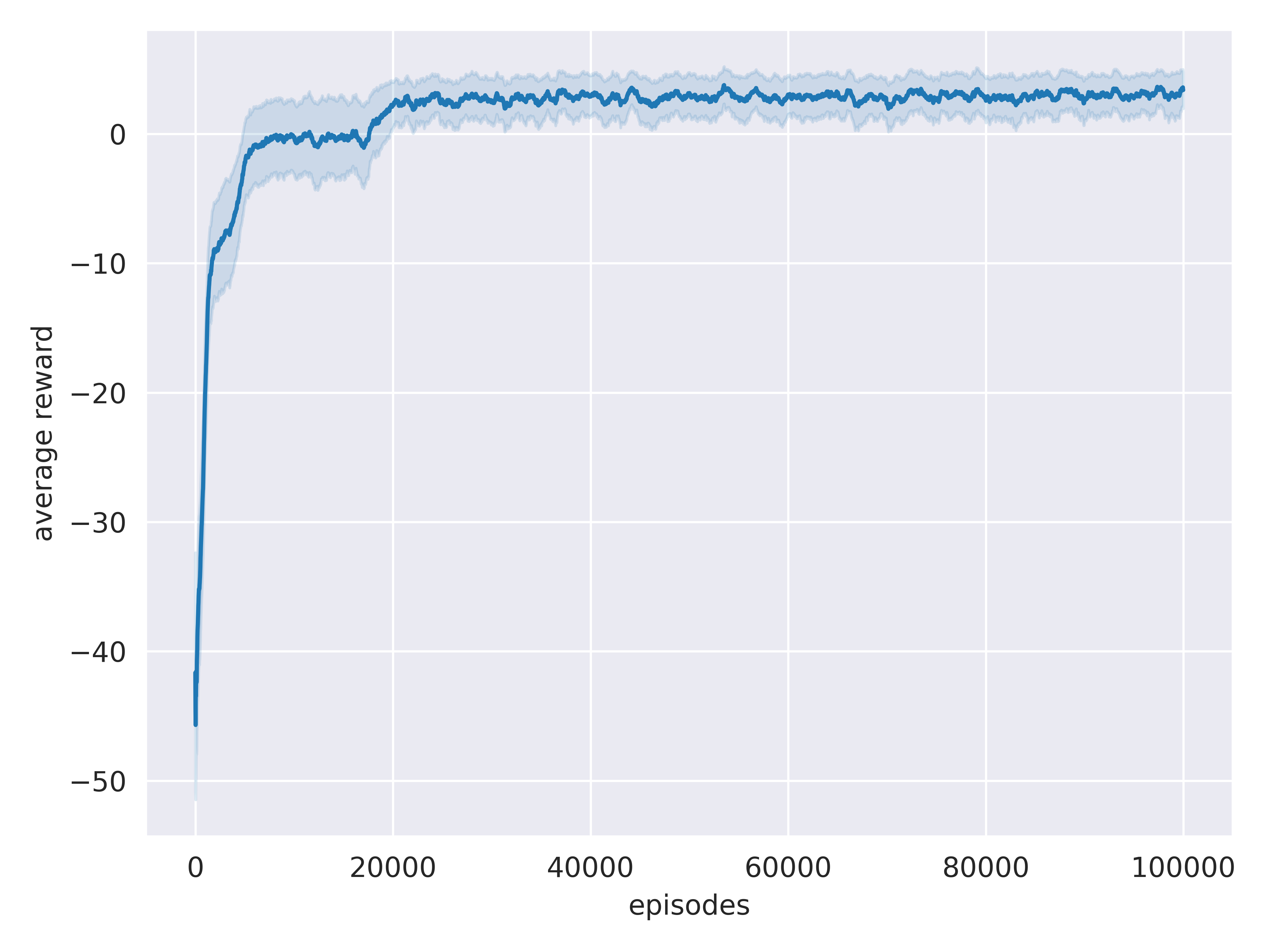
(a) Return on Tiger (lr=1e-4, number of particles=30).

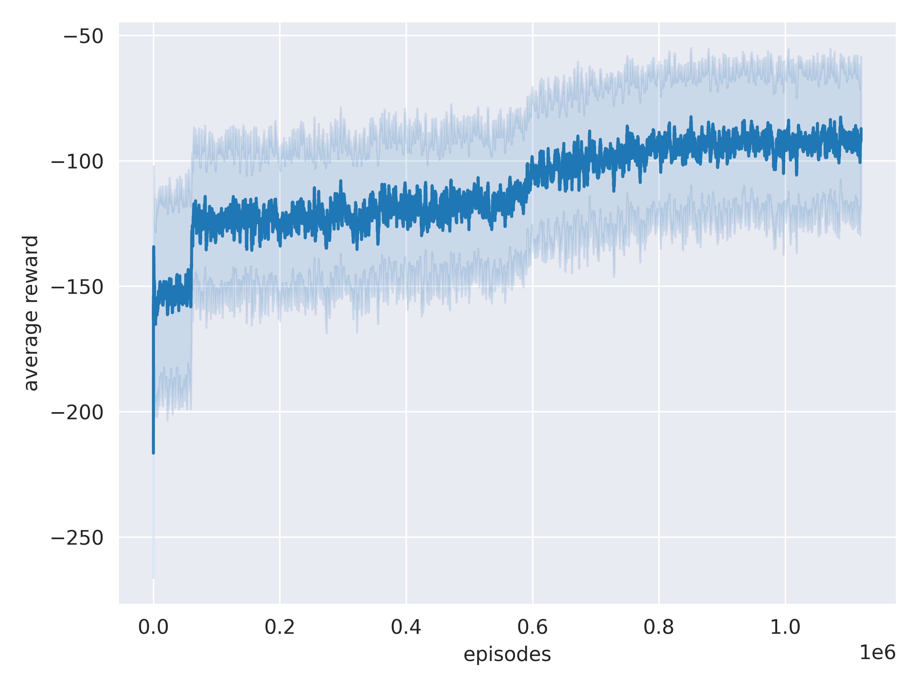
(b) Return on Collision-Avoidance (lr=1e-4, number of particles=30).

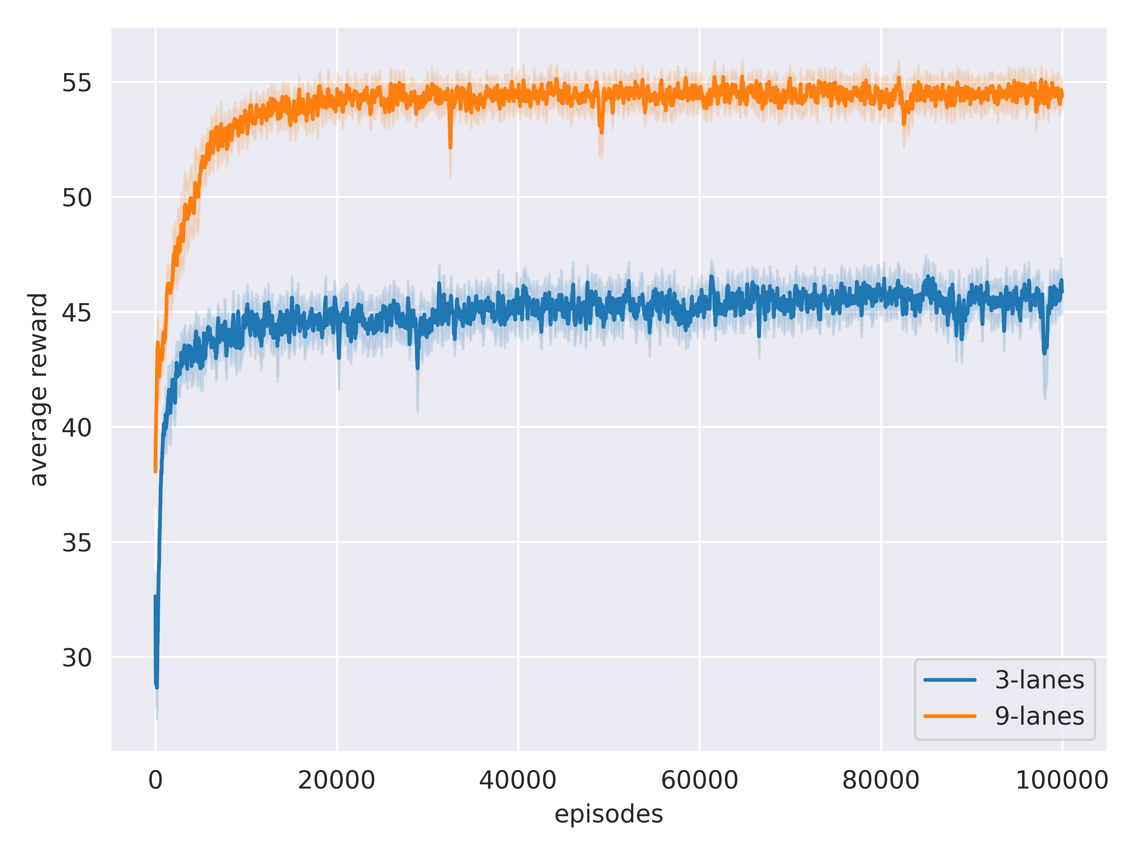
(a) Return on Road-Race: 3-lane (lr=1e-3, number of particles=15) and 9-lane (lr=3e-4, number of particles=15).

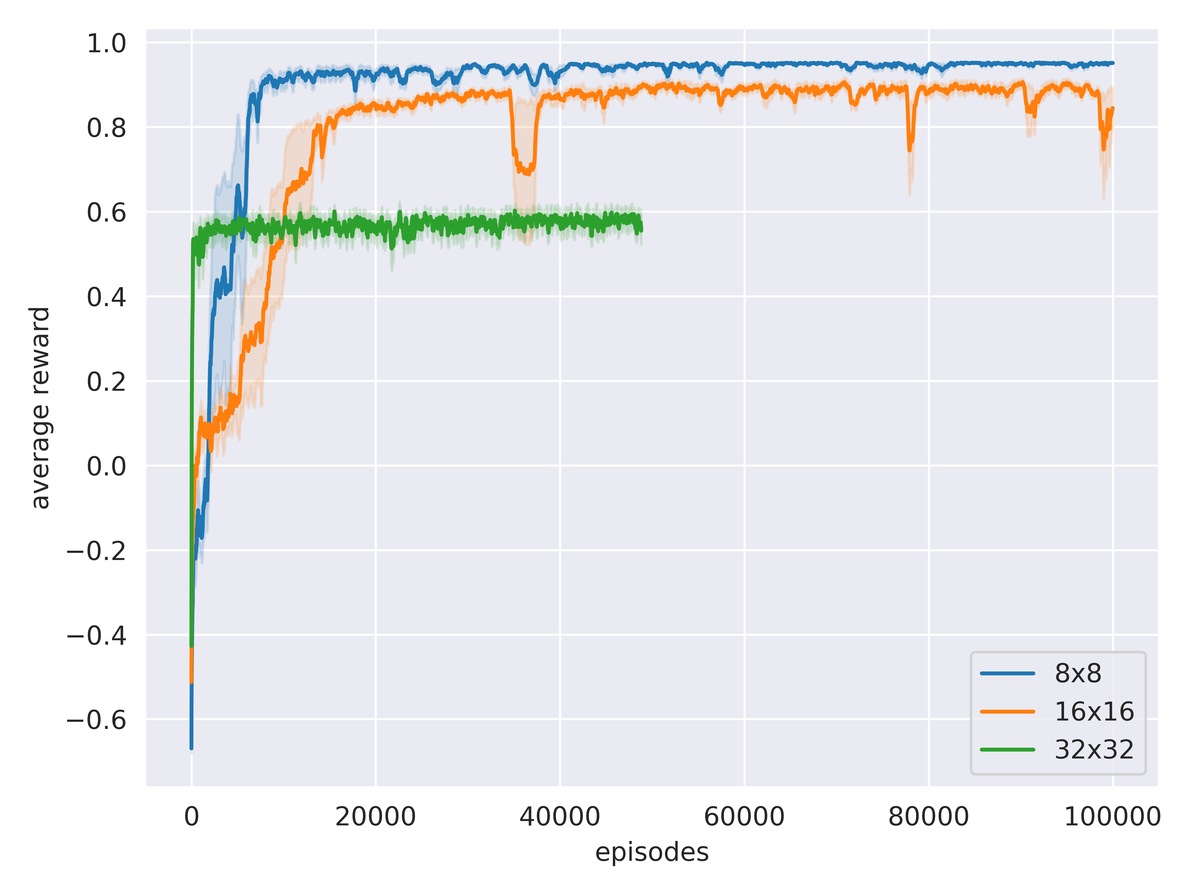
(b) Return on Grid-Verse of different sizes: 8x8 (lr=1e-3, number of particles=30), 16x16 (lr=1e-3, number of particles=30), 32x32 (lr=1e-3, number of particles=15).

In Table 6, we compare the number of episodes that DPFRL and BADDR took to achieve the same performance.

Domain	# Episodes for DFPRL	# Episodes for BADDr	Return Achieved
Tiger	20k	400	2.2
Collision-Avoidance	0.6M	500	-102
3-lane Road-Race	20k	200	45.2
9-lane Road-Race	8k	200	52.3
Grid-Verse (8x8)	5.95k	50	0.8
Grid-Verse (16x16)	13k	50	0.62
Grid-Verse (32x32)	N/A	50	0.62

Table 6. Comparison between the number of episodes needed for DPFRL and BADDr to achieve the same return.

References

- (1)
- Auer et al. (2002) Peter Auer, Nicolo Cesa-Bianchi, and Paul Fischer. 2002. Finite-time analysis of the multiarmed bandit problem. In Machine learning.
- Azizzadenesheli et al. (2018) Kamyar Azizzadenesheli, Emma Brunskill, and Animashree Anandkumar. 2018. Efficient exploration through Bayesian deep Q-networks. In 2018 Information Theory and Applications Workshop (ITA).
- Bellemare et al. (2016) Marc Bellemare, Sriram Srinivasan, Georg Ostrovski, Tom Schaul, David Saxton, and Remi Munos. 2016. Unifying count-based exploration and intrinsic motivation. In Advances in Neural Information Processing Systems.
- Browne et al. (2012) Cameron B. Browne, Edward Powley, Daniel Whitehouse, Simon M. Lucas, Peter I. Cowling, Philipp Rohlfshagen, Stephen Tavener, Diego Perez, Spyridon Samothrakis, and Simon Colton. 2012. A survey of Monte Carlo tree search methods. In IEEE Transactions on Computational Intelligence and AI in games, Vol. 4.
- Chua et al. (2018) Kurtland Chua, Roberto Calandra, Rowan McAllister, and Sergey Levine. 2018. Deep reinforcement learning in a handful of trials using probabilistic dynamics models. In Advances in Neural Information Processing Systems.
- Dallaire et al. (2009) Patrick Dallaire, Camille Besse, Stephane Ross, and Brahim Chaib-draa. 2009. Bayesian reinforcement learning in continuous POMDPs with Gaussian processes. In 2009 IEEE/RSJ International Conference on Intelligent Robots and Systems.
- Damianou and Lawrence (2013) Andreas Damianou and Neil D Lawrence. 2013. Deep Gaussian processes. In Artificial intelligence and statistics. PMLR, 207–215.
- Deisenroth and Rasmussen (2011) Marc Deisenroth and Carl E Rasmussen. 2011. PILCO: A model-based and data-efficient approach to policy search. In Proceedings of the International Conference on Machine Learning. Citeseer, 465–472.
- Deisenroth and Peters (2012) Marc Peter Deisenroth and Jan Peters. 2012. Solving nonlinear continuous state-action-observation POMDPs for mechanical systems with Gaussian noise. In The 10th European Workshop on Reinforcement Learning.
- Dietterich (2000) Thomas G. Dietterich. 2000. Ensemble methods in machine learning. In Multiple Classifier Systems (Lecture Notes in Computer Science). Springer Berlin Heidelberg.
- Doshi-Velez (2009) Finale Doshi-Velez. 2009. The infinite partially observable Markov decision process. In Advances in Neural Information Processing Systems.
- Duff and Barto (2002) Michael O’Gordon Duff and Andrew Barto. 2002. Optimal Learning: Computational procedures for Bayes-adaptive Markov decision processes. PhD Thesis. University of Massachusetts at Amherst.
- Gal and Ghahramani (2016) Yarin Gal and Zoubin Ghahramani. 2016. Dropout as a Bayesian approximation: Representing model uncertainty in deep learning. In Proceedings of the International Conference on Machine Learning.
- Gal et al. (2016) Yarin Gal, Rowan McAllister, and Carl Edward Rasmussen. 2016. Improving PILCO with Bayesian neural network dynamics models. In Data-Efficient Machine Learning workshop, ICML, Vol. 4. 25.
- Ghavamzadeh et al. (2016) Mohammad Ghavamzadeh, Shie Mannor, Joelle Pineau, and Aviv Tamar. 2016. Bayesian reinforcement learning: A survey. arXiv preprint arXiv:1609.04436 (2016).
- Guez (2015) A. G. Guez. 2015. Sample-based search methods for Bayes-adaptive planning. PhD Thesis. UCL (University College London).
- Ha and Schmidhuber (2018) David Ha and Jürgen Schmidhuber. 2018. World models. arXiv preprint arXiv:1803.10122 (2018).
- Hafner et al. (2020) Danijar Hafner, Timothy Lillicrap, Mohammad Norouzi, and Jimmy Ba. 2020. Mastering atari with discrete world models. In International Conference on Learning Representations.
- Hasselt et al. (2016) Hado Van Hasselt, Arthur Guez, and David Silver. 2016. Deep reinforcement learning with double Q-learning. In Proceedings of the AAAI Conference on Artificial Intelligence.
- Hausknecht and Stone (2015) Matthew Hausknecht and Peter Stone. 2015. Deep recurrent Q-learning for partially observable MDPs. arXiv preprint arXiv:1507.06527 (2015).
- Hinton et al. (2012) Geoffrey E. Hinton, Nitish Srivastava, Alex Krizhevsky, Ilya Sutskever, and Ruslan R. Salakhutdinov. 2012. Improving neural networks by preventing co-adaptation of feature detectors. arXiv preprint arXiv:1207.0580 (2012).
- Igl et al. (2018) Maximilian Igl, Luisa Zintgraf, Tuan Anh Le, Frank Wood, and Shimon Whiteson. 2018. Deep Variational Reinforcement Learning for POMDPs. In Proceedings of the International Conference on Machine Learning.
- Janner et al. (2019) Michael Janner, Justin Fu, Marvin Zhang, and Sergey Levine. 2019. When to Trust Your Model: Model-Based Policy Optimization. Advances in Neural Information Processing Systems 32 (2019), 12519–12530.
- Jaulmes et al. (2005) Robin Jaulmes, Joelle Pineau, and Doina Precup. 2005. Learning in non-stationary partially observable Markov decision processes. In ECML Workshop on Reinforcement Learning in non-stationary environments, Vol. 25.
- Jaulmes et al. (2007) Robin Jaulmes, Joelle Pineau, and Doina Precup. 2007. A formal framework for robot learning and control under model uncertainty. In Proceedings 2007 IEEE International Conference on Robotics and Automation.
- Jonschkowski et al. (2018) Rico Jonschkowski, Divyam Rastogi, and Oliver Brock. 2018. Differentiable particle filters: End-to-end learning with algorithmic priors. arXiv preprint arXiv:1805.11122 (2018).
- Kaelbling et al. (1998) Leslie Pack Kaelbling, Michael L. Littman, and Anthony R. Cassandra. 1998. Planning and acting in partially observable stochastic domains. In Artificial intelligence, Vol. 101.
- Karkus et al. (2018) Peter Karkus, David Hsu, and Wee Sun Lee. 2018. Integrating Algorithmic Planning and Deep Learning for Partially Observable Navigation. arXiv preprint arXiv:1807.06696 (2018).
- Katt et al. (2017) Sammie Katt, Frans A Oliehoek, and Christopher Amato. 2017. Learning in POMDPs with Monte Carlo tree search. In Proceedings of the International Conference on Machine Learning.
- Katt et al. (2019) Sammie Katt, Frans A. Oliehoek, and Christopher Amato. 2019. Bayesian Reinforcement Learning in Factored POMDPs. In Autonomous Agents and MultiAgent Systems.
- Kocsis and Szepesvári (2006) Levente Kocsis and Csaba Szepesvári. 2006. Bandit based Monte-Carlo planning. In European conference on machine learning. Springer.
- Li and Gal (2017) Yingzhen Li and Yarin Gal. 2017. Dropout inference in Bayesian neural networks with alpha-divergences. In Proceedings of the International Conference on Machine Learning.
- Luo et al. (2019) Yuanfu Luo, Haoyu Bai, David Hsu, and Wee Sun Lee. 2019. Importance sampling for online planning under uncertainty. In The International Journal of Robotics Research, Vol. 38.
- Ma et al. (2020) Xiao Ma, Peter Karkus, David Hsu, Wee Sun Lee, and Nan Ye. 2020. Discriminative particle filter reinforcement learning for complex partial observations. In International Conference on Learning Representations.
- McAllister and Rasmussen (2017) Rowan McAllister and Carl Edward Rasmussen. 2017. Data-efficient reinforcement learning in continuous state-action Gaussian-POMDPs. In Advances in Neural Information Processing Systems.
- Mnih et al. (2013) Volodymyr Mnih, Koray Kavukcuoglu, David Silver, Alex Graves, Ioannis Antonoglou, Daan Wierstra, and Martin Riedmiller. 2013. Playing Atari with deep reinforcement learning. arXiv preprint arXiv:1312.5602 (2013).
- Osband et al. (2018) Ian Osband, John Aslanides, and Albin Cassirer. 2018. Randomized prior functions for deep reinforcement learning. In Advances in Neural Information Processing Systems.
- Poupart and Vlassis (2008) Pascal Poupart and Nikos Vlassis. 2008. Model-based Bayesian reinforcement learning in partially observable domains. In Proc Int. Symp. on Artificial Intelligence and Mathematics,.
- Rajeswaran et al. (2017) Aravind Rajeswaran, Sarvjeet Ghotra, Balaraman Ravindran, and Sergey Levine. 2017. Epopt: Learning robust neural network policies using model ensembles. In International Conference on Learning Representations.
- Ross et al. (2008) Stephane Ross, Brahim Chaib-draa, and Joelle Pineau. 2008. Bayesian reinforcement learning in continuous POMDPs with application to robot navigation. In 2008 IEEE International Conference on Robotics and Automation.
- Ross et al. (2011) Stéphane Ross, Joelle Pineau, Brahim Chaib-draa, and Pierre Kreitmann. 2011. A Bayesian approach for learning and planning in partially observable Markov decision processes. In Journal of Machine Learning Research, Vol. 12. Issue May.
- Silver et al. (2016) David Silver, Aja Huang, Chris J. Maddison, Arthur Guez, Laurent Sifre, George Van Den Driessche, Julian Schrittwieser, Ioannis Antonoglou, Veda Panneershelvam, and Marc Lanctot. 2016. Mastering the game of Go with deep neural networks and tree search. In Nature, Vol. 529.
- Silver and Veness (2010) David Silver and Joel Veness. 2010. Monte-Carlo planning in large POMDPs. In Advances in Neural Information Processing Systems.
- Slade et al. (2017) Patrick Slade, Preston Culbertson, Zachary Sunberg, and Mykel Kochenderfer. 2017. Simultaneous active parameter estimation and control using sampling-based Bayesian reinforcement learning. In IEEE/RSJ International Conference on Intelligent Robots and Systems. 804–810. https://doi.org/10.1109/IROS.2017.8202242
- Srivastava et al. (2014) Nitish Srivastava, Geoffrey Hinton, Alex Krizhevsky, Ilya Sutskever, and Ruslan Salakhutdinov. 2014. Dropout: a simple way to prevent neural networks from overfitting. In The journal of machine learning research, Vol. 15.
- Sutton and Barto (1998) Richard S. Sutton and Andrew G. Barto. 1998. Introduction to reinforcement learning. Vol. 2.
- Thrun (2000) Sebastian Thrun. 2000. Monte Carlo POMDPs. In Advances in Neural Information Processing Systems.
- Wierstra et al. (2007) Daan Wierstra, Alexander Foerster, Jan Peters, and Juergen Schmidhuber. 2007. Solving deep memory POMDPs with recurrent policy gradients. In International Conference on Artificial Neural Networks. Springer.
- Wyatt (2001) Jeremy L. Wyatt. 2001. Exploration control in reinforcement learning using optimistic model selection. In Proceedings of the International Conference on Machine Learning.
- Yu et al. (2020) Tianhe Yu, Garrett Thomas, Lantao Yu, Stefano Ermon, James Y Zou, Sergey Levine, Chelsea Finn, and Tengyu Ma. 2020. MOPO: Model-based Offline Policy Optimization. Advances in Neural Information Processing Systems 33 (2020), 14129–14142.
- Zintgraf et al. (2019) Luisa Zintgraf, Kyriacos Shiarlis, Maximilian Igl, Sebastian Schulze, Yarin Gal, Katja Hofmann, and Shimon Whiteson. 2019. VariBAD: A Very Good Method for Bayes-Adaptive Deep RL via Meta-Learning. In International Conference on Learning Representations.