Abstract

We revisit the classical problem of deriving convergence rates for the maximum likelihood estimator (MLE) in finite mixture models. The Wasserstein distance has become a standard loss function for the analysis of parameter estimation in these models, due in part to its ability to circumvent label switching and to accurately characterize the behaviour of fitted mixture components with vanishing weights. However, the Wasserstein distance is only able to capture the worst-case convergence rate among the remaining fitted mixture components. We demonstrate that when the log-likelihood function is penalized to discourage vanishing mixing weights, stronger loss functions can be derived to resolve this shortcoming of the Wasserstein distance. These new loss functions accurately capture the heterogeneity in convergence rates of fitted mixture components, and we use them to sharpen existing pointwise and uniform convergence rates in various classes of mixture models. In particular, these results imply that a subset of the components of the penalized MLE typically converge significantly faster than could have been anticipated from past work. We further show that some of these conclusions extend to the traditional MLE. Our theoretical findings are supported by a simulation study to illustrate these improved convergence rates.

1 Introduction

Finite mixture models form a celebrated tool for modelling heterogeneous data, and are used pervasively in the life and physical sciences (Bechtel et al.,, 1993; Kuusela et al.,, 2012; McLachlan and Peel,, 2004). The primary goal in many such applications is to perform statistical inference for the mixture parameters. This raises the classical question of characterizing the optimal convergence rates for parameter estimation in finite mixture models. Though this topic has been the subject of considerable investigation in past literature, the aim of our work is to show how these existing results may be refined through a careful choice of the loss function used in their analyses.

Mixture distributions do not enjoy the standard regularity conditions that are typically presumed in parametric models, such as non-degeneracy of the Fisher information. As a result, optimal rates of estimation in mixtures are strictly slower than the usual parametric rate of convergence. This observation dates back at least to the seminal work of Chen, (1995), who analyzed univariate mixtures satisfying a regularity condition known as strong identifiability, which we formally define in Section 2 below. A long line of recent work has further analyzed convergence rates in mixtures of general dimension, under varying degrees of strong identifiability. In particular, Nguyen, (2013) proposed the Wasserstein distance as a natural tool for metrizing convergence of parameters in finite mixtures, via their mixing measure. The Wasserstein metric was then used to analyze convergence rates for the maximum likelihood estimator (MLE) and related procedures, under various classes of finite mixture models (Ho and Nguyen, 2016b, ; Ho and Nguyen, 2016a, ; Heinrich and Kahn,, 2018; Ho and Nguyen,, 2019). Moment-based estimators were also studied by Wu and Yang, (2020); Doss et al., (2020), and Bayesian estimators by Ohn and Lin, (2020); Guha et al., (2021), to name a few.

A broad conclusion of these works is that slow convergence rates are pervasive to parameter estimation in finite mixture models. This observation contrasts the fact that the minimax rate of estimating the density of a finite mixture model is typically the standard parametric rate of convergence (Genovese and Wasserman,, 2000; Ghosal and van der Vaart,, 2001; Doss et al.,, 2020; Ashtiani et al.,, 2020). For example, Heinrich and Kahn, (2018) show that the minimax rate for parameter estimation in a strongly identifiable mixture degrades exponentially as the number of components increases, when no separation conditions are placed on these components. This result suggests that the estimation of mixture parameters can be prohibitive, even when the number of components is moderate. On the other hand, practitioners have long been employing mixture models successfully, suggesting a discrepancy between practice and the worst-case rates suggested by the theory.

The goal of this paper is to revisit existing convergence rates for parameter estimation in finite mixture models, and to show that they may be refined by using stronger loss functions than the Wasserstein distance. We will argue that the Wasserstein distance is only able to capture the worst-case convergence rate among the estimated components of a mixture, and that in many cases, the vast majority of estimated component parameters may achieve considerably faster convergence rates than anticipated from prior work. Before describing these phenomena in further detail, we begin by formally introducing finite mixture models and related notions.

1.1 Problem Setting

Finite Mixture Models. Let $\mathcal{F}=\{f(x|\theta):x\in\mathcal{X},\theta\in\Theta\}$ be a known parametric family of density functions with respect to a dominating $\sigma$-finite measure $\nu$. Here, we assume $\mathcal{X}\subseteq\mathbb{R}^{N}$ for some $N\geq 1$, and $\Theta$ is a parameter space which will either be a subset of the Euclidean space $\mathbb{R}^{d}$, $d\geq 1$, or of the set $\mathbb{R}^{d}\times\mathbb{S}^{d}_{++}$, where $\mathbb{S}^{d}_{++}$ denotes the cone of $d\times d$ positive definite matrices. In either case, we shall always tacitly assume that $\Theta$ is a compact set with nonempty interior. Let $X_{1},X_{2},\ldots,X_{n}$ be an i.i.d. sample from a finite mixture model with $k_{0}\geq 1$ components, whose density with respect to $\nu$ is written as

$$p_{G_{0}}(x):=\int f(x|\theta)dG_{0}(\theta)=\sum_{j=1}^{k_{0}}p_{j}^{0}f(x|\theta_{j}^{0}),\quad x\in\mathcal{X}.$$

Here $G_{0}=\sum_{j=1}^{k_{0}}p_{j}^{0}\delta_{\theta_{j}^{0}}$ denotes an unknown mixing measure, where the $p_{j}^{0}\geq 0$ are called mixing proportions (or weights), satisfying $\sum_{j=1}^{k_{0}}p_{j}^{0}=1$, and the $\theta_{j}^{0}\in\Theta$ are called atoms, for $j=1,\dots,k_{0}$. When the mixing proportions are strictly positive and the atoms are distinct, we say $G_{0}$ has true order $k_{0}$. More generally, any finitely-supported probability measure on $\Theta$ is called a mixing measure, and its support size is called its order. The set of mixing measures of order at most $k\geq 1$ is denoted $\mathcal{O}_{k}(\Theta)$, and we write $\mathcal{E}_{k}(\Theta)=\mathcal{O}_{k}(\Theta)\setminus\mathcal{O}_{k-1}(\Theta)$.

When dealing with parameter estimation in a finite mixture model, it is convenient to treat the mixing measure $G_{0}$ as the target of estimation, even if the main quantities of interest are the mixing proportions or atoms of $G_{0}$. Indeed, while the density $p_{G}$ is typically identifiable with respect to its mixing measure $G$, it is never identifiable with respect to the individual parameters of $G$, due to the possibility of label-switching. Throughout our work, we will consider both pointwise rates of estimating the mixing measure, that is, estimation rates which depend on the fixed mixing measure $G_{0}$, and uniform estimation rates, which hold uniformly over all mixing measures under consideration. We will always emphasize the latter setting by allowing $G_{0}\equiv G_{0}^{n}$ to potentially depend on the sample size $n$.

Maximum Likelihood Estimation. Perhaps the most widely-used estimator of $G_{0}$ is the maximum likelihood estimator (MLE). We focus our analysis on estimators based on the MLE throughout this work, in part because they allow for a general theory of parameter estimation to be derived under minimal conditions on the family $\mathcal{F}$. Given an integer $k\geq 1$, the MLE of $G_{0}$ with order at most $k$ is given by

$$\macc@depth\char 1\relax\frozen@everymath{\macc@group}\macc@set@skewchar\macc@nested@a 111{G}_{n} =\sum_{i=1}^{\macc@depth\char 1\relax\frozen@everymath{\macc@group}\macc@set@skewchar\macc@nested@a 111{k}_{n}}\macc@depth\char 1\relax\frozen@everymath{\macc@group}\macc@set@skewchar\macc@nested@a 111{p}_{i}^{n}\delta_{\macc@depth\char 1\relax\frozen@everymath{\macc@group}\macc@set@skewchar\macc@nested@a 111{}_{i}^{n}}=\operatorname*{argmax}_{G\in\mathcal{O}_{k}(\Theta)}\ell_{n}(G),\qquad\text{where }\ell_{n}(G)=\sum_{i=1}^{n}\log p_{G}(X_{i}).$$ (1)

Here, $\bar{k}_{n}\leq k$ denotes the fitted order of $\macc@depth\char 1\relax\frozen@everymath{\macc@group}\macc@set@skewchar\macc@nested@a 111{G}_{n}$. We have defined the MLE with the general order $k$ to reflect the fact that true order $k_{0}$ of $G_{0}$ may be unknown. Notice that $\macc@depth\char 1\relax\frozen@everymath{\macc@group}\macc@set@skewchar\macc@nested@a 111{G}_{n}$ is generally inconsistent if $k<k_{0}$, thus we shall always assume $k\geq k_{0}$. Our convergence rates will depend on the level of misspecification $k-k_{0}$.

In certain parts of our development, it will be technically convenient to ensure that the fitted mixing proportions of $\macc@depth\char 1\relax\frozen@everymath{\macc@group}\macc@set@skewchar\macc@nested@a 111{G}_{n}$ do not vanish. While this can be achieved by constraining the maximum in equation (1), we will prefer to achieve this using a penalty on the likelihood function. Specifically, we follow Chen and Kalbfleisch, (1996) and define the penalized MLE of order at most $k$ by

$$\widehat{G}_{n}=\sum_{i=1}^{\widehat{k}_{n}}\widehat{p}_{i}^{n}\delta_{\widehat{\theta}_{i}^{n}}=\operatorname*{argmax}_{G\in\mathcal{O}_{k}(\Theta)}\ell_{n}(G)+\xi_{n}\rho(G),$$

where $\widehat{k}_{n}\leq k$ is the order of $\widehat{G}_{n}$, $\xi_{n}\geq 0$ is a tuning parameter, and $\rho$ satisfies $\rho(G)\to-\infty$ as the smallest mixing weight of $G$ vanishes. For concreteness, we will use the penalty $\rho(G)=\sum_{j=1}^{k^{\prime}}\log p_{j}^{\prime}$, where $k^{\prime}\leq k$ denotes the order of $G=\sum_{j=1}^{k^{\prime}}p_{j}^{\prime}\delta_{\theta_{j}^{\prime}}$. As discussed in Appendix C.1, with this choice of penalty, $\widehat{G}_{n}$ may be numerically approximated using a simple modification of the EM algorithm.

In order to evaluate the risk of the estimators $\widehat{G}_{n}$ and $\macc@depth\char 1\relax\frozen@everymath{\macc@group}\macc@set@skewchar\macc@nested@a 111{G}_{n}$, we will require loss functions defined over $\mathcal{O}_{k}(\Theta)$. The most widely-used loss function appearing in past work is the Wasserstein distance, which we define next.

Wasserstein Distances. Let $k,k^{\prime}\geq 1$, and set $G=\sum_{i=1}^{k}p_{i}\delta_{\theta_{i}}\in\mathcal{O}_{k}(\Theta)$ and $G^{\prime}=\sum_{j=1}^{k^{\prime}}p_{j}^{\prime}\delta_{\theta_{j}^{\prime}}\in\mathcal{O}_{k^{\prime}}(\Theta)$. Denote by $\Pi(G,G^{\prime})$ the set of joint probability mass functions $\mathbf{q}=(q_{ij}:i\in[k],j\in[k^{\prime}])$ admitting marginal distributions equal to those of $G$ and $G^{\prime}$, that is, $\sum_{i=1}^{k}q_{ij}=p_{j}^{\prime}$ and $\sum_{j=1}^{k^{\prime}}q_{ij}=p_{i}$, for all $i\in[k]$ and $j\in[k^{\prime}]$. The Wasserstein distance of order $r\geq 1$ is defined by

$$W_{r}(G,G^{\prime})=\left(\inf_{\mathbf{q}\in\Pi(G,G^{\prime})}\sum_{i=1}^{k}\sum_{j=1}^{k^{\prime}}q_{ij}D^{r}(\theta_{i},\theta_{j}^{\prime})\right)^{\frac{1}{r}},$$

where $D$ is a metric on $\Theta$. When $\Theta\subseteq\mathbb{R}^{d}$, we shall always assume that $D=\|\cdot\|$ is induced by the Euclidean norm.

The use of Wasserstein distances in general dimension originated from the work of Nguyen, (2013), and was partly motivated by its implication for the convergence of atoms, as we now recall. Let $G_{n}\in\mathcal{O}_{k}(\Theta)$ be a sequence of mixing measures, and $G_{0}\in\mathcal{E}_{k_{0}}(\Theta)$. Then, if $W_{r}(G_{n},G_{0})\leq\alpha_{n}$ for some $\alpha_{n}\downarrow 0$, there exists a subsequence of $G_{n}$ such that every atom $\theta_{j}^{0}$ of $G_{0}$ is the limit point of at least one atom $\theta_{i}^{n}$ of $G_{n}$. Furthermore, the convergence rate of this fitted atom is $D(\theta_{i}^{n},\theta_{j}^{0})\lesssim\alpha_{n}$. When $k>k_{0}$, there may also be atoms $\theta_{\ell}^{n}$ of $G_{n}$ which do not converge to any atoms of $G_{0}$. It can be seen that their corresponding mixing proportions $p_{\ell}^{n}$ must then vanish at the rate $\alpha_{n}^{r}$. If we instead assume that the mixing proportions of $G_{n}$ are bounded from below by a positive constant $c_{0}>0$, it must in fact hold that every atom of $G_{n}$ converges to an atom of $G_{0}$ at rate $\alpha_{n}$.

We note in particular that the Wasserstein distance can only induce the same convergence rate $\alpha_{n}$ for those atoms of $G_{n}$ which approach the atoms of $G_{0}$. In contrast, a key observation of our work is that maximum likelihood-based estimators have atoms which converge at distinct rates; such heterogeneous behaviour cannot be captured by the Wasserstein distance, and is the main subject of this paper.

1.2 Contributions

Our goal is to provide sharper rates of convergence for parameter estimation in finite mixture models of various types. Our main technical contribution is the development of loss functions over the space of mixing measures, which are stronger than the Wasserstein distance, and which correctly characterize the heterogeneous convergence rates of the various mixture parameters in maximum likelihood-based estimators. To illustrate the refinements furnished by our theory, we consider the following example.

Example 1 (Pointwise Convergence Rates for Strongly Identifiable Mixtures).

Suppose $\mathcal{F}$ is the location family of Gaussian densities with known variance. Furthermore, assume $k=k_{0}+1$. The works of Chen, (1995); Ho and Nguyen, 2016b show there exists a constant $C(G_{0})>0$ such that

$$\mathbb{E}W_{2}(\macc@depth\char 1\relax\frozen@everymath{\macc@group}\macc@set@skewchar\macc@nested@a 111{G}_{n},G_{0})\leq C(G_{0})(\log n/n)^{1/4}.$$

In particular, it follows that for every atom $\theta_{j}^{0}$ of $G_{0}$, there is at least one atom of $\macc@depth\char 1\relax\frozen@everymath{\macc@group}\macc@set@skewchar\macc@nested@a 111{G}_{n}$ which converges to $\theta_{j}^{0}$ at the pointwise rate $(\log n/n)^{1/4}$. Equivalently, there exists an injection $u_{n}:[k_{0}]\to[k]$ such that

$$\max_{1\leq j\leq k_{0}}\mathbb{E}\|\macc@depth\char 1\relax\frozen@everymath{\macc@group}\macc@set@skewchar\macc@nested@a 111{}_{u_{n}(j)}^{n}-\theta_{j}^{0}\|\leq C(G_{0})\left(\log n/n\right)^{\frac{1}{4}}.$$ (2)

In contrast, it will follow from our Theorem 4 below that there exists an injection $v_{n}:[k_{0}]\to[k]$ and a permutation $\sigma_{n}:[k_{0}]\to[k_{0}]$ such that

$$\max_{1\leq j\leq k_{0}-1}\mathbb{E}\|\macc@depth\char 1\relax\frozen@everymath{\macc@group}\macc@set@skewchar\macc@nested@a 111{}_{v_{n}(j)}^{n}-\theta_{\sigma_{n}(j)}^{0}\| \leq C(G_{0})\left(\frac{\log n}{n}\right)^{\frac{1}{2}},$$

$$\mathbb{E}\|\macc@depth\char 1\relax\frozen@everymath{\macc@group}\macc@set@skewchar\macc@nested@a 111{}_{v_{n}(k_{0})}^{n}-\theta_{\sigma_{n}(k_{0})}^{0}\| \leq C(G_{0})\left(\frac{\log n}{n}\right)^{\frac{1}{4}}.$$

This result shows that, ignoring polylogarithmic factors, all but two of the atoms of the overfitted MLE $\macc@depth\char 1\relax\frozen@everymath{\macc@group}\macc@set@skewchar\macc@nested@a 111{G}_{n}$ achieve the parametric convergence rate. In contrast, equation (2) merely shows that these atoms converge at the slower rate $(\log n/n)^{1/4}$.

We will show that similar asymptotics hold for a broad family of strongly identifiable mixture models, and for general $k\geq k_{0}$, in Section 3.1, We further consider uniform convergence rates for such families in Section 4, as well as pointwise convergence rates for location-scale Gaussian mixture models (Section 3.2), which form an important example of weakly identifiable finite mixtures. We obtain these results by identifying distinct loss functions tailored to each of these three settings, which accurately capture the behaviour of individual fitted mixture parameters.

Our results highlight the underappreciated fact that the Wasserstein distance merely quantifies the worst-case convergence rate among the fitted parameters of a finite mixture; its use in past work may thus have painted an overly pessimistic picture of parameter estimation in these models. Though our primary emphasis is on such theoretical aspects, we will also discuss that certain loss functions developed in this work enjoy an improved computational complexity as compared to the Wasserstein distance, and may therefore be of practical significance in their own right.

Notation. Given probability densities $p,q$ dominated by $\nu$, their squared Hellinger and Total Variation distances are denoted by $h^{2}(p,q)=\frac{1}{2}\int(\sqrt{p}-\sqrt{q})^{2}d\nu$ and $V(p,q)=\frac{1}{2}\int|p-q|d\nu$. $\mathcal{O}_{k,c_{0}}(\Theta)$ denotes the set of mixing measures in $\mathcal{O}_{k}(\Theta)$ with mixing weights bounded below by a constant $c_{0}>0$, and $\mathcal{E}_{k,c_{0}}(\Theta)=\mathcal{O}_{k,c_{0}}(\Theta)\setminus\mathcal{O}_{k-1}(\Theta)$. For any $n\geq 1$, we denote $[n]=\{1,2,\ldots,n\}$. For any $a,b\in\mathbb{R}$, $a\vee b=\max\{a,b\}$ and $a\wedge b=\min\{a,b\}$. Given $(a_{n})_{n\geq 1},(b_{n})_{n\geq 1}\subseteq\mathbb{R}_{+}$, we write $a_{n}\lesssim b_{n}$ if there exists a universal constant $C>0$, possibly depending on problem parameters to be understood from context, such that $a_{n}\leq Cb_{n}$ for all $n\geq 1$. We also write $a_{n}\asymp b_{n}$ when $a_{n}\lesssim b_{n}\lesssim a_{n}$. $\mathcal{C}^{\alpha}(\Theta)$ denotes the Hölder space of regularity $\alpha>0$ over $\Theta$, with associated norm $\|\cdot\|_{\mathcal{C}^{\alpha}(\Theta)}$ (Folland,, 1995).

2 Preliminaries

2.1 Strong Identifiability

We begin by recalling the strong identifiability condition for the parametric family $\mathcal{F}$.

Definition 1 (Strong Identifiability).

Let $r\geq 0$ be an integer. We say $\mathcal{F}$ is $r$-strongly identifiable if $f(x|\cdot)\in\mathcal{C}^{r}(\Theta)$ for $\nu$-almost every $x\in\mathcal{X}$, and if for any $k\geq 1$, and $\theta_{1},\dots,\theta_{k}\in\Theta$, the following implication holds for all $\alpha_{\eta}^{(i)}\in\mathbb{R}$,

$$\operatorname*{esssup}_{x\in\mathcal{X}}\Bigg{|}\sum_{\ell=0}^{r}\sum_{|\eta|=\ell}\sum_{i=1}^{k}\alpha_{\eta}^{(i)}\frac{\partial^{|\eta|}f}{\partial\theta^{\eta}}(x|\theta_{i})\Bigg{|}=0\Longrightarrow\max_{|\eta|\leq r}\max_{1\leq i\leq k}|\alpha_{\eta}^{(i)}|=0.$$

The notion of strong identifiability originates from the work of Chen, (1995), and is stated here in a more general form due to Heinrich and Kahn, (2018); Ho and Nguyen, 2016b . We refer to these references, as well as that of Holzmann et al., (2004), for sufficient conditions under which the strong identifiability condition holds. For example, this condition is known to be satisfied for any finite $r\geq 1$ by the location Gaussian parametric family with known scale parameter, the Poisson family, and other common exponential families. Location-scale Gaussian densities form perhaps the most widely-used parametric family which fails to satisfy the $r$-strong identifiability condition for $r\geq 2$ Ho and Nguyen, 2016a , and we will treat this special case separately.

We will typically couple the strong identifiability condition with the following assumption on the modulus of continuity of the derivatives of $f(x|\cdot)$, up to order $r\geq 1$.

1. There exist $\Lambda,\delta>0$ such that

   $$\operatorname*{esssup}_{x\in\mathcal{X}}\|f(x|\cdot)\|_{\mathcal{C}^{r+\delta}(\Theta)}\leq\Lambda.$$

Strong identifiability generalizes the condition of regular identifiability of the family $\mathcal{P}_{k}(\Theta)=\{p_{G}:G\in\mathcal{O}_{k}(\Theta)\}$, and is a useful notion for deriving inequalities between Wasserstein-type distances over $\mathcal{O}_{k}(\Theta)$ and statistical distances over $\mathcal{P}_{k}(\Theta)$. Such bounds are at the heart of our proofs, and will allow us to derive parameter estimation rates from known convergence rates for maximum likelihood density estimation, to which we turn our attention next.

2.2 Convergence Rates for Maximum Likelihood Density Estimators

In order to state a rate of convergence for the density estimators $p_{\widehat{G}_{n}}$ and $p_{\macc@depth\char 1\relax\frozen@everymath{\macc@group}\macc@set@skewchar\macc@nested@a 111{G}_{n}}$, for instance under the Hellinger distance, we require a condition on the complexity of the class

$$\macc@depth\char 1\relax\frozen@everymath{\macc@group}\macc@set@skewchar\macc@nested@a 111{}_{k}^{1/2}(\Theta,\epsilon)=\left\{\bar{p}_{G}^{1/2}:G\in\mathcal{O}_{k}(\Theta),\leavevmode\nobreak\ h(\bar{p}_{G},p_{G_{0}})\leq\epsilon\right\},$$

where $\epsilon>0$, and for any $G\in\mathcal{O}_{k}(\Theta)$, we write $p_{G}=(p_{G}+p_{G_{0}})/2$. The definition of $\macc@depth\char 1\relax\frozen@everymath{\macc@group}\macc@set@skewchar\macc@nested@a 111{}_{k}^{1/2}(\Theta,\epsilon)$ originates from van de Geer, (2000), who place conditions on the convex combinations $\bar{p}_{G}$, rather than $p_{G}$, as this choice is guaranteed to place a non-negligible amount of probability mass over the support of $p_{G_{0}}$. The complexity of this class is measured through the bracketing entropy integral

$$\mathcal{J}_{B} (\epsilon,\macc@depth\char 1\relax\frozen@everymath{\macc@group}\macc@set@skewchar\macc@nested@a 111{}_{k}^{1/2}(\Theta,\epsilon),\nu){=}\int_{0}^{\epsilon}\sqrt{H_{B}(u,\macc@depth\char 1\relax\frozen@everymath{\macc@group}\macc@set@skewchar\macc@nested@a 111{}_{k}^{1/2}(\Theta,u),\nu)}du\leavevmode\nobreak\ {\vee}\epsilon,$$

where $H_{B}(\epsilon,\mathcal{P},\nu)$ denotes the $\epsilon$-bracketing entropy of a set $\mathcal{P}\subseteq L^{2}(\nu)$ with respect to the $L^{2}(\nu)$ metric (van de Geer,, 2000). We shall assume that this quantity satisfies the following condition.

1. Given a universal constant $J>0$, there exists a constant $L>0$, possibly depending on $d$ and $k$, such that for all $n\geq 1$ and all $\epsilon>L(\log n/n)^{1/2}$,

   $$\mathcal{J}_{B}(\epsilon,\macc@depth\char 1\relax\frozen@everymath{\macc@group}\macc@set@skewchar\macc@nested@a 111{}_{k}^{1/2}(\Theta,\epsilon),\nu)\leq J\sqrt{n}\epsilon^{2}.$$

We are now ready to state the following convergence rates.

Theorem 2.

Given $k\geq 1$, assume condition B($k$) holds.

1. There exists a constant $C>0$ depending only on $d,k,\mathcal{F}$ such that for all $n\geq 1$,

   $$\sup_{G_{0}\in\mathcal{O}_{k}(\Theta)}\mathbb{E}_{G_{0}}h(p_{\macc@depth\char 1\relax\frozen@everymath{\macc@group}\macc@set@skewchar\macc@nested@a 111{G}_{n}},p_{G_{0}})\leq C\sqrt{\frac{\log n}{n}}.$$

2. Furthermore, given $c_{0},c_{1}>0$, if $0\leq\xi_{n}\leq c_{1}\log n$, then there exists a constant $C^{\prime}>0$ depending on $d,k,c_{0},c_{1},\mathcal{F}$ such that for all $n\geq 1$,

   $$\sup_{G_{0}\in\mathcal{O}_{k,c_{0}}(\Theta)}\mathbb{E}_{G_{0}}h(p_{\widehat{G}_{n}},p_{G_{0}})\leq\frac{C^{\prime}\log n}{\sqrt{n}}.$$

Theorem 2(i) is a direct consequence of generic results for maximum likelihood density estimation (for instance, Theorem 7.4 of van de Geer, (2000)). Its application to finite mixture models has previously been discussed by Ho and Nguyen, 2016b , who also argue that condition B($k$) is satisfied by a broad collection of parametric families $\mathcal{F}$, including the multivariate location-scale Gaussian and Student-$t$ families. A version of Theorem 2(ii) is implicit in the work of Manole and Khalili, (2021), though with a stronger condition on the tuning parameter $\xi_{n}$. We provide a self-contained proof of this result in Appendix A for completeness.

These results may also be used to show that the penalized MLE has nonvanishing mixing proportions.

Proposition 3.

Let $k\geq 1$, $c_{0}\in(0,1)$, and assume condition B($k$) holds. Assume further that $\xi_{n}\geq\log n$. Then, there exists a constant $c>1$ depending on $c_{0},d,k,\mathcal{F}$ such that for all $n\geq 1$,

$$\sup_{G_{0}\in\mathcal{O}_{k,c_{0}}(\Theta)}\mathbb{P}_{G_{0}}\left(\min_{1\leq j\leq{\widehat{k}_{n}}}\widehat{p}_{j}^{n}\geq\frac{1}{c}\right)\leq\frac{c}{n}.$$

In view of Proposition 3 and Theorem 2, we shall always tacitly assume that the tuning parameter $\xi_{n}$ is equal to $\log n$.

3 Pointwise Convergence Rates of the MLE

We first derive pointwise convergence rates for estimating a fixed mixing measure $G_{0}\in\mathcal{E}_{k_{0}}(\Theta)$.

3.1 Strongly Identifiable Case

Assume the family $\mathcal{F}$ is twice strongly identifiable, with a compact parameter space $\Theta\subseteq\mathbb{R}^{d}$ admitting nonempty interior. We begin by defining a loss function on $\mathcal{O}_{k}(\Theta)$ tailored to this setting. Given a mixing measure $G=\sum_{i=1}^{k^{\prime}}p_{i}\delta_{\theta_{i}}$ of order $k^{\prime}\leq k$, we partition its atoms into the following Voronoi cells, generated by the support of $G_{0}$,

$$\mathcal{A}_{j}\equiv\mathcal{A}_{j}(G)=\{i\in[k^{\prime}]:\|\theta_{i}-\theta_{j}^{0}\|\leq\|\theta_{i}-\theta_{\ell}^{0}\|\ \forall\ell\neq j\},$$

for all $j\in[k_{0}]$. We may then define the loss function

$$\mathcal{D}(G,G_{0}):=\sum_{j:|\mathcal{A}_{j}|>1}\sum_{i\in\mathcal{A}_{j}}p_{i}\|\theta_{i}-\theta_{j}^{0}\|^{2}+\sum_{j:|\mathcal{A}_{j}|=1}\sum_{i\in\mathcal{A}_{j}}p_{i}\|\theta_{i}-\theta_{j}^{0}\|+\sum_{j=1}^{k_{0}}\left|\sum_{i\in\mathcal{A}_{j}}p_{i}-p_{j}^{0}\right|.$$ (3)

Clearly, $\mathcal{D}(G,G_{0}){=}0$ if and only if $G{=}G_{0}$. Under this loss function, we obtain the following bound on the risk of $\macc@depth\char 1\relax\frozen@everymath{\macc@group}\macc@set@skewchar\macc@nested@a 111{G}_{n}$.

Theorem 4.

Let $k\geq k_{0}$. Assume that the parametric family $\mathcal{F}$ is 2-strongly identifiable, and satisfies conditions A($2$) and B($k$). Then, there exists a constant $C(G_{0})>0$, depending on $G_{0},d,k,\mathcal{F}$, such that

$$\mathbb{E}\big{[}\mathcal{D}(\macc@depth\char 1\relax\frozen@everymath{\macc@group}\macc@set@skewchar\macc@nested@a 111{G}_{n},G_{0})\big{]}\leq C(G_{0})\sqrt{\frac{\log n}{n}}.$$

The proof of Theorem 4 appears in Appendix A.3, where the main difficulty is to prove the following lower bound of the Hellinger distance in terms of $\mathcal{D}$,

$$\mathcal{D}(G,G_{0})\leq C(G_{0})h(p_{G},p_{G_{0}}),$$ (4)

for any $G\in\mathcal{O}_{k}(\Theta)$. Using Theorem 2(i), the above bound directly leads to the stated convergence rate of $\macc@depth\char 1\relax\frozen@everymath{\macc@group}\macc@set@skewchar\macc@nested@a 111{G}_{n}$.

A few comments regarding Theorem 4 are in order. First, let $\mathcal{A}_{j}^{n}=\mathcal{A}_{j}(\macc@depth\char 1\relax\frozen@everymath{\macc@group}\macc@set@skewchar\macc@nested@a 111{G}_{n})$ for all $j\in[k_{0}]$. The convergence rate $\sqrt{\log n/n}$ of $\mathcal{D}(\macc@depth\char 1\relax\frozen@everymath{\macc@group}\macc@set@skewchar\macc@nested@a 111{G}_{n},G_{0})$ implies that for any index $j\in[k_{0}]$ such that $|\mathcal{A}_{j}^{n}|=1$, $\|\macc@depth\char 1\relax\frozen@everymath{\macc@group}\macc@set@skewchar\macc@nested@a 111{}_{i}^{n}-\theta_{j}^{0}\|$ and $|\macc@depth\char 1\relax\frozen@everymath{\macc@group}\macc@set@skewchar\macc@nested@a 111{p}_{i}^{n}-p_{i}^{0}|$ vanish at the near-parametric rate $\sqrt{\log n/n}$ for $i\in\mathcal{A}_{j}^{n}$. Therefore, among the true components which are only approximated by a single fitted component, the parameters of this fitted component converge as fast as if the order $k\geq k_{0}$ were not overspecifed. In particular, in the exact-fitted setting $k=k_{0}$, we find that all fitted components and mixing proportions converge at the parametric rate, up to a polylogarithmic factor, which recovers Theorem 3.1 of Ho and Nguyen, 2016b . Furthermore, when $k>k_{0}$, for any index $j\in[k_{0}]$ such that $|\mathcal{A}_{j}^{n}|\geq 2$, $\sum_{i\in\mathcal{A}_{j}^{n}}\macc@depth\char 1\relax\frozen@everymath{\macc@group}\macc@set@skewchar\macc@nested@a 111{p}_{i}^{n}\|\macc@depth\char 1\relax\frozen@everymath{\macc@group}\macc@set@skewchar\macc@nested@a 111{}_{i}^{n}-\theta_{j}^{0}\|^{2}$ and $|\sum_{i\in\mathcal{A}_{j}^{n}}\macc@depth\char 1\relax\frozen@everymath{\macc@group}\macc@set@skewchar\macc@nested@a 111{p}_{i}^{n}-p_{j}^{0}|$ decay at the rate $\sqrt{\log n/n}$. In particular, it follows that for every such $j$, there exists $i\in\mathcal{A}_{j}^{n}$ such that $\macc@depth\char 1\relax\frozen@everymath{\macc@group}\macc@set@skewchar\macc@nested@a 111{}_{i}^{n}$ converges to $\theta_{j}^{0}$ at the rate $(\log n/n)^{1/4}$, which is now markedly slower than the parametric rate. In contrast, the past works of Chen, (1995); Nguyen, (2013); Ho and Nguyen, 2016b show that $\mathbb{E}W_{2}^{2}(\macc@depth\char 1\relax\frozen@everymath{\macc@group}\macc@set@skewchar\macc@nested@a 111{G}_{n},G_{0})\lesssim\sqrt{\log n/n}$, which implies a convergence rate no better than $(\log n/n)^{1/4}$ for all atoms of the MLE, rather than just those lying in a set $\mathcal{A}_{j}^{n}$ with cardinality greater than one. These existing results painted a pessimistic picture of maximum likelihood estimation in overspecified mixtures—for example, they suggest that overspecifying the order $k_{0}$ merely by $k=k_{0}+1$ leads to poor convergence rates for each of the $k$ fitted atoms, whereas our work shows that at least $k_{0}-1$ fitted atoms enjoy considerably faster convergence rates.

Second, we can demonstrate that $\mathcal{D}\gtrsim W_{2}^{2}$, and

$$\sup_{\begin{subarray}{c}G\neq G_{0}\\ G\in\mathcal{O}_{k}(\Theta)\end{subarray}}\mathcal{D}(G,G_{0})/W_{2}^{2}(G,G_{0})=\infty.$$

See Lemma 14 in Appendix B for a formal statement. This shows that $\mathcal{D}$ is a stronger loss function than the Wasserstein distance. In particular, we deduce that that Theorem 4 also implies the aforementioned convergence rate of $\macc@depth\char 1\relax\frozen@everymath{\macc@group}\macc@set@skewchar\macc@nested@a 111{G}_{n}$ under the Wasserstein distance.

Finally, the complexity of computing $\mathcal{D}(G,G_{0})$ is of the order of $O(k\times k_{0})$. In contrast, computing $W_{2}(G,G_{0})$ is equivalent to solving a linear programming problem, which has complexity no better than $O(k^{3})$ (Pele and Werman,, 2009). Therefore, the loss function $\mathcal{D}$ is computationally more efficient than the Wasserstein metric. This observation is significant because the Wasserstein distance has previously been used as a methodological tool for model selection in finite mixtures (Guha et al.,, 2021). In these applications, the loss function $\mathcal{D}$ provides an alternative to $W_{2}^{2}$ which is both statistically and computationally more efficient.

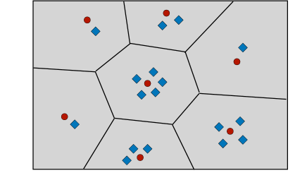
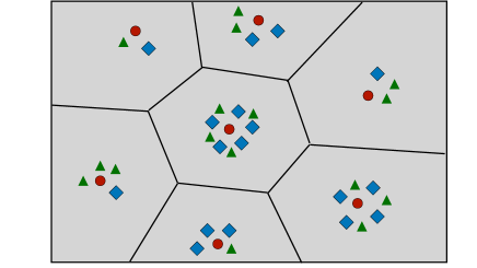
(a)	(b)

Figure 1: (a) Illustration of the Voronoi cells generated by the atoms of the true mixing measure $G_{0}$ (red points), and of the convergence rates of the fitted atoms of the (possibly penalized) MLE (blue points), under the pointwise setting. The cardinality of each Voronoi cell is the number of atoms of the MLE in these cells. The atoms and mixing weights of the MLE in the Voronoi cells with cardinality one have $n^{-1/2}$ convergence rates, where we ignore polylogarithmic factors. When the model is 2-strongly identifiable, the atoms of the MLE in the Voronoi cells with cardinality greater than one converge at the slow rate $n^{-1/4}$, while their mixing weights have $n^{-1/2}$ rates of convergence. Under location-scale Gaussian mixtures, the location and scale mixing components of the Voronoi cells with $l\geq 2$ elements respectively have convergence rates $n^{-1/2\bar{r}(l)}$ and $n^{-1/\bar{r}(l)}$ while their mixing weights have $n^{-1/2}$ rates of convergence. (b) Illustration of the Voronoi cells generated by the limiting mixing measure $G_{*}$ under the uniform setting of Section 4. The red, blue, and green points respectively denote the atoms of the limiting measure $G_{*}$, the penalized MLE $\widehat{G}_{n}$, and the varying true mixing measure $G_{0}^{n}$. The atoms in each Voronoi cell with $l\geq 2$ atoms of $\widehat{G}_{n}$ or $G_{0}^{n}$ converge at the rate $n^{-1/2(l-1)}$.

3.2 Weakly Identifiable Case: Location-Scale Gaussian Mixtures

In this section, we study the convergence rate of the MLE when the model is not strongly identifiable in the second order. Location-scale Gaussian mixtures are a popular example of such models, as a result of the following equation:

$$\frac{\partial^{2}{f}}{\partial{\mu}\partial\mu^{\top}}(x|\mu,\Sigma)=2\frac{\partial{f}}{\partial{\Sigma}}(x|\mu,\Sigma),$$ (5)

for all $x\in\mathbb{R}^{d}$ and $\theta=(\mu,\Sigma)\in\Theta$, where $\mathcal{F}=\{f(\cdot|\theta):\theta\in\Theta\}$ denotes the family of location-scale Gaussian densities, with compact parameter space $\Theta\subseteq\mathbb{R}^{d}\times\mathbb{S}^{d-1}$. The absence of second order identifiability in location-scale Gaussian mixtures leads to several challenges in studying the convergence rates of the MLE. To simplify our proofs, we will assume that all mixing measures have weights which are lower bounded by some small constant $c_{0}>0$. As a result, we only state a convergence rate for the penalized MLE $\widehat{G}_{n}$, which indeed lies in the class $\mathcal{O}_{k,c_{0}}(\Theta)$ with high probability, by Proposition 3. We would like to remark that constraints on the mixing weights are also assumed in past work on convergence rates for over-specified location-scale Gaussian mixtures (Ho and Nguyen, 2016a, ), and are not a byproduct of our choice of loss function.

Proposition 2.2 in Ho and Nguyen, 2016a , together with Theorem 2 and Proposition 3, may be used to establish the following bound, for some constant $C(G_{0})>0$,

$$\mathbb{E}\big{[}W_{\overline{r}(k-k_{0}+1)}(\widehat{G}_{n},G_{0})\big{]}\leq C(G_{0})\left(\frac{\log n}{\sqrt{n}}\right)^{\frac{1}{\overline{r}(k-k_{0}+1)}},$$

where for any $k^{\prime}\geq 2$, $\overline{r}(k^{\prime})$ is defined as the smallest integer $r$ such that the system of polynomial equations

$$\sum\limits_{j=1}^{k^{\prime}}\sum\limits_{n_{1},n_{2}}\dfrac{c_{j}^{2}a_{j}^{n_{1}}b_{j}^{n_{2}}}{n_{1}!n_{2}!}=0,\leavevmode\nobreak\ \leavevmode\nobreak\ \ \text{for each}\ \alpha=1,\ldots,r$$ (6)

does not have any nontrivial solution for the unknown variables $(a_{j},b_{j},c_{j})_{j=1}^{k^{\prime}}\subseteq\mathbb{R}$. The range of $(n_{1},n_{2})$ in the second sum consist of all natural pairs satisfying the equation $n_{1}+2n_{2}=\alpha$. A solution to the above system is considered nontrivial if all variables $c_{j}$ are non-zero, while at least one of the $a_{j}$ is non-zero. For example, it was shown by Ho and Nguyen, 2016b that $\bar{r}(2)=4$ and $\bar{r}(3)=6$.

The convergence rate $(\log n/\sqrt{n})^{1/\overline{r}(k-k_{0}+1)}$ of $\widehat{G}_{n}$ indicates that the location and scale parameters of the penalized MLE converge to their population counterparts at this same slow rate. As before, this result does not precisely reflect the behavior of individual parameters in location-scale Gaussian mixtures, leading us to consider a stronger loss function than the Wasserstein distance. Given $G=\sum_{i=1}^{k^{\prime}}p_{i}\delta_{(\mu_{i},\Sigma_{i})}\in\mathcal{E}_{k^{\prime}}(\Theta)$ for $k^{\prime}\leq k$, define the Voronoi cells $\mathcal{A}_{j}=\mathcal{A}_{j}(G)=\{i\in[k^{\prime}]:\|\mu_{i}-\mu_{j}^{0}\|+\|\Sigma_{i}-\Sigma_{j}^{0}\|\leq\|\mu_{i}-\mu_{\ell}^{0}\|+\|\Sigma_{i}-\Sigma_{\ell}^{0}\|\ \forall\ell\neq j\}$, for $j\in[k_{0}]$, and set

$$\macc@depth\char 1\relax\frozen@everymath{\macc@group}\macc@set@skewchar\macc@nested@a 111{}(G,G_{0}) :=\sum_{j:|\mathcal{A}_{j}|=1}\sum_{i\in\mathcal{A}_{j}}p_{i}\left(\|\mu_{i}-\mu_{j}^{0}\|+\|\Sigma_{i}-\Sigma_{j}^{0}\|\right)$$

$$+\sum_{j:|\mathcal{A}_{j}|>1}\sum_{i\in\mathcal{A}_{j}}p_{i}\left(\|\mu_{i}-\mu_{j}^{0}\|^{\bar{r}(|\mathcal{A}_{j}|)}+\|\Sigma_{i}-\Sigma_{j}^{0}\|^{\frac{\bar{r}(|\mathcal{A}_{j}|)}{2}}\right)+\sum_{j=1}^{k_{0}}\left|\sum_{i\in\mathcal{A}_{j}}p_{i}-p_{j}^{0}\right|.$$

It can be shown that $\macc@depth\char 1\relax\frozen@everymath{\macc@group}\macc@set@skewchar\macc@nested@a 111{}\gtrsim W_{\overline{r}(k-k_{0}+1)}^{{\macc@depth\char 1\relax\frozen@everymath{\macc@group}\macc@set@skewchar\macc@nested@a 111{r}(k-k_{0}+1)}}$ and

$$\sup_{\begin{subarray}{c}G\neq G_{0}\\ G\in\mathcal{O}_{k}(\Theta)\end{subarray}}\macc@depth\char 1\relax\frozen@everymath{\macc@group}\macc@set@skewchar\macc@nested@a 111{}(G,G_{0})/W_{\overline{r}(k-k_{0}+1)}^{{\macc@depth\char 1\relax\frozen@everymath{\macc@group}\macc@set@skewchar\macc@nested@a 111{r}(k-k_{0}+1)}}(G,G_{0})=\infty.$$

The proof is similar to that of Lemma 14 in Appendix B; therefore, it is omitted. We deduce that $\macc@depth\char 1\relax\frozen@everymath{\macc@group}\macc@set@skewchar\macc@nested@a 111{}$ is a stronger loss function than $W_{\overline{r}(k-k_{0}+1)}^{{\overline{r}(k-k_{0}+1)}}$. We bound the risk of the penalized MLE under $\macc@depth\char 1\relax\frozen@everymath{\macc@group}\macc@set@skewchar\macc@nested@a 111{}$ as follows.

Theorem 5.

Let $\mathcal{F}$ denote the location-scale Gaussian density family with parameter space taking the form $\Theta=[-a,a]^{d}\times\Omega$, where $a>0$ and $\Omega$ is a compact subset of $\leavevmode\nobreak\ \mathbb{S}^{d-1}$ whose eigenvalues lie in a closed interval contained in $(0,\infty)$. Then, there exists a constant $C(G_{0})>0$, depending only on $G_{0},k,d,\Theta$, such that

$$\mathbb{E}\left[\macc@depth\char 1\relax\frozen@everymath{\macc@group}\macc@set@skewchar\macc@nested@a 111{}(\widehat{G}_{n},G_{0})\right]\leq C(G_{0})\frac{\log n}{\sqrt{n}}.$$

The proof of Theorem 5 appears in Appendix A.4. Recall that $\widehat{G}_{n}=\sum_{i=1}^{\widehat{k}_{n}}\widehat{p}_{i}^{n}\delta_{(\widehat{\mu}_{i}^{n},\widehat{\Sigma}_{i}^{n})}$, and write $\mathcal{A}_{j}^{n}=\mathcal{A}_{j}(\widehat{G}_{n})$ for all $j\in[k_{0}]$. Theorem 5 implies the following.

1. Given $j\in[k_{0}]$ such that $|\mathcal{A}_{j}^{n}|\geq 2$, we have, with probability tending to one,

   $$\|\widehat{\mu}_{i}^{n}-\mu_{j}^{0}\| \lesssim(\log n/\sqrt{n})^{1/\bar{r}(|\mathcal{A}_{j}^{n}|)},\quad\text{and,}\quad\|\widehat{\Sigma}_{i}^{n}-\Sigma_{j}^{0}\|\lesssim(\log n/\sqrt{n})^{2/\bar{r}(|\mathcal{A}_{j}^{n}|)},\leavevmode\nobreak\ \leavevmode\nobreak\ i\in\mathcal{A}_{j}^{n}.$$

   In particular, the location parameters of $\widehat{G}_{n}$ converge quadratically slower than the scale parameters.

2. On the other hand, for any index $j\in[k_{0}]$ such that $|\mathcal{A}_{j}^{n}|=1$ and for any $i\in\mathcal{A}_{j}^{n}$, we have with probability tending to one,

   $$\|\widehat{\mu}_{i}^{n}-\mu_{j}^{0}\|\vee\|\widehat{\Sigma}_{i}^{n}-\Sigma_{j}^{0}\|\lesssim\log n/\sqrt{n}.$$ (7)

   Hence, both location and scale parameters of $\widehat{G}_{n}$ achieve the standard parametric rate up to a logarithmic factor. We refer to Figure 1(a) for an illustration of these convergence rates.

3. Notice that $|\mathcal{A}_{j}^{n}|\leq\widehat{k}_{n}-k_{0}+1$ for all $j\in[k_{0}]$. When equality is achieved for some $j$, there must be a single Voronoi cell with $\widehat{k}_{n}-k_{0}+1$ elements, while the remaining cells each have exactly one component. In this case, there are $k_{0}-1$ components of the penalized MLE which achieve the fast pointwise rate (7).

4. When $k=k_{0}+1$, there exists a unique index $j$ such that $\mathcal{A}_{j}^{n}$ has at most two components, while the remaining Voronoi cells have exactly one component. Since $\overline{r}(2)=4$, this demonstrates that the two components having indices in $\mathcal{A}_{j}$ have means converging at the slow rate $n^{-1/8}$, and covariances converging at the rate $n^{-1/4}$, up to polylogarithmic factors. These particular rates were already anticipated by the work of Chen and Chen, (2003) when $k_{0}=1$. When $k_{0}>1$, our work shows that the remaining $k_{0}-1$ atoms of the penalized MLE converge at the fast rate (7).

5. When $k=k_{0}+2$, there are two possible cases: either (a) there exists a unique index $j^{\prime}$ such that $\mathcal{A}_{j^{\prime}}^{n}$ has at most three components while the remaining sets have exactly one component, or (b) there exist indices $j^{\prime}_{1}$ and $j_{2}^{\prime}$ such that $\mathcal{A}_{j_{1}^{\prime}}^{n}$ and $\mathcal{A}_{j_{2}^{\prime}}^{n}$ have at most two components while the remaining sets have exactly one component. Under case (a), since $\overline{r}(3)=6$, the means with indices in $\mathcal{A}_{j^{\prime}}^{n}$ converge at the rate $(\log n/n)^{1/12}$ while the remaining atoms of $\widehat{G}_{n}$ converge at the parametric rate. Under case (b), the means with indices in $\mathcal{A}_{j_{1}^{\prime}}^{n}\cup\mathcal{A}_{j_{2}^{\prime}}^{n}$ converge at the $(\log n/n)^{1/8}$ rate while the remaining atoms converge at the rate $(\log n/n)^{1/2}$.

Finally, similarly to the loss function $\mathcal{D}$ in equation (3), we note that $\macc@depth\char 1\relax\frozen@everymath{\macc@group}\macc@set@skewchar\macc@nested@a 111{}(G,G_{0})$ can be computed in $O(k\times k_{0})$ time for any given $G\in\mathcal{O}_{k}(\Theta)$, and thus enjoys a computational advantage over the Wasserstein metric.

4 Uniform Convergence Rates of the MLE

Thus far, we have derived pointwise convergence rates for the MLE or penalized MLE, which depend on the fixed mixing measure $G_{0}$. We next consider uniform rates of convergence, in which we allow the true mixing measure $G_{0}\equiv G_{0}^{n}\in\mathcal{E}_{k_{0}}(\Theta)$ to vary with the sample size $n$, while converging to some limiting mixing measure $G_{*}=\sum_{i=1}^{k_{*}}p_{i}^{*}\delta_{\theta_{i}^{*}}\in\mathcal{E}_{k_{*}}(\Theta)$, of order $k_{*}\leq k_{0}\leq k$. To simplify our proofs, we will assume throughout this section that $\Theta\subseteq\mathbb{R}$.

It is known that the optimal pointwise rate of estimation in a strongly identifiable mixture differs from the optimal uniform rate. Indeed, when $\mathcal{F}$ is $(k+k_{0})$-strongly identifiable it can be inferred from Theorem 6.3 in (Heinrich and Kahn,, 2018) that,

$$\mathbb{E}\big{[}W_{r}(\macc@depth\char 1\relax\frozen@everymath{\macc@group}\macc@set@skewchar\macc@nested@a 111{G}_{n},G_{0}^{n})\big{]}\lesssim\left(\frac{\log n}{n}\right)^{1/2r},$$ (8)

where we fix $r=k+k_{0}-2k_{*}+1$ throughout the remainder of this section. Furthermore, the above rate is minimax optimal up to a polylogarithmic factor, but is markedly slower than its pointwise analogue discussed in Section 3.1. It implies that the atoms of $\macc@depth\char 1\relax\frozen@everymath{\macc@group}\macc@set@skewchar\macc@nested@a 111{G}_{n}$ with nonvanishing weights tend to those of $G_{0}^{n}$ at this same slow rate. In contrast, we will show that the uniform convergence rates of individual components of the MLE can be sharpened. Similarly to the previous subsection, however, our results will rely on the additional condition that the mixing proportions of $G_{0}^{n},G_{*}$ are uniformly bounded below by a small constant $c_{0}>0$. While this condition was not needed in the work of Heinrich and Kahn, (2018), we require it for our proof technique. As a result, we focus on deriving convergence rates for the penalized MLE $\widehat{G}_{n}$.

Given $k^{\prime}\in[k]$, let $G=\sum_{i=1}^{k^{\prime}}p_{i}\delta_{\theta_{i}}\in\mathcal{E}_{k^{\prime}}(\Theta)$ and $G^{\prime}=\sum_{i=1}^{k_{0}}p_{i}^{\prime}\delta_{\theta_{i}^{\prime}}\in\mathcal{E}_{k_{0}}(\Theta)$. We again partition the supports of these measures into Voronoi cells, which are now generated by the atoms of the measure $G_{*}$ rather than $G_{0}^{n}$:

$$\mathcal{A}_{j}(G)=\big{\{}i\in[k^{\prime}]:|\theta_{i}-\theta_{j}^{*}|\leq|\theta_{i}-\theta_{\ell}^{*}|\ \forall\ell\neq j\big{\}},$$

for all $j\in[k_{*}]$. With this notation in place, we define the following loss function over $\mathcal{O}_{k}(\Theta)$,

$$\widetilde{W}(G,G^{\prime})=\inf_{\boldsymbol{q}\in\Pi(G,G^{\prime})}\left\{\sum_{l=1}^{k_{*}}\sum_{(i,j)\in\mathcal{A}_{l}(G)\times\mathcal{A}_{l}(G^{\prime})}q_{ij}|\theta_{i}-\theta_{j}^{\prime}|^{|\mathcal{A}_{l}(G)|+|\mathcal{A}_{l}(G^{\prime})|-1}+\sum_{(i,j)\not\in\cup_{l=1}^{k_{*}}\mathcal{A}_{l}(G)\times\mathcal{A}_{l}(G^{\prime})}q_{ij}\right\}.$$ (9)

$\widetilde{W}$ may be viewed as a generalized optimal transport cost, whose ground cost depends on the measures $G,G^{\prime}$ via the exponent $|\mathcal{A}_{l}(G)|+|\mathcal{A}_{l}(G^{\prime})|-1$. In the special case where $k_{*}=1$, this exponent is given by $k+k_{0}-1$, and $\widetilde{W}$ is then equal to $W_{r}^{r}$. On the other hand, when $k_{*}>1$, it can be seen similarly as in previous subsections that,

$$\widetilde{W}\gtrsim W_{r}^{r},\leavevmode\nobreak\ \leavevmode\nobreak\ \text{and }\leavevmode\nobreak\ \sup_{\begin{subarray}{c}G\neq G^{\prime}\end{subarray}}\frac{\widetilde{W}(G,G^{\prime})}{W_{r}^{r}(G,G^{\prime})}=\infty.$$ (10)

Therefore, the loss function $\widetilde{W}$ is stronger than the Wasserstein distances used by Heinrich and Kahn, (2018). The main result of this section is the following convergence rate under $\widetilde{W}$.

Theorem 6.

Let $k\geq k_{0}\geq k_{*}$ and $c_{0}>0$. Assume that $G_{*}\in\mathcal{E}_{k_{*},c_{0}}(\Theta)$ and $G_{0}^{n}\in\mathcal{E}_{k_{0},c_{0}}(\Theta)$ for all $n\geq 1$. Furthermore, assume that $\mathcal{F}$ is $(k+k_{0})$-strongly identifiable, and satisfies conditions A($k+k_{0}$) and B($k$). Then, there exist constants $C,\epsilon>0$, depending only on $\mathcal{F},k,c_{0}$, such that for all $n\geq 1$ satisfying $\widetilde{W}(G_{0}^{n},G_{*})\leq\epsilon$, we have

$$\mathbb{E}\Big{[}\widetilde{W}(\widehat{G}_{n},G_{0}^{n})\Big{]}\leq C\frac{\log n}{\sqrt{n}}.$$

In view of equation (10) and the existing minimax lower bound of Heinrich and Kahn, (2018) under the Wasserstein distance, it can immediately be deduced that the convergence rate in Theorem 6 is minimax optimal, up to a logarithmic factor.

The proof of Theorem 6 appears in Appendix A.5. Our main technical contribution is Lemma 11 therein, which provides an upper bound on $\widetilde{W}(G,G_{0})$ in terms of the Kolmogorov-Smirnov distance between the distributions of $p_{G}$ and $p_{G_{0}}$. Similarly to Heinrich and Kahn, (2018), we derive our upper bound by placing the atoms of $G$ and $G_{0}$ into an ultrametric tree, and using it to construct a nearly optimal coupling $\mathbf{q}$ in the definition of $\widetilde{W}$. These derivations are facilitated by the assumption $\Theta\subseteq\mathbb{R}$, but we expect that similar conclusions also hold for strongly identifiable families with multidimensional parameter spaces.

Theorem 6 may be interpreted similarly as in previous sections, thus we only provide an example. In the sequel, we ignore polylogarithmic factors. For all $l\in[k_{*}]$, notice that

$$|\mathcal{A}_{l}(\widehat{G}_{n})|\leq k-k_{*}+1,\quad|A_{l}(G_{0}^{n})|\leq k_{0}-k_{*}+1.$$ (11)

When these inequalities are both achieved by the same index $\bar{l}\in[k_{*}]$, we find that for every $i\in\mathcal{A}_{\bar{l}}(\widehat{G}_{n})$, there exists $j\in\mathcal{A}_{\bar{l}}(G_{0}^{n})$ such that, up to taking subsequences, the rate of Heinrich and Kahn, (2018) is achieved:

$$|\widehat{\theta}_{i}^{n}-\theta_{j}^{0}|\lesssim n^{-\frac{1}{2r}}.$$

However, the remaining $k_{*}-1$ atoms of the penalized MLE converge uniformly at the parametric rate $n^{-1/2}$, which could not have been deduced from equation (8). Furthermore, we emphasize that this setting—in which all redundant atoms of $\widehat{G}_{n}$ and $G_{0}^{n}$ are concentrated near a single atom of $G_{*}$—is the only case where a subset of the atoms of $\widehat{G}_{n}$ achieve the worst-case rate predicted by Heinrich and Kahn, (2018). Indeed, when the inequalities (11) are strict, rates faster than $n^{-1/2r}$ are achieved by all atoms of $\widehat{G}_{n}$.

5 Discussion

The aim of our work has been to sharpen known convergence rates of the MLE for estimating individual parameters of a finite mixture model. Our key observation was that the Wasserstein distance, despite being an elegant tool for metrizing the space of mixing measures, is not well-suited to capturing the heterogeneous convergence behaviour of individual mixture parameters. We instead proposed new loss functions which achieve this goal. Our theoretical results are supported by a simulation study, which is deferred to Appendix C.

Our analysis has focused on maximum likelihood-based estimators, whose computation involves the nonconvex optimization problem (1). Despite significant recent advances in the theoretical understanding of the EM algorithm for approximating the MLE in finite mixtures (Balakrishnan et al.,, 2017; Dwivedi et al., 2020b, ; Kwon et al.,, 2019; Dwivedi et al., 2020a, ), we make no claims that such approximations obey the asymptotics described in this paper, leaving open a potential gap between theory and practice. The method of moments provides a practical alternative to the MLE, which is minimax optimal for certain classes of finite mixture models under the Wasserstein distance (Wu and Yang,, 2020; Doss et al.,, 2020). We leave open the question of characterizing the risk of moment-based estimators under the loss functions proposed in our work.

In Section 4, we obtained uniform convergence rates for strongly identifiable mixtures with mixing proportions bounded away from zero. We leave open the question of determining whether this constraint can be removed.

Finally, we derived both pointwise and uniform convergence rates for strongly identifiable mixtures, however we restricted our analysis of location-scale Gaussian mixtures to the pointwise case. Obtaining uniform convergence rates for such models remains an important open problem, which has not been studied beyond the special case of two component models (Hardt and Price,, 2015; Manole and Ho,, 2020). While this setting is beyond the scope of our work, we expect that considerations about the heterogeneity of parameter estimation, similar to those studied in this paper, would arise in such models as well.

Acknowledgements

TM was supported in part by the Natural Sciences and Engineering Research Council of Canada, through a PGS D scholarship. NH gratefully acknowledges research gifts by UT Austin ML grant.

Supplement to “Refined Convergence Rates for Maximum Likelihood Estimation under Finite Mixture Models”

In this supplementary material, we provide all proofs of results stated in the main text (Appendix A). We also state and prove certain results which were deferred from the main text (Appendix B), and provide a simulation study to illustrate the various convergence rates that were derived in this paper (Appendix C).

Appendix A Proofs

A.1 Proof of Theorem 2

Theorem 2(i) is an immediate consequence of Theorem 7.4 of van de Geer, (2000), which provides a generic exponential inequality for the Hellinger loss of nonparametric maximum likelihood density estimators, under mere conditions on the bracketing integral $\mathcal{J}_{B}(\epsilon,\macc@depth\char 1\relax\frozen@everymath{\macc@group}\macc@set@skewchar\macc@nested@a 111{}_{k}^{1/2}(\Theta,\epsilon),\nu)$. The application of this result to finite mixture models has previously been discussed by Ho and Nguyen, 2016b ; Ho and Nguyen, 2016a .

Theorem 2(ii) also follows by the same proof technique as Theorem 7.4 of van de Geer, (2000), with modifications to account for the presence of the penalty in the definition of $\widehat{G}_{n}$. An analogue of this result was previously proven by Manole and Khalili, (2021), though with different conditions on the tuning parameter $\xi_{n}$. For completeness, we provide a self-contained proof of Theorem 2(ii), under the conditions on $\xi_{n}$ required for our development.

As in van de Geer, (2000), we shall reduce the problem to controlling the increments of the empirical process

$$\nu_{n}(G)=\sqrt{n}\int_{\{p_{G_{0}}>0\}}\frac{1}{2}\log\frac{\bar{p}_{G}}{p_{G_{0}}}\leavevmode\nobreak\ d(P_{n}-P_{G_{0}}),$$

where we recall that $\bar{p}_{G}=(p_{G}+p_{G_{0}})/2$, and we denote by $P_{G}=\int p_{G}d\nu$ the distribution induced by $p_{G}$, for any $G\in\mathcal{O}_{k}(\Theta)$. Furthermore, $P_{n}=(1/n)\sum_{i=1}^{n}\delta_{X_{i}}$ denotes the empirical measure. Our main technical tool will be the following special case of Theorem 5.11 (van de Geer, (2000); see also Lemma 7.2–7.3 therein).

Theorem 7 (Theorem 5.11 (van de Geer,, 2000)).

Let $R>0$ and $k\geq 1$. Given $\mathcal{G}\subseteq\mathcal{O}_{k}(\Theta)$, let $G_{0}\in\mathcal{G}$. Furthermore, given a universal constant $C>0$, let $a,C_{1}>0$ be chosen such that

$$a\leq C_{1}\sqrt{n}R^{2}\wedge 8\sqrt{n}R,$$ (12)

and,

$$a\geq\sqrt{C^{2}(C_{1}+1)}\left(\int_{0}^{R}\sqrt{H_{B}\left(\frac{u}{\sqrt{2}},\Big{\{}p_{G}:G\in\mathcal{G},h(\bar{p}_{G},p_{0})\leq R\Big{\}},\nu\right)}du\vee R\right),$$ (13)

Then,

$$\mathbb{P}\left\{\sup_{\begin{subarray}{c}G\in\mathcal{G}\\ h(\bar{p}_{G},p_{G_{0}})\leq R\end{subarray}}|\nu_{n}(G)|\geq a\right\}\leq C\exp\left(-\frac{a^{2}}{C^{2}(C_{1}+1)R^{2}}\right).$$

We are now in a position to prove the claim.

Proof of Theorem 2(ii). Let $G_{0}\in\mathcal{O}_{k,c_{0}}(\Theta)$. By a straightforward modification of Lemma 4.1 of van de Geer, (2000), we have

$$h^{2}\left(\bar{p}_{\widehat{G}_{n}},p_{G_{0}}\right)\leq\frac{1}{\sqrt{n}}\nu_{n}(\widehat{G}_{n})+\frac{\xi_{n}\rho(G_{0})}{4n}.$$ (14)

Let $u>\gamma_{n}=L\log n/\sqrt{n}$, where $L$ is the constant in assumption B($k$). In view of equation (14), and the fact that $h^{2}(p_{G},p_{G_{0}})\leq 4h(\bar{p}_{G},p_{G_{0}})$ for all $G\in\mathcal{O}_{k}(\Theta)$ (cf. Lemma 4.2 of van de Geer, (2000)), we have

$$\mathbb{P}\left\{h(p_{\widehat{G}_{n}},p_{G_{0}})>u\right\}\leq\mathbb{P}\left\{h(\bar{p}_{\widehat{G}_{n}},p_{G_{0}})>u/4\right\}$$

$$\leq\mathbb{P}\left\{\sup_{\begin{subarray}{c}G\in\mathcal{O}_{k,c_{0}}(\Theta)\\ h(\bar{p}_{G},p_{0})>u/4\end{subarray}}n^{-\frac{1}{2}}\nu_{n}(G)+\frac{\xi_{n}\rho(G_{0})}{4n}-h^{2}(\bar{p}_{G},p_{G_{0}})\geq 0\right\}.$$

Let $\mathcal{S}=\min\{s:2^{s+1}u/4>1\}$. Then,

$$\mathbb{P}\Bigg{\{}\sup_{\begin{subarray}{c}G\in\mathcal{O}_{k,c_{0}}(\Theta)\\ h(\bar{p}_{G},p_{G_{0}})>u/4\end{subarray}} n^{-\frac{1}{2}}\nu_{n}(G)+\frac{\xi_{n}\rho(G_{0})}{4n}-h^{2}(\bar{p}_{G},p_{0})\geq 0\Bigg{\}}$$

$$\leq\sum_{s=0}^{\mathcal{S}}\mathbb{P}\left\{\sup_{\begin{subarray}{c}G\in\mathcal{O}_{k,c_{0}}(\Theta)\\ h(\bar{p}_{G},p_{G_{0}})\leq(2^{s+1})u/4\end{subarray}}\nu_{n}(G)\geq\sqrt{n}2^{2s}\left(\frac{u}{4}\right)^{2}-\frac{\xi_{n}\rho(G_{0})}{4\sqrt{n}}\right\}.$$

We have thus reduced the problem to that of bounding the supremum of the empirical process $\nu_{n}$, for which we shall invoke Theorem 7. Let $R=2^{s+1}u$, $C_{1}=15$, and

$$a=\sqrt{n}2^{2s}\left(\frac{u}{4}\right)^{2}-\frac{\xi_{n}\rho(G_{0})}{4\sqrt{n}}.$$

It can be directly verified that condition (12) holds for all $s=0,\dots,\mathcal{S}$. To further show that condition (13) holds, note that

$$\int_{0}^{2^{s+1}u}\sqrt{H_{B}\left(\frac{t}{\sqrt{2}},\macc@depth\char 1\relax\frozen@everymath{\macc@group}\macc@set@skewchar\macc@nested@a 111{}_{k}^{1/2}\left(\Theta,2^{s+1}\frac{t}{4}\right),\nu\right)}dt\vee 2^{s+1}u$$

$$\leq\sqrt{2}\int_{0}^{2^{s+\frac{1}{2}}u}\sqrt{H_{B}\left(t,\macc@depth\char 1\relax\frozen@everymath{\macc@group}\macc@set@skewchar\macc@nested@a 111{}_{k}^{1/2}\left(\Theta,2^{s+\frac{1}{2}}t\right),\nu\right)}dt\vee 2^{s+1}u$$

$$\leq 2\mathcal{J}_{B}\left(2^{s+1}u,\macc@depth\char 1\relax\frozen@everymath{\macc@group}\macc@set@skewchar\macc@nested@a 111{}_{k}^{1/2}(\Theta,2^{s+1}u),\nu\right)\leq 2J\sqrt{n}2^{2s+1}u^{2},$$

where we invoked condition B($k$). Now, notice that $\rho(G_{0})$ is bounded above by a universal constant $L_{0}>0$ depending only on $k,c_{0}$, irrespective of the choice of $G_{0}\in\mathcal{O}_{k,c_{0}}(\Theta)$. Furthermore, we have $\sqrt{n}\gamma_{n}^{2}\asymp(\log n)^{2}/\sqrt{n}$, and $\xi_{n}/\sqrt{n}\asymp\log n/\sqrt{n}$, thus for all $u>\gamma_{n}$, the second term in the definition of $a$ is of lower order than the first. Deduce that there exists a constant $N>0$, depending only on $L_{0},c_{1},k$ such that for all $n\geq N$,

$$a\geq\frac{1}{2}\sqrt{n}2^{2s}(u/4)^{2}=\sqrt{n}2^{2s-5}u^{2}\geq\sqrt{C_{0}}\cdot\big{(}2J\sqrt{n}2^{2s+1}u^{2}\big{)},$$

for a sufficiently small choice of the universal constant $J>0$. We may therefore invoke Theorem 7, to deduce that for all $n\geq N$,

$$\mathbb{P}\left\{h(p_{\widehat{G}_{n}},p_{G_{0}})>u\right\} \leq\sum_{s=0}^{\mathcal{S}}\mathbb{P}\left\{\sup_{\begin{subarray}{c}\mathcal{O}_{k,c_{0}}(\Theta)\\ h(\bar{p}_{G},p_{G_{0}})\leq(2^{s+1})u/4\end{subarray}}\nu_{n}(G)\geq\sqrt{n}2^{2s-5}u^{2}\right\}$$

$$\leq C\sum_{s=0}^{\infty}\exp\left\{-\frac{1}{16C^{2}2^{2s+2}\gamma_{n}^{2}}\left[\sqrt{n}2^{2s-5}u^{2}\right]^{2}\right\}$$

$$\leq C\sum_{s=0}^{\infty}\exp\left\{\frac{n2^{2s-16}u^{2}}{C^{2}}\right\}$$

$$\leq c\exp(-nu^{2}/c),$$

for a large enough constant $c>0$. It follows that, for all $n\geq N$,

$$\mathbb{E}h(p_{\widehat{G}_{n}},p_{G_{0}})=\int_{0}^{\infty}\mathbb{P}(h(p_{\widehat{G}_{n}},p_{G_{0}})\geq u)du\leq\gamma_{n}+c\int_{\gamma_{n}}^{\infty}\exp\left\{-\frac{nu^{2}}{c}\right\}du\leq c^{\prime}\gamma_{n},$$

for another universal constant $c^{\prime}>0$. Since the Hellinger distance is bounded above by 1, it is clear that the above display holds for all $n\geq 1$, up to modifying the constant $c^{\prime}$ in terms of $N$. Furthermore, the above calculation is clearly uniform in the $G_{0}$ under consideration, so the claim follows. ∎

A.2 Proof of Proposition 3

We shall require a bound on the log-likelihood ratio statistic based on the MLE $\macc@depth\char 1\relax\frozen@everymath{\macc@group}\macc@set@skewchar\macc@nested@a 111{G}_{n}$. Such a bound is implicit in the proof of Theorem 7.4 of van de Geer, (2000). Specifically, the following can be deduced from their Corollary 7.5.

Proposition 8 (Corollary 7.5 van de Geer, (2000)).

Assume that condition B($k$) holds. Then, given $k\geq 1$, there exists a constant $C>0$ depending on $k,d$ and $\mathcal{F}$, such that for all $u\geq L(\log n/n)^{1/2}$,

$$\sup_{G_{0}\in\mathcal{O}_{k}(\Theta)}\mathbb{P}_{G_{0}}\left(\int\log\frac{p_{\macc@depth\char 1\relax\frozen@everymath{\macc@group}\macc@set@skewchar\macc@nested@a 111{G}_{n}}}{p_{G_{0}}}dP_{n}\geq u^{2}\right)\leq C\exp\left(-\frac{nu^{2}}{C^{2}}\right).$$

Let $G_{0}\in\mathcal{O}_{k,c_{0}}(\Theta)$. After possibly replacing $C$ by $C\vee L$, apply Proposition 8 with $u=C\sqrt{\log n/n}$ to deduce that

$$\ell_{n}(\macc@depth\char 1\relax\frozen@everymath{\macc@group}\macc@set@skewchar\macc@nested@a 111{G}_{n})-\ell_{n}(G_{0})\leq C^{2}\log n,$$

with probability at least $1-C/n$. Now, by definition of the penalized MLE $\widehat{G}_{n}$ and of the non-penalized MLE $\macc@depth\char 1\relax\frozen@everymath{\macc@group}\macc@set@skewchar\macc@nested@a 111{G}_{n}$, we have

$$0\leq\Big{[}\ell_{n}(\widehat{G}_{n})-\ell_{n}(G_{0})\Big{]}+\xi_{n}\left[\rho(\widehat{G}_{n})-\rho(G_{0})\right] \leq\Big{[}\ell_{n}(\macc@depth\char 1\relax\frozen@everymath{\macc@group}\macc@set@skewchar\macc@nested@a 111{G}_{n})-\ell_{n}(G_{0})\Big{]}+\xi_{n}\left[\rho(\widehat{G}_{n})-\rho(G_{0})\right]$$

$$\leq C^{2}\log n+\xi_{n}\left[\rho(\widehat{G}_{n})-\rho(G_{0})\right],$$

with probability at least $1-C/n$. Therefore, since $\xi_{n}\geq\log n$, we obtain

$$\rho(\widehat{G}_{n})\geq-C^{2}+\rho(G_{0})\geq-C^{2}+k_{0}\log c_{0}=-C_{1},$$

where $C_{1}=C^{2}+k_{0}\log(1/c_{0})>0$. By definition of $\rho$, it must follow that

$$\widehat{p}_{i}^{n}\geq\exp(-C_{1}),\quad i=1,\dots,\widehat{k}_{n},$$

with probability at least $1-C/n$. The claim follows with $c=\exp(C_{1})\vee C$. ∎

A.3 Proof of Theorem 4

The claim will follow from the following result, relating the discrepancy $\mathcal{D}(G,G_{0})$ to the Total Variation distance between the corresponding densities $p_{G}$ and $p_{G_{0}}$.

Lemma 9.

Assume the same conditions as Theorem 4. Then, there exists a constant $c>0$ depending on $G_{0},d,k,\mathcal{F}$, such that for any $G\in\mathcal{O}_{k}(\Theta)$,

$$V(p_{G},p_{G_{0}})\geq c\mathcal{D}(G,G_{0}).$$ (15)

Recall that we have assumed condition B($k$). Therefore, by combining Lemma 9 with Theorem 2(i) and the well-known inequality $V\leq h$, we deduce that

$$\mathbb{E}\mathcal{D}(\macc@depth\char 1\relax\frozen@everymath{\macc@group}\macc@set@skewchar\macc@nested@a 111{G}_{n},G_{0})\lesssim\mathbb{E}V(p_{\macc@depth\char 1\relax\frozen@everymath{\macc@group}\macc@set@skewchar\macc@nested@a 111{G}_{n}},p_{G_{0}})\leq\mathbb{E}h(p_{\macc@depth\char 1\relax\frozen@everymath{\macc@group}\macc@set@skewchar\macc@nested@a 111{G}_{n}},p_{G_{0}})\lesssim\sqrt{\frac{\log n}{n}},$$

as claimed. It thus remains to prove Lemma 9.

Proof of Lemma 9.

Our proof proceeds using a similar argument as that of Ho and Nguyen, 2016b , though with key differences to account for our choice of loss function. We will prove that

$$\lim_{\delta\to 0}\inf_{\begin{subarray}{c}G\in\mathcal{O}_{k}(\Theta)\\ \mathcal{D}(G,G_{0})\leq\delta\end{subarray}}\frac{V(p_{G},p_{G_{0}})}{\mathcal{D}(G,G_{0})}>0.$$ (16)

This implies a local version of the claim, namely that there exist constants $\delta_{0},C>0$ such that for all $G\in\mathcal{O}_{k}(\Theta)$ satisfying $\mathcal{D}(G,G_{0})\leq\delta$,

$$\mathcal{D}(G,G_{0})\leq CV(p_{G},p_{G_{0}}).$$ (17)

We begin by showing how this local inequality leads to the claim, and we will then prove equation (16). Taking equation (16) for granted, it suffices to prove

$$\inf_{\begin{subarray}{c}G\in\mathcal{O}_{k}(\Theta)\\ \mathcal{D}(G,G_{0})\geq\delta_{0}\end{subarray}}\frac{V(p_{G},p_{G_{0}})}{\mathcal{D}(G,G_{0})}>0.$$ (18)

Suppose by way of a contradiction that the above display does not hold. Then, there exists a sequence of mixing measures $G_{n}\in\mathcal{O}_{k}(\Theta)$ with $\mathcal{D}(G_{n},G_{0})\geq\delta_{0}$ such that $\frac{V(p_{G_{n}},p_{G_{0}})}{\mathcal{D}(G_{n},G_{0})}\to 0.$ Since the parametric family $\mathcal{F}$ is assumed to be 2-strongly identifiable, the model $\{p_{G}:G\in\mathcal{O}_{k}(\Theta)\}$ is identifiable, thus the map

$$(G,G^{\prime})\in\mathcal{O}_{k}(\Theta)\times\mathcal{O}_{k}(\Theta)\mapsto V(p_{G},p_{G^{\prime}})$$

defines a metric on $\mathcal{O}_{k}(\Theta)$. Since this metric is bounded, the sequence $\{G_{n}\}$ admits a subsequence converging to some mixing measure $\macc@depth\char 1\relax\frozen@everymath{\macc@group}\macc@set@skewchar\macc@nested@a 111{G}\in\mathcal{O}_{k}(\Theta)$. For ease of exposition, we replace this subsequence by the entire sequence $G_{n}$ in what follows, thus we have $V(p_{G_{n}},p_{\macc@depth\char 1\relax\frozen@everymath{\macc@group}\macc@set@skewchar\macc@nested@a 111{G}})\to 0$. Now, notice that $\mathcal{D}(\macc@depth\char 1\relax\frozen@everymath{\macc@group}\macc@set@skewchar\macc@nested@a 111{G},G_{0})\geq\delta_{0}$ by definition of $G_{n}$. Furthermore, $V(p_{G_{n}},p_{G_{0}})\to 0$ by assumption. Combining these facts leads to $V(p_{G_{0}},p_{\macc@depth\char 1\relax\frozen@everymath{\macc@group}\macc@set@skewchar\macc@nested@a 111{G}})=0$, and hence $\macc@depth\char 1\relax\frozen@everymath{\macc@group}\macc@set@skewchar\macc@nested@a 111{G}=G_{0}$, which contradicts the fact that $\mathcal{D}(\macc@depth\char 1\relax\frozen@everymath{\macc@group}\macc@set@skewchar\macc@nested@a 111{G},G_{0})>0$, and hence proves equation (18).

It remains to prove the local inequality (16). We again assume by way of a contradiction that there exists a sequence of mixing measures $G_{n}=\sum_{i=1}^{k_{n}}p_{i}^{n}\delta_{\theta_{i}^{n}}\in\mathcal{O}_{k}(\Theta)$ such that $\mathcal{D}(G_{n},G_{0})\to 0$ but

$$\frac{V(p_{G_{n}},p_{G_{0}})}{\mathcal{D}(G_{n},G_{0})}\to 0,\quad n\to\infty.$$ (19)

Define

$$\mathcal{A}_{j}^{n}=\mathcal{A}_{j}(G_{n})=\{i\in\{1,\ldots,k_{n}\}:\|\theta_{i}^{n}-\theta_{j}^{0}\|\leq\|\theta_{i}^{n}-\theta_{\ell}^{0}\|\ \forall\ell\neq j\},\quad j=1,\dots,k_{0}.$$

Since $k_{n}\leq k$ for all $n$, there exists a subsequence of $G_{n}$ such that $k_{n}$ does not change with $n$. Therefore, up to replacing $G_{n}$ by this subsequence, we may assume that $k_{n}=k^{\prime}\leq k$ for all $n$. Similarly, since there are only a finite number of distinct sets $\mathcal{A}_{1}^{n}\times\ldots\times\mathcal{A}_{k_{0}}^{n}$ over the range of $n\geq 1$, we may assume without loss of generality that $\mathcal{A}_{j}=\mathcal{A}_{j}^{n}$ does not change with $n$, for all $j=1,\dots,k_{0}$. Now, consider the decomposition

$$p_{G_{n}}(x)-p_{G_{0}}(x) =\sum_{j:|\mathcal{A}_{j}|>1}\sum_{i\in\mathcal{A}_{j}}p_{i}\Big{(}f(x|\theta_{i}^{n})-f(x|\theta_{j}^{0})\Big{)}$$

$$+\sum_{j:|\mathcal{A}_{j}|=1}\sum_{i\in\mathcal{A}_{j}}p_{i}\Big{(}f(x|\theta_{i}^{n})-f(x|\theta_{j}^{0})\Big{)}+\sum_{j=1}^{k_{0}}(\bar{p}_{j}^{n}-p_{j}^{0})f(x|\theta_{j}^{0})$$

$$:=A_{n,1}(x)+A_{n,2}(x)+B_{n}(x),$$

where we write $\bar{p}_{j}^{n}=\sum_{i\in\mathcal{A}_{j}}p_{i}^{n}$ for all $j\in[k_{0}]$. By a Taylor expansion to second order, notice that

$$A_{n,1}(x)=\sum_{j:|\mathcal{A}_{j}|>1}\sum_{i\in\mathcal{A}_{j}}p_{i}\left[(\theta_{i}^{n}-\theta_{j}^{0})^{\top}\frac{\partial f}{\partial\theta}(x|\theta_{j}^{0})+\frac{1}{2}(\theta_{i}^{n}-\theta_{j}^{0})^{\top}\frac{\partial^{2}f}{\partial\theta^{2}}(x|\theta_{j}^{0})(\theta_{i}^{n}-\theta_{j}^{0})\right]+R_{n,1}(x)$$

where $R_{n,1}(x)$ is a Taylor remainder satisfying

$$\|R_{n,1}\|_{L^{\infty}(\nu)}\lesssim\sum_{j:|\mathcal{A}_{j}|>1}\sum_{i\in\mathcal{A}_{j}}p_{i}^{n}\left\lVert\theta_{i}^{n}-\theta_{j}^{0}\right\rVert^{2+\gamma},$$ (20)

for some $\gamma>0$, due to condition A($2$). Furthermore, by a Taylor expansion to first order, we also have

$$A_{n,2}(x)=\sum_{j:|\mathcal{A}_{j}|=1}\sum_{i\in\mathcal{A}_{j}}p_{i}(\theta_{i}^{n}-\theta_{j}^{0})^{\top}\frac{\partial f}{\partial\theta}(x|\theta_{j}^{0})+R_{n,2}(x),$$

where, again, the Taylor remainder $R_{n,2}$ satisfies

$$\|R_{n,2}\|_{L^{\infty}(\nu)}\lesssim\sum_{j:|\mathcal{A}_{j}|=1}\sum_{i\in\mathcal{A}_{j}}p_{i}^{n}\left\lVert\theta_{i}^{n}-\theta_{j}^{0}\right\rVert^{1+\gamma},$$ (21)

Let $D_{n}=\mathcal{D}(G_{n},G_{0})$. By equations (20)–(21) and the definition of $\mathcal{D}$, we deduce that $\|R_{n,\ell}\|_{L^{\infty}(\nu)}/D_{n}=o(1)$ for $\ell=1,2$. Therefore, we have uniformly almost everywhere in $x\in\mathcal{X}$ that,

$$\left|\frac{p_{G_{n}}(x)-p_{G_{0}}(x)}{D_{n}}\right|\asymp\left|\frac{A_{n,1}(x)+A_{n,2}(x)+B_{n}(x)}{D_{n}}\right|.$$

Notice that the ratio $(A_{n,1}(x)+A_{n,2}(x)+B_{n}(x))/D_{n}$ is a linear combination of $f(x|\theta_{j}^{0})$ and its first two partial derivatives, with coefficients not depending on $x$. We claim that at least one of these coefficients does not tend to zero as $n\to\infty$. Indeed, suppose by way of a contradiction that this is not the case. Then, in particular the coefficients corresponding to the second derivatives in $A_{n,1}/D_{n}$ and the coefficients corresponding to the first derivatives in $A_{n,2}/D_{n}$ must vanish, and the absolute sum of any subset of these coefficients must vanish, implying the following display,

$$\frac{1}{D_{n}}\left[\sum_{j:|\mathcal{A}_{j}|>1}\sum_{i\in\mathcal{A}_{j}}p_{i}\left\lVert\theta_{i}^{n}-\theta_{j}^{0}\right\rVert^{2}+\sum_{j:|\mathcal{A}_{j}|=1}\sum_{i\in\mathcal{A}_{j}}p_{i}\left\lVert\theta_{i}^{n}-\theta_{j}^{0}\right\rVert\right]\longrightarrow 0.$$

The definition of $D_{n}$ then implies that

$$\frac{\sum_{j=1}^{k_{0}}|\bar{p}_{j}-p_{j}^{0}|}{D_{n}}\longrightarrow 1.$$

We deduce that at least one coefficient in the linear combination $B_{n}(x)/D_{n}$ does not tend to zero, which is a contradiction. Thus, there indeed exists at least one coefficient in the linear combinations $A_{n,\ell}(x)/D_{n}$, $B_{n}(x)/D_{n}$, $\ell=1,2,$ which does not vanish. Let $m_{n}$ denote the greatest absolute value of these nonzero coefficients, and set $d_{n}=1/m_{n}$. Then, there must exist scalars $\alpha_{i}\in\mathbb{R}$ and vectors $\beta_{j},\nu_{j}\in\mathbb{R}^{d}$, $j=1,\dots,k_{0}$, not all of which are zero, such that for almost all $x\in\mathcal{X}$,

$$\begin{split}\frac{d_{n}A_{n,1}(x)}{D_{n}}+\frac{d_{n}A_{n,2}(x)}{D_{n}}&\longrightarrow\sum_{j=1}^{k_{0}}\left[\beta_{j}^{\top}\frac{\partial f}{\partial\theta}(x|\theta_{j}^{0})+\nu_{j}^{\top}\frac{\partial^{2}f}{\partial\theta^{2}}(x|\theta_{j}^{0})\nu_{j}\right]\\ \frac{d_{n}B_{n}(x)}{D_{n}}&\longrightarrow\sum_{j=1}^{k_{0}}\alpha_{j}f(x|\theta_{j}^{0}).\end{split}$$ (22)

On the other hand, the assumption (19) and the fact that $d_{n}$ are uniformly bounded implies that

$$d_{n}\frac{V(p_{G_{n}},p_{G_{0}})}{D_{n}}=\int d_{n}\left|\frac{A_{n,1}(x)+A_{n,2}(x)+B_{n}(x)}{D_{n}}\right|dx\to 0.$$

By Fatou’s Lemma combined with equation (22), it follows that for almost all $x\in\mathcal{X}$,

$$\sum_{j=1}^{k_{0}}\left[\alpha_{j}f(x|\theta_{j}^{0})+\beta_{j}^{\top}\frac{\partial f}{\partial\theta}(x|\theta_{j}^{0})+\nu_{j}^{\top}\frac{\partial^{2}f}{\partial\theta^{2}}(x|\theta_{j}^{0})\nu_{j}\right]=0.$$

Since the coefficients $\alpha_{j},\beta_{j},\nu_{j}$ are not all zero, the above display contradicts the second-order strong identifiability assumption on the parametric family $\mathcal{F}$. It follows that equation (19) could not have held, whence the claim (16) is proved. This completes the proof. ∎

A.4 Proof of Theorem 5

We will prove Theorem 5 as a consequence of the following upper bound of $\macc@depth\char 1\relax\frozen@everymath{\macc@group}\macc@set@skewchar\macc@nested@a 111{}$ by the Total Variation distance.

Lemma 10.

Assume the same conditions as Theorem 5, and let $c_{0}\in(0,\min_{1\leq j\leq k_{0}}p_{j}^{0})$. Then, there exists $C>0$, depending on $G_{0},c_{0},d,k,\Theta$ such that for all $G\in\mathcal{O}_{k,c_{0}}(\Theta)$,

$$V(p_{G},p_{G_{0}})\geq C\macc@depth\char 1\relax\frozen@everymath{\macc@group}\macc@set@skewchar\macc@nested@a 111{}(G,G_{0}).$$ (23)

Before proving Lemma 10, we show how it leads to the claim. Under the conditions of Theorem 5 regarding the parameter space $\Theta$, it follows from Lemma 2.1 of Ho and Nguyen, 2016b (see also Ghosal and van der Vaart, (2001)) that the location-scale Gaussian density family $\mathcal{F}$ satisfies

$$H_{B}(\epsilon,\macc@depth\char 1\relax\frozen@everymath{\macc@group}\macc@set@skewchar\macc@nested@a 111{}_{k}^{1/2}(\Theta,\epsilon),\nu)\leq C_{1}\log(1/\epsilon),\quad\epsilon>0,$$

for a constant $C_{1}>0$ depending on $d,k,\Theta$. Given $L>0$, it follows that for all $\epsilon\geq L(\log n/n)^{1/2}$,

$$\mathcal{J}_{B}(\epsilon,\macc@depth\char 1\relax\frozen@everymath{\macc@group}\macc@set@skewchar\macc@nested@a 111{}_{k}^{1/2}(\Theta,\epsilon),\nu)\leq C_{1}\epsilon\sqrt{\log(1/\epsilon)}=C_{1}\sqrt{n}\left(\frac{\epsilon}{\sqrt{n}}\right)\sqrt{\log(1/\epsilon)} \leq\frac{C_{1}\sqrt{n}\epsilon^{2}}{L}.$$

Condition B($k$) is then satisfied by choosing $L=C_{1}/J$, thus we may apply Theorem 2 and Proposition 3 in what follows.

By Proposition 3, there is an event $A_{n}$ and a constant $c>1$ such that $\mathbb{P}(A_{n}^{\mathsf{c}})\leq c/n$ and $\widehat{p}_{i}^{n}\geq 1/c$ for all $i=1,\dots,\widehat{k}_{n}$. In particular, letting $c_{0}=\min\{p_{j}^{0}:j\in[k_{0}]\}\wedge c^{-1}$, we have $\widehat{G}_{n}\in\mathcal{O}_{k,c_{0}}(\Theta)$ over the event $A_{n}$. Therefore, by Lemma 11 and the fact that $\macc@depth\char 1\relax\frozen@everymath{\macc@group}\macc@set@skewchar\macc@nested@a 111{}$ is bounded by a constant depending only on $\operatorname{diam}(\Theta),k$ we arrive at

$$\mathbb{E}\Big{[}\macc@depth\char 1\relax\frozen@everymath{\macc@group}\macc@set@skewchar\macc@nested@a 111{}(\widehat{G}_{n},G_{0}^{n})\Big{]} =\mathbb{E}\left[\macc@depth\char 1\relax\frozen@everymath{\macc@group}\macc@set@skewchar\macc@nested@a 111{}(\widehat{G}_{n},G_{0}^{n})I_{A_{n}}\right]+\mathbb{E}\left[\macc@depth\char 1\relax\frozen@everymath{\macc@group}\macc@set@skewchar\macc@nested@a 111{}(\widehat{G}_{n},G_{0}^{n})I_{A_{n}^{\mathsf{c}}}\right]$$

$$\lesssim\mathbb{E}\left[h(p_{\widehat{G}_{n}},p_{G_{0}^{n}})I_{A_{n}}\right]+\mathbb{P}(A_{n}^{\mathsf{c}})\lesssim\log n/\sqrt{n}+1/n\lesssim\log n/\sqrt{n},$$

where we used the inequality $V\leq h$ and we invoked the Hellinger rate of convergence of $p_{\widehat{G}_{n}}$, given in Theorem 2(ii). The claim follows; it thus remains to prove Lemma 10.

Proof of Lemma 10. We will prove the following local version of the claim:

$$\lim_{\delta\to 0}\inf_{\begin{subarray}{c}G\in\mathcal{O}_{k,c_{0}}(\Theta)\\ \macc@depth\char 1\relax\frozen@everymath{\macc@group}\macc@set@skewchar\macc@nested@a 111{}(G,G_{0})\leq\delta\end{subarray}}\frac{V(p_{G},p_{G_{0}})}{\macc@depth\char 1\relax\frozen@everymath{\macc@group}\macc@set@skewchar\macc@nested@a 111{}(G,G_{0})}>0.$$ (24)

The above local statement directly leads to the claim by the same argument as in the beginning of the proof of Lemma 9, and we therefore omit it. Our proof follows along similar lines as the proof of Proposition 2.2 of Ho and Nguyen, 2016a , though with key modifications to account for our distinct loss function. We proceed with the following steps.

Step 1: Setup. To prove inequality (24), assume by way of a contradiction that it does not hold. Then, there exists a sequence of mixing measures $G_{n}=\sum_{i=1}^{k_{n}}p_{i}^{n}\delta_{(\mu_{i}^{n},\Sigma_{i}^{n})}$ with $p_{i}^{n}\geq c_{0}$ for all $i\in[k_{n}]$, such that $D_{n}:=\macc@depth\char 1\relax\frozen@everymath{\macc@group}\macc@set@skewchar\macc@nested@a 111{}(G_{n},G_{0})\to 0$ and $V(p_{G_{n}},p_{G_{0}})/D_{n}\to 0.$ Furthermore, since $k_{n}\leq k$ for all $n\geq 1$, there exists a subsequence of $G_{n}$ admitting a fixed number of atoms $k_{n}=k^{\prime}\leq k$. Similarly as in the proof of Theorem 4, we replace $G_{n}$ by such a subsequence throughout the sequel.

Define the Voronoi diagram

$$\mathcal{A}_{j}^{n}=\left\{1\leq i\leq k^{\prime}:\left\lVert\mu_{i}^{n}-\mu_{j}^{0}\right\rVert+\left\lVert\Sigma_{i}^{n}-\Sigma_{j}^{0}\right\rVert\leq\left\lVert\mu_{i}^{n}-\mu_{\ell}^{0}\right\rVert+\left\lVert\Sigma_{i}^{n}-\Sigma_{\ell}^{0}\right\rVert,\ \forall\ell\neq j\right\},\quad j=1,\dots,k_{0}.$$

By the same argument as in the proof of Lemma 9, we may assume, up to taking a further subsequence of $G_{n}$, that the sets $\mathcal{A}_{j}\equiv\mathcal{A}_{j}^{n}$ do not change with $n$ for all $j=1,\dots,k_{0}$ and all $n\geq 1$. Furthermore, we note that, since the mixing proportions of $G_{n}$ are bounded below by $c_{0}$, the fact that $D_{n}\to 0$ implies

$$\sup_{i\in\mathcal{A}_{j}}\Big{[}\left\lVert\mu_{i}^{n}-\mu_{j}^{0}\right\rVert+\left\lVert\Sigma_{i}^{n}-\Sigma_{j}^{0}\right\rVert\Big{]}\to 0,\quad j=1,\dots,k_{0}.$$

Throughout what follows, we write the coordinates of $\mu_{j}^{0}$ and $\Sigma_{j}^{0}$ as $\mu_{j}^{0}=(\mu_{j,1}^{0},\dots,\mu_{j,d}^{0})$ and $\Sigma_{j}^{0}=(\Sigma_{j,uv}^{0})_{u,v=1}^{d}$, for all $j=1,\dots,k_{0}$, and similarly for $\mu_{i}^{n},\Sigma_{i}^{n}$, $i=1,\dots,k^{\prime}$. We also write for simplicity $\theta_{i}^{n}=(\mu_{i}^{n},\Sigma_{i}^{n})$ and $\theta_{j}^{0}=(\mu_{j}^{0},\Sigma_{j}^{0})$ for all $j=1,\dots,k_{0}$ and $i=1,\dots,k^{\prime}$.

Step 2: Taylor Expansions. Similarly to the proof of Lemma 9, consider the following representation

$$p_{G_{n}}(x)-p_{G_{0}}(x) =\sum_{j:|\mathcal{A}_{j}|>1}\sum_{i\in\mathcal{A}_{j}}p_{i}^{n}\Big{(}f(x|\theta_{i}^{n})-f(x|\theta_{j}^{0})\Big{)}$$

$$+\sum_{j:|\mathcal{A}_{j}|=1}\sum_{i\in\mathcal{A}_{j}}p_{i}^{n}\Big{(}f(x|\theta_{i}^{n})-f(x|\theta_{j}^{0})\Big{)}+\sum_{j=1}^{k_{0}}(\bar{p}_{j}^{n}-p_{j}^{0})f(x|\theta_{j}^{0})$$

$$:=\bar{A}_{n}(x)+\bar{B}_{n}(x)+C_{n}(x),$$

where $\bar{p}_{j}^{n}=\sum_{i\in\mathcal{A}_{j}}p_{i}^{n}$ for all $j\in[k_{0}]$. By repeated Taylor expansions to order $\bar{r}(|\mathcal{A}_{j}^{n}|)$ for all $j=1,\dots,k_{0}$, we obtain

$$\bar{A}_{n}(x)=\sum_{j:|\mathcal{A}_{j}|>1}\sum_{i\in\mathcal{A}_{j}}p_{i}^{n}\sum_{\alpha,\beta}\frac{1}{\alpha!\beta!}(\mu_{i}^{n}-\mu_{j}^{0})^{\alpha}(\Sigma_{i}^{n}-\Sigma_{j}^{0})^{\beta}\frac{\partial^{|\alpha|+|\beta|}f}{\partial\mu^{\alpha}\partial\Sigma^{\beta}}(x|\theta_{j}^{0})+R_{n,1}(x)=:A_{n}(x)+R_{n,1}(x),$$

where the third summation in the above display is over all multi-indices $\alpha\in\mathbb{N}^{d}$ and $\beta\in\mathbb{N}^{d\times d}$ satisfying $1\leq|\alpha|+|\beta|:=\sum_{l=1}^{d}\alpha_{l}+\sum_{l,s=1}^{d}\beta_{ls}\leq\bar{r}(|\mathcal{A}_{j}|)$. Above, we write $\alpha!=\prod_{l=1}^{d}\alpha_{l}!$ and $\beta!=\prod_{l,s=1}^{d}\beta_{ls}!$. Furthermore, $R_{n,1}$ is a Taylor remainder which satisfies

$$\|R_{n,1}\|_{L^{\infty}(\nu)}\lesssim\sum_{j:|\mathcal{A}_{j}|>1}\sum_{i\in\mathcal{A}_{j}}p_{i}^{n}\Big{[}\left\lVert\mu_{i}^{n}-\mu_{j}^{0}\right\rVert^{\bar{r}(|\mathcal{A}_{j}|)+\gamma}+\left\lVert\Sigma_{i}^{n}-\Sigma_{j}^{0}\right\rVert^{\bar{r}(|\mathcal{A}_{j}|)+\gamma}\Big{]},$$

for some constant $\gamma>0$, as a result of the Hölder smoothness over $\Theta$, up to arbitrary order, of the location-scale Gaussian parametric family. Now, recall the key PDE (5), which implies that for any multi-indices $\alpha\in\mathbb{N}^{d}$ and $\beta\in\mathbb{N}^{d\times d}$,

$$\frac{\partial^{|\alpha|+|\beta|}f}{\partial\mu^{\alpha}\partial\Sigma^{\beta}}=\frac{1}{2^{|\beta|}}\frac{\partial^{|\alpha|+2|\beta|}f}{\partial\mu^{\tau_{0}(\alpha,\beta)}},$$

where we denote by $\tau_{0}(\alpha,\beta)\in\mathbb{N}^{d}$ the multi-index with coordinates $\alpha_{v}+\sum_{u=1}^{d}(\beta_{uv}+\beta_{vu})$, $v=1,\dots,d$. Notice that we may then write for all $x\in\mathbb{R}^{d}$,

$$A_{n}(x) =\sum_{j:|\mathcal{A}_{j}|>1}\sum_{i\in\mathcal{A}_{j}}p_{i}^{n}\sum_{\begin{subarray}{c}\alpha,\beta\\ 1\leq|\alpha|+|\beta|\leq\bar{r}(|\mathcal{A}_{j}|)\end{subarray}}\frac{1}{2^{|\beta|}\alpha!\beta!}(\mu_{i}^{n}-\mu_{j}^{0})^{\alpha}(\Sigma_{i}^{n}-\Sigma_{j}^{0})^{\beta}\frac{\partial^{|\alpha|+2|\beta|}f}{\partial\mu^{\tau_{0}(\alpha,\beta)}}(x|\theta_{j}^{0})$$

$$=\sum_{j:|\mathcal{A}_{j}|>1}\sum_{|\tau|=1}^{2\bar{r}(|\mathcal{A}_{j}|)}a_{\tau,j}\frac{\partial^{|\tau|}f}{\partial\mu^{\tau}}(x|\theta_{j}^{0}),$$

where for all $\tau\in\mathbb{N}^{d}$, we write

$$a_{\tau,j}=\sum_{\begin{subarray}{c}\alpha,\beta\\ 1\leq|\alpha|+|\beta|\leq\bar{r}(|\mathcal{A}_{j}|)\\ \tau_{0}(\alpha,\beta)=\tau\end{subarray}}\sum_{i\in\mathcal{A}_{j}}\frac{1}{2^{|\beta|}\alpha!\beta!}p_{i}^{n}(\mu_{i}^{n}-\mu_{j}^{0})^{\alpha}(\Sigma_{i}^{n}-\Sigma_{j}^{0})^{\beta}.$$

Furthermore, by a first-order Taylor expansion in the definition of $\bar{B}_{n}$, we obtain

$$\bar{B}_{n}(x) =\sum_{j:|\mathcal{A}_{j}|=1}\sum_{i\in\mathcal{A}_{j}}p_{i}\left\{(\mu_{i}^{n}-\mu_{j}^{0})^{\top}\frac{\partial f}{\partial\mu}(x|\theta_{j}^{0})+\mathrm{tr}\left[\frac{\partial f}{\partial\Sigma}(x|\theta_{j}^{0})^{\top}(\Sigma_{i}^{n}-\Sigma_{j}^{0})\right]\right\}+R_{n,2}(x)$$

$$=:B_{n}(x)+R_{n,2}(x),$$

where $R_{n,2}$ is a Taylor remainder which satisfies,

$$\|R_{n,2}\|_{L^{\infty}(\nu)}\lesssim\sum_{j:|\mathcal{A}_{j}|=1}\sum_{i\in\mathcal{A}_{j}}p_{i}^{n}\Big{[}\left\lVert\mu_{i}^{n}-\mu_{j}^{0}\right\rVert^{1+\gamma}+\left\lVert\Sigma_{i}^{n}-\Sigma_{j}^{0}\right\rVert^{1+\gamma}\Big{]}.$$

Similarly as the term $A_{n}$, we may explicitly rewrite $B_{n}$ as a linear combination of the first- and second-order partial derivatives of the density $f$ with respect to $\mu$,

$$B_{n}(x) =\sum_{j:|\mathcal{A}_{j}|=1}\sum_{i\in\mathcal{A}_{j}}p_{i}\left\{(\mu_{i}^{n}-\mu_{j}^{0})^{\top}\frac{\partial f}{\partial\mu}(x|\theta_{j}^{0})+\frac{1}{2}\mathrm{tr}\left[\frac{\partial f}{\partial\mu\partial\mu^{\top}}(x|\theta_{j}^{0})^{\top}(\Sigma_{i}^{n}-\Sigma_{j}^{0})\right]\right\}$$

$$=\sum_{j:|\mathcal{A}_{j}|=1}\sum_{|\kappa|=1}^{2}b_{\kappa,j}\frac{\partial^{|\kappa|}f}{\partial\mu^{\kappa}}(x|\theta_{j}^{0}),$$

where

$$b_{\kappa,j}=\sum_{\begin{subarray}{c}\alpha,\beta\\ |\alpha|+|\beta|=1\\ \tau_{0}(\alpha,\beta)=\kappa\end{subarray}}\sum_{i\in\mathcal{A}_{j}}\frac{1}{2^{|\beta|}}p_{i}^{n}(\mu_{i}^{n}-\mu_{j}^{0})^{\alpha}(\Sigma_{i}^{n}-\Sigma_{j}^{0})^{\beta}.$$

Notice that the conditions on the remainder terms $R_{n,1},R_{n,2}$ together with the definition of $D_{n}$ readily imply that, uniformly in $x\in\mathbb{R}^{d}$,

$$\left|\frac{p_{G_{n}}(x)-p_{G_{0}}(x)}{D_{n}}\right|\asymp\left|\frac{A_{n}(x)+B_{n}(x)+C_{n}(x)}{D_{n}}\right|.$$ (25)

Letting $c_{j}=\bar{p}_{j}^{n}-p_{j}^{0}$, it can be seen that the right-hand side of the above display is a linear combination of partial derivatives of $f$ with respect to $\mu$, with coefficients $a_{\tau,j}/D_{n},b_{\kappa,j}/D_{n},c_{j}/D_{n}$, $j=1,\dots,k_{0}$, where $\tau$ and $\kappa$ vary over the aforementioned ranges. In the next step, we will show that not all of these coefficients decay to zero.

Step 3: Nonvanishing Coefficients. Assume by way of a contradiction that all coefficients $a_{\tau,j}/D_{n},b_{\kappa,j}/D_{n},c_{j}/D_{n}$ tend to zero. Define the following quantities,

$$D_{n,1} =\sum_{j:|\mathcal{A}_{j}|>1}\sum_{i\in\mathcal{A}_{j}}p_{i}^{n}\left\{\|\mu_{i}^{n}-\mu_{j}^{0}\|^{\bar{r}(|\mathcal{A}_{j}|)}+\|(\Sigma_{i,uu}^{n}-\Sigma_{j,uu}^{0})_{1\leq u\leq d}\|^{\frac{\bar{r}(|\mathcal{A}_{j}|)}{2}}\right\},$$

$$D_{n,2} =\sum_{j:|\mathcal{A}_{j}|>1}\sum_{i\in\mathcal{A}_{j}}p_{i}^{n}\|\left(\Sigma_{i,uv}^{n}-\Sigma_{j,uv}^{0}\right)_{1\leq u\neq v\leq d}\|^{\frac{\bar{r}(|\mathcal{A}_{j}|)}{2}},$$

$$D_{n,3} =\sum_{j:|\mathcal{A}_{j}|=1}\sum_{i\in\mathcal{A}_{j}}p_{i}^{n}\left(\|\mu_{i}^{n}-\mu_{j}^{0}\|+\|\Sigma_{i}^{n}-\Sigma_{j}^{0}\|\right),$$

$$D_{n,4} =\sum_{j=1}^{k_{0}}\left|\bar{p}_{j}^{n}-p_{j}^{0}\right|.$$

In the special case $d=1$, $D_{n,2}$ is understood to be identically equal to zero. Note that there must exist $1\leq i\leq 4$ such that $D_{n,i}/D_{n}\not\to 0$. We will consider four cases according to which of the terms $D_{n,i}$ dominates $D_{n}$

Case 3.1: $D_{n,1}/D_{n}\not\to 0$. In this case, it must hold that for some indices $1\leq j\leq k_{0}$ and $1\leq u\leq d$ such that $\widetilde{D}_{n,1}/D_{n}\not\to 0$, where

$$\widetilde{D}_{n,1}=\sum_{i\in\mathcal{A}_{j}}p_{i}^{n}\Big{[}|\mu_{i,u}^{n}-\mu_{j,u}^{0}|^{\bar{r}(|\mathcal{A}_{j}|)}+|\Sigma_{i,uu}^{n}-\Sigma_{j,uu}^{0}|^{\bar{r}(|\mathcal{A}_{j}|)/2}\Big{]}$$

Fix such $j$ and assume $u=1$ without loss of generality, throughout the rest of this Case. It follows by assumption that $a_{\tau,j}/\widetilde{D}_{n,1}\to 0$ for all $1\leq|\tau|\leq\bar{r}(|\mathcal{A}_{j}|)$. In particular, this property holds for all $\tau$ such that $\tau_{l}=0$ for $l=2,\dots,d$. Notice that $\tau=\tau_{0}(\alpha,\beta)$ takes the latter form if and only if $\alpha_{l}=\beta_{1l}=\beta_{l1}=\beta_{ls}=0$ for all $l,s=2,\dots,d$. Therefore, taking the sum over such multi-indices leads to the limit

$$\frac{1}{\widetilde{D}_{n,1}}\sum_{i\in\mathcal{A}_{j}}\sum_{\begin{subarray}{c}\alpha_{1},\beta_{11}\\ \alpha_{1}+2\beta_{11}=\tau_{1}\end{subarray}}p_{i}^{n}\frac{1}{2^{\beta_{11}}\alpha_{1}!\beta_{11}!}(\mu_{i,1}^{n}-\mu_{j,1}^{0})^{\alpha_{1}}(\Sigma_{i,11}^{n}-\Sigma_{j,11}^{0})^{\beta_{11}}\to 0,\quad\tau_{1}=1,\dots,\bar{r}(|\mathcal{A}_{j}|).$$ (26)

Now, define

$$\macc@depth\char 1\relax\frozen@everymath{\macc@group}\macc@set@skewchar\macc@nested@a 111{m}_{n}=\max_{i\in\mathcal{A}_{j}}p_{i}^{n},\quad\macc@depth\char 1\relax\frozen@everymath{\macc@group}\macc@set@skewchar\macc@nested@a 111{M}_{n}=\max\{|\mu_{i,1}^{n}-\mu_{j,1}^{0}|,|\Sigma_{i,11}^{n}-\Sigma_{j,11}^{0}|^{1/2}:i\in\mathcal{A}_{j}\}.$$

For any $i\in\mathcal{A}_{j}$, $p_{i}^{n}/\macc@depth\char 1\relax\frozen@everymath{\macc@group}\macc@set@skewchar\macc@nested@a 111{m}_{n}$ forms a bounded sequence of positive real numbers. Therefore, up to replacing it by a subsequence, it admits a nonnegative limit which we denote by $z_{i}^{2}=\lim_{n\to\infty}p_{i}^{n}/\macc@depth\char 1\relax\frozen@everymath{\macc@group}\macc@set@skewchar\macc@nested@a 111{m}_{n}$. We similarly define $x_{i}=\lim_{n\to\infty}(\mu_{i,1}^{n}-\mu_{j,1}^{0})/\macc@depth\char 1\relax\frozen@everymath{\macc@group}\macc@set@skewchar\macc@nested@a 111{M}_{n},$ and $y_{i}=\lim_{n\to\infty}(\Sigma_{i,11}^{n}-\Sigma_{j,11}^{0})/2\macc@depth\char 1\relax\frozen@everymath{\macc@group}\macc@set@skewchar\macc@nested@a 111{M}_{n}^{2}$. We note that, since $p_{i}^{n}\geq c_{0}$ due to the definition of $\mathcal{O}_{k,c_{0}}(\Theta)$, the real numbers $z_{i}$ are nonvanishing, and at least one is equal to 1. Similarly, at least one of each of the $a_{i}$ and $b_{i}$ is equal to $1$ or $-1$. Furthermore, $\widetilde{D}_{n,1}/(\macc@depth\char 1\relax\frozen@everymath{\macc@group}\macc@set@skewchar\macc@nested@a 111{m}_{n}\macc@depth\char 1\relax\frozen@everymath{\macc@group}\macc@set@skewchar\macc@nested@a 111{M}_{n}^{\tau_{1}})\not\to 0$ for any $\tau_{1}=1,\dots,\bar{r}(|\mathcal{A}_{j}|)$. We may then divide the numerator and denominator in equation (26) by $\macc@depth\char 1\relax\frozen@everymath{\macc@group}\macc@set@skewchar\macc@nested@a 111{M}_{n}^{\tau_{1}}\macc@depth\char 1\relax\frozen@everymath{\macc@group}\macc@set@skewchar\macc@nested@a 111{m}_{n}$ and take $n\to\infty$, to obtain the following system of polynomial equations

$$\sum_{i\in\mathcal{A}_{j}}\sum_{\alpha_{1}+2\beta_{11}=\tau_{1}}\frac{z_{i}^{2}x_{i}^{\alpha_{1}}y_{i}^{\beta_{11}}}{\alpha_{1}!\beta_{11}!}=0,\quad\tau_{1}=1,\dots,\bar{r}(|\mathcal{A}_{j}|).$$

By definition of $\bar{r}(|\mathcal{A}_{j}|)$, this system cannot have any nontrivial solutions, which is a contradiction.

Case 3.2: $D_{n,2}/D_{n}\not\to 0$. In this case, there must instead exist indices $1\leq j\leq k_{0}$ and $1\leq u\neq v\leq d$ for which $\widetilde{D}_{n,2}/D_{n,2}\not\to 0$, where

$$\widetilde{D}_{n,2}=\sum_{i\in\mathcal{A}_{j}}p_{i}^{n}|\Sigma_{i,uv}^{n}-\Sigma_{j,uv}^{0}|^{\bar{r}(|\mathcal{A}_{j}|)/2}.$$

Without loss of generality, we assume $u=1$ and $v=2$, and fix the above choice of $j$ throughout the sequel. Similarly to the previous case, we have by assumption that $a_{\tau,j}/\widetilde{D}_{n,2}\to 0$ for all $1\leq|\tau|\leq\bar{r}(|\mathcal{A}_{j}|)$. It must also follow that for all such $\tau$, $a_{\tau,j}/\macc@depth\char 1\relax\frozen@everymath{\macc@group}\macc@set@skewchar\macc@nested@a 111{D}_{n,2}\to 0$, where

$$\macc@depth\char 1\relax\frozen@everymath{\macc@group}\macc@set@skewchar\macc@nested@a 111{D}_{n,2}=\sum_{i\in\mathcal{A}_{j}}p_{i}^{n}|\Sigma_{i,12}^{n}-\Sigma_{j,12}^{0}|^{2}.$$

Here, we used the fact that $|\mathcal{A}_{j}|\geq 2$, hence $\bar{r}(|\mathcal{A}_{j}|)\geq 4$. In particular, this property holds for the value $\tau=(2,2,0,\dots,0)$, where we again note that this choice of $\tau$ is allowable because $\bar{r}(|\mathcal{A}_{j}|)\geq 4=|\tau|$. Therefore,

$$\frac{1}{\macc@depth\char 1\relax\frozen@everymath{\macc@group}\macc@set@skewchar\macc@nested@a 111{D}_{n,2}}\sum_{\begin{subarray}{c}\alpha,\beta\\ \tau_{0}(\alpha,\beta)=\tau\end{subarray}}\sum_{i\in\mathcal{A}_{j}}\frac{1}{2^{|\beta|}\alpha!\beta!}p_{i}^{n}(\mu_{i}^{n}-\mu_{j}^{0})^{\alpha}(\Sigma_{i}^{n}-\Sigma_{j}^{0})^{\beta}\to 0.$$

Since Case 3.1 does not hold, we have $D_{n,1}/\macc@depth\char 1\relax\frozen@everymath{\macc@group}\macc@set@skewchar\macc@nested@a 111{D}_{2,n}\to 0$. Therefore, under the assumption of Case 3.2, any term in the above summation with $\alpha_{l}>0$ or $\beta_{ll}>0$ ($l=1,2$) vanishes, and the preceding display thus reduces to

$$\frac{1}{\macc@depth\char 1\relax\frozen@everymath{\macc@group}\macc@set@skewchar\macc@nested@a 111{D}_{n,2}}\sum_{i\in\mathcal{A}_{j}}p_{i}^{n}(\Sigma_{i,12}^{n}-\Sigma_{j,12}^{0})^{2}\to 0.$$

By definition of $\macc@depth\char 1\relax\frozen@everymath{\macc@group}\macc@set@skewchar\macc@nested@a 111{D}_{n,2}$, this is a contradiction, thus Case 3.2 could not have held.

Case 3.3: $D_{n,3}/D_{n}\not\to 0$. By assumption, the coefficients $b_{\kappa,j}/D_{n}$ vanish for all multi-indices $\kappa\in\mathbb{N}^{d}$ satisfying $|\kappa|\in\{1,2\}$, and all $j=1,\dots,k_{0}$. Therefore, their absolute sum also vanishes, implying

$$\frac{1}{D_{n}}\sum_{j:|\mathcal{A}_{j}|=1}\sum_{|\kappa|=1}^{2}|b_{\kappa,j}|={\frac{1}{D_{n}}}\sum_{j:|\mathcal{A}_{j}|=1}\sum_{i\in\mathcal{A}_{j}}p_{i}^{n}\left(\left\lVert\mu_{i}^{n}-\mu_{j}^{0}\right\rVert_{1}+\frac{1}{2}\left\lVert\Sigma_{i}^{n}-\Sigma_{j}^{0}\right\rVert_{1}\right)\to 0$$

The assumption of Case 3.3, together with the topological equivalence of the norms $\left\lVert\cdot\right\rVert_{1}$ and $\left\lVert\cdot\right\rVert_{2}$, then implies

$$\frac{1}{D_{n,3}}\sum_{j:|\mathcal{A}_{j}|=1}\sum_{i\in\mathcal{A}_{j}}p_{i}^{n}\left(\left\lVert\mu_{i}^{n}-\mu_{j}^{0}\right\rVert+\left\lVert\Sigma_{i}^{n}-\Sigma_{j}^{0}\right\rVert\right)\to 0,$$

which is a clear contradiction.

Case 3.4: $D_{n,4}/D_{n}\not\to 0$. In this case, it is clear that the coefficients $c_{j}/D_{n,4}\not\to 0$, whence $c_{j}/D_{n}\not\to 0$, for all $j=1,\dots,k_{0}$, and we immediately obtain a contradiction.

We have thus shown that each of Cases 3.1-3.4 lead to a contradiction. We conclude that at least one of the coefficients $a_{\tau,j}/D_{n},b_{\kappa,j}/D_{n},c_{j}/D_{n}$ does not tend to zero.

Step 4: Reduction to Location-Gaussian Strong Identifiability. Let $m_{n}$ denote the maximum of the absolute values of the coefficients $a_{\tau,j}/D_{n},b_{\kappa,j}/D_{n},c_{j}/D_{n}$, and set $d_{n}=1/m_{n}$. Similarly as in the proof of Lemma 9, there exist real numbers $\zeta_{\tau,j},\xi_{\kappa,j},\nu_{j}$ not all zero such that for almost all $x\in\mathbb{R}$,

$$\frac{d_{n}A_{n}(x)}{D_{n}} \longrightarrow\sum_{j:|\mathcal{A}_{j}|>1}\sum_{|\tau|=1}^{2\bar{r}(|\mathcal{A}_{j}|)}\zeta_{\tau,j}\frac{\partial^{|\tau|}f}{\partial\mu^{\tau}}(x|\theta_{j}^{0}),$$

$$\frac{d_{n}B_{n}(x)}{D_{n}} \longrightarrow\sum_{j:|\mathcal{A}_{j}|=1}\sum_{|\kappa|=1}^{2}\xi_{\kappa,j}\frac{\partial^{|\kappa|}f}{\partial\mu^{\kappa}}(x|\theta_{j}^{0}),$$

$$\frac{d_{n}C_{n}(x)}{D_{n}} \longrightarrow\sum_{j=1}^{k_{0}}\nu_{j}f(x|\theta_{j}^{0}).$$

Furthermore, by Step 3, $\sup_{n\geq 1}d_{n}<\infty$, and by the assumption $V(p_{G_{n}},p_{G_{0}})/D_{n}\to 0$, we arrive at

$$d_{n}\frac{V(p_{G_{n}},p_{G_{0}})}{D_{n}}\asymp\int d_{n}\left|\frac{A_{n}(x)+B_{n}(x)+C_{n}(x)}{D_{n}}\right|dx\to 0.$$

By Fatou’s Lemma, the integrand of the above display vanishes for almost all $x\in\mathbb{R}$, whence

$$\sum_{j:|\mathcal{A}_{j}|>1}\sum_{|\tau|=1}^{2\bar{r}(|\mathcal{A}_{j}|)}\zeta_{\tau,j}\frac{\partial^{|\tau|}f}{\partial\mu^{\tau}}(x|\theta_{j}^{0})+\sum_{j:|\mathcal{A}_{j}|=1}\sum_{|\kappa|=1}^{2}\xi_{\kappa,j}\frac{\partial^{|\kappa|}f}{\partial\mu^{\kappa}}(x|\theta_{j}^{0})+\sum_{j=1}^{k_{0}}\nu_{j}f(x|\theta_{j}^{0})=0.$$

The strong identifiability of the location-Gaussian family now implies that the coefficients $\zeta_{\tau,j},\xi_{\kappa,j},\nu_{j}$ are all zero, which is a contradiction. The claim follows. $\square$

A.5 Proof of Theorem 6

For any mixing measure $G\in\mathcal{O}_{k}(\Theta)$, let $F(x,G)=\int_{-\infty}^{x}p_{G}(x)d\nu(x)$ denote the CDF of $p_{G}$. Similarly to the previous subsections, the proof will follow from the following key inequality relating $\widetilde{W}$ to a statistical distance, which we take to be the Kolmogorov-Smirnov distance by analogy with Heinrich and Kahn, (2018).

Lemma 11.

Under the same conditions as Theorem 6, there exist $C,\epsilon_{0}>0$ depending on $c_{0},\mathcal{F}$, and $G_{*}$ such that

$$\|F(\cdot,G)-F(\cdot,G^{\prime})\|_{\infty}\geq C\widetilde{W}(G,G^{\prime}),$$ (27)

for any $G\in\mathcal{O}_{k,c_{0}}(\Theta)$ and $G^{\prime}\in\mathcal{E}_{k_{0},c_{0}}(\Theta)$ such that $\widetilde{W}(G,G_{*})\vee\widetilde{W}(G^{\prime},G_{*})\leq\epsilon_{0}$.

Taking Lemma 11 for granted, notice that

$$\|F(\cdot,\widehat{G}_{n})-F(\cdot,G_{0}^{n})\|_{\infty}\leq h(p_{\widehat{G}_{n}},p_{G_{0}^{n}}).$$

Furthermore, under the conditions of Theorem 6, we may apply Proposition 3 to deduce that there is an event $A_{n}$ and a constant $c>1$ such that $\mathbb{P}(A_{n}^{\mathsf{c}})\leq c/n$ and $\widehat{p}_{i}^{n}\geq 1/c$ for all $i\in[\widehat{k}_{n}]$ over $A_{n}$. As in the proof of Theorem 5, we may therefore set $c_{0}^{\prime}=c_{0}\wedge c^{-1}$ and deduce that $\widehat{G}_{n}\in\mathcal{O}_{k,c_{0}^{\prime}}(\Theta)$ over the event $A_{n}$. Therefore, by Lemma 11 and Theorem 2(ii),

$$\mathbb{E}\widetilde{W}(\widehat{G}_{n},G_{0}^{n})=\mathbb{E}\left[\widetilde{W}(\widehat{G}_{n},G_{0}^{n})I_{A_{n}}\right]+\mathbb{E}\left[\widetilde{W}(\widehat{G}_{n},G_{0}^{n})I_{A_{n}^{\mathsf{c}}}\right]\lesssim\mathbb{E}\left[h(p_{\widehat{G}_{n}},p_{G_{0}^{n}})I_{A_{n}}\right]+1/n\lesssim\log n/\sqrt{n}.$$

This proves the claim; it thus remains to prove the key Lemma 11.

Proof of Lemma 11. The proof of Lemma 11 is a refinement of the proof of Theorem 6.3 in Heinrich and Kahn, (2018) where we carefully consider the behavior of individual mixing components and weights of the mixing measures involved. Notice that in the special case $k^{*}=1$, the loss function $\widetilde{W}$ is equal to $W_{k+k_{0}-1}^{k+k_{0}-1}$, and the claim can be deduced identically as in Heinrich and Kahn, (2018). We therefore assume $k^{*}\geq 2$ throughout the sequel.

To prove inequality (27), we assume that it does not hold. Therefore, there exist sequences $G_{n}\in\mathcal{O}_{k,c_{0}}(\Theta)$, $G_{n}^{\prime}\in\mathcal{E}_{k_{0},c_{0}}(\Theta)$ such that $\widetilde{W}(G_{n},G_{*})\to 0$, $\widetilde{W}(G_{n}^{\prime},G_{*})\to 0$, and $\|F(\cdot,G_{n})-F(\cdot,G_{n}^{\prime})\|_{\infty}/\widetilde{W}(G_{n},G_{n}^{\prime})\to 0$ as $n\to\infty$. Similarly to the proof of Theorem 9, we can find subsequences of $G_{n},G_{n}^{\prime}$ such that $\mathcal{A}_{j}(G_{n}),\mathcal{A}_{j}(G_{n}^{\prime})$ do not change with $n\geq 1$, for all $1\leq j\leq k_{0}$. Without loss of generality, we therefore assume that $\mathcal{A}_{j}=\mathcal{A}_{j}(G_{n})$ and $\mathcal{A}_{j}^{\prime}=\mathcal{A}_{j}(G_{n}^{\prime})$ are constant with $n\geq 1$, for all $j\in[k_{0}]$. Furthermore, up to taking subsequences once again, we may assume that $G_{n}$ has exact order $\bar{k}\leq k$ for all $n\geq 1$, and we denote $G_{n}=\sum_{i=1}^{\bar{k}}p_{i}^{n}\delta_{\theta_{i}^{n}}$ and $G_{n}^{\prime}=\sum_{i=1}^{k_{0}}(p_{i}^{n})^{\prime}\delta_{(\theta_{i}^{n})^{\prime}}$. Now, define

$$(\omega_{i}^{n},\nu_{i}^{n})=\begin{cases}(p_{i}^{n},\theta_{i}^{n}),&1\leq i\leq\bar{k}\\ (-(p_{i-\bar{k}}^{n})^{\prime},(\theta_{i-\bar{k}}^{n})^{\prime}),&\bar{k}+1\leq i\leq\bar{k}+k_{0},\end{cases}$$

and let $\mathcal{B}_{j}=\mathcal{A}_{j}^{\prime}+\bar{k}=\{i+\bar{k}:i\in\mathcal{A}_{j}^{\prime}\}$. Based on this notation, we may rewrite $\widetilde{W}(G_{n},G_{n}^{\prime})$ as follows:

$$\widetilde{W}(G_{n},G_{n}^{\prime})=\inf_{\boldsymbol{q}\in\Pi(G_{n},G_{n}^{\prime})}\biggr{\{}\sum_{l=1}^{k_{*}}\sum_{(i,j)\in\mathcal{A}_{l}\times\mathcal{B}_{l}}q_{i(j-\bar{k})}|\nu_{i}^{n}-\nu_{j}^{n}|^{|\mathcal{A}_{l}|+|B_{l}|-1}+\sum_{(i,j)\not\in\cup_{l=1}^{k_{*}}\mathcal{A}_{l}\times\mathcal{B}_{l}}q_{i(j-\bar{k})}\biggr{\}}.$$

From Lemma 7.1 in Heinrich and Kahn, (2018), we can find a finite number $(S+1)$ of scaling sequences $0\equiv\tau_{0}(n)<\tau_{1}(n)<\ldots<\tau_{S}(n)\equiv 1$, where $\tau_{s}(n)=o(\tau_{s+1}(n))$, such that for any $j,j^{\prime}\in\{1,2,\ldots,\bar{k}+k_{0}\}$, we can find a unique integer $s(j,j^{\prime})\in\{0,1,\ldots,S\}$ satisfying $|\nu_{j}^{n}-\nu_{j^{\prime}}^{n}|\asymp\tau_{s(j,j^{\prime})}(n)$. In the sequel, we shall sometimes omit the dependence on $n$ in the preceding notation. It can be inferred from its definition that $s(\cdot,\cdot)$ defines an ultrametric on the set $\{1,2,\ldots,\bar{k}+k_{0}\}$. As in Heinrich and Kahn, (2018), this allows us to construct a coarse-graining tree over the set of balls in $\{1,\dots,\bar{k}+k_{0}\}$ relative to the metric $s$. In the interest of being self-contained, we recall their definition as follows.

Definition 2 (Definition 7.2 (Heinrich and Kahn,, 2018)).

The coarse-graining tree $\mathcal{T}$ is the collection of distinct balls $J=\{i\in\{1,\dots,\bar{k}+k_{0}\}:s(i,j)\leq s\}$, called nodes, for $j=1,\dots,\bar{k}+k_{0}$ and $s=0,\dots,S$. Moreover,

• The root of $\mathcal{T}$ is $\mathcal{J}_{\mathrm{root}}=\{1,\dots,\bar{k}+k_{0}\}$.

• $J^{\uparrow}\in\mathcal{T}$ is called the parent of a node $J\in\mathcal{T}$ if the following implication holds for all $I\in\mathcal{T}$,

  $$(J\subseteq I\subsetneq J^{\uparrow},I\in\mathcal{T})\Longrightarrow I=J.$$

• The set of children of a node $J\in\mathcal{T}$ is $\mathrm{Child}(J)=\{I\in\mathcal{T}:I^{\uparrow}=J\}$.

• The set of descendants of a node $J\in\mathcal{T}$ is $\mathrm{Desc}(J)=\{I\in\mathcal{T}:I^{\uparrow}\subseteq J\}$.

• The diameter of a node $J\in\mathcal{T}$ is $s(J)=\max_{j,j^{\prime}\in J}s(j,j^{\prime})$.

Since $k_{*}\geq 2$, it is a straightforward consequence of these definitions that the cardinality of $\mathrm{Child}(\mathcal{J}_{\mathrm{root}})$ is exactly $k_{*}$, and we shall write $\mathrm{Child}(\mathcal{J}_{\mathrm{root}})=\{\mathcal{J}_{1},\dots,\mathcal{J}_{k_{*}}\}.$ Furthermore, note that

$$\mathcal{J}_{l}=\mathcal{A}_{l}\cup\mathcal{B}_{l},\quad l=1,\dots,k_{*}.$$ (28)

Now, let $\pi_{J}=\sum_{j\in J}\omega_{j}^{n}$ and $\tau_{J}=\tau_{s(J)}(n)$, for all $J\in\mathcal{T}$. We claim that the following key asymptotic equivalence holds.

Lemma 12.

We have,

$$\widetilde{W}(G_{n},G_{n}^{\prime})\asymp\max\left\{\max\limits_{1\leq l\leq k_{*}}\max_{J\in\mathrm{Desc}(\mathcal{J}_{l})}|\pi_{J}|\tau_{J^{\uparrow}}^{|\mathcal{A}_{l}|+|\mathcal{B}_{l}|-1},\max\limits_{1\leq l\leq k_{*}}|\pi_{\mathcal{J}_{l}}|\right\}.$$ (29)

The proof of Lemma 12 is deferred to Section A.5.1. We next show how this Lemma may be used to lower bound the expansion of $F(\cdot,G_{n})$ around $F(\cdot,G_{n}^{\prime})$. We begin with the following result, which is a simplified statement of Lemma 7.4 of Heinrich and Kahn, (2018). In the sequel, for any node $J\in\mathcal{T}$, let $\nu_{J}$ denote an arbitrary but fixed element of $\{\nu_{j}^{n}:j\in J\}$.

Lemma 13 (Lemma 7.4 Heinrich and Kahn, (2018)).

For every $l=1,\dots,k_{*}$, there exists a vector $a_{l}=(a_{l}(p))_{0\leq p\leq k+k_{0}}$ and a remainder $R_{l}$ such that for all $x\in\mathbb{R}$,

$$\sum_{j\in\mathcal{J}_{l}}\omega_{j}F(x,\nu_{j}^{n})=\sum_{p=0}^{k+k_{0}}a_{l}(p)\tau_{\mathcal{J}_{l}}^{p}F^{(p)}(x,\nu_{\mathcal{J}_{l}})+R_{l}(x),$$

Furthermore, the following assertions hold.

1. We have $a_{l}(0)=\pi_{\mathcal{J}_{l}}$, and,

   $$\|a_{l}\|\asymp\max_{0\leq p\leq|\mathcal{J}_{l}|-1}|a_{l}(p)|\gtrsim\max_{J\in\mathrm{Desc}(\mathcal{J}_{l})}|\pi_{J}|\left(\frac{\tau_{J^{\uparrow}}}{\tau_{\mathcal{J}_{l}}}\right)^{|\mathcal{J}_{l}|-1}.$$

2. We have, $\|R_{l}\|_{\infty}=o(\|a_{l}\|\tau_{\mathcal{J}_{l}}^{k+k_{0}}).$

By Lemma 13, we have for all $x\in\mathbb{R}$,

$$F(x,G_{n})-F(x,G_{n}^{\prime})=\sum_{l=1}^{k_{*}}\sum_{j\in\mathcal{J}_{l}}\omega_{j}F(x,\nu_{j}^{n})=\sum_{l=1}^{k_{*}}\sum_{p=0}^{k+k_{0}}a_{l}(p)\tau_{\mathcal{J}_{l}}^{p}F^{(p)}(x,\nu_{\mathcal{J}_{l}})+\sum_{l=1}^{k_{*}}R_{l}(x).$$

Let $M_{n,l}=\max_{0\leq p\leq|\mathcal{J}_{l}|-1}|a_{l}(p)|\tau_{\mathcal{J}_{l}}^{p}$ for any $l=1,\dots,k_{*}$, and let $M_{n}=\max_{1\leq l\leq k_{*}}M_{n,l}$. By Lemma 13(i), we have

$$M_{n,l}\geq|a_{l}(0)|=|\pi_{\mathcal{J}_{l}}|,$$ (30)

and additionally,

$$M_{n,l}\gtrsim\max_{J\in\mathrm{Desc}(\mathcal{J}_{l})}|\pi_{J}|\left(\frac{\tau_{J^{\uparrow}}}{\tau_{\mathcal{J}_{l}}}\right)^{|\mathcal{J}_{l}|-1}\min_{0\leq p\leq|\mathcal{J}_{l}|-1}\tau_{\mathcal{J}_{l}}^{p}=\max_{J\in\mathrm{Desc}(\mathcal{J}_{l})}|\pi_{J}|\tau_{J^{\uparrow}}^{|\mathcal{J}_{l}|-1}.$$ (31)

Let $D_{n}=\widetilde{W}(G_{n},G_{n}^{\prime})$. By Lemma 12 and equations (30)–(31), we deduce that $M_{n}/D_{n}\gtrsim 1$. Additionally, by Lemma 13(ii), we have $\|\sum_{l}R_{l}\|_{\infty}=o(M_{n})$. Therefore, setting $d_{n}=D_{n}/M_{n}$, we obtain that there exist finite real numbers $\alpha_{lp}\in\mathbb{R}$, not all of which are zero, such that,

$$\left\|d_{n}\frac{F(\cdot,G_{n})-F(\cdot,G_{n}^{\prime})}{D_{n}}-\sum_{l=1}^{k_{*}}\sum_{p=0}^{k+k_{0}}\alpha_{lp}F^{(p)}(\cdot,\theta_{l}^{*})\right\|_{\infty}\to 0.$$

On the other hand, since $d_{n}\lesssim 1$, we have by assumption that $d_{n}\|F(\cdot,G_{n})-F(\cdot,G_{n}^{\prime})\|_{\infty}/D_{n}\to 0$, thus we must obtain

$$\left\|\sum_{l=1}^{k_{*}}\sum_{p=0}^{k+k_{0}}\alpha_{lp}F^{(p)}(\cdot,\theta_{l}^{*})\right\|_{\infty}=0.$$

By the strong identifiability condition of order $k+k_{0}$, it must follow that $\alpha_{lp}=0$ for all $l=1,\dots,k_{*}$ and $p=0,\dots,k+k_{0}$, which is a contradiction. The claim thus follows.∎

A.5.1 Proof of Lemma 12.

We first prove the lower bound of equation (29). For any coupling $\boldsymbol{q}\in\Pi(G_{n},G_{n}^{\prime})$ and for any $J,J^{\prime}\in\mathcal{T}$, we denote

$$W(J,J^{\prime};\boldsymbol{q})=\sum_{l=1}^{k_{*}}\sum_{(i,j)\in(\mathcal{A}_{l}\cap J)\times(\mathcal{B}_{l}\cap J^{\prime})}q_{i(j-\bar{k})}|\nu_{i}^{n}-\nu_{j}^{n}|^{|\mathcal{A}_{l}|+|\mathcal{B}_{l}|-1}+\sum_{(i,j)\in\mathcal{M}(J,J^{\prime})\backslash\cup_{l=1}^{k_{*}}(\mathcal{A}_{l}\cap J)\times(\mathcal{B}_{l}\cap J^{\prime})}q_{i(j-\bar{k})},$$

where $\mathcal{M}(J,J^{\prime})=(J\cap\{1,\ldots,\bar{k}\})\times(J^{\prime}\cap\{\bar{k}+1,\ldots,\bar{k}+k_{*}\})$. From the above definition, we obtain that $\widetilde{W}(G_{n},G_{n}^{\prime})=\inf_{\boldsymbol{q}\in\Pi(G_{n},G_{n}^{\prime})}W(\mathcal{J}_{\text{root}},\mathcal{J}_{\text{root}};\boldsymbol{q})$. Now, for any coupling $\boldsymbol{q}$ between $G_{n}$ and $G_{n}^{\prime}$ and for any node $J$ in the tree $\mathcal{T}$, we obtain that

$$W(\mathcal{J}_{\text{root}},\mathcal{J}_{\text{root}};\boldsymbol{q})\geq W(J,J^{c};\boldsymbol{q})+W(J^{c},J;\boldsymbol{q}).$$

Since $|v_{i}^{n}-v_{j}^{n}|\gtrsim\tau_{J\uparrow}$ for any $(i,j)\in J\times J^{c}$ or $(i,j)\in J^{c}\times J$, it follows that

$$W(J,J^{c};\boldsymbol{q})+W(J^{c},J;\boldsymbol{q}) \gtrsim\sum_{l=1}^{k_{*}}\left[\sum_{(i,j)\in(\mathcal{A}_{l}\cap J)\times(\mathcal{B}_{l}\cap J^{c})}q_{i(j-\bar{k})}+\sum_{(i,j)\in(\mathcal{A}_{l}\cap J^{c})\times(\mathcal{B}_{l}\cap J)}q_{i(j-\bar{k})}\right]\tau_{J^{\uparrow}}^{|\mathcal{A}_{l}|+|\mathcal{B}_{l}|-1}$$

$$+\left[\sum_{(i,j)\in\mathcal{M}(J,J^{c})\backslash\cup_{l=1}^{k_{*}}(\mathcal{A}_{l}\cap J)\times(\mathcal{B}_{l}\cap J^{c})}q_{i(j-\bar{k})}+\sum_{(i,j)\in\mathcal{M}(J^{c},J)\backslash\cup_{l=1}^{k_{*}}(\mathcal{A}_{l}\cap J^{c})\times(\mathcal{B}_{l}\cap J)}q_{i(j-\bar{k})}\right]:=\mathcal{C},$$ (32)

There are two settings of node $J$:

Case 1: $J\in\mathrm{Child}(\mathcal{J}_{\mathrm{root}})$. In this case, $J=\mathcal{J}_{l}$ for some $l\in[k_{*}]$. We deduce from equation (28) that $\mathcal{A}_{l}\cap J^{c}=\mathcal{B}_{l}\cap J^{c}=\emptyset$. Therefore, from equation (32), we obtain that

$$\mathcal{C}=\sum_{(i,j)\in\mathcal{M}(J,J^{c})}q_{i(j-\bar{k})}+\sum_{(i,j)\in\mathcal{M}(J^{c},J)}q_{i(j-\bar{k})}\geq\left|\sum_{(i,j)\in\mathcal{M}(J,J\cup J^{c})}q_{i(j-\bar{k})}-\sum_{(i,j)\in\mathcal{M}(J\cup J^{c},J)}q_{i(j-\bar{k})}\right|=|\pi_{J}|.$$ (33)

Case 2: $J\in\mathrm{Desc}(\mathcal{J}_{l})$ for some $l\in[k_{*}]$. Under this case, we can verify that

$$\mathcal{C} \gtrsim\Bigg{[}\sum_{(i,j)\in(\mathcal{A}_{l}\cap J)\times(\mathcal{B}_{l}\cap J^{c})}q_{i(j-\bar{k})}+\sum_{(i,j)\in(\mathcal{A}_{l}\cap J^{c})\times(\mathcal{B}_{l}\cap J)}q_{i(j-\bar{k})}+\sum_{(i,j)\in\mathcal{M}(J,J^{c})\backslash\cup_{l=1}^{k_{*}}(\mathcal{A}_{l}\cap J)\times(\mathcal{B}_{l}\cap J^{c})}q_{i(j-\bar{k})}$$

$$+\sum_{(i,j)\in\mathcal{M}(J^{c},J)\backslash\cup_{l=1}^{k_{*}}(\mathcal{A}_{l}\cap J^{c})\times(\mathcal{B}_{l}\cap J)}q_{i(j-\bar{k})}\Bigg{]}\tau_{J^{\uparrow}}^{|\mathcal{A}_{l}|+|\mathcal{B}_{l}|-1}\gtrsim|\pi_{J}|\tau_{J^{\uparrow}}^{|\mathcal{A}_{l}|+|\mathcal{B}_{l}|-1}.$$ (34)

Combining the results of equations (32), (33), and (34), we obtain the lower bound that

$$\widetilde{W}(G_{n},G_{n}^{\prime})\gtrsim\max\left\{\max\limits_{1\leq l\leq k_{*}}\max_{J\in\text{Desc}(\mathcal{J}^{l})}|\pi_{J}|\tau_{J^{\uparrow}}^{|\mathcal{A}_{l}|+|\mathcal{B}_{l}|-1},\max\limits_{1\leq l\leq k_{*}}|\pi_{\mathcal{J}^{l}}|\right\}.$$

Therefore, to obtain the conclusion of claim (29), it remains to verify the upper bound of $\widetilde{W}(G_{n},G_{n}^{\prime})$ in that claim. Based on Lemma B.2 of Heinrich and Kahn, (2018), we can construct a coupling $\bar{\boldsymbol{q}}$ between $G_{n}$ and $G_{n}^{\prime}$ such that for any node $J\in\mathcal{T}$, we have

$$\sum_{l=1}^{k_{*}}\sum_{(i,j)\in(\mathcal{A}_{l}\cap J)\times(\mathcal{B}_{l}\cap J)}\bar{q}_{i(j-\bar{k})}=\min\{p_{J},p_{J}^{\prime}\},$$ (35)

where $p_{J}=\sum_{i\in J\cap\{1,\ldots,\bar{k}\}}p_{i}^{n}$ and $p_{J}^{\prime}=\sum_{i\in J\cap\{\bar{k}+1,\ldots,\bar{k}+k_{0}\}}(p_{i-\bar{k}}^{n})^{\prime}$. Given the coupling $\bar{\boldsymbol{q}}$, we first prove that for any node $J$ that is a descendant of $\mathcal{J}^{l}$ or equal to $\mathcal{J}^{l}$ for some $l\in[k_{*}]$, we have

$$W(J,J;\bar{\boldsymbol{q}})\lesssim\max_{K\in\text{Desc}(J)}|\pi_{K}|\tau_{K^{\uparrow}}^{|\mathcal{A}_{l}|+|\mathcal{B}_{l}|-1}.$$ (36)

We prove the inequality (36) by induction. When $J$ is an end node of $\mathcal{J}^{l}$, $W(J,J;\bar{\boldsymbol{q}})=0$; therefore, inequality (36) holds true. We assume that this inequality holds for any node $K$ which is a child of a given node $J$. We now proceed to show that this inequality also holds for $J$. In fact, we have the following identity:

$$W(J,J;\bar{\boldsymbol{q}})=\sum_{K\in\text{Child}(J)}\biggr{(}W(K,K;\bar{\boldsymbol{q}})+\sum_{K^{\prime}\neq K;K^{\prime}\in\text{Child}(J)}W(K,K^{\prime};\bar{\boldsymbol{q}})\biggr{)}.$$

Note that, for any $K$ and $K^{\prime}$ that are children of node $J$, we have

$$W(K,K^{\prime};\bar{\boldsymbol{q}})=\sum_{(i,j)\in(\mathcal{A}_{l}\cap K)\times(\mathcal{B}_{l}\cap K^{\prime})}\bar{q}_{i(j-\bar{k})}|\nu_{i}^{n}-\nu_{j}^{n}|^{|\mathcal{A}_{l}|+|\mathcal{B}_{l}|-1}.$$

From the induction hypothesis, we obtain that $W(K,K;\bar{\boldsymbol{q}})\lesssim\max_{Q\in\text{Desc}(K)}|\pi_{Q}|\tau_{Q^{\uparrow}}^{|\mathcal{A}_{l}|+|\mathcal{B}_{l}|-1}$. Furthermore, for any $K^{\prime}\neq K$ and $K^{\prime}\in\text{Child}(J)$, we find that

$$W(K,K^{\prime};\bar{\boldsymbol{q}})\lesssim\biggr{(}\sum_{(i,j)\in(\mathcal{A}_{l}\cap K)\times(\mathcal{B}_{l}\cap K^{\prime})}\bar{q}_{i(j-\bar{k})}\biggr{)}\tau_{J}^{|\mathcal{A}_{l}|+|\mathcal{B}_{l}|-1}\lesssim|\pi_{K}|\tau_{J}^{|\mathcal{A}_{l}|+|\mathcal{B}_{l}|-1},$$

where the bound on the first factor follows from equation (35). Collecting the above results, we arrive at $W(J,J;\bar{\boldsymbol{q}})\lesssim\max_{K\in\text{Desc}(J)}|\pi_{K}|\tau_{K^{\uparrow}}^{|\mathcal{A}_{l}|+|\mathcal{B}_{l}|-1}$. Therefore, inequality (36) is proved for any node $J$ that is a descendant of $\mathcal{J}^{l}$ or equal to $\mathcal{J}^{l}$ for some $l\in[k_{*}]$.

Now, we proceed to prove the following inequality

$$W(\mathcal{J}_{\text{root}},\mathcal{J}_{\text{root}};\bar{\boldsymbol{q}})\lesssim\max\left\{\max\limits_{1\leq l\leq k_{*}}\max_{J\in\text{Desc}(\mathcal{J}^{l})}|\pi_{J}|\tau_{J^{\uparrow}}^{|\mathcal{A}_{l}|+|\mathcal{B}_{l}|-1},\max\limits_{1\leq l\leq k_{*}}|\pi_{\mathcal{J}^{l}}|\right\}.$$ (37)

In fact, we have

$$W(\mathcal{J}_{\text{root}},\mathcal{J}_{\text{root}};\bar{\boldsymbol{q}})=\sum_{l=1}^{k_{*}}\biggr{(}W(\mathcal{J}^{l},\mathcal{J}^{l};\bar{\boldsymbol{q}})+\sum_{l^{\prime}\neq l}W(\mathcal{J}^{l},\mathcal{J}^{l^{\prime}};\bar{\boldsymbol{q}})\biggr{)}.$$

From inequality (36), we obtain that $W(\mathcal{J}^{l},\mathcal{J}^{l};\bar{\boldsymbol{q}})\lesssim\max_{J\in\text{Desc}(\mathcal{J}^{l})}|\pi_{J}|\tau_{J^{\uparrow}}^{|\mathcal{A}_{l}|+|\mathcal{B}_{l}|-1}$ for any $l\in[k_{*}]$. Furthermore, for any $l^{\prime}\neq l$, we find that

$$W(\mathcal{J}^{l},\mathcal{J}^{l^{\prime}};\bar{\boldsymbol{q}})=\sum_{(i,j)\in\mathcal{M}(\mathcal{J}^{l},\mathcal{J}^{l^{\prime}})\backslash\cup_{l=1}^{k_{*}}(\mathcal{A}_{l}\cap\mathcal{J}^{l})\times(\mathcal{B}_{l}\cap\mathcal{J}^{l^{\prime}})}\bar{q}_{i(j-\bar{k})}\lesssim|\pi_{\mathcal{J}^{l}}|=|\pi_{\mathcal{J}^{l}}|.$$

Putting the above results together, we obtain the conclusion of inequality (37). Since $\widetilde{W}(G_{n},G_{n}^{\prime})\leq W(\mathcal{J}_{\text{root}},\mathcal{J}_{\text{root}};\bar{\boldsymbol{q}})$, we reach the conclusion of claim (29).∎

Appendix B Additional Results

In this appendix, we state and prove the following result which was deferred from the main text.

Lemma 14.

Let $\Theta\subseteq\mathbb{R}^{d}$ be a compact set with nonempty interior.

1. Let $\Delta=1\vee\operatorname{diam}(\Theta)<\infty$ and $G_{0}\in\mathcal{E}_{k_{0}}(\Theta)$. Then, for any $G\in\mathcal{O}_{k}(\Theta)$, we have

   $$\mathcal{D}(G,G_{0})\geq\frac{1}{\Delta^{2}}W_{2}^{2}(G,G_{0}).$$

2. Assume the mixing measure $G_{0}\in\mathcal{E}_{k_{0}}(\Theta)$ admits a support point $\theta_{0}$ lying in the interior of $\Theta$. Then,

   $$\sup_{\begin{subarray}{c}G\in\mathcal{O}_{k}(\Theta)\\ G\neq G_{0}\end{subarray}}\frac{\mathcal{D}(G,G_{0})}{W_{2}^{2}(G,G_{0})}=\infty.$$

Proof.

Let $G\in\mathcal{O}_{k}(\Theta)$ and $\mathcal{A}_{j}=\mathcal{A}_{j}(G)$ for all $j=1,\dots,k_{0}$. By Lemma B.2 of Heinrich and Kahn, (2018), there exists a coupling $\bar{}\mathbf{q}\in\Pi(G,G_{0})$ such that

$$\sum_{i\in\mathcal{A}_{j}}\bar{q}_{ij}=p_{j}^{0}\wedge\sum_{i\in\mathcal{A}_{j}}p_{i},\quad j=1,\dots,k_{0}.$$

Using the above display and the marginal constraints in the definition of a coupling, we obtain

$$W_{2}^{2}(G,G_{0}) \leq\sum_{i=1}^{k}\sum_{j=1}^{k_{0}}\bar{q}_{ij}\|\theta_{i}-\theta_{j}^{0}\|^{2}$$

$$\leq\sum_{j=1}^{k_{0}}\sum_{i\in\mathcal{A}_{j}}\bar{q}_{ij}\|\theta_{i}-\theta_{j}^{0}\|^{2}+\Delta^{2}\sum_{j=1}^{k_{0}}\sum_{i\not\in\mathcal{A}_{j}}\bar{q}_{ij}$$

$$=\sum_{j=1}^{k_{0}}\sum_{i\in\mathcal{A}_{j}}\bar{q}_{ij}\|\theta_{i}-\theta_{j}^{0}\|^{2}+\Delta^{2}\sum_{j=1}^{k_{0}}\left[p_{j}^{0}-\sum_{i\in\mathcal{A}_{j}}\bar{q}_{ij}\right]$$

$$\leq\sum_{j=1}^{k_{0}}\sum_{i\in\mathcal{A}_{j}}p_{i}\|\theta_{i}-\theta_{j}^{0}\|^{2}+\Delta^{2}\sum_{j=1}^{k_{0}}\left|p_{j}^{0}-\sum_{i\in\mathcal{A}_{j}}p_{i}\right|$$ (38)

$$\leq\sum_{j:|\mathcal{A}_{j}|=1}\sum_{i\in\mathcal{A}_{j}}p_{i}\|\theta_{i}-\theta_{j}^{0}\|^{2}+\sum_{j:|\mathcal{A}_{j}|\geq 2}\sum_{i\in\mathcal{A}_{j}}p_{i}\|\theta_{i}-\theta_{j}^{0}\|^{2}+\Delta^{2}\sum_{j=1}^{k_{0}}\left|p_{j}^{0}-\sum_{i\in\mathcal{A}_{j}}p_{i}\right|$$

$$\leq\Delta\sum_{j:|\mathcal{A}_{j}|=1}\sum_{i\in\mathcal{A}_{j}}p_{i}\|\theta_{i}-\theta_{j}^{0}\|+\sum_{j:|\mathcal{A}_{j}|\geq 2}\sum_{i\in\mathcal{A}_{j}}p_{i}\|\theta_{i}-\theta_{j}^{0}\|^{2}+\Delta^{2}\sum_{j=1}^{k_{0}}\left|p_{j}^{0}-\sum_{i\in\mathcal{A}_{j}}p_{i}\right|$$

$$\leq\Delta^{2}\left\{\sum_{j:|\mathcal{A}_{j}|=1}\sum_{i\in\mathcal{A}_{j}}p_{i}\|\theta_{i}-\theta_{j}^{0}\|+\sum_{j:|\mathcal{A}_{j}|\geq 2}\sum_{i\in\mathcal{A}_{j}}p_{i}\|\theta_{i}-\theta_{j}^{0}\|^{2}+\sum_{j=1}^{k_{0}}\left|p_{j}^{0}-\sum_{i\in\mathcal{A}_{j}}p_{i}\right|\right\}$$

$$=\Delta^{2}\mathcal{D}(G,G_{0}),$$ (39)

since $\Delta\geq 1$. This proves part (a). To prove part (b), recall that $G_{0}=\sum_{j=1}^{k_{0}}p_{j}^{0}\delta_{\theta_{j}^{0}}$ admits a support point lying in the interior of $\Theta$. Without loss of generality, we assume this support point is $\theta^{0}_{1}$. Therefore, there exists $\epsilon_{0}>0$ such that for all $\epsilon\in(0,\epsilon_{0})$, $\theta_{\epsilon}^{0}:=(1+\epsilon)\theta_{1}^{0}\in\Theta$. Define the mixing measure

$$G_{\epsilon}=p_{1}^{0}\delta_{\theta_{\epsilon}^{0}}+\sum_{j=2}^{k_{0}}p_{j}^{0}\delta_{\theta_{j}^{0}}\in\mathcal{O}_{k_{0}}(\Theta)\subseteq\mathcal{O}_{k}(\Theta).$$

Clearly, we may also choose $\epsilon_{0}$ small enough such that $\theta_{\epsilon}^{0}\in\mathcal{A}_{1}(G_{\epsilon})$ for all $\epsilon\in(0,\epsilon_{0})$. Thus, $|\mathcal{A}_{j}(G_{\epsilon})|=1$ for every $j=1,\dots,k_{0}$. By equation (38), we therefore have

$$W_{2}^{2}(G_{\epsilon},G_{0})\leq p_{1}^{0}\|\theta_{\epsilon}^{0}-\theta_{1}^{0}\|^{2}=p_{1}^{0}\epsilon^{2}.$$

On the other hand, using again the fact that $|\mathcal{A}_{j}(G_{\epsilon})|=1$ for each $j=1,\dots,k_{0}$, we have

$$\mathcal{D}(G_{\epsilon},G_{0})=p_{1}^{0}\epsilon.$$

We deduce that

$$\sup_{\begin{subarray}{c}G\in\mathcal{O}_{k}(\Theta)\\ G\neq G_{0}\end{subarray}}\frac{\mathcal{D}(G,G_{0})}{W_{2}^{2}(G,G_{0})}\geq\sup_{\epsilon\in(0,\epsilon_{0})}\frac{\mathcal{D}(G_{\epsilon},G_{0})}{W_{2}^{2}(G_{\epsilon},G_{0})}\geq\sup_{\epsilon\in(0,\epsilon_{0})}\frac{1}{\epsilon}=\infty,$$

as claimed. ∎

Appendix C Simulation Study

We perform a simulation study to illustrate the convergence rates of the penalized MLE given in Sections 3 and 4. All simulations hereafter were performed in Python 3.7 on a standard Unix machine, and we provide further numerical details in Appendix C.1. All code for reproducing our simulation study is publicly available.

We consider three models A–C, which respectively correspond to the settings described in Sections 3.1, 3.2, and 4. In each case, we choose the kernel density $f$ to be the $d$-dimensional Gaussian density, and we generate observations from the Gaussian mixture density,

$$p_{G_{0}}(x)=\sum_{j=1}^{k_{0}}\pi_{j}^{0}\frac{\exp\left\{-\frac{1}{2}(x-\mu_{j}^{0})^{\top}(\Sigma_{j}^{0})^{-1}(x-\mu_{j}^{0})\right\}}{\sqrt{\det(2\pi\Sigma_{j}^{0})}},$$

where $x\in\mathbb{R}^{d}$. The models are defined as follows.

Model A. We treat the scale parameters as equal and known, and set

$$\Sigma_{1}^{0}=\dots\Sigma_{k_{0}}^{0}=.01I_{d},$$ (40)

with $d=2$ and $k_{0}=2$. The resulting location-Gaussian family of densities is strongly identifiable (Chen,, 1995; Ho and Nguyen, 2016b, ), thus the result of Theorem 4 applies to this family. We set the location parameters and mixing proportions as follows,

$$\theta_{1}^{0}=\begin{pmatrix}0\\ 0\end{pmatrix},\leavevmode\nobreak\ \leavevmode\nobreak\ \theta_{2}^{0}=\begin{pmatrix}.2\\ .2\end{pmatrix},\leavevmode\nobreak\ \leavevmode\nobreak\ \pi_{1}^{0}=\pi_{2}^{0}=\frac{1}{2}.$$

Model B. We next consider a two-dimensional Gaussian mixture model with $k_{0}=3$ components, however we now treat both location and scale parameters as unknown. Define,

$$\mu_{1}^{0}=\begin{pmatrix}0\\ .3\end{pmatrix},\leavevmode\nobreak\ \leavevmode\nobreak\ \mu_{2}^{0}=\begin{pmatrix}.1\\ -.4\end{pmatrix},\leavevmode\nobreak\ \leavevmode\nobreak\ \mu_{3}^{0}=\begin{pmatrix}.5\\ .2\end{pmatrix},$$

$$\Sigma_{1}^{0}=\begin{pmatrix}.042824&.017324\\ .017324&.081759\end{pmatrix},\leavevmode\nobreak\ \leavevmode\nobreak\ \Sigma_{2}^{0}=\begin{pmatrix}.0175&-.0125\\ -.0125&.0175\end{pmatrix},$$

$$\Sigma_{3}^{0}=\begin{pmatrix}0.01&-.0125\\ -.0125&.0175\end{pmatrix},\leavevmode\nobreak\ \leavevmode\nobreak\ \pi_{1}^{0}=\frac{1}{3},\pi_{2}^{0}=\frac{1}{4},\pi_{3}^{0}=\frac{1}{3}.$$

The above parameters are taken from the simulation study of Ho and Nguyen, 2016a , up to rescaling. This model falls within the setting of Theorem 5.

Model C. We again consider a location-Gaussian family as in Model A, but now with parameters $G_{0}\equiv G_{0}^{n}$ depending on the sample size $n$. We set the scale parameters as in equation (40) with $d=1$. Furthermore, we consider two distinct submodels, depending on the true number of components $k_{0}$. Our definitions depend on the sequence $\epsilon_{n}=n^{-\frac{1}{4k_{0}-6}}$.

• When $k_{0}=3$, we set

  $$\mu_{1,n}^{0}=0,\leavevmode\nobreak\ \leavevmode\nobreak\ \mu_{2,n}^{0}=.2+\epsilon_{n},\leavevmode\nobreak\ \leavevmode\nobreak\ \mu_{3,n}^{0}=.2+4\epsilon_{n}.$$

• When $k_{0}=4$, we retain the above parameters and additionally define

  $$\mu_{4,n}^{0}=.2-1.5\epsilon_{n}.$$

In both cases, the mixing proportions are chosen such that the resulting mixtures are balanced. These models correspond to the setting described in Section 4, relative to the limiting mixing measure

$$G_{*}=\frac{1}{2}\delta_{0}+\frac{1}{2}\delta_{.2},\quad k_{*}=2.$$

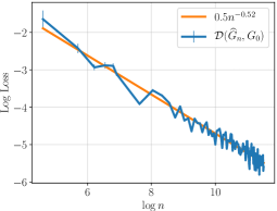
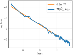
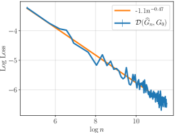
(a) Model A, $k=3$	(c) Model B, $k=4$	(e) Model C, $k=k_{0}=3$
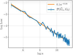
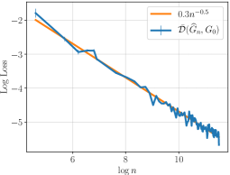
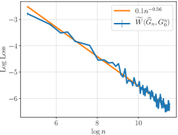
(b) Model A, $k=4$	(d) Model B, $k=5$	(f) Model C, $k=k_{0}=4$

Figure 2: Log-log scale plots for the simulation results under Models A–C. For each model and sample size $n$, we compute the estimator $\widehat{G}_{n}$ on 20 independent samples of size $n$. Its average discrepancy from the true mixing measure is plotted in blue, with error bars representing two empirical standard deviations. We additionally plot, in orange, the fitted linear regression line of these points, obtained using the method of least squares.

For each model, we generate 20 samples of size $n$, for 100 different choices of $n$ between $10^{2}$ and $10^{5}$. For each sample, we compute the penalized MLE $\widehat{G}_{n}$ with respect to the tuning parameter $\xi_{n}=\log n$, and with respect to a number of components $k$. For the fixed Models A–B, we choose $k\in\{k_{0}+1,k_{0}+2\}$, whereas for the varying Model C, we choose $k=k_{0}\in\{k^{*}+1,k^{*}+2\}$.

We report in Figure 2 the average discrepancy between $\widehat{G}_{n}$ and $G_{0}$ for each model and choice of $k$. The discrepancies are respectively taken to be $\mathcal{D},\macc@depth\char 1\relax\frozen@everymath{\macc@group}\macc@set@skewchar\macc@nested@a 111{}$ and $\widetilde{W}$ for Models A–C. In each case, it can be seen that the average discrepancy from $\widehat{G}_{n}$ to $G_{0}$ decays approximately at the rate $n^{-1/2}$, as was anticipated by Theorems 4,  5 and 6.

While these empirical convergence rates are similar across the three models, they imply vastly different convergence behaviors for the individual fitted parameters. For example, Figure 2(a) implies that $\widehat{G}_{n}$ has exactly two location parameters $\widehat{\mu}_{j}^{n}$ which converge to one of their population counterparts at the approximate rate $\alpha_{n}=n^{-1/4}$, and a third location parameter converging at the faster rate $\beta_{n}=n^{-1/2}$. Under Figure 2(e), a similar conclusion holds true, but now two possibilities arise: either $\alpha_{n}=n^{-1/6}$ and $\beta_{n}=n^{-1/2}$, or $\alpha_{n}=\beta_{n}=n^{-1/4}$. In contrast, past literature on mixture models only implies that the worst of these rates (i.e. $n^{-1/4}$ for Model A and $n^{-1/6}$ for Model C) hold for all three fitted parameters. The main contribution of our work was to show that such results are overly pessimistic, and that the fitted parameters of finite mixture models typically enjoy heterogeneous rates of convergence. In particular, a subset of the estimated parameters in finite mixture models may converge as fast as the parametric rate.

C.1 Numerical Specifications

We implement the penalized MLE $\widehat{G}_{n}$ using Algorithm 1, which is a slight modification of the EM algorithm Dempster et al., (1977) accounting for the penalty on the mixing proportions. This algorithm was previously discussed, for instance, by Chen and Khalili, (2008); Manole and Khalili, (2021), and only differs from the traditional EM algorithm for Gaussian mixture models through the update on line 6. We used Algorithm 1 as written for Model B, whereas for Models A and C, we omitted the update on line 8 for the scale parameters, and simply held them fixed to their true values.

Input: Starting values $\Psi^{(0)}=(\theta_{1}^{(0)},\dots,\theta_{k}^{(0)},\Sigma_{1}^{(0)},\dots,\Sigma_{k}^{(0)},\pi_{1}^{(0)},\dots,\pi_{k}^{(0)})$; i.i.d. sample $X_{1},\dots,X_{n}$; tuning parameter $\xi_{n}=\log n$; maximum number of iterations $T>0$; convergence criterion $\epsilon>0$.

1

2repeat

3      E-Step  :

4          Compute $w_{ij}^{(t+1)}\leftarrow\frac{\pi_{j}^{(t)}\log f(X_{i};\theta_{j}^{(t)},\Sigma_{j}^{(t)})}{\sum_{l=1}^{k}\pi_{l}^{(t)}\log f(X_{i};\theta_{l}^{(t)},\Sigma_{l}^{(t)})},\leavevmode\nobreak\ \leavevmode\nobreak\ i=1,\dots,n;\ j=1,\dots,k.$

5          

6           M-Step  :

7                For $j=1,\dots,k$,

8               $\pi_{j}^{(t+1)}\leftarrow\frac{\sum_{i=1}^{n}w_{ij}^{(t)}+\xi_{n}}{n+k\xi_{n}},$

9               $\mu_{j}^{(t+1)}\leftarrow\sum_{i=1}^{n}w_{ij}^{(t)}X_{i}/\sum_{i=1}^{n}w_{ij}^{(t)},$

10               $\Sigma_{j}^{(t+1)}\leftarrow\sum_{i=1}^{n}w_{ij}^{(t)}(X_{i}-\mu_{j}^{(t)})(X_{i}-\mu_{j}^{(t)})^{\top}/\sum_{i=1}^{n}w_{ij}^{(t)},$

11               $\Psi^{(t+1)}\leftarrow(\theta_{1}^{(t)},\dots,\theta_{k}^{(t)},\Sigma_{1}^{(t)},\dots\Sigma_{k}^{(t)},\pi_{1}^{(t)},\dots,\pi_{k}^{(t)}),$

12               $t\leftarrow t+1.$

13               

14               

15                until $\left\|\Psi^{(t)}-\Psi^{(t-1)}\right\|\leq\epsilon\leavevmode\nobreak\ \mathrm{or}\leavevmode\nobreak\ t\geq T$.

               Output: $\Psi^{(t)}$.

Algorithm 1 Modified EM Algorithm.

We chose the convergence criteria $\epsilon=10^{-8}$ and $T=2,000$. Since our aim is to illustrate theoretical properties of the estimator $\widehat{G}_{n}$, we initialized the EM algorithm favourably. In particular, for any given $k$ and $k_{0}$, and for each replication, we randomly partitioned the set $\{1,\dots,k\}$ into $k_{0}$ index sets $I_{1},\dots,I_{k_{0}}$, each containing at least one point. We then sampled $\theta_{j}^{(0)}$ (resp. $\Sigma_{j}^{(0)}$) from a Gaussian distribution with vanishing covariance, centered at $\theta_{\ell}^{0}$ (resp. $\Sigma_{\ell}^{0}$), where $\ell$ is the unique index such that $j\in I_{\ell}$.

References

- Ashtiani et al., (2020) Ashtiani, H., Ben-David, S., Harvey, N. J., Liaw, C., Mehrabian, A., and Plan, Y. (2020). Near-optimal sample complexity bounds for robust learning of Gaussian mixtures via compression schemes. Journal of the ACM, 67(6):1–42.
- Balakrishnan et al., (2017) Balakrishnan, S., Wainwright, M. J., and Yu, B. (2017). Statistical guarantees for the EM algorithm: From population to sample-based analysis. The Annals of Statistics, 45:77–120.
- Bechtel et al., (1993) Bechtel, Y. C., Bonaiti-Pellie, C., Poisson, N., Magnette, J., and Bechtel, P. R. (1993). A population and family study N-acetyltransferase using caffeine urinary metabolites. Clinical Pharmacology & Therapeutics, 54:134–141.
- Chen and Chen, (2003) Chen, H. and Chen, J. (2003). Tests for homogeneity in normal mixtures in the presence of a structural parameter. Statistica Sinica, pages 351–365.
- Chen, (1995) Chen, J. (1995). Optimal rate of convergence for finite mixture models. The Annals of Statistics, 23(1):221–233.
- Chen and Kalbfleisch, (1996) Chen, J. and Kalbfleisch, J. D. (1996). Penalized minimum-distance estimates in finite mixture models. Canadian Journal of Statistics, 24:167–175.
- Chen and Khalili, (2008) Chen, J. and Khalili, A. (2008). Order selection in finite mixture models with a nonsmooth penalty. Journal of the American Statistical Association, 103:187–196.
- Dempster et al., (1977) Dempster, A. P., Laird, N. M., and Rubin, D. B. (1977). Maximum likelihood from incomplete data via the EM algorithm. Journal of the Royal Statistical Society, Series B (Methodological), 39(1):1–38.
- Doss et al., (2020) Doss, N., Wu, Y., Yang, P., and Zhou, H. H. (2020). Optimal estimation of high-dimensional Gaussian mixtures. arXiv preprint arXiv:2002.05818.
- (10) Dwivedi, R., Ho, N., Khamaru, K., Wainwright, M. J., Jordan, M. I., and Yu, B. (2020a). Sharp analysis of Expectation-Maximization for weakly identifiable models. In Proceedings of the Twenty Third International Conference on Artificial Intelligence and Statistics, pages 1866–1876. PMLR.
- (11) Dwivedi, R., Ho, N., Khamaru, K., Wainwright, M. J., Jordan, M. I., and Yu, B. (2020b). Singularity, misspecification and the convergence rate of EM. The Annals of Statistics, 48:3161–3182.
- Folland, (1995) Folland, G. B. (1995). Introduction to Partial Differential Equations. Princeton University Press.
- Genovese and Wasserman, (2000) Genovese, C. R. and Wasserman, L. (2000). Rates of convergence for the Gaussian mixture sieve. The Annals of Statistics, 28:1105–1127.
- Ghosal and van der Vaart, (2001) Ghosal, S. and van der Vaart, A. W. (2001). Entropies and rates of convergence for maximum likelihood and Bayes estimation for mixtures of normal densities. The Annals of Statistics, 29:1233–1263.
- Guha et al., (2021) Guha, A., Ho, N., and Nguyen, X. (2021). On posterior contraction of parameters and interpretability in Bayesian mixture modeling. Bernoulli, 27(4):2159–2188.
- Hardt and Price, (2015) Hardt, M. and Price, E. (2015). Tight bounds for learning a mixture of two Gaussians. In Proceedings of the Forty-Seventh Annual ACM Symposium on Theory of Computing, pages 753–760.
- Heinrich and Kahn, (2018) Heinrich, P. and Kahn, J. (2018). Strong identifiability and optimal minimax rates for finite mixture estimation. The Annals of Statistics, 46(6):2844–2870.
- (18) Ho, N. and Nguyen, X. (2016a). Convergence rates of parameter estimation for some weakly identifiable finite mixtures. The Annals of Statistics, 44(6):2726–2755.
- (19) Ho, N. and Nguyen, X. (2016b). On strong identifiability and convergence rates of parameter estimation in finite mixtures. Electronic Journal of Statistics, 10:271–307.
- Ho and Nguyen, (2019) Ho, N. and Nguyen, X. (2019). Singularity structures and impacts on parameter estimation behavior in finite mixtures of distributions. SIAM Journal on Mathematics of Data Science, 1:730–758.
- Holzmann et al., (2004) Holzmann, H., Munk, A., and Stratmann, B. (2004). Identifiability of finite mixtures—with applications to circular distributions. Sankhyā: The Indian Journal of Statistics, pages 440–449.
- Kuusela et al., (2012) Kuusela, M., Vatanen, T., Malmi, E., Raiko, T., Aaltonen, T., and Nagai, Y. (2012). Semi-supervised anomaly detection—towards model-independent searches of new physics. In Journal of Physics: Conference Series, volume 368.
- Kwon et al., (2019) Kwon, J., Qian, W., Caramanis, C., Chen, Y., and Davis, D. (2019). Global convergence of the EM algorithm for mixtures of two component linear regression. In Conference on Learning Theory, pages 2055–2110.
- Manole and Ho, (2020) Manole, T. and Ho, N. (2020). Uniform convergence rates for maximum likelihood estimation under two-component Gaussian mixture models. arXiv preprint arXiv:2006.00704.
- Manole and Khalili, (2021) Manole, T. and Khalili, A. (2021). Estimating the number of components in finite mixture models via the Group-Sort-Fuse procedure. The Annals of Statistics, 49:3043–3069.
- McLachlan and Peel, (2004) McLachlan, G. and Peel, D. (2004). Finite mixture models. John Wiley & Sons.
- Nguyen, (2013) Nguyen, X. (2013). Convergence of latent mixing measures in finite and infinite mixture models. The Annals of Statistics, 4(1):370–400.
- Ohn and Lin, (2020) Ohn, I. and Lin, L. (2020). Optimal Bayesian estimation of Gaussian mixtures with growing number of components. arXiv preprint arXiv:2007.09284.
- Pele and Werman, (2009) Pele, O. and Werman, M. (2009). Fast and robust earth mover’s distances. In 2009 IEEE 12th International Conference on Computer Vision, pages 460–467. IEEE.
- van de Geer, (2000) van de Geer, S. (2000). Empirical Processes in M-estimation. Cambridge University Press.
- Wu and Yang, (2020) Wu, Y. and Yang, P. (2020). Optimal estimation of Gaussian mixtures via denoised method of moments. The Annals of Statistics, 48:1987–2007.