The role of slow magnetostrophic waves in the formation of the axial dipole in planetary dynamos

Abstract

The preference for the axial dipole in planetary dynamos is investigated through the analysis of wave motions in spherical dynamo models. Our study focuses on the role of slow magnetostrophic waves, which are generated from localized balances between the Lorentz, Coriolis and buoyancy (MAC) forces. Since the slow waves are known to intensify with increasing field strength, simulations in which the field grows from a small seed towards saturation are useful in understanding the role of these waves in dynamo action. Axial group velocity measurements in the energy-containing scales show that fast inertial waves slightly modified by the magnetic field and buoyancy are dominant under weak fields. However, the dominance of the slow waves is evident for strong fields satisfying $|\omega_{M}/\omega_{C}|\sim$ 0.1, where $\omega_{M}$ and $\omega_{C}$ are the frequencies of the Alfvén and inertial waves respectively. A MAC wave window of azimuthal wavenumbers is identified wherein helicity generation by the slow waves strongly correlates with dipole generation. Analysis of the magnetic induction equation suggests a poloidal–poloidal field conversion in the formation of the dipole. Finally, the attenuation of slow waves may result in polarity reversals in a strongly driven Earth’s core.

1 Introduction

Planetary dynamos are driven by thermochemical convection in their fluid cores. The axial dipole dominates a large region of the parameter space in convection-driven dynamos where the effect of planetary rotation, measured by the Coriolis forces, is large relative to that of both nonlinear inertia and viscosity (Sreenivasan and Jones, 2006, 2011; Schaeffer et al., 2017). Rapid rotation produces anisotropic convection with equatorially antisymmetric axial motions, the helicity of which is thought to be essential for dynamo action (Moffatt, 1978; Olson et al., 1999). A long-standing question in planetary dynamo theory is whether the preference for the axial dipole is due to a purely kinematic process influenced by rotation or due to a magnetohydrodynamic process influenced by both rotation and the self-generated magnetic field. Answering this question would also help us constrain the parameter space that admits polarity reversals in strongly driven dynamos (e.g. Sreenivasan et al., 2014).

An early study by Busse (1976) used the linear theory of magnetoconvection to explore the onset of dynamo action in an annulus. Busse found that the effect of a magnetic field on convection enhanced magnetic field generation. This interesting idea was explored further by Sreenivasan and Jones (2011) who showed that the presence of a magnetic field substantially enhanced the kinetic helicity of columnar convection. They considered linear magnetoconvection in a spherical shell in the rapidly rotating limit $E\to 0$, where $E$ is the Ekman number that gives the ratio of viscous to Coriolis forces. Although the spatially varying magnetic field in a nonlinear dynamo does not substantially lower the threshold for convective onset relative to that in the nonmagnetic system (Sreenivasan and Gopinath, 2017), there is a substantial enhancement of helical convection in the neighbourhood of the length scale of energy injection (Sreenivasan and Kar, 2018). The growth of convection is notably absent in a kinematic dynamo, which fails to produce the axial dipole with the same parameters and initial conditions. While nonlinear dynamo models strongly relate field-induced helicity generation in the energy-containing scales to dipole formation, the primary force balance in these scales is known to be approximately geostrophic (Aurnou and King, 2017; Aubert et al., 2017), which raises the question of how the field acts on these scales so as to enhance helicity. The present study addresses this question by analyzing wave motions in the energy-containing scales in planetary dynamo models.

Wave motions in planetary cores arise from the effects of rotation, magnetic field and buoyancy. Torsional oscillations propagating radially at the Alfvén speed across concentric cylinders have been simulated in low-inertia numerical models of the geodynamo (Wicht and Christensen, 2010; Teed et al., 2014). Non-axisymmetric Alfvén waves propagating along the cylindrical radius are conceivable (Jault, 2008; Bardsley and Davidson, 2016; Aubert and Finlay, 2019) since the convection is made up of thin columns aligned with the rotation axis. Slow Magneto-Coriolis (MC) Rossby waves, thought to produce the westward drift of the Earth’s magnetic field, have been realized in dynamo simulations (Hori et al., 2015). While convection can onset in the form of Alfvén waves in a non-rotating Bénard layer (Roberts and Zhang, 2000), the planetary regime of strong rotation can support convection through fast and slow Magnetic-Archimedean-Coriolis (MAC) waves. The fast MAC waves are inertial waves weakly modified by the magnetic field and buoyancy; the slow MAC, or magnetostrophic, waves are slow MC waves modified by buoyancy (Braginsky, 1967; Busse et al., 2007). Buoyancy-driven fast inertial waves generate and segregate oppositely signed helicity in spherical dynamos (Ranjan et al., 2018). That said, the intensity of slow MAC wave motions would be comparable to that of the fast waves for $|\omega_{M}/\omega_{C}|\sim$ 0.1, where $\omega_{M}$ and $\omega_{C}$ are the Alfvén wave and inertial wave frequencies respectively (Sreenivasan and Maurya, 2021). Here, we examine the role of the slow MAC waves in helicity generation in the energy-containing scales of the dynamo, and hence in axial dipole formation. While earlier studies have related axisymmetric MAC waves in the stably stratified layer at the top of the core to the decadal oscillations in the Earth’s field (Buffett et al., 2016), the focus of the present study is to relate non-axisymmetric MAC waves in an unstably stratified core to the formation of the dipole field. Because slow MAC waves intensify with increasing field strength, a nonlinear simulation in which the field grows from a small seed towards saturation would help us understand when the slow waves have a dominant presence alongside the fast waves in the dynamo.

Numerical dynamo models (Olson et al., 1999; Kageyama and Sato, 1997) have shown how columnar vortices twist the toroidal magnetic field lines to produce the poloidal field. Takahashi and Shimizu (2012) and Peña et al. (2018) made a detailed analysis of terms in the magnetic induction equation. The present study looks at the dominant contributions to the axial dipole field and brings out the differences between kinematic and nonlinear dynamos in this respect.

In Section 2, we describe the dynamo model and define the main dimensionless parameters used in this study. Section 3 builds on a recent study that suggested field-induced helicity generation in the relatively large scales of the dynamo (Sreenivasan and Kar, 2018) and shows through force balances that local magnetostrophy can exist in these scales where the Lorentz forces are small in the global balance. Section 4 analyses the fundamental frequencies in the dynamo and shows that the MAC wave window of azimuthal wavenumbers is indeed where the axial dipole is predominantly generated. In Section 5, the slow MAC waves in nonlinear dynamo simulations are identified by group velocity measurements. Section 6 gives the contributions to the axial dipole of the dominant terms in the induction equation in nonlinear and kinematic dynamo simulations. In conclusion, the main results of this study are summarized and its implications for polarity reversals in strongly driven dynamos are discussed.

2 Numerical dynamo model

We consider dynamo action in an electrically conducting fluid confined between two concentric, corotating spherical surfaces that correspond to the inner core boundary (ICB) and the CMB. The ratio of inner to outer radius is 0.35. Fluid motion is driven by thermal buoyancy-driven convection, although our set of equations may also be used to study thermochemical convection using the codensity formulation (Braginsky and Roberts, 1995). The other body forces acting on the fluid are the Lorentz force, arising from the interaction between the induced electric currents and the magnetic fields and the Coriolis force originating from the background rotation. The governing equations are those in the Boussinesq approximation (Kono and Roberts, 2002). Lengths are scaled by the thickness of the spherical shell $L$, and time is scaled by the magnetic diffusion time, $L^{2}/\eta$, where $\eta$ is the magnetic diffusivity. The velocity field ${\bm{u}}$ is scaled by $\eta/L$, the magnetic field ${\bm{B}}$ is scaled by $(2\varOmega\rho\mu\eta)^{1/2}$ where $\varOmega$ is the rotation rate, $\rho$ is the fluid density and $\mu$ is the magnetic permeability. The root mean square (rms) and peak values of the scaled magnetic field (Elsasser number $\varLambda$) are outputs derived from our dynamo simulations, where the mean is a volume average.

The non-dimensional MHD equations for the velocity, magnetic field and temperature are given by,

$$EPm^{-1}\Bigl{(}\frac{\partial{\bm{u}}}{\partial t}+(\nabla\times{\bm{u}})\times{\bm{u}}\Bigr{)}+{\hat{\bm{z}}}\times{\bm{u}}=-\nabla p^{\star}+Ra\,E\,PmPr^{-1}\,T\,{\bm{r}}\,$$

$$+(\nabla\times{\bm{B}})\times{\bm{B}}+E\nabla^{2}{\bm{u}},$$ (1)

$$\frac{\partial{\bm{B}}}{\partial t}=\nabla\times({\bm{u}}\times{\bm{B}})+\nabla^{2}{\bm{B}},$$ (2)

$$\frac{\partial T}{\partial t}+({\bm{u}}\cdot\nabla)T=PmPr^{-1}\,\nabla^{2}T,$$ (3)

$$\nabla\cdot{\bm{u}}=\nabla\cdot{\bm{B}}=0,$$ (4)

The modified pressure $p^{*}$ in equation (1) is given by $p+E\,Pm^{-1}\,|\bm{u}|^{2}$. The dimensionless parameters in the above equations are the Ekman number $E=\nu/2\varOmega L^{2}$, the Prandtl number, $Pr=\nu/\kappa$, the magnetic Prandtl number, $Pm=\nu/\eta$ and the Rayleigh number $g\alpha L\Delta T/2\Omega\kappa$. Here, $g$ is the gravitational acceleration, $\nu$ is the kinematic viscosity, $\kappa$ is the thermal diffusivity and $\alpha$ is the thermal expansion coefficient.

The basic-state temperature profile represents a basal heating given by $T_{0}(r)=\beta/r$, where $\beta$ is a constant. We set isothermal conditions at both boundaries. The velocity and magnetic fields satisfy the no-slip and electrically insulating conditions, respectively (Sreenivasan and Jones, 2006). The calculations are performed by a pseudospectral code that uses spherical harmonic expansions in the angular coordinates $(\theta,\phi)$ and finite differences in radius $r$ (Willis et al., 2007).

3 Helicity generation during magnetic field growth from a seed

Table 1: Summary of the key important input and output parameters in the dynamo simulations considered in the present study. Here, $N_{r}$ is the number of radial grid points, $l_{max}$ is the maximum spherical harmonic degree, $\bar{B}$ is the volume-averaged root mean square value of the magnetic field, $B^{P}_{10}$ is the poloidal axial dipole field, $Ra_{c}$ is the critical Rayleigh number for the onset of nonmagnetic convection, $Rm$ is the magnetic Reynolds number, and $l_{c}$ and $l_{E}$ are the mean spherical harmonic degrees for convection and energy injection respectively, defined in (5). The values in brackets are those for the reference nonmagnetic runs.

S.No.	$E$	$Ra$	$Ra/Ra_{c}$	$Pm$	$Pr$	$N_{r}$	$l_{max}$	$\bar{B}$	$B^{P}_{10}$	$Rm$	$l_{c}$	$l_{E}$
a	$1.2\times 10^{-5}$	220	4.2	5	5	120	100	0.7	0.30	105	21 (28)	20 (29)
b	$1.2\times 10^{-5}$	500	9.6	5	5	144	120	1.68	0.80	184	23 (34)	23 (32)
c	$1.2\times 10^{-5}$	1000	19.2	5	5	168	176	2.31	0.88	326	26 (35)	29 (37)
d	$1.2\times 10^{-5}$	2000	38.5	5	5	192	224	3.05	0.96	558	28 (39)	33 (40)
e	$1.2\times 10^{-5}$	5000	96.1	5	5	180	224	3.79	0.87	1218	31 (22)	42 (31)
f	$1.2\times 10^{-5}$	15000	288.4	5	5	288	280	6.21	0.84	2710	33 (21)	46 (36)
g	$1.2\times 10^{-6}$	400	7.3	1	1	192	220	0.86	0.3	215	39 (43)	31 (49)

In line with an earlier studies (Sreenivasan and Jones, 2011; Sreenivasan and Kar, 2018), we examine the evolution of the dynamo from an initial dipole-dominated seed magnetic field of intensity $\overline{B}=0.01$. The initial velocity field is the same as that in the equivalent saturated non-magnetic run. The key input and output parameters of the simulations, given in table 1, are time-averaged values in the saturated state of the dynamo. Here, the mean spherical harmonic degrees for convection and energy injection are defined by

$$l_{c}=\dfrac{\Sigma\hskip 1.0ptl\hskip 1.0ptE_{k}(l)}{\Sigma\hskip 1.0ptE_{k}(l)};\hskip 5.0ptl_{E}=\dfrac{\Sigma\hskip 1.0ptl\hskip 1.0ptE_{T}(l)}{\Sigma\hskip 1.0ptE_{T}(l)},$$ (5)

where $E_{k}(l)$ is the kinetic energy spectrum and $E_{T}(l)$ is the spectrum obtained from the product of $u_{r}T$ and its conjugate.

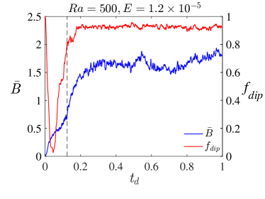
(a)

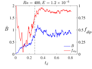
(b)

Figure 1: Evolution in time (measured in units of magnetic diffusion time) of the magnetic field intensity given by its volume averaged root mean square value, $\bar{B}$ and $f_{dip}$ (a measure of the axial dipole strength). The dipole formation time, marked by the vertical dashed line, is at $t_{d}=0.125$ in (a) and $t_{d}=0.28$ in (b).

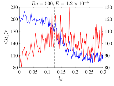
(a)

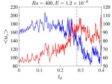
(b)

Figure 2: Root mean square value of the axial velocity $u_{z}$ for two ranges of spherical harmonic degree, l. The scales considered are $l\leq 23$ (red) in (a) and $l\leq 31$ (red) in (b), $l>23$ (blue) in (a) and $l>31$ (blue) in (b). The mean harmonic degree of energy injection $l_{E}$ serves as the basis for separation of scales.

The value of $f_{dip}$, which measures the relative energy contained in the axial dipole (Christensen and Aubert, 2006), shows that the field loses its dipolar character and only regains it after passing through a non-dipolar phase (figure 1). The snapshots of the radial field at the core–mantle boundary during this process can be found in a previous paper (Sreenivasan and Kar, 2018) and hence not reproduced here. Dynamo saturation occurs only later than dipole formation. The time for formation of dipole decreases at high $Ra$. The progressive increase of the magnetic field intensity during dynamo evolution is accompanied by an increase of the convective velocity in the “large” energy-containing scales. The scales are separated by the mean harmonic degree of energy injection, $l_{E}$. There is little or no increase of the velocity in the scales $l>l_{E}$. From figure 2, we note that the time of formation of the dipole roughly corresponds with the saturation of the axial velocity $u_{z}$ in the large scales. For the moderate forcing considered here ($Ra/Ra_{c}\sim 10$), the extraction of kinetic energy from the small scales, due to the Lorentz force occurs only near the formation of the dipole. The magnetic field is fed by this kinetic energy but the growth of magnetic energy is not much due to this process. The extraction of energy occurs in a relatively short time. Thus, the growth of energy in the large scales and extraction of energy from the small scales remains fairly independent. We might hypothesize that a quasi-linear wave excitation in the large scales of the dynamo would cause the enhancement of convective velocity over that in the equivalent nonmagnetic state. As the forcing is increased, the extraction of energy from the small scales happens before the formation of the dipole. This would mean that at higher $Ra/Ra_{c}$, the growth of magnetic field is partially fed by the kinetic energy from the small scales.

Figure 3 (a) and (b) show the enhancement of kinetic helicity in the large scales for the two dynamo simulations considered in figure 2. In cylindrical coordinates $(s,\phi,z)$, the magnetic field enhances the axial ($z$) and radial ($s$) parts of the helicity in equal measure (Sreenivasan and Jones, 2011). Therefore, the sum of the $z$ and $s$ parts of the helicity is considered. A notable finding is that the dipole forms from a chaotic multipolar state when the helicity in the large scales increases by a magnitude nearly equal to the initial helicity in these scales, associated with convection in the equivalent nonmagnetic system. Table 2 shows the sum of peak $z$ and $s$ helicity attained during the growth of the magnetic field for the lower half of the shell. For moderate $Ra$, the total helicity over all scales during the growth of the magnetic field is higher than the nonmagnetic value as extraction of kinetic energy from the small scales occurs only near the dipole formation time. This is illustrated in figure 3 (c), where at $t_{d}=0.26$, peak helicity growth occurs such that the helicity in the dynamo exceeds the nonmagnetic helicity for all scales. By time $t_{d}=0.28$ (figure 3 (d)), energy extraction would begin and the helicity in the small scales would fall below the nonmagnetic values. By the time the dynamo reaches saturation, the helicity in the small scales would have fallen even further. The helicity deficit in the small scales dominates the helicity generated in the large scales and therefore the total helicity in the saturated dynamo is always less than its nonmagnetic counterpart. For higher $Ra$, the total helicity would always be the less than that in the nonmagnetic case as the energy extraction from the small scales occurs much before dipole formation. The helicity in the large scales would, however, still exceed the helicity of the nonmagnetic case.

Ranjan et al. (2020) show that the helicity source term due to the Lorentz force is negatively correlated with the overall helicity distribution. They attributed the distribution of helicity in the core to inertial waves. No scale separation was performed, so the overall helicity for the saturated dynamo was lower than that for the nonmagnetic state. Their result is consistent with our analysis considering all scales (table 2). To show that the slow MAC waves might cause the increase of dynamo helicity over the nonmagnetic value at scales $l\leq l_{E}$, one must first look at the scale-separated force balance in the dynamo.

Table 2: Sum of the axial ($z$) and and radial ($s$) parts of the kinetic helicity for the large (energy-containing) scales and for all scales evaluated at two times during the evolution of the dynamo magnetic field from a seed state. The helicity is evaluated for the lower half of the spherical shell. The nonmagnetic helicity is given in brackets. The large scales are those for $l\leq l_{E}$, where $l_{E}$ is the mean harmonic degree of energy injection in the dynamo.

S.No.	$E$, $Ra$	time ($t_{d}$)	Scales	Helicity
(i)	$1.2\times 10^{-5}$ , 500	0.095	$l\leq 23$	$3.21\times 10^{5}$ $(1.34\times 10^{5})$
			All	$7.66\times 10^{6}$  $(7.23\times 10^{6})$
		0.125	$l\leq 23$	$2.81\times 10^{5}$ $(1.34\times 10^{5})$
			All	$6.41\times 10^{6}$  $(7.23\times 10^{6})$
(ii)	$1.2\times 10^{-6}$, 400	0.26	$l\leq 31$	$6.89\times 10^{5}$ $(3.05\times 10^{5})$
			All	$7.15\times 10^{6}$  $(4.85\times 10^{6})$
		0.28	$l\leq 31$	$6.72\times 10^{5}$ $(3.05\times 10^{5})$
			All	$3.89\times 10^{6}$  $(4.85\times 10^{6})$

3.1 Scale-dependent balance of forces

Dipole-dominated dynamos are known to exist in the so-called MAC regime where Lorentz, buoyancy and Coriolis forces are dominant (Sreenivasan and Jones, 2006, 2011) and the nonlinear inertial and viscous forces are negligible. The Lorentz forces may, however, be localized due to spatially inhomogeneous magnetic flux. In line with earlier studies (Sreenivasan and Jones, 2006), we examine the ratio of the Lorentz, Coriolis and buoyancy forces in the $z$ vorticity equation to the highest force among them for two distinct ranges of the spherical harmonic degree.

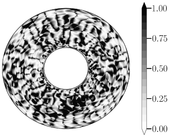
(a)               M

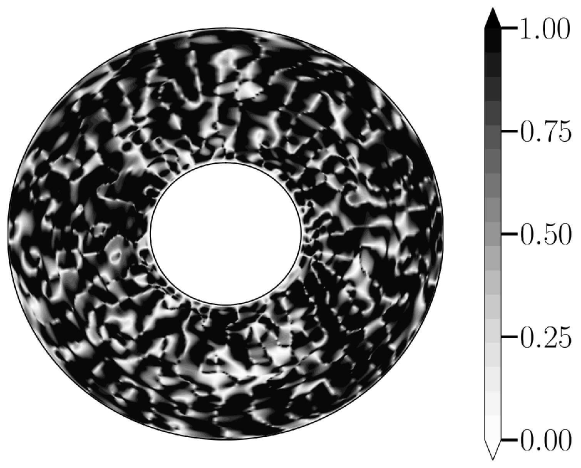
(b)               A

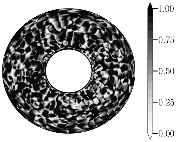
(c)                C

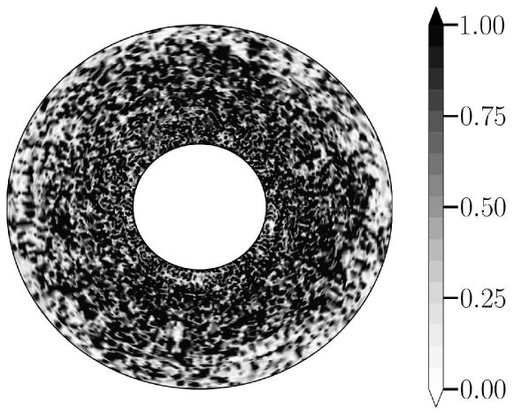
(d)               M

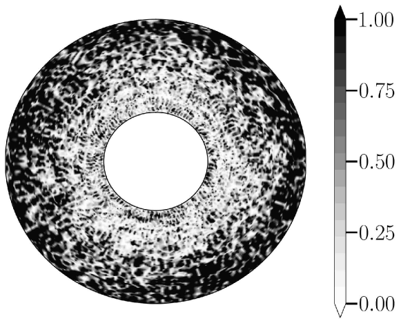
(e)               A

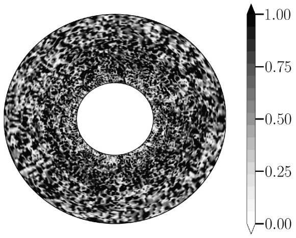
(f)               C

Figure 4: The ratio of magnitudes of the magnetic Lorentz (M), buoyancy (A) and Coriolis (C) force terms in the $z$-vorticity equation to the magnitude of the largest force among them, is plotted on the horizontal section $z=0.1$ for two ranges of scales $l\leq 31$ in ((a)-(c)) and $l>100$ in ((d)-(f)). The model parameters are $Ra=400$, $Pm=Pr=1$, $E=1.2\times 10^{-6}$.

In the dynamo simulation at $E=1.2\times 10^{-6}$ and $Ra=400$, the Coriolis and buoyancy forces are in approximate balance for the relatively large scales $l\leq 31$ (figure 4 (b) and (c)). However, as seen in figure 4(a), the Lorentz forces become significant in patches and balance the Coriolis forces. Therefore, local excitation of slow MAC waves in these scales is conceivable. For the small scales of $l>100$, the buoyancy forces are restricted to the outer periphery of the shell (figure 4 (e)). The dominant balance in these scales is between the Lorentz and Coriolis forces (figure 4 (d) and 4 (f)). In either range of harmonic degrees, the nonlinear inertial and viscous forces are small compared with the other forces in the bulk of the volume, and hence not shown.

Before discussing the role of the slow MAC waves in the dynamo, we examine the relative magnitudes of the fundamental frequencies and show that wave motions correlate with helicity generation and dipole formation in the energy-containing scales.

4 MAC waves, helicity and dipole formation

In the absence of magnetic diffusion, the roots of the following characteristic equation (Busse et al., 2007; Sreenivasan and Maurya, 2021) give the frequencies of waves produced in a rotating stratified fluid layer subject to a magnetic field:

$$(\omega^{2}-\omega_{M}^{2}-\omega_{A}^{2})(\omega^{2}-\omega_{M}^{2})-\omega_{C}^{2}\omega^{2}=0,$$ (6)

where the fundamental frequencies $\omega_{M}$, $\omega_{A}$ and $\omega_{C}$ represent Alfvén waves, internal gravity waves and linear inertial waves respectively. In unstable stratification that drives planetary core convection, $\omega_{A}^{2}<0$, where $|\omega_{A}|$ is simply a measure of the strength of buoyancy. The dimensionless values of $\omega_{M}^{2}$, $-\omega_{A}^{2}$ and $\omega_{C}^{2}$ in the dynamo are given by

$$\omega_{M}^{2}=\frac{Pm}{E}(\bm{B}\cdot{\bm{k}})^{2},\quad-\omega_{A}^{2}=\frac{Pm^{2}Ra}{Pr\,E}\,\left(\frac{{k_{z}}^{2}+m^{2}}{k^{2}}\right),\quad\omega_{C}^{2}=\frac{Pm^{2}}{E^{2}}\frac{k_{z}^{2}}{k^{2}},$$ (7)

where $k_{s}$, $m$ and $k_{z}$ are the radial, azimuthal and axial wavenumbers in cylindrical coordinates $(s,\phi,z)$, and $k$ is the resultant wavenumber. Here, $\omega_{A}$ is evaluated on the equatorial plane where the buoyancy force is maximum; $\omega_{M}$ is based on the measured peak magnetic field in the dynamo. Using the scaling for time in the dynamo model, the frequencies in (7) are scaled by $\eta/L^{2}$.

For the inequality $\omega_{C}>\omega_{M}>\omega_{A}$, the roots of equation (6),

$$\omega_{f}=\pm\frac{1}{\sqrt{2}}\sqrt{\omega_{A}^{2}+\omega_{C}^{2}+2\omega_{M}^{2}+\sqrt{\omega_{A}^{4}+2\omega_{A}^{2}\omega_{C}^{2}+4\omega_{M}^{2}\omega_{C}^{2}+\omega_{C}^{4}}},$$ (8)

$$\omega_{s}=\pm\frac{1}{\sqrt{2}}\sqrt{\omega_{A}^{2}+\omega_{C}^{2}+2\omega_{M}^{2}-\sqrt{\omega_{A}^{4}+2\omega_{A}^{2}\omega_{C}^{2}+4\omega_{M}^{2}\omega_{C}^{2}+\omega_{C}^{4}}}.$$ (9)

represent the fast ($f$) and slow ($s$) MAC waves. While the fast waves are linear inertial waves weakly modified by the magnetic field and buoyancy, the slow waves are magnetostrophic (Braginsky, 1967; Acheson and Hide, 1973; Busse et al., 2007; Sreenivasan and Maurya, 2021).

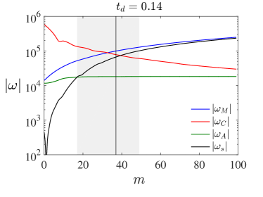
(a)

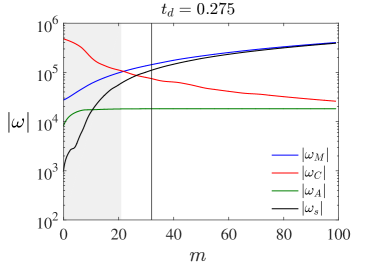
(b)

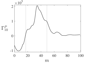
(c)

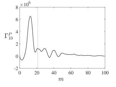
(d)

Figure 5: (a) & (b): Absolute values of frequencies plotted for two snapshots of time during the evolution of the dynamo from a small seed field magnetic field. The magnitudes of the following frequencies are shown: $\omega_{C}$ (linear inertial wave), $\omega_{M}$ (Alfvén wave), $\omega_{A}$ (internal gravity wave) and $\omega_{s}$ (slow MAC wave). Since $\omega_{A}^{2}<0$ in unstable stratification, $\omega_{A}$ is simply a measure of the strength of buoyancy in the dynamo. The shaded grey area shows the scales where helicity is generated in the dynamo simulation relative to the nonmagnetic simulation. The thin solid vertical line shows the mean wave number of energy injection. (c) & (d): Contribution to the axial dipole energy per unit time, $\int_{V}\bm{B}^{P}_{10}.[\bm{\nabla}\times(\bm{u}\times\bm{B})]dV$ plotted as a function of the spherical harmonic order, $m$. The vertical dotted lines show the same range of scales as in (a) & (b), where helicity is generated. The dynamo parameters are $Ra=400$, $Pm=Pr=1$, $E=1.2\times 10^{-6}$.

In figure 5(a) and (b), the magnitudes of the fundamental frequencies are shown as a function of the azimuthal wavenumber $m$. Two times are analysed in the growth phase of the dynamo run at $E=1.2\times 10^{-6}$, $Ra=400$ and $Pr=Pm=1$. The frequencies are computed from (7) using the mean values of the $s$ and $z$ wavenumbers. For example, real space integration over $(s,\phi)$ gives the kinetic energy as a function of $z$, the Fourier transform of which gives the one-dimensional spectrum $\hat{u}^{2}(k_{z})$. Subsequently, we obtain

$$\bar{k}_{z}=\frac{\Sigma k_{z}\,\hat{u}^{2}(k_{z})}{\Sigma\hat{u}^{2}(k_{z})}.$$ (10)

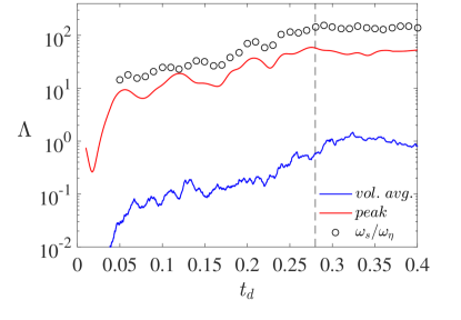
Figure 14: Peak and volume-averaged values of the Elsasser number $\varLambda$ shown against magnetic diffusion time, starting from the initial seed field state to the saturated state of the dynamo. The symbols (circles) represent the instantaneous values of $\omega_{s}/\omega_{\eta}$, where $\omega_{s}$ is the slow MAC wave frequency and $\omega_{\eta}$ is the magnetic diffusion frequency. The dashed vertical line marks the dipole formation time. The dynamo simulation has the parameters $Ra=400$, $Pm=Pr=1$, $E=1.2\times 10^{-6}$.

A similar approach gives $\bar{k}_{s}$. The computed frequencies in figure 5(a) and (b) satisfy the inequality $|\omega_{C}|>|\omega_{M}|>|\omega_{A}|$ in the energy-containing scales of the dynamo spectrum, indicating that the MAC waves would be generated in these scales. We emphasize that this inequality would be obtained only if the measured peak magnetic field is used in the evaluation of $\omega_{M}$, corresponding to local Elsasser numbers $\varLambda\gg 1$ (see Sreenivasan and Maurya (2021) and figure 14 in Section 7). The range of scales with the above frequency inequality narrows as the field intensity increases in time, and close to dipole formation ($t_{d}=0.275$), this inequality is confined to wavenumbers $m<19$. The scales of helicity generation, shown in shaded grey bands, are obtained from the differences between the helicity spectra of the magnetic and equivalent non-magnetic runs. Notably, the region of helicity generation overlaps with the scales where the MAC waves are generated. The slow MAC wave frequency merges with the Alfvén wave frequency at large $m$, where $\omega_{M}$ is the dominant frequency.

The contribution of convection to the axial dipole field energy per unit time is given by (e.g. Buffett and Bloxham, 2002)

$$\Gamma^{P}_{10}=\int_{V}\bm{B}^{P}_{10}\cdot[\mathbf{\nabla}\times(\bm{u}\times\bm{B})]dV.$$ (11)

The spectral distribution of $\Gamma^{P}_{10}$ is shown in figure 5 (c) and (d). Evidently, the maximum contribution to the dipole energy occurs in the scales where helicity is generated by the magnetic field. The strong correlation between MAC wave formation, helicity generation, and in turn, the axial dipole field energy, is also noted in the dynamo simulation at $E=10^{-5}$.

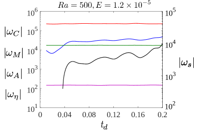
(a)

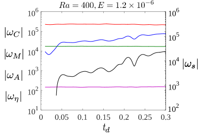
(b)

Figure 6: Absolute values of the dynamo frequencies plotted against time (in units of the magnetic diffusion time $t_{d}$). Both the simulations study the evolution of the dynamo starting from a small seed magnetic field. The frequencies are calculated at the mean azimuthal wavenumber ($\bar{m}=$10 for (a) and 11 for (b)) of the range of scales where MAC waves are active at dipole formation time. The axial dipole forms from a multipolar state at $t_{d}\approx 0.125$ in (a) and $t_{d}\approx 0.28$ in (b). The frequencies shown (with line colours in brackets) are as follows: $\omega_{M}$ (blue), $\omega_{C}$ (red), $\omega_{A}$ (green), $\omega_{\eta}$ (magenta), $\omega_{s}$ (black).

Figure 6(a) and (b) shows the fundamental frequencies and the slow MAC wave frequency plotted against time for two dynamo simulations that begin from a small seed magnetic field. The frequencies are calculated at mean azimuthal wavenumber of the range of scales where the slow waves are thought to be active at dipole formation time. The dimensionless magnetic diffusion frequency $\omega_{\eta}$ is given by $(\bar{k}L)^{2}$. It is evident that the frequency inequality $|\omega_{C}|>|\omega_{M}|>|\omega_{A}|>|\omega_{\eta}|$ is satisfied at times approaching axial dipole formation and beyond. The slow MAC waves, whose frequency $\omega_{s}$ is given by the black solid line, are generated for $|\omega_{M}|>|\omega_{A}|$, since (Braginsky, 1967; Busse et al., 2007)

$$\omega_{s}\approx\frac{\omega_{M}^{2}}{\omega_{C}}\left(1+\frac{\omega_{A}^{2}}{\omega_{M}^{2}}\right)^{1/2},$$ (12)

where $\omega_{M}^{2}/\omega_{C}$ is the Magneto-Coriolis (MC) wave frequency.

$E=1.2\times 10^{-5}$, $Ra=500$			$E=1.2\times 10^{-6}$, $Ra=400$
$t_{d}$	$\omega_{M}/\omega_{C}$	$Le$	$t_{d}$	$\omega_{M}/\omega_{C}$	$Le$
0.033	0.108	0.005	0.041	0.076	0.003
0.04	0.147	0.006	0.14	0.162	0.0065
0.125	0.310	0.014	0.28	0.345	0.014

Table 3: Comparison of the values of the Lehnert number $Le$ and the frequency ratio $\omega_{M}/\omega_{C}$ at three points in time (in units of the magnetic diffusion time $t_{d}$) during the growth phase of two dynamo models. The times considered are those at incipient slow MAC wave generation, onset of helicity generation, and axial dipole formation. The evolution in time of the measured frequencies in these models is shown in figure 6(a) and (b).

The Lehnert number in the dynamo simulations, evaluated by

$$Le=|\bm{B}|\left(\frac{E}{Pm}\right)^{1/2}\,\frac{m}{2\pi},$$

has its origin in $(\omega_{M}/\omega_{C})_{0}$, the frequency ratio at the initial state of a buoyant blob released into the flow (Sreenivasan and Maurya, 2021). As blobs evolve in time into columns, the wavenumbers $k_{s}$ and $k_{z}$ decrease relative to $m$, so the instantaneous value of $(\omega_{M}/\omega_{C})$ is at least one order of magnitude higher than $Le$ (table 3). For values of $(\omega_{M}/\omega_{C})\sim 0.1$, the intensity of slow MAC wave motions would be comparable to that of the fast waves (Sreenivasan and Maurya, 2021). Consequently, one would expect the helicity generated by the slow wave motions to be of the same order of magnitude as that of the fast waves. The approximately two-fold increase in the helicity as the dynamo evolves from a seed magnetic field (figure 3 (a) & (b)) suggests that the helicity generated by slow wave motions in the dynamo may be comparable to that produced by the fast inertial waves in nonmagnetic convection.

While the frequency diagrams in figure 5 and figure 6 suggest the active role of slow MAC waves in dipole formation, conclusive evidence for the existence of these waves necessitates visualization of their propagation, which is presented in the following section.

5 Identification of slow MAC waves in the dynamo

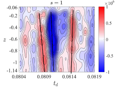
(a)

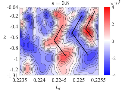
(b)

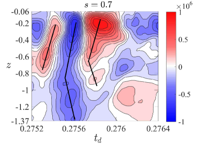
(c)

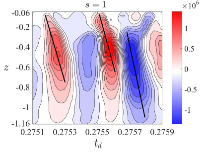
(d)

Figure 7: (a) Contour plot of $\dot{u_{z}}$ for the time interval $t_{d}=$0.08–0.083 and $l\leq 42$. (b) $\dot{u_{z}}$ for the time interval $t_{d}=$0.224–0.225 and $l\leq 36$. (c) & (d) $\dot{u_{z}}$ for the time interval $t_{d}=$0.274–0.278 and $l\leq 31$. The cylindrical radius $s$ at which each plot is produced is given above the respective panel. The parameters of the dynamo simulation are $E=1.2\times 10^{-6}$, $Ra=400$, $Pm=Pr=1$. The black lines indicate the direction of travel of the waves and their slope gives the group velocity. The estimated group velocity of the fast and slow MAC waves ($U_{f}$ and $U_{s}$ respectively) and the measured group velocity $U_{g,z}$ are given in table 4.

Wave motions in the dynamo are analysed through contour plots of $\dot{u_{z}}$ at points on different cylindrical radii $s$ and for small windows of time spanning the evolution of magnetic field in the simulation (e.g. figure 7). Analysis of a dynamo simulations in which the field increases from a small seed value gives a good insight into the conditions for the dominance of fast and slow MAC waves. Attention is focused on the energy containing scales $l\leq l_{E}$, in which the mean azimuthal wavenumber $\bar{m}$ is calculated over the range where the inequality $|\omega_{C}|>|\omega_{M}|>|\omega_{A}|$ supports the formation of the MAC waves. The axial group velocity measured from the contour plots ($U_{g,z}$) is compared with the estimated value ($U_{f}$, $U_{s}$) obtained by taking the derivative of the fast ($f$) and slow ($s$) wave frequencies with respect to $k_{z}$ (table 4).

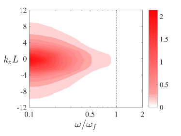
(a)

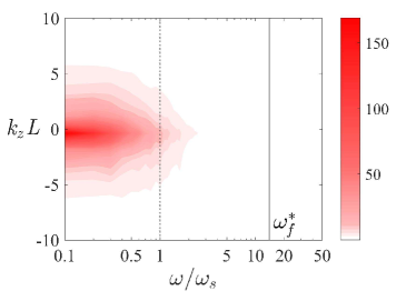
(b)

Figure 8: (a) $\phi$-averaged FFT of $\dot{u_{z}}$ at cylindrical radius $s=0.7$ for the scales $l\leq 42$ in the time interval $t_{d}=0.08-0.082$. (b) $\phi$-averaged FFT of $\dot{u_{z}}$ at $s=0.7$ for $l\leq 31$ in the time interval $t_{d}=0.274-0.278$. The range $l\leq l_{E}$ narrows down as the field intensity increases with time. The dynamo parameters are $Ra=400$, $Pm=Pr=1$, $E=1.2\times 10^{-6}$. The dotted vertical lines correspond to $\omega/\omega_{f}=1$ in (a) and $\omega/\omega_{s}=1$ in (b), where $\omega_{f}$ and $\omega_{s}$ are the estimated fast and slow MAC wave frequencies. In (b), $\omega^{*}_{f}$ = $\omega_{f}/\omega_{s}$.

Figure 7 shows the measurement of wave motion in the dynamo simulation with $E=1.2\times 10^{-6}$ and $Ra=400$ at different time windows during the growth of the field from a small seed value. The range $l\leq l_{E}$ narrows down with increasing field intensity. At early times where the field intensity is small, fast MAC waves, whose frequency is comparable to that of linear inertial waves, are dominant. (figure 7(a) and table 4). Here, the magnetic field is too weak to excite slow MAC waves. The group velocity measurements confirm the presence of slow MAC waves in the large scales as the field intensity increases with time in the dynamo. Slow wave parcels originating from points far from the equatorial plane ($z=0$) are seen to propagate in opposite directions with nearly equal velocity (e.g. figure 7(b)). While the slow waves co-exist with the fast waves at intermediate times ($t_{d}=0.224$), the slow waves are are dominant close to dipole formation ($t_{d}=0,275$; figure 7(c) & (d)). The measured group velocity $U_{g,z}$ increases with field intensity (table 4), which is the hallmark of the slow waves whose frequency $\omega_{s}$ increases with increasing $\omega_{M}$. Because $U_{f}$ is at least one order of magnitude higher than $U_{s}$, the fair agreement between $U_{g,z}$ and $U_{s}$ cannot be missed. The dominance of the fast waves for weak fields and the slow waves for strong fields is supported by figure 8, where the fast Fourier transform (FFT) of $\dot{u}_{z}$ is shown. In line with the group velocity measurements, the flow is made up of waves of frequency $\omega\sim\omega_{f}$ for weak fields (figure 8(a)), whereas for the strong fields close to dipole formation ((figure 8(b)), waves of much lower frequency $\omega\sim\omega_{s}$ are active.

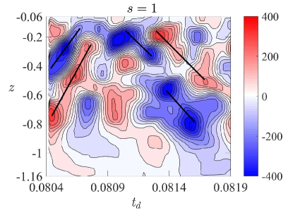
(a)

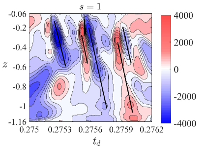
(b)

Figure 9: Contour plots of $\dot{B_{z}}$ shown for two time intervals. (a) $t_{d}=0.063-0.068$, $l\leq 42$. (b) $t_{d}=0.274-0.278$, $l\leq 31$. The cylindrical radius $s$ at which each plot is produced is given above the respective panel. The black lines indicate the direction of travel of the wave and their slope gives the measured group velocity. The dynamo parameters are $Ra=400$, $Pm=Pr=1$, $E=1.2\times 10^{-6}$. The estimated group velocity of the fast and slow MAC waves ($U_{f}$ and $U_{s}$ respectively) and the measured group velocity $U_{g,z}$ are given in table 4.

The contour plots of the time variation of the magnetic field $\dot{B}_{z}$ indicate that slow MAC wave motions are dominant even at early times when the field is weak (figure 9(a)). The measured group velocity $U_{g,z}$ is in fair agreement with the estimated slow wave velocity $U_{s}$ while the fast wave velocity $U_{f}$ is $O(10^{2})$ higher (table 4). (Here, the mean wavenumbers used for the theoretical estimate are those of the magnetic field.) This interesting distinction between the wave motions of the flow and field is well explained by Sreenivasan and Maurya (2021), who found that the induced magnetic field preferentially propagates as slow MAC waves for a wide range of $\omega_{M}/\omega_{C}\ll 1$ to $\sim 1$.

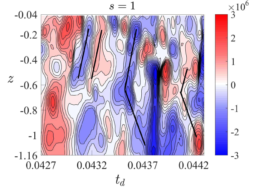
(a)

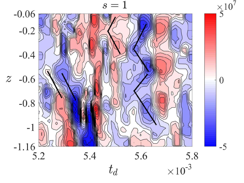
(b)

Figure 10: (a) Contour plot of $\dot{u_{z}}$ at for $l\leq 40$ and the parameters $E=1.2\times 10^{-5}$, $Ra=2000$, $Pr=Pm=5$. (b) $\dot{u_{z}}$ for $l\leq 46$ and the parameters $E=1.2\times 10^{-5}$, $Ra=15000$, $Pr=Pm=5$. The cylindrical radius $s$ at which each plot is produced is given above the respective panel. The black lines indicate the direction of travel of the wave and their slope gives the measured group velocity. The estimated group velocity of the fast and slow MAC waves ($U_{f}$ and $U_{s}$ respectively) and the measured group velocity $U_{g,z}$ are given in table 4.

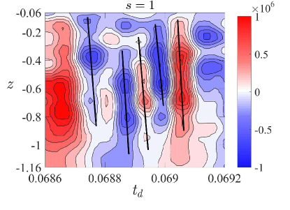
(a)

Figure 11: Contour plot of $\dot{u_{z}}$ for the scales $l\leq 42$ in a kinematic dynamo simulation with the parameters $E=1.2\times 10^{-6}$, $Ra=400$, $Pm=Pr=1$. The black lines indicate the direction of travel of the wave and their slope gives the measured group velocity. Similar plots are obtained for any time window in the simulation. The estimated group velocity of the fast and slow MAC waves ($U_{f}$ and $U_{s}$ respectively) and the measured group velocity $U_{g,z}$ are given in table 4.

The signature of the slow waves in the energy-containing scales is also visible in strongly driven dipolar dynamos (figure 10). As the intensity of the self-generated field increases with increased forcing, the range of azimuthal wavenumbers $m$ over which $|\omega_{C}|>|\omega_{M}|$ narrows down considerably (table 4). Consequently, the generation of helicity due to the slow MAC waves is weakened, which can explain why the axial dipole field $B^{P}_{10}$ diminishes in strength with increased forcing (table 1). There is, however, a growing dominance of fast waves in the large scales, which does not contribute to dipole field generation. At lower Ekman number $E$, one would expect the MAC wave window to widen as $|\omega_{C}|$ increases relative to $|\omega_{M}|$. The low-$E$ regime of Earth’s outer core would thus support the axial dipole in strongly driven convection. Finally, we note that only linear inertial waves are produced in kinematic dynamo simulations which produce multipolar fields (figure 11 and case (ix) in table 4).

Buoyancy-induced inertial waves have been found in dynamo simulations though group velocity measurements (Ranjan et al., 2018). The present study has shown that slow MAC wave motions are measurable only when large scales of $l\leq l_{E}$ are considered. Within this range, the slow waves are predominantly generated in the MAC wave window, where $|\omega_{C}|>|\omega_{M}|>|\omega_{A}|$. To identify the scales where fast and slow MAC waves are active and distinguishable from each other, a scale-dependent analysis of the dynamo spectrum is essential.

Table 4: Summary of the data for MAC wave identification in the dynamo simulations. Scales given by $l\leq l_{E}$, where $l_{E}$ is the mean harmonic degree of energy injection, are considered in each case. The sampling frequency $\omega_{n}$ is chosen to ensure that the fast MAC waves are not missed in the measurement of group velocity. The values of $\omega_{M}^{2}$, $\omega_{A}^{2}$ and $\omega_{C}^{2}$ are calculated from (7) using the mean wavenumbers $\bar{m}$, $\bar{k}_{s}$ and $\bar{k}_{z}$. The measured group velocity in the $z$ direction ($U_{g,z}$) may be compared with the estimated fast ($U_{f}$) or slow ($U_{s}$) MAC wave velocity, as appropriate. ^∗Case (ix) is a kinematic dynamo simulation, which does not produce an axial dipole.

S.No.	$E$	$Ra$	Fig. no.	$\omega_{n}$$(\times 10^{5})$	Scales	$\bar{m}$	$\bar{k}_{s}$	$\bar{k}_{z}$	$\omega_{M}^{2}$$(\times 10^{9})$	$-\omega_{A}^{2}$$(\times 10^{9})$	$\omega_{C}^{2}$$(\times 10^{9})$	$U_{s}$	$U_{f}$	$U_{g,z}$
(i)	$1.2\times 10^{-6}$	$400$	7(a)	6.67	$l\leq 42$	$12$	$3.14$	$2.51$	$0.28$	$0.31$	$27.3$	$-$	$63149$	$57333$
(ii)			7(b)	6.67	$l\leq 36$	$20$	$3.13$	$2.51$	$1.1$	$0.33$	$10.5$	$2741$	$37434$	$2133$
(iii)			7(c)	5	$l\leq 31$	$10$	$3.05$	$2.17$	$2.79$	$0.31$	$28.6$	$4054$	$70749$	$4864$
(iv)			7(d)	5	$l\leq 31$	$10$	$3.05$	$2.11$	$3.66$	$0.31$	$27.1$	$5295$	$69765$	$6534$
(v)			9(a)	6.67	$l\leq 42$	$11$	$3.61$	$1.43$	$3.9$	$0.30$	$10.4$	$780$	$69137$	$966$
(vi)			9(b)	5	$l\leq 31$	$9$	$3.45$	$1.67$	$1.68$	$0.29$	$23.4$	$3625$	$78988$	$3750$
(vii)	$1.2\times 10^{-5}$	$2000$	10(a)	3.33	$l\leq 40$	$12$	$4.24$	$2.34$	$4.25$	$0.74$	$5.7$	$5071$	$25957$	$6100$
(viii)	$1.2\times 10^{-5}$	$15000$	10(b)	1.67	$l\leq 46$	$4$	$4.78$	$2.63$	$12.9$	$0.36$	$31.2$	$4856$	$43656$	$5187$
(ix)∗	$1.2\times 10^{-6}$	$400$	11	10	$l\leq 42$	$16$	$4.95$	$2.64$	-	-	$1.68$	-	$48396$	$55000$

5.1 Non-axisymmetric Alfvén waves

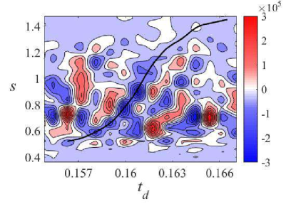
(a)

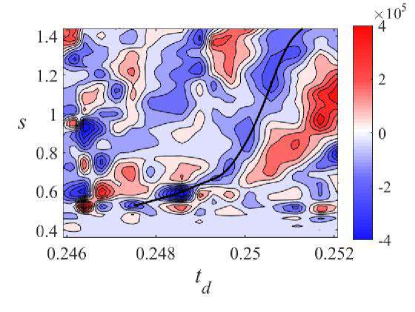
(b)

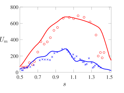
(c)

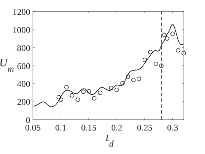
(d)

Figure 12: (a) and (b) Contour plots of $\dot{u}_{z}$ for two time intervals for the large scales of $l\leq 31$. The group velocity of the waves is measured from the slope of the black line. (c) Comparison of estimated (theoretical) and measured velocities at each instant of time for the time intervals in (a) and (b), shown in blue and red respectively. The solid line gives the estimated velocity and symbols represent the measured values. (d) Comparison of peak velocities measured in the simulations at various points in the equatorial cross-sections. The symbols show the peak measured velocity of $\dot{u}_{z}$ while the black line shows the estimated velocity. The black dashed line shows the dipole formation time. Parameters are $Ra=400$, $Pm=Pr=1$, $E=1.2\times 10^{-6}$. The group velocity is estimated using the local value of $B_{s}$ averaged over $z$.

The generation of MAC waves in the dynamo is accompanied by non-axisymmetric waves along the cylindrical radius whose group velocity matches with that of Alfvén waves. The frequencies of waves that propagate orthogonal to the axis of rotation – obtained by letting $\omega_{C}=0$ in equations (8) and (9) – would be Alfvénic for strong-field dynamos where $|\omega_{C}|>|\omega_{M}|>|\omega_{A}|$. In the dynamo simulation at $E=1.2\times 10^{-6}$ and $Ra=400$, coherent radial motion with estimated Alfvén velocities is only noted after diffusion time $t_{d}\approx 0.1$. Since slow MAC waves are first excited at $t_{d}\approx 0.04$ during the growth phase of the dynamo (figure 6(b)), it is reasonable to suppose that the Alfvén waves exist as the degenerate form of the MAC waves. In the contour plots of $\dot{u_{z}}$ given in figure 12 (a) and (b), the wave velocity is the slope measured over small time windows. Figure 12 (c) shows the variation of the wave velocity with cylindrical radius $s$ for the two time intervals in (a) and (b), with the earlier interval showing lower velocity. The peak wave velocities measured throughout the simulation show a good agreement with the Alfvén velocities calculated from the $z$-averaged local value of $B_{s}^{2}$. The increase in the measured wave velocity with the increasing intensity of $B_{s}$ in time is evident in figure 12 (d). The waves slow down at the outer boundaries where the field intensity is weak. As we see below, the non-axisymmetric waves explain the growth of $u_{z}$ in the $s$ direction, an essential process in dipole formation from a seed magnetic field.

6 Termwise contributions to the axial dipole

To understand how wave motion influences the formation of the axial dipole field through the magnetic induction equation, we look at stretching and advection terms in this equation which dominantly influence the dipole. The relative positive and negative contributions to the dipole are given by

$$\frac{\int_{V}|\bm{B}^{P}_{10}|\,\,[\,.\,]\,dV}{\Gamma^{P}_{10}},$$ (13)

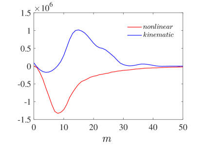
Figure 13: Spectral distribution of the contribution to the axial dipole energy from the term $(B_{\phi}/s)\partial u_{s}/\partial\phi$ for nonlinear and kinematic simulations at $E=1.2\times 10^{-5}$ and $Pm=Pr=5$. The nonlinear result is obtained from the saturated state at $Ra=220$ whereas the kinematic result is from a snapshot at $Ra=140$.

where $\Gamma^{P}_{10}$ is defined in equation (11) and the quantity within square brackets $[\,.\,]$ would be one of terms given in table 5. In cylindrical polar coordinates, the two terms which make the highest positive contribution to the axial dipole are $B_{s}\partial u_{z}/\partial s$ and $B_{s}\partial u_{s}/\partial s$. A significant positive contribution is also noted for the term $B_{z}\partial u_{z}/\partial z$. The terms $B_{s}\partial u_{s}/\partial s$ and $B_{z}\partial u_{z}/\partial z$ are related to the production of current coils in dynamo simulations (Kageyama et al., 2008; Takahashi and Shimizu, 2012). The term $B_{s}\partial u_{z}/\partial s$ represents axial field generation due to shear of axial ($z$) flow in the radial ($s$) direction. This process would be influential during the growth phase of the nonlinear dynamo, where columnar convection is excited through slow MAC wave motions. In table 5, the termwise contributions to the dipole in nonlinear simulations are compared with those in a kinematic simulation at $E=1.2\times 10^{-5}$ and $Ra=140$, which also produces an axial dipole. Kinematic simulations at higher $Ra$ do not produce an axial dipole (Sreenivasan and Kar, 2018), and hence cannot be used for comparison with the nonlinear simulations. Even in the absence of slow wave motion, the term $B_{s}\partial u_{z}/\partial s$ contributes positively to dipole growth in the kinematic dynamo due to the growth of $B_{s}$. Surprisingly, the toroidal–poloidal field conversion via the term $(B_{\phi}/s)\partial u_{s}/\partial{\phi}$ – a dominant process in the kinematic simulation – is absent in the nonlinear simulation (table 5). In fact, $B^{s}_{10}$, the axial dipole part of the radial field component, is negatively correlated with $(B_{\phi}/s)\partial u_{s}/\partial{\phi}$ in the nonlinear simulation (figure 13). The contribution of this term to the overall poloidal field is, however, positive, which suggests that the classical alpha effect (Moffatt, 1978) is still influential in generating the full poloidal field from the toroidal field. We also note from table 5 that the dipole contributions of the terms $B_{z}\partial u_{z}/\partial z$, $B_{s}\partial u_{s}/\partial s$ and $B_{z}\partial u_{s}/\partial z$ are all oppositely signed in the nonlinear and kinematic simulations.

The advection terms influenced by wave motion also make influential contributions to the axial dipole. The terms $-u_{z}\partial B_{z}/\partial z$ and $-u_{s}\partial B_{s}/\partial s$ increase preferentially in the growth phase of the nonlinear dynamo and are dominant positive contributors to the dipole.

Table 5: Relative contribution (in per cent) to the axial dipole by the dominant stretching and advection terms in the magnetic induction equation, calculated from the ratio (13). The values are evaluated up to dipole formation time and averaged for the energy-containing (large) scales in the nonlinear simulations. The entire range of scales is considered for the kinematic simulation, marked by the superscript *.

$E$, $Ra$
$1.2\times 10^{-6},400$	$B_{s}\partial u_{s}/\partial s$	$B_{s}\partial u_{z}/\partial s$	$B_{z}\partial u_{z}/\partial z$	$B_{z}\partial u_{s}/\partial z$	$(B_{\phi}/s)\partial u_{z}/\partial\phi$	$(B_{\phi}/{s})\partial u_{s}/\partial\phi$
	57.6	52.17	31.04	-38.75	-44.79	-59.4
$1.2\times 10^{-5},500$	$B_{s}\partial u_{s}/\partial s$	$B_{s}\partial u_{z}/\partial s$	$B_{z}\partial u_{z}/\partial z$	$B_{z}\partial u_{s}/\partial z$	$(B_{\phi}/s)\partial u_{z}/\partial\phi$	$(B_{\phi}/{s})\partial u_{s}/\partial\phi$
	50.8	43.5	36.9	-33.84	-46.7	-49.5
$1.2\times 10^{-5},2000$	$B_{s}\partial u_{s}/\partial s$	$B_{s}\partial u_{z}/\partial s$	$B_{z}\partial u_{z}/\partial z$	$B_{z}\partial u_{s}/\partial z$	$(B_{\phi}/s)\partial u_{s}/\partial\phi$	$(B_{\phi}/s)\partial u_{s}/\partial\phi$
	55.01	48.7	44.4	-39.1	-44.05	-61.4
∗$1.2\times 10^{-5},140$	$B_{s}\partial u_{z}/\partial s$	$(B_{\phi}/{s})\partial u_{s}/\partial\phi$	$B_{z}\partial u_{s}/\partial z$	$B_{z}\partial u_{z}/\partial z$	$B_{s}\partial u_{s}/\partial s$	$(B_{\phi}/s)\partial u_{z}/\partial\phi$
	131.2	88.61	42.78	-49.94	-88.3	-102.1
$1.2\times 10^{-6},400$	$-u_{z}\partial B_{z}/\partial z$	$-u_{s}\partial B_{s}/\partial s$	$-u_{z}\partial B_{s}{\partial z}$	$-u_{z}\partial B_{s}/\partial z$	$-(u_{\phi}/{s})\partial B_{z}/\partial\phi$	$-(u_{\phi}/{s})\partial B_{s}/\partial\phi$
	44.95	40.13	27.50	-45.48	-49.91	-51.2
$1.2\times 10^{-5},500$	$-u_{z}\partial B_{z}/\partial z$	$-u_{s}\partial B_{s}/\partial s$	$-u_{z}\partial B_{s}/\partial z$	$-(u_{\phi}/s)\partial B_{s}/\partial\phi$	$-(u_{\phi}/s)\partial B_{z}/\partial\phi$	$-u_{s}\partial B_{z}/\partial s$
	52.63	41.98	30.02	-43.10	-48.61	-50.09
$1.2\times 10^{-5},2000$	$-u_{z}\partial B_{z}/\partial z$	$-u_{s}\partial B_{s}/\partial s$	$-u_{z}\partial B_{s}/\partial z$	$-(u_{\phi}/s)\partial B_{s}/\partial\phi$	$-u_{s}B_{z}/\partial s$	$-(u_{\phi}/s)\partial B_{z}/\partial\phi$
	43.9	31.5	24.5	-34.57	-45.61	-47.18
∗$1.2\times 10^{-5},140$	$-(u_{\phi}/{s})\partial B_{z}/\partial\phi$	$-u_{s}\partial B_{s}/\partial s$	$-u_{z}\partial B_{z}/\partial z$	$-u_{z}\partial B_{s}/\partial z$	$-u_{s}\partial B_{z}/\partial s$	$-(u_{\phi}/s)\partial B_{s}/\partial\phi$
	113.25	87.34	22.51	-40.59	-63.1	-118.6

7 Concluding remarks

The formation of the axial dipole field in a planetary dynamo is strongly dependent not only on the rotation of the planet but also the self-generated magnetic field within its core. As suggested by earlier studies (Sreenivasan and Jones, 2011; Sreenivasan and Kar, 2018), the role of the magnetic field in dipole formation is well understood from dynamo models that follow the evolution of the magnetic field from a small seed state. At early times of evolution, the fast MAC waves, whose frequency is close to that of linear inertial waves, are abundantly present. As the field exceeds a threshold, marked by $|\omega_{M}|>|\omega_{A}|$, slow MAC waves appear; however, it is only when the field is strong enough to have $|\omega_{M}/\omega_{C}|\sim$ 0.1 that the slow waves have a dominant presence in the dynamo (table 3 and figure 7(c)). The value of $|\omega_{M}|$ here must be based on the peak rather than the root mean square value of the field, for the so-called MAC wave window that satisfies the inequality $|\omega_{C}|>|\omega_{M}|>|\omega_{A}|$ does not otherwise exist in the energy-containing scales of the dynamo. A recent study on the evolution of isolated blobs subject to this inequality (Sreenivasan and Maurya, 2021) indicates that the local Elsasser number,

$$\varLambda\sim\left(\dfrac{\omega_{M}^{2}}{\omega_{C}\omega_{\eta}}\right)_{0},$$

would likely be $O(10^{2})$ for parity between the intensities of fast and slow wave motions. The subscript ’0’ here refers to the “isotropic” state of the blob that is released into the flow by buoyancy. In other words, the leading-order slow MAC wave frequency $\omega_{s}$ would be $O(10^{2})$ times the magnetic diffusion frequency $\omega_{\eta}$. The peak value of $\varLambda$ in simulations at $E\sim 10^{-6}$ vary from $O(10^{1})$–$O(10^{2})$ as the dynamo field increases towards the saturated state (figure 14). The instantaneous value of $\omega_{s}/\omega_{\eta}$ is higher than $\varLambda$ due to the anisotropy of the convection as blobs elongate to form columns aligned with the axis of rotation. We anticipate that simulations at lower $E$ would give $\varLambda$ of $O(10^{2})$ for a wider range of $|\omega_{M}/\omega_{C}|\sim$ 0.1 than in this study. The large local value of $\varLambda$ supports the localized excitation of slow magnetostrophic waves at several points in the large scales of spherical harmonic degree $l\leq l_{E}$, even as a global geostrophic balance exists at these scales (e.g. Aurnou and King, 2017). The generation of dynamo helicity – of the same order of magnitude as the nonmagnetic helicity (figure 3(a) and (b)) – is consistent with the excitation of the slow waves at these scales.

An interesting aspect of dipole field generation through wave motion is that of poloidal–poloidal field conversion via the term $B_{s}\partial u_{z}/\partial s$ in the induction equation. While this term contributes to dipole formation at low $Ra$ in kinematic dynamos through the monotonic increase of $B_{s}$, its effect is more pronounced in the nonlinear dynamo over a wide range of $Ra$, where the generation of radial gradients of $u_{z}$ happens through the radial propagation of columnar vortices at the Alfvén speed. The twisting of the toroidal field by the radial motion makes a strongly positive contribution to the poloidal dipole field in the kinematic dynamo, whereas it extracts energy from the dipole field in the nonlinear dynamo (figure 13).

Since the present study has largely focused on the formation of the axial dipole through magnetostrophic waves, moderately driven dynamos where $|\omega_{A}|<|\omega_{M}|$ have been analysed in detail. This regime is motivated in part by the thermally convecting core of early Earth, which would have produced an axial dipole from a chaotic multipolar field (Sreenivasan and Kar, 2018). The stronger self-generated field that accompanies stronger forcing in numerical dynamos narrows down the MAC wave window in the large scales, although this would not shut down the MAC waves in the rapidly rotating, low-$E$ core. If forcing is so strong that $|\omega_{A}|\sim|\omega_{M}|$, then the slow MAC wave frequency would be considerably attenuated. Consequently, the helicity associated with the slow waves would diminish relative to that of the fast waves, which are practically unaffected by the strength of forcing. If geomagnetic reversals are indeed buoyancy-driven (Sreenivasan et al., 2014), then the attenuation of the slow waves should provide a useful constraint on the parameter space that admits reversals.

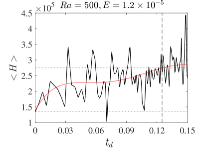
(a)

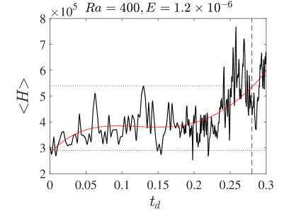
(b)

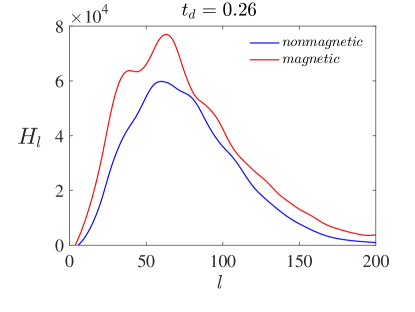
(c)

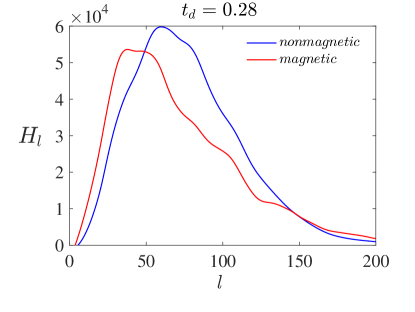
(d)

Figure 3: (a) & (b) Sum of the axial ($z$) and radial ($s$) helicity $<\!\!H\!\!>$ for the lower half of the spherical shell, plotted against time (measured in units of the magnetic diffusion time $t_{d}$). The scales considered are $l\leq 23$ for (a) and $l\leq 31$ for (b). The dynamo parameters are $Ra=500$, $Pm=Pr=5$, $E=1.2\times 10^{-5}$ for (a) and $Ra=400$, $Pm=Pr=1$, $E=1.2\times 10^{-6}$ for (b). The dashed vertical line indicates dipole formation time. (c) & (d) Distribution of helicity over spherical harmonic degree at two times near dipole formation for the simulation in (b).

References

- Acheson and Hide (1973) Acheson, D. J., Hide, R., 1973. Hydromagnetics of rotating fluids. Rep. Prog. Phys. 36, 159.
- Aubert and Finlay (2019) Aubert, J., Finlay, C. C., 2019. Geomagnetic jerks and rapid hydromagnetic waves focusing at earth’s core surface. Nature Geoscience 12 (5), 393–398.
- Aubert et al. (2017) Aubert, J., Gastine, T., Fournier, A., 2017. Spherical convective dynamos in the rapidly rotating asymptotic regime. J. Fluid Mech. 813, 558–593.
- Aurnou and King (2017) Aurnou, J. M., King, E. M., Mar 2017. The cross-over to magnetostrophic convection in planetary dynamo systems. Proc. R. Soc. A. 473 (2199), 20160731.
- Bardsley and Davidson (2016) Bardsley, O. P., Davidson, P. A., 2016. Inertial–alfvén waves as columnar helices in planetary cores. J. Fluid Mech. 805, R2.
- Braginsky (1967) Braginsky, S. I., 1967. Magnetic waves in the Earth’s core. Geomagn. Aeron. 7, 851–859.
- Braginsky and Roberts (1995) Braginsky, S. I., Roberts, P. H., 1995. Equations governing convection in Earth’s core and the geodynamo. Geophys. Astrophys. Fluid Dyn. 79, 1–97.
- Buffett and Bloxham (2002) Buffett, B., Bloxham, J., 2002. Energetics of numerical geodynamo models. Geophysical journal international 149 (1), 211–224.
- Buffett et al. (2016) Buffett, B., Knezek, N., Holme, R., 2016. Evidence for MAC waves at the top of Earth’s core and implications for variations in length of day. Geophys. J. Int. 204 (3), 1789–1800.
- Busse et al. (2007) Busse, F., Dormy, E., Simitev, R., Soward, A., 2007. Dynamics of rotating fluids. In: Dormy, E., Soward, A. M. (Eds.), Mathematical Aspects of Natural Dynamos. Vol. 13 of The Fluid Mechanics of Astrophysics and Geophysics. CRC Press, pp. 119–198.
- Busse (1976) Busse, F. H., 1976. Generation of planetary magnetism by convection. Phys. Earth Planet. Inter. 12, 350–358.
- Christensen and Aubert (2006) Christensen, U. R., Aubert, J., 2006. Scaling properties of convection-driven dynamos in rotating spherical shells and application to planetary magnetic fields. Geophys. J. Int. 166 (1), 97–114.
- Hori et al. (2015) Hori, K., Jones, C., Teed, R., 2015. Slow magnetic rossby waves in the earth’s core. Geophysical Research Letters 42 (16), 6622–6629.
- Jault (2008) Jault, D., 2008. Axial invariance of rapidly varying diffusionless motions in the Earth’s core interior. Phys. Earth Planet. Inter. 166, 67–76.
- Kageyama et al. (2008) Kageyama, A., Miyagoshi, T., Sato, T., Aug 2008. Formation of current coils in geodynamo simulations. Nature 454, 1106–1109.
- Kageyama and Sato (1997) Kageyama, A., Sato, T., 1997. Generation mechanism of a dipole field by a magnetohydrodynamic dynamo. Physical Review E 55 (4), 4617.
- Kono and Roberts (2002) Kono, M., Roberts, P. H., 2002. Recent geodynamo simulations and observations of the geomagnetic field. Rev. Geophys. 40, 101–113.
- Moffatt (1978) Moffatt, H. K., 1978. Magnetic Field Generation in Electrically Conducting Fluids. Cambridge University Press.
- Olson et al. (1999) Olson, P., Christensen, U., Glatzmaier, G. A., 1999. Numerical modeling of the geodynamo: mechanisms of field generation and equilibration. J. Geophs. Res. Solid Earth 104 (B5), 10383–10404.
- Peña et al. (2018) Peña, D., Amit, H., Pinheiro, K. J., Dec 2018. Deep magnetic field stretching in numerical dynamos. Prog. Earth Planet. Sci. 5 (1), 1–23.
- Ranjan et al. (2018) Ranjan, A., Davidson, P. A., Christensen, U. R., Wicht, J., 2018. Internally driven inertial waves in geodynamo simulations. Geophys. J. Int. 213 (2), 1281–1295.
- Ranjan et al. (2020) Ranjan, A., Davidson, P. A., Christensen, U. R., Wicht, J., 2020. On the generation and segregation of helicity in geodynamo simulations. Geophys. J. Int. 221 (2), 741–757.
- Roberts and Zhang (2000) Roberts, P. H., Zhang, K., 2000. Thermal generation of Alfvén waves in oscillatory magnetoconvection. J. Fluid Mech. 420, 201–223.
- Schaeffer et al. (2017) Schaeffer, N., Jault, D., Nataf, H.-C., Fournier, A., 2017. Turbulent geodynamo simulations: a leap towards Earth’s core. Geophys. J. Int. 211, 1–29.
- Sreenivasan and Gopinath (2017) Sreenivasan, B., Gopinath, V., Jul 2017. Confinement of rotating convection by a laterally varying magnetic field. J. Fluid Mech. 822, 590–616.
- Sreenivasan and Jones (2006) Sreenivasan, B., Jones, C. A., 2006. The role of inertia in the evolution of spherical dynamos. Geophys. J. Int. 164 (2), 467–476.
- Sreenivasan and Jones (2011) Sreenivasan, B., Jones, C. A., 2011. Helicity generation and subcritical behaviour in rapidly rotating dynamos. J. Fluid Mech. 688, 5–30.
- Sreenivasan and Kar (2018) Sreenivasan, B., Kar, S., 2018. Scale dependence of kinetic helicity and selection of the axial dipole in rapidly rotating dynamos. Phys. Rev. Fluids 3 (9), 093801.
- Sreenivasan and Maurya (2021) Sreenivasan, B., Maurya, G., 2021. Evolution of forced magnetohydrodynamic waves in a stratified fluid. J. Fluid Mech. 922, A32.
- Sreenivasan et al. (2014) Sreenivasan, B., Sahoo, S., Dhama, G., 2014. The role of buoyancy in polarity reversals of the geodynamo. Geophys. J. Int. 199, 1698–1708.
- Takahashi and Shimizu (2012) Takahashi, F., Shimizu, H., 2012. A detailed analysis of a dynamo mechanism in a rapidly rotating spherical shell. Journal of Fluid Mechanics 701, 228–250.
- Teed et al. (2014) Teed, R. J., Jones, C. A., Tobias, S. M., 2014. The dynamics and excitation of torsional waves in geodynamo simulations. Geophys. J. Int. 196 (2), 724–735.
- Wicht and Christensen (2010) Wicht, J., Christensen, U. R., 2010. Torsional oscillations in dynamo simulations. Geophys. J. Int. 181 (3), 1367–1380.
- Willis et al. (2007) Willis, A. P., Sreenivasan, B., Gubbins, D., 2007. Thermal core-mantle interaction: Exploring regimes for ‘locked’ dynamo action. Phys. Earth Planet. Inter. 165, 83–92.