Nonparametric extensions of randomized
response for private confidence sets

Abstract

This work derives methods for performing nonparametric, nonasymptotic statistical inference for population means under the constraint of local differential privacy (LDP). Given bounded observations $(X_{1},\dots,X_{n})$ with mean $\mu^{\star}$ that are privatized into $(Z_{1},\dots,Z_{n})$, we present confidence intervals (CI) and time-uniform confidence sequences (CS) for $\mu^{\star}$ when only given access to the privatized data. To achieve this, we introduce a nonparametric and sequentially interactive generalization of Warner’s famous “randomized response” mechanism, satisfying LDP for arbitrary bounded random variables, and then provide CIs and CSs for their means given access to the resulting privatized observations. For example, our results yield private analogues of Hoeffding’s inequality in both fixed-time and time-uniform regimes. We extend these Hoeffding-type CSs to capture time-varying (non-stationary) means, and conclude by illustrating how these methods can be used to conduct private online A/B tests.

toc

1 Introduction

It is easier than ever for mobile apps and web browsers to collect massive amounts of sensitive data about individuals. Differential privacy (DP) provides a framework that leverages statistical noise to limit the risk of sensitive information disclosure [28]. The goal of private data analysis is to extract meaningful population-level information from the data (whether in the form of machine learning model training, statistical inference, etc.) while preserving the privacy of individuals via DP. In particular, this paper will focus on statistical inference (e.g. confidence intervals and $p$-values) for population means under DP constraints.

As motivating examples, suppose a city wishes to survey households to calculate the approval rating of their mayor, or an IT company aims to understand whether a redesigned homepage will lead to the average user spending more time on it. Both problems can be framed as estimating the mean of some (potentially large) population, but it may be infeasible to query every single household or all possible website users. Fortunately, a sample mean can still be used to estimate the population mean with some degree of precision. For example, a city may randomly choose households to query, or the technology company may show 10% of users the redesigned webpage at random. This is often referred to as “A/B testing”, and we expand on this application under privacy constraints in Section 4. When making decisions, however, it is crucial to both calculate sample means and quantify the uncertainty in those estimates (e.g. using confidence intervals, reviewed in Section 1.2). However, calculating confidence intervals under local differential privacy constraints (defined in Section 1.1) poses a unique statistical challenge, because these intervals must incorporate both the uncertainty introduced from random sampling and from the privacy mechanism. This paper studies and provides a nonparametric solution to precisely this challenge.

1.1 Background I: Local Differential Privacy

There are two main models of privacy within the DP framework: central and local DP (LDP) [28, 47, 27]. The former involves a centralized data aggregator that is trusted with constructing privatized output from raw data, while the latter performs privatization at the “local” or “personal” level (e.g. on an individual’s smartphone before leaving the device) so that trust need not be placed in any data collector. Both models have their advantages and disadvantages: LDP is a more restrictive model of privacy and thus in general requires more noise to be added. On the other hand, the stronger privacy guarantees that do not require a trusted central aggregator make LDP an attractive framework in practice. This paper deals exclusively with LDP.

Making our setup more precise, suppose $X_{1},X_{2},\dots$ is a (potentially infinite) sequence of $[0,1]$-valued random variables. We could instead have assumed boundedness on any known interval $[a,b]$ since we can always translate and scale the interval to $[0,1]$ via the transformation $x\mapsto(x-a)/(b-a)$. We will refer to $(X_{t})_{{t}={1}}^{\infty}$ as the “raw” or “sensitive” data that are yet to be privatized. Following the notation of Duchi et al. [24] the privatized views $Z_{1},Z_{2},\dots$ of $X_{1},X_{2},\dots$, respectively are generated by a sequence of conditional distributions $Q_{1},Q_{2},\dots$ which we refer to as the privacy mechanism. Throughout this paper, we will allow this privacy mechanism to be sequentially interactive, meaning that the distribution $Q_{i}$ of $Z_{i}$ may depend on the past privatized observations $Z_{1}^{i-1}:=(Z_{1},\dots,Z_{i-1})$ [24]. In other words, the privatized view $Z_{i}$ of $X_{i}$ has a conditional distribution $Q_{i}(\cdot\mid X_{i}=x,Z_{1}^{i-1}=z_{1}^{i-1})$. Following Duchi et al. [24, 26] we say that $Q_{i}$ satisfies $\varepsilon$-local differential privacy if for all $z_{1},\dots,z_{i-1}\in[0,1]$ and $x,\widetilde{x}\in[0,1]$, the following likelihood ratio is uniformly bounded:

$$\small\sup_{z\in[0,1]}\frac{q_{i}(z\mid X_{i}=x,Z_{1}^{i-1}=z_{1}^{i-1})}{q_{i}(z\mid X_{i}=\widetilde{x},Z_{1}^{i-1}=z_{1}^{i-1})}\leq\exp\{\varepsilon\},$$ (1)

where $q_{i}$ is the density (or Radon-Nikodym derivative) of $Q_{i}$ with respect to some dominating measure. In the non-interactive case where the dependence on $Z_{1}^{i-1}$ is dropped, (1) simplifies to the usual $\varepsilon$-LDP definition [27]. To put $\varepsilon>0$ in a real-world context, Apple uses privacy levels in the range of $\varepsilon\in\{2,4,8\}$ on macOS and iOS devices for various $\varepsilon$-LDP data collection tasks, including health data type usage, emoji suggestions, and lookup hints [7]. See Fig. 1 to intuit how $\varepsilon$ affects the widths of confidence intervals that we develop. Next, we review time-uniform confidence sequences and how they differ from fixed-time confidence intervals.

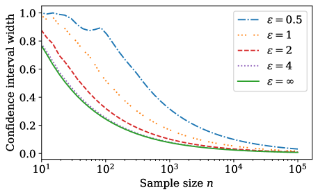
Figure 1: Widths of private 90%-CIs for the mean of a uniform distribution using our private Hoeffding CI given in (11) for various levels of $\varepsilon$ ranging from $\varepsilon=0.5$ (very private) to $\varepsilon=\infty$ (no privacy). Unsurprisingly, less privacy leads to sharper inference, but notice that inference is still practical, especially for $\varepsilon\geq 2$. For context, Apple uses $\varepsilon\in\{2,4,8\}$ for various data collection tasks on iPhones [7]. At these levels of privacy, our CIs perform nearly as well as — and are in some cases indistinguishable from — the non-private Hoeffding CI.

1.2 Background II: Confidence Sequences

One of the most fundamental tasks in statistical inference is the derivation of confidence intervals (CI) for a parameter of interest $\mu^{\star}\in\mathbb{R}$ (e.g. mean, variance, treatment effect, etc.). Given data $X_{1},\dots,X_{n}$, the interval $\dot{C}_{n}\equiv C(X_{1},\dots,X_{n})$ is said to be a $(1-\alpha)$-CI for $\mu^{\star}$ if

$$\small\mathbb{P}(\mu^{\star}\notin\dot{C}_{n})\leq\alpha,$$ (2)

where $\alpha\in(0,1)$ is a prespecified error tolerance. Notice that (2) is a “pointwise” or “fixed-time” statement, meaning that it only holds for a single fixed sample size $n$.

The “time-uniform” analogue of CIs are so-called confidence sequences (CS) — sequences of confidence intervals that are uniformly valid over a (potentially infinite) time horizon [20, 54]. We say that the sequence $(\bar{C}_{t})_{{t}={1}}^{\infty}$ is a $(1-\alpha)$-CS for $\mu^{\star}$ if

$$\small\mathbb{P}(\exists t\geq 1:\mu^{\star}\notin\bar{C}_{t})\leq\alpha.$$ (3)

The guarantee (3) has important implications for data analysis, giving practitioners the ability to (a) update inferences as new data become available, (b) continuously monitor studies without any statistical penalties for “peeking”, and (c) make decisions based on valid inferences at arbitrary stopping times: for any stopping time $\tau$, $\mathbb{P}(\mu^{\star}\notin\bar{C}_{\tau})\leq\alpha$.

1.3 Contributions and Outline

Our primary contributions are threefold: (a) a new privacy mechanism, (b) CIs, and (c) time-uniform CSs.

1. We introduce NPRR — a sequentially interactive, nonparametric generalization of Warner’s randomized response [67] for bounded data (Section 2).

2. We derive several CIs for the mean of bounded random variables that are privatized by NPRR (Section 3). We believe Section 3 introduces the first private nonparametric CIs for means of bounded random variables.

3. We derive time-uniform CSs for the mean of bounded random variables that are privatized by NPRR, enabling private nonparametric sequential inference (Section 3.3). We also introduce a CS that is able to capture means that change over time under no stationarity conditions on the time-varying means (Section 3.4). We believe Sections 3.3 and 3.4 are the first private nonparametric CSs in the DP literature.

Furthermore, we show how all of the aforementioned techniques can be used to conduct private online A/B tests (Section 4). Finally, Section 5 summarizes our findings and discusses some additional results whose details can be found in the appendix. A Python package implementing our methods as well as code to reproduce the figures can be found on GitHub at github.com/WannabeSmith/nprr.

1.4 Related Work

The literature on differentially private statistical inference is rich, including nonparametric estimation rates [68, 24, 25, 26, 45, 16, 4], parametric hypothesis testing and confidence intervals [61, 66, 32, 9, 46, 17, 41, 30, 19], median estimation [22], independence testing [18], online convex optimization [42], and parametric sequential hypothesis testing [65]. A more detailed summary can be found in Section D.

The aforementioned works do not study the problem of private nonparametric confidence sets for population means. Prior work does exist on confidence intervals for the sample mean of the data [21, 63]. The most closely related work is that of Ding et al. [21, Section 2.1] who introduce the “1BitMean” mechanism which can be viewed as a special case of NPRR (Algorithm 2). They derive a private Hoeffding-type confidence interval for the sample mean of the data, but it is important to distinguish this from the more classical statistical task of population mean estimation. For example, if $X_{1},\dots,X_{n}$ are random variables drawn from a distribution with mean $\mu^{\star}$, then the population mean is $\mu^{\star}$, while the sample mean is $\widehat{\mu}_{n}:=\frac{1}{n}\sum_{i=1}^{n}X_{i}$. A private CI for $\mu^{\star}$ incorporates randomness from both the mechanism and the data, while a CI for $\widehat{\mu}_{n}$ incorporates randomness from the mechanism only. Neither is a special case of the other, and some of our techniques allow for the (sequential) estimation of sample means (see Section B.2 for details and explicit bounds) but this paper is primarily focused on the problem of private population mean estimation.

2 Extending Warner’s Randomized Response

Before introducing our nonparametric extension of randomized response, let us briefly review Warner’s classical randomized response mechanism as well as the Laplace mechanism, discuss their shortcomings, and introduce a new mechanism to remedy them.

Warner’s randomized response. When the raw data $(X_{t})_{{t}={1}}^{\infty}$ are binary, one of the oldest and simplest privacy mechanisms is Warner’s randomized response (RR) [67]. Warner’s RR was introduced decades before the very definition of DP, but was later shown to satisfy LDP by Dwork and Roth [27]. RR was introduced as a method to provide plausible deniability to subjects when answering sensitive survey questions [67], and proceeds as follows: when presented with a sensitive Yes/No question (e.g. “have you ever used illicit drugs?”), the subject flips a biased coin with $\mathbb{P}(\text{Heads})=r\in(0,1]$. If the coin comes up heads, then the subject answers truthfully; if tails, the subject answers “Yes” or “No” (encoded as 1 and 0, respectively) with equal probability 1/2. It is easy to see that this mechanism satisfies $\varepsilon$-LDP with $\varepsilon=\log(1+\frac{2r}{1-r})$ by bounding the likelihood ratio of the privatized response distributions: for any true response $x\in\{0,1\}$, let $q(z\mid X=x)=r\mathds{1}(z=x)+(1-r)/2$ denote the conditional probability mass function of its privatized view. Then for any $x,\widetilde{x}\in\{0,1\}$,

$$\small\sup_{z\in\{0,1\}}\frac{q(z\mid X=x)}{q(z\mid X=\widetilde{x})}\leq 1+\frac{2r}{1-r},$$ (4)

and hence RR satisfies $\varepsilon$-LDP with $\varepsilon=\log(1+\frac{2r}{1-r})$. In Section B.1, we show how one can derive a CI for the mean of Bernoulli random variables when they are privatized via RR, but as we will see in Section 3, this will be an immediate corollary of a more general result for bounded random variables (Theorem 4).

One downside of RR, however, is that it takes binary data as input. On the other hand, the famous Laplace mechanism satisfies $\varepsilon$-LDP for bounded data, including binary ones.

The Laplace mechanism. The Laplace mechanism appeared in the very same paper that introduced DP [28]. Algorithm 1 recalls the (sequentially interactive) Laplace mechanism [24].

Algorithm 1 Sequentially interactive Laplace mechanism

  for t = 1,2,… do

     Choose $\varepsilon_{t}$ based on $Z_{1}^{t-1}$.

     Generate $\mathcal{L}_{t}\sim\mathrm{Laplace}(1/\varepsilon_{t})$ 

     $Z_{t}\leftarrow X_{t}+\mathcal{L}_{t}$ 

  end for

It is well-known that $Z_{t}$ is (conditionally) $\varepsilon_{t}$-LDP (given $Z_{1}^{t-1}$) for each $t$ [28]. Section B.4 derives novel CIs and CSs for population means under the Laplace mechanism, but we omit them here for brevity as our new mechanism (to be introduced shortly) will yield better bounds.

Nonparametric randomized response (NPRR). Our mechanism “Nonparametric randomized response” (NPRR) serves as a sequentially interactive generalization of RR for arbitrary bounded data by combining stochastic rounding [11, 31, 39] with $k$-RR — a categorical but non-interactive generalization of Warner’s RR introduced by Kairouz et al. [43, 44], and also considered by Li et al. [49] under the name “Generalized Randomized Response”. Note that Kairouz et al. [43, 44] use $k$ to refer to the number of unique values that the input and output data can take on, which is $k=G+1$ in the case of Algorithm 2. NPRR is explicitly described in Algorithm 2, and its LDP guarantees are summarized in Theorem 1.

Algorithm 2 Nonparametric randomized response (NPRR)

  for $t=1,2,\dots$ do

     // Step 1: Discretize $X_{t}$ into $Y_{t}$ via stochastic rounding.

     Choose integer $G_{t}\geq 1$ based on $Z_{1}^{t-1}$ 

     $X_{t}^{\mathrm{ceil}}\leftarrow\lceil G_{t}X_{t}\rceil/G_{t}$, $X_{t}^{\mathrm{floor}}\leftarrow\lfloor G_{t}X_{t}\rfloor/G_{t}$  

     if $X_{t}^{\mathrm{ceil}}==X_{t}^{\mathrm{floor}}$ then

        $Y_{t}\leftarrow X_{t}$

     else

        Generate $Y_{t}\sim\begin{cases}X_{t}^{\mathrm{ceil}}&\text{w.p. }G_{t}\cdot(X_{t}-X_{t}^{\mathrm{floor}})\\ X_{t}^{\mathrm{floor}}&\text{w.p. }G_{t}\cdot(X_{t}^{\mathrm{ceil}}-X_{t})\end{cases}$  

     end if

     // Step 2: Privatize $Y_{t}$ into $Z_{t}$ via $k$-RR.

     Choose $r_{t}\in(0,1]$ based on $Z_{1}^{t-1}$ 

     Generate $\mathcal{U}_{t}\sim\mathrm{Unif}\left\{0,\frac{1}{G_{t}},\frac{2}{G_{t}},\dots,\frac{G_{t}}{G_{t}}\right\}$ 

     Generate $Z_{t}\sim\begin{cases}Y_{t}&\text{w.p. }r_{t}\\ \mathcal{U}_{t}&\text{w.p. }1-r_{t}\end{cases}$

  end for

Notice that if $(X_{t})_{{t}={1}}^{\infty}$ are $\{0,1\}$-valued, and if we set $G_{1}=G_{2}=\dots=1$ and $r_{1}=r_{2}=\dots=r\in(0,1]$, then no stochastic rounding occurs and NPRR recovers RR exactly, making NPRR a sequentially interactive and nonparametric generalization for bounded data. Also, if we let NPRR be non-interactive and set $G_{1}=\dots=G_{n}=1$, then NPRR recovers the “1BitMean” mechanism [21]. However, Ding et al. [21] do not explicitly point out the connection to stochastic rounding. Notice that Ding et al. [21]’s $\alpha$-point rounding mechanism is different from NPRR as NPRR shifts the mean of the inputs but alpha-point rounding leaves the mean unchanged. Let us now formalize NPRR’s LDP guarantees.

Theorem 1 (NPRR satisfies LDP).

Suppose $(Z_{t})_{{t}={1}}^{\infty}$ are generated according to NPRR. Then for each $t\in\{1,2,\dots\}$, $Z_{t}$ is a conditionally $\varepsilon_{t}$-LDP view of $X_{t}$ with

$$\small\varepsilon_{t}:=\log\left(1+\frac{(G_{t}+1)r_{t}}{1-r_{t}}\right).$$ (5)

The proof in Section A.2 proceeds by bounding the conditional likelihood ratio for any two data points $x,\widetilde{x}\in[0,1]$ similar to (1). In all of the results that follow in the following sections, we will write expressions in terms of $(r_{t})_{{t}={1}}^{n}$, but these can always be chosen given desired $(\varepsilon_{t})_{{t}={1}}^{n}$ levels via the relationship

$$\small r_{t}=\frac{\exp\{\varepsilon_{t}\}-1}{\exp\{\varepsilon_{t}\}+G_{t}}.$$ (6)

In the familiar special case of $r_{t}=r\in(0,1]$ and $G_{t}=G\in\{1,2,\dots\}$ for each $t$, we have that $(Z_{t})_{{t}={1}}^{\infty}$ satisfy $\varepsilon$-LDP with $\varepsilon:=\log(1+(G+1)r/(1-r))$. Notice that when $G_{t}=1$ for each $t$, we have that NPRR satisfies $\varepsilon$-LDP with the same value of $\varepsilon$ as Warner’s RR. Consequently, there is no privacy lost from instantiating the more general NPRR to the binary case.

Remark 2 (Who chooses $\varepsilon_{t}$, $r_{t}$, or $G_{t}$, and how?).

Due to the sequential interactivity of NPRR, individuals can specify their own levels of privacy, or the parameters $(r_{t},G_{t})_{t=1}^{\infty}$ can be adjusted over time (e.g. if the data collector chooses to decrease $\varepsilon_{t}$ for regulatory reasons, or increase $\varepsilon_{t}$ to obtain sharper inference). Formally, $(r_{t},G_{t})$ can be chosen in any way as long as they are predictable, meaning that they can depend on $Z_{1}^{t-1}$. Nevertheless, sequential interactivity is completely optional, and the data collector is free to set $(r_{t},G_{t})=(r,G)$ for every $t$ to recover the familiar notion of $\varepsilon$-LDP.

Why introduce NPRR as an alternative? While RR is limited to privatizing binary data, the Laplace mechanism can handle bounded data, so why introduce NPRR as an alternative to the two? The reason stems from our original motivation: to derive locally private nonparametric, nonasymptotic confidence sets for means of bounded random variables. To achieve this, we will ultimately use modern concentration techniques from the literature on (non-private) confidence sets, many of which exploit boundedness in clever ways to yield clean, closed-form expressions and/or empirically tight confidence intervals. Since the Laplace mechanism does not preserve the boundedness of its input, it is not clear how those techniques can be used for Laplace-privatized data (though we do derive novel Laplace-based solutions using a different approach in Section B.4, but they are ultimately outperformed by those that we derive based on NPRR). NPRR on the other hand, preserves the input’s boundedness, making it possible to apply analogues of these modern concentration techniques for NPRR-privatized data. The efficiency gains that result from this approach are illustrated in Figures 4 and 5.

In addition to being useful for deriving simple and efficient confidence sets, NPRR has some other orthogonal advantages over the Laplace mechanism. First, NPRR has reduced storage requirements: Once a $[0,1]$-bounded random variable has been privatized via Laplace, the output is a floating-point number, requiring 64 bits to store as a double-precision float. In contrast, NPRR outputs one of $(G+1)$ different values, hence requiring only $\left\lceil\log_{2}(G+1)\right\rceil$ bits to store. Moreover, storing the NPRR-privatized view of $x$ will never require more memory than storing $x$ itself (unless $G$ is set to nonsensical values larger than $2^{64}$), while Laplace-privatized views will always require at least enough memory to represent floating point numbers.

Second, NPRR is automatically resistant to the floating-point attacks that the Laplace mechanism suffers from. Mironov [51] showed that storing Laplace output as a floating-point number can leak information about the input $x$, thereby compromising its LDP guarantees. While Mironov [51] discusses remedies to this issue, practitioners may still naively apply the Laplace mechanism using common software packages and remain vulnerable to these so-called “floating-point attacks”. In contrast, the discrete representation of NPRR’s output is not vulnerable to such attacks, without the need for remedies at all. Note that while NPRR may have to deal with floating point numbers as input, they are transformed into discrete random variables before any $\varepsilon$-LDP guarantees are added. The privatization step (transforming $Y_{t}$ into $Z_{t}$ in Algorithm 2) takes one of $G_{t}+1$ values as input and produces one of $G_{t}+1$ values as output, thereby sidestepping any need to handle floating point numbers.

The remainder of this paper will focus solely on constructing efficient locally private confidence sets, but the above benefits can be seen as “free” byproducts of NPRR’s design.

3 Private CIs for Bounded Data

Making matters formal, let $\mathcal{P}_{\mu}$ be the set of distributions on $[0,1]$ with population mean $\mu\in[0,1]$. $\mathcal{P}_{\mu}$ is a convex set of distributions with no common dominating measure, since it consists of discrete and continuous distributions, as well as their mixtures. We will consider sequences of random variables $(X_{i})_{i=1}^{n}$ drawn from the product distribution $\prod_{i=1}^{n}P_{i}$ where $n\in\{1,2,\dots,\infty\}$ and each $P_{i}\in\mathcal{P}_{\mu}$. For succinctness, define the following set of distributions,

$$\small\mathcal{P}_{\mu}^{n}:=\left\{\prod_{i=1}^{n}P_{i}\text{ such that each }P_{i}\in\mathcal{P}_{\mu}\right\},$$ (7)

for $n\in\{1,2,\dots,\infty\}$. In words, $\mathcal{P}_{\mu}^{n}$ contains distributions for which the random variables are independent and $[0,1]$-bounded with mean $\mu$ but need not be identically distributed. We use the notation $(X_{t})_{{t}={1}}^{n}\sim P$ for some $P\in\mathcal{P}_{\mu^{\star}}^{n}$ to indicate that $(X_{t})_{{t}={1}}^{n}$ are independent with mean $\mu^{\star}$. The goal is now to derive sharp CIs and time-uniform CSs for $\mu^{\star}$ given NPRR-privatized views of $(X_{t})_{{t}={1}}^{n}$.

Let us write $\mathcal{Q}_{\mu^{\star}}^{n}$ to denote the set of joint distributions on NPRR’s output, where we have left the dependence on each $G_{t}$ and $r_{t}$ implicit. In other words, given $(X_{t})_{{t}={1}}^{n}\sim P$ for some $P\in\mathcal{P}_{\mu^{\star}}^{n}$, their NPRR-induced privatized views $(Z_{t})_{{t}={1}}^{n}$ have a joint distribution from $Q$ for some $Q\in\mathcal{Q}_{\mu^{\star}}^{n}$.

Figure 2: An illustration of how a distribution $Q\in\mathcal{Q}_{\mu^{\star}}^{n}$ can arise from applying NPRR with $G_{t}=4$ to draws from the input distribution $P\in\mathcal{P}_{\mu^{\star}}^{n}$. Raw data $X_{t}$ are discretized into $Y_{t}$ so that $Y_{t}$ has finite support but so that $\mu^{\star}=\mathbb{E}(X_{t})=\mathbb{E}(Y_{t})$. The discrete $Y_{t}$ are then privatized into $Z_{t}$ with conditional mean $\mathbb{E}(Z_{t}\mid Z_{1}^{t-1})=\zeta_{t}(\mu^{\star})=r_{t}\mu^{\star}+(1-r_{t})/2$ by being mixed with independent uniform noise $\mathcal{U}_{t}\sim{\mathrm{Unif}\{0,1/4,1/2,3/4,1\}}$.

3.1 What is a Locally Private Confidence Set?

Let first define what we mean by locally private confidence intervals (LPCI) and sequences (LPCS), and subsequently derive them for means of bounded random variables.

Definition 3 (Locally private confidence sets).

Let $\varepsilon\equiv(\varepsilon_{t})_{{t}={1}}^{n}\equiv(\varepsilon_{t})_{t}$. We say that $L_{n}$ is a lower $(1-\alpha,\varepsilon)$-LPCI for a parameter $\theta^{\star}$, and with respect to the raw data $(X_{t})_{{t}={1}}^{n}$ if $L_{n}$ is a lower $(1-\alpha)$-CI for $\theta^{\star}$, meaning

$$\small\mathbb{P}(\theta^{\star}\geq L_{n})\geq 1-\alpha,$$ (8)

and if $L_{n}\equiv L(Z_{1},\dots,Z_{n})$ is only a function of the $\varepsilon_{t}$-LDP view $Z_{t}$ of $X_{t}$ for each $t$, but not of $(X_{t})_{{t}={1}}^{n}$ directly.

Similarly, we say that $(L_{t})_{t=1}^{\infty}$ is a lower $(1-\alpha,\varepsilon)$-LPCS for $\theta^{\star}$ if (8) is replaced with the time-uniform guarantee

$$\mathbb{P}(\forall t,\ \theta^{\star}\geq L_{t})\geq 1-\alpha.$$ (9)

Upper CIs and CSs are defined analogously.

Note that LPCIs and LPCSs also satisfy $\varepsilon$-LDP, since DP is closed under post-processing [27].

3.2 A Locally Private Hoeffding CI via NPRR

First, we present a private generalization of Hoeffding’s inequality under NPRR.

Theorem 4 (NPRR-H).

Suppose $(X_{t})_{{t}={1}}^{n}\sim P$ for some $P\in\mathcal{P}_{\mu^{\star}}^{n}$, and let $(Z_{t})_{{t}={1}}^{n}\sim Q\in\mathcal{Q}_{\mu^{\star}}^{n}$ be their privatized views via NPRR. Define the NPRR-adjusted sample mean

$$\small\widehat{\mu}_{n}:=\frac{\frac{1}{n}\sum_{i=1}^{n}\left(Z_{i}-(1-r_{i})/2\right)}{\frac{1}{n}\sum_{i=1}^{n}r_{i}}.$$ (10)

Then,

$$\small\dot{L}_{n}^{\mathrm{H}}:=\widehat{\mu}_{n}-\sqrt{\frac{\log(1/\alpha)}{2n(\frac{1}{n}\sum_{i=1}^{n}r_{i})^{2}}}$$ (11)

is a lower $(1-\alpha,(\varepsilon_{t})_{t})$-LPCI for $\mu^{\star}$.

The proof in Section A.3 uses a locally private supermartingale variant of the Cramér-Chernoff bound. We recommend setting $r_{t}$ for the desired $\varepsilon_{t}$-LDP level via the relationship in (6) and $G_{t}:=1$ for all $t$ (the reason behind which we will discuss in Remark 7). Notice that in the non-private setting where we set $r_{i}=1$ for all $i$, then $\dot{L}_{n}^{\mathrm{H}}$ recovers the classical Hoeffding inequality exactly [35]. Moreover, notice that if $(X_{t})_{{t}={1}}^{n}$ took values in $[a,b]$ instead of $[0,1]$, then (11) would simply scale with $(b-a)$ in the same manner as Hoeffding [35]. Recall as discussed in Remark 2 that $(r_{t})_{{t}={1}}^{n}$ could be chosen either by the data collector or by the subject whose data are being collected, but that sequential interactivity is optional.

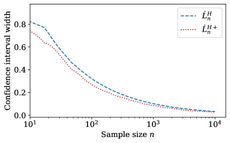
Figure 3: Two $(90\%,2)$-LPCIs: $\dot{L}_{n}^{H}$ given in (11) and $\dot{L}_{n}^{H+}$ given in (12) — i.e. these are $(1-\alpha,\varepsilon)$-LPCIs with $\alpha=0.1$ and $\varepsilon=2$. Notice that the latter can be tighter than the former. Indeed this is because $L_{n}^{H+}$ is never looser than $L_{n}^{H}$ (by definition) but strictly tighter with positive probability.

In fact, we can strictly improve on (11) by exploiting the martingale dependence of this problem. Indeed, under the same assumptions as Theorem 4, we have that

$$\small\dot{L}_{n}^{\mathrm{H}+}:=\max_{1\leq t\leq n}\left\{\widehat{\mu}_{t}-\frac{\log(1/\alpha)+t\lambda_{n}^{2}/8}{\lambda_{n}\sum_{i=1}^{t}r_{i}}\right\}$$ (12)

is also a lower $(1-\alpha,(\varepsilon_{t})_{{t}={1}}^{n})$-LPCI for $\mu^{\star}$, where $\lambda_{n}:=\sqrt{8\log(1/\alpha)/n}$. Notice that $\dot{L}_{n}^{\mathrm{H}+}$ is at least as tight as $\dot{L}_{n}^{\mathrm{H}}$ since the $n^{\mathrm{th}}$ term in the above $\max_{1\leq t\leq n}$ recovers $\dot{L}_{n}^{\mathrm{H}}$ exactly. Moreover, $\dot{L}_{n}^{\mathrm{H}+}$ is strictly tighter than $\dot{L}_{n}^{\mathrm{H}}$ with positive probability, and hence strictly tighter in expectation: $\mathbb{E}(\dot{L}_{n}^{\mathrm{H}+})>\mathbb{E}(\dot{L}_{n}^{\mathrm{H}})$.

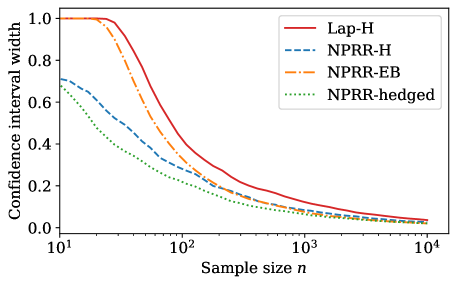
Figure 4: Widths of $(90\%,2)$-LPCIs for the mean of a Beta(50, 50) distribution. Hoeffding-based methods (Lap-H and NPRR-H found in Corollary 4 and Theorem 4) do slightly worse than the variance-adaptive ones (NPRR-EB and NPRR-hedged in Proposition 2 and Theorem 10), but in all cases, CIs that rely on NPRR seem to outperform Lap-H in both small and large $n$ regimes.

Remark 5 (Minimax rate optimality of (11)).

In the case of $\varepsilon_{1}=\dots=\varepsilon_{n}=\varepsilon\in(0,1]$, Duchi et al. [24, Proposition 1] give minimax estimation rates for the problem of nonparametric mean estimation. Their lower bounds say that for any $\varepsilon$-LDP mechanism and estimator $\widehat{\mu}_{n}$ for $\mu^{\star}$, the root mean squared error $\sqrt{\mathbb{E}(\widehat{\mu}_{n}-\mu^{\star})^{2}}$ cannot scale faster than $O(1/\sqrt{n\varepsilon^{2}})$. Since NPRR is $\varepsilon$-LDP with $\varepsilon=\log(1+2r/(1-r))$, we have that $r\asymp\varepsilon$ up to constants on $\varepsilon\in(0,1]$. It follows that $\dot{L}_{n}^{\mathrm{H}}\asymp 1/\sqrt{n\varepsilon^{2}}$, matching the minimax estimation rate. Of course, the midpoint of a CI for $\mu^{\star}$ can always be used as an estimator for $\mu^{\star}$, and hence we cannot expect the width of the CI to shrink faster than the minimax estimation rate. While explicit minimax lower bounds do not exist for the setting where $\varepsilon_{i}\neq\varepsilon_{j}$ for some $i,j$, notice that instead of scaling with $r^{-1}$ (which we would have if $r_{i}=r_{j}$ for $i\neq j$), $\dot{L}_{n}^{\mathrm{H}}$ scales with $(\frac{1}{n}\sum_{i=1}^{n}r_{i})^{-1}$, and hence our bounds seem to be of the right order when $\varepsilon$ is permitted to change.

Remark 6 (The relationship between $\varepsilon$ and (11) for practical levels of privacy).

As mentioned in the introduction and in Figure 1, Apple uses values of $\varepsilon\in\{2,4,8\}$ for various $\varepsilon$-LDP data collection tasks on iPhones [7]. Note that for $G=1$, having $\varepsilon$ take values of 2, 4, and 8 corresponds to $r$ being roughly 0.762, 0.964, and 0.999, respectively, via the relationship $r=(\exp(\varepsilon)-1)/(\exp(\varepsilon)+1)$. As such, (11) simply inflates the width of the non-private Hoeffding CI by $0.762^{-1}$, $0.964^{-1}$, and $0.999^{-1}$, respectively. Hence larger $\varepsilon$ (e.g. $\varepsilon\geq 4$) leads to CIs that are nearly indistinguishable from the non-private case (Figure 1).

Remark 7.

Since Hoeffding-type bounds are not variance-adaptive (meaning they use a worst-case upper-bound on the variance of bounded random variables as in Hoeffding [35]), they do not benefit from the additional granularity when setting $G_{t}\geq 2$ (see Section B.3 for a detailed mathematical explanation). As such, we set $G_{t}=1$ for each $t$ when running NPRR-H. Nevertheless, other CIs are capable of adapting to the variance with $G_{t}\geq 2$, and these are discussed in Section B.5, with some suggestions for how to choose $G_{t}\geq 2$ in Section B.6. Nevertheless, the empirical performance of our variance-adaptive CIs is illustrated in Fig. 4.

3.3 Time-uniform Confidence Sequences for $\mu^{\star}$

Previously, we focused on constructing a (lower) CI $L_{n}$ for $\mu^{\star}$, meaning that $L_{n}$ satisfies the high-probability guarantee $\mathbb{P}(\mu^{\star}\geq L_{n})\geq 1-\alpha$ for the prespecified sample size $n$. We will now derive CSs — i.e. entire sequences of CIs $(L_{t})_{t=1}^{\infty}$ — which have the stronger time-uniform coverage guarantee $\mathbb{P}(\forall t,\ \mu^{\star}\geq L_{t})\geq 1-\alpha$, enabling anytime-valid inference in sequential regimes. See Section 1.2 for a review of the mathematical and practical differences between CIs and CSs. In summary, if $(L_{t})_{t=1}^{\infty}$ is a lower $(1-\alpha)$-CS, then $L_{\tau}$ forms a valid $(1-\alpha)$-CI at arbitrary stopping times $\tau$ (including random and data-dependent times) and hence a practitioner can continuously update inferences as new data are collected, without any penalties for “peeking” at the data early. Let us now present a Hoeffding-type CS for $\mu^{\star}$, serving as a time-uniform analogue of Theorem 4.

Theorem 8 (NPRR-H-CS).

Let $(Z_{t})_{{t}={1}}^{\infty}\sim Q$ for some $Q\in\mathcal{Q}_{\mu^{\star}}^{\infty}$. Define the modified mean estimator under NPRR:

$$\small\widehat{\mu}_{t}(\lambda_{1}^{t}):=\frac{\sum_{i=1}^{t}\lambda_{i}\cdot(Z_{i}-(1-r_{i})/2)}{\sum_{i=1}^{t}r_{i}\lambda_{i}},$$ (13)

and let $(\lambda_{t})_{{t}={1}}^{\infty}$ be a real-valued sequence of tuning parameters (discussed in (34)). Then,

$$\small\bar{L}_{t}^{\mathrm{H}}:=\widehat{\mu}_{t}(\lambda_{1}^{t})-\frac{\log(1/\alpha)+\sum_{i=1}^{t}\lambda_{i}^{2}/8}{\sum_{i=1}^{t}r_{i}\lambda_{i}}$$ (14)

forms a lower $(1-\alpha,(\varepsilon_{t})_{t})$-LPCS for $\mu^{\star}$.

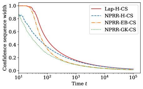
Figure 5: Widths of (90%, 2)-LPCSs for the mean of a Beta(50, 50) distribution. Like Figure 4, Hoeffding-based methods (Lap-H-CS and NPRR-H-CS found in Proposition 1 and Theorem 8) do worse than the variance-adaptive ones (NPRR-EB-CS and NPRR-GK-CS in Proposition 3 and Theorem 11) for large $t$, though NPRR-H-CS does outperform NPRR-EB-CS for small $t$. Nevertheless, in all cases, we find that NPRR-based CSs outperform Lap-H-CS in both small and large $t$ regimes.

The proof can be found in Section A.4. Unlike Theorem 4, we suggest setting

$$\small\lambda_{t}:=\sqrt{\frac{8\log(1/\alpha)}{t\log(t+1)}}\land 1,$$ (15)

to ensure that $\bar{L}_{t}^{\mathrm{H}}\asymp O(\sqrt{\log t/t})$ up to $\log\log t$ factors. Waudby-Smith and Ramdas [70, Section 3.3] give a derivation and discussion of $\lambda_{t}$ and the $O(\sqrt{\log t/t})$ rate. Similar to Theorem 4, we recommend setting $r_{t}$ for the desired $\varepsilon_{t}$-LDP level via (6) and $G_{t}:=1$ for all $t$.

The similarity between Theorem 8 and Theorem 4 is no coincidence: indeed, Theorem 4 is a corollary of Theorem 8 where we instantiated a CS at a fixed sample size $n$ and set $\lambda_{1}=\cdots=\lambda_{n}=\sqrt{8\log(1/\alpha)/n}$. In fact, every Cramér-Chernoff bound (even in the non-private regime) has an underlying supermartingale and CS that are rarely exploited [37], but setting $\lambda$’s as in Theorem 4 tightens these CSs for the fixed time $n$ — yielding $O(1/\sqrt{n})$ rates but only for a fixed $n$ — while tuning $\lambda_{t}$ as in (15) allows them to spread their efficiency over all $t$ — yielding $O(\sqrt{\log t/t})$ rates but for all $t$ simultaneously. Notice that both the time-uniform and fixed-time bounds in Theorems 4 and 8 cover an unchanging real-valued mean $\mu^{\star}\in\mathbb{R}$ — in the following section, we will relax this assumption and allow for the mean of each $X_{i}$ to change over time in an arbitrary matter, but still derive CSs for sensible parameters.

3.4 Confidence Sequences for Time-varying Means

All of the bounds derived thus far have been concerned with estimating some common $\mu^{\star}$ under the nonparametric assumption $(X_{t})_{{t}={1}}^{\infty}\sim P$ for some $P\in\mathcal{P}_{\mu^{\star}}^{\infty}$ and hence $(Z_{t})_{{t}={1}}^{\infty}\sim Q$ for some $Q\in\mathcal{Q}_{\mu^{\star}}^{\infty}$. Let us now consider the more general (and challenging) task of constructing CSs for the average mean so far $\widetilde{\mu}_{t}^{\star}:=\frac{1}{t}\sum_{i=1}^{t}\mu_{i}^{\star}$ under the assumption that each $X_{t}$ has a different mean $\mu_{t}^{\star}$. In what follows, we require that NPRR is non-interactive, i.e. $r_{t}=r\in(0,1]$ and $G_{t}=G\in\{1,2,\dots\}$ for each $t$.

Theorem 9 (Confidence sequences for time-varying means).

Suppose $X_{1},X_{2},\dots$ are independent $[0,1]$-bounded random variables with individual means $\mathbb{E}X_{t}=\mu_{t}^{\star}$ for each $t$, and let $Z_{1},Z_{2}\dots$ be their privatized views according to NPRR without sequential interactivity. Define

$$\widehat{\mu}_{t} :=\frac{\sum_{i=1}^{t}(Z_{i}-(1-r)/2)}{tr},$$ (16)

$$\text{and}~{}~{}\widetilde{B}_{t}^{\pm} :=\sqrt{\frac{t\beta^{2}+1}{2(tr\beta)^{2}}\log\left(\frac{\sqrt{t\beta^{2}+1}}{\alpha}\right)},$$ (17)

for any $\beta>0$. Then, $\widetilde{C}_{t}^{\pm}:=(\widehat{\mu}_{t}\pm\widetilde{B}_{t}^{\pm})$ forms a two-sided $(1-\alpha,\varepsilon)$-LPCS for $\widetilde{\mu}_{t}^{\star}$, where $\varepsilon=\log(1+\frac{2r}{1-r})$.

The proof in Section A.5 uses a sub-Gaussian mixture supermartingale technique similar to Robbins [54] and Howard et al. [37, 38]. The parameter $\beta>0$ is a tuning parameter dictating a time for which the CS boundary is optimized. Regardless of how $\beta$ is chosen, $\widetilde{C}_{t}^{\pm}$ has the time-uniform coverage guarantee given in Theorem 9 but finite-sample performance can be improved near a particular time $t_{0}$ by selecting

$$\small\beta_{\alpha}(t_{0}):=\sqrt{\frac{-2\log\alpha+\log(-2\log\alpha+1)}{t_{0}}},$$ (18)

which approximately minimizes $\widetilde{B}_{t_{0}}$; see Howard et al. [38, Section 3.5] for details.

Notice that in the non-private case where $r=1$, we have that $\widetilde{C}_{t}^{\pm}$ recovers Robbins’ sub-Gaussian mixture CS [54, 38]. Notice that while Theorem 9 handles a strictly more general and challenging problem than the previous sections (by tracking a time-varying mean $(\widetilde{\mu}_{t})_{t=1}^{\infty}$), it has the restriction that NPRR must be non-interactive. There is a technical reason for this that boils down to it being difficult to combine time-varying tuning parameters (such as those in Theorem 8) with time-varying estimands in the same CS. This challenge has appeared in other (non-private) works on CSs [70, 38]. In short, this paper has methods for tracking a time-varying mean under non-interactive NPRR or a fixed mean under sequentially interactive NPRR, but not both simultaneously — this would be an interesting direction to explore in future work.

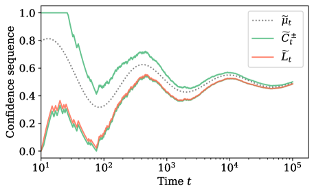
Figure 6: $(90\%,2)$-LPCSs for the average time-varying mean so far $\widetilde{\mu}_{t}^{\star}$ with the boundary optimized for $t_{0}=100$. In this example, we set $\mu_{t}^{\star}=\frac{1}{2}\left[1-\sin(2\log(e+t))/\log(e+0.01t)\right]$ to produce the displayed sinusoidal behavior. Notice that $\widetilde{L}_{t}$ is tighter at the expense of only being one-sided. In either case, however, the CSs adapt to non-stationarity and capture $\widetilde{\mu}_{t}^{\star}$ uniformly over time.

A one-sided analogue of Theorem 9 is presented in Section B.7 via slightly different techniques.

4 Illustration: Private Online A/B Testing

Our methods can be used to conduct locally private online A/B tests (sequential randomized experiments). Broadly, an A/B test is a statistically principled way of comparing two different treatments — e.g. administering drug A versus drug B in a clinical trial. In its simplest form, A/B testing proceeds by (i) randomly assigning subjects to receive treatment A with some probability $\pi\in(0,1)$ and treatment B with probability $1-\pi$, (ii) collecting some outcome measurement $Y_{t}$ for each subject $t\in\{1,2,\dots\}$ — e.g. severity of headache after taking drug A or B — and (iii) measuring the difference in that outcome between the two groups. An online A/B test is one that is conducted sequentially over time — e.g. a sequential clinical trial where patients are recruited one after the other or in batches.

We now illustrate how to sequentially test for the mean difference in outcomes between groups A and B when only given access to locally private data. To set the stage, suppose that $(A_{1},Y_{1}),(A_{2},Y_{2}),\dots$ are random variables such that $A_{t}\sim\mathrm{Bernoulli}(\pi)$ is 1 if subject $t$ received treatment A and 0 if they received treatment B, and $Y_{t}$ is a $[0,1]$-bounded outcome of interest after being assigned treatment $A_{t}$.

Using the techniques of Section 3.4, we will construct $(1-\alpha)$-CSs for the time-varying mean $\widetilde{\Delta}_{t}:=\frac{1}{t}\sum_{i=1}^{t}\Delta_{i}$ where $\Delta_{i}:={\mathbb{E}(Y_{i}\mid A_{i}=1)}-{\mathbb{E}(Y_{i}\mid A_{i}=0)}$ is the mean difference in the outcomes at time $i$. In words, $\widetilde{\Delta}_{t}$ is the mean difference in outcomes among the subjects so far.

Unlike Section 3.4, however, we will not directly privatize $(Y_{t})_{{t}={1}}^{\infty}$, but instead will apply NPRR to some “pseudo-outcomes” $\varphi_{t}\equiv\varphi_{t}(Y_{t},A_{t})$ — functions of $Y_{t}$ and $A_{t}$,

$$\varphi_{t}:=\frac{f_{t}+\frac{1}{1-\pi}}{\frac{1}{\pi}+\frac{1}{1-\pi}},~{}~{}\text{where}~{}~{}f_{t}:=\left[\frac{Y_{t}A_{t}}{\pi}-\frac{Y_{t}(1-A_{t})}{1-\pi}\right].$$

Notice that due to the fact that $Y_{t},A_{t}\in[0,1]$, we have $f_{t}\in[-1/(1-\pi),1/\pi]$, and hence $\varphi_{t}\in[0,1]$. Now that we have $[0,1]$-bounded random variables $(\varphi_{t})_{{t}={1}}^{\infty}$, we can obtain their NPRR-induced $\varepsilon$-LDP views $(\psi_{t})_{{t}={1}}^{\infty}$ by setting $G_{t}=1$ and $r_{t}=\exp\{\varepsilon-1\}/\exp\{\varepsilon+1\}$ for each $t$. Notice that we are privatizing $\varphi_{t}$ which is a function of both $Y_{t}$ and $A_{t}$, so both the outcome and the treatment are protected with $\varepsilon$-LDP.

Corollary 1 (Locally private online A/B estimation).

Following the setup above, let $(\psi_{t})_{{t}={1}}^{\infty}$ be the NPRR-induced privatized views of $(\varphi_{t})_{{t}={1}}^{\infty}$. Define the estimator

$$\widehat{\varphi}_{t} :=\frac{\sum_{i=1}^{t}(\psi_{i}-(1-r)/2)}{tr},$$ (19)

and set $\widetilde{B}_{t}$ as in (46). Then,

$$\small\widetilde{L}_{t}^{\Delta}:=-\frac{1}{1-\pi}+\left(\frac{1}{\pi}+\frac{1}{1-\pi}\right)\left(\widehat{\varphi}_{t}-\widetilde{B}_{t}\right)$$ (20)

is a lower $(1-\alpha,\varepsilon)$-LPCS for $\widetilde{\Delta}_{t}$.

The proof is an immediate consequence of the well-known fact about “inverse-probability-weighted” estimators that $\mathbb{E}f_{t}=\Delta_{t}$ for every $t$ [36, 55], combined with Proposition 4. Similarly, a two-sided CS can be obtained by replacing $\widehat{\varphi}_{t}-\widetilde{B}_{t}$ in (20) with $\widehat{\varphi}_{t}\pm\widetilde{B}_{t}^{\pm}$, where $\widetilde{B}_{t}^{\pm}$ is given in (17).

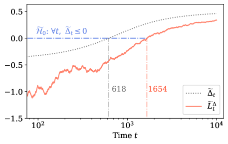
Figure 7: An example of Corollary 1 applied to the time-varying mean given by $\Delta_{t}:=1.8(\exp\{t/300\}/(1+\exp\{t/300\})-1/2)$. In this particular example, we have that $\widetilde{\Delta}_{t}:=\frac{1}{t}\sum_{i=1}^{t}\Delta_{i}$ changes from negative to positive at time 618, and yet our lower CS $\widetilde{L}_{t}^{\Delta}$ later detects this change at time 1654, at which point the weak null $\widetilde{\mathcal{H}}_{0}$: $\forall t,\ \widetilde{\Delta}_{t}\leq 0$ can be rejected (see Section B.9 for details regarding the composite hypothesis $\widetilde{\mathcal{H}}_{0}$ and how to test it).

Practical implications. The implications of Corollary 1 for the practitioner are threefold:

1. The CSs can be continuously monitored from the start of the A/B test and for an indefinite amount of time;

2. Inferences made from $\widetilde{L}_{\tau}^{\Delta}$ are valid at any stopping time $\tau$, regardless of why the test is stopped; and

3. $\widetilde{L}_{t}^{\Delta}$ adapts to non-stationarity: if the treatment differences $\Delta_{t}$ drift over time, $\widetilde{L}_{t}^{\Delta}$ still forms an LPCS for $\widetilde{\Delta}_{t}$. But if $\Delta_{1}=\Delta_{2}=\dots=\Delta^{\star}$ is constant, then $\widetilde{L}_{t}^{\Delta}$ forms an LPCS for $\Delta^{\star}$.

5 Additional Results & Summary

Both NPRR and our proof techniques are general-purpose tools with several other implications for locally private statistical inference, including confidence sets via the Laplace mechanism, variance-adaptive inference, and sequential hypothesis testing. We briefly expand on these implications here, and leave their details to the appendix.

• §B.4: Confidence sets via the Laplace mechanism. We introduced NPRR as an extension of randomized response for arbitrary bounded data (rather than just binary), but of course the Laplace mechanism also handles bounded data. While NPRR enjoys advantages over Laplace as discussed in Section 2, it may still be of interest to derive confidence sets from data that are privatized via Laplace, given its ubiquity and simplicity. Section B.4 presents new nonparametric CIs and CSs for population means under the Laplace mechanism.

• §B.5: Variance-adaptive inference. Notice that the CIs and CSs presented in Section 3 were not variance-adaptive due to the fact that they relied on sub-Gaussianity of bounded random variables. However, this is not necessary, and we present other locally private variance-adaptive CIs and CSs in Section B.5.

• §B.8: Sequential hypothesis testing. While the statistical procedures of this paper have taken the form of CIs and CSs rather than hypothesis tests, there is a deep relationship between the two, and our results have analogues that could have been presented in the language of the latter. Section B.8 articulates this relationship and presents explicit (sequential) tests.

• §B.10: Adaptive online A/B testing. Corollary 1 assumes a common propensity score $\pi$ among all subjects for simplicity of exposition, but it is also possible to derive CSs for $\widetilde{\Delta}_{t}$ under an adaptive framework where propensity scores $(\pi_{t}(X_{t}))_{t=1}^{\infty}$ can change over time in a data-dependent fashion, and be functions of some measured covariates $(X_{t})_{t=1}^{\infty}$. The details of this more complex setup are left to Section B.10.

Another followup problem that we do not explicitly address here but that can be solved using our techniques is locally private variance estimation. Notice that the variance $\mathrm{Var}(X):=\mathbb{E}(X^{2})-(\mathbb{E}(X))^{2}$ is a function of two expectations, $\mathbb{E}(X^{2})$ and $\mathbb{E}(X)$. Since $X^{2}$ is also $[0,1]$-bounded if $X$ is, we can use all of the techniques in this paper to derive two separate $(1-\alpha/2,\varepsilon/2)$-LPCIs (or LPCSs) to derive a $(1-\alpha,\varepsilon)$-LPCI for $\mathrm{Var}(X)$. Of course this requires collecting privatized views of both $X^{2}$ and $X$ separately. As a further generalization, a similar argument can be made for the construction of LPCIs for the covariance of $X$ and $Y$ since $\mathrm{Cov}(X,Y)=\mathbb{E}(XY)-\mathbb{E}(X)\mathbb{E}(Y)$ (though here we would need to construct $(1-\alpha/3,\varepsilon/3)$-LPCIs, etc.).

A limitation of the present paper is that we have only discussed confidence sets for univariate parameters. Indeed, it is not immediately clear to us what is the right way to generalize NPRR to the multivariate case, or how to derive LPCIs and LPCSs for means of random vectors given such a generalization. This is an open direction for future work.

With the growing interest in protecting user privacy, an increasingly important addition to the statistician’s toolbox are methods that can extract population information from privatized data. In this paper, we derived nonparametric confidence intervals and time-uniform confidence sequences for population means from locally private data. We introduced, NPRR a nonparametric and sequentially interactive extension of Warner’s randomized response for bounded data. The privatized output from NPRR can then be harnessed to produce confidence sets for the mean of the raw data distribution. Importantly, our confidence sets are sharp, some attaining optimal theoretical convergence rates and others simply having excellent empirical performance, not only making private nonparametric (sequential) inference possible, but practical. In future work, we aim to apply these general-purpose tools to changepoint detection, two-sample testing, and (conditional) independence testing.

Acknowledgments.

ZSW was supported in part by NSF CNS2120667. AR acknowledges NSF DMS2310718.

Appendix A Proofs of main results

A.1 Prelude: filtrations, supermartingales, and Ville’s inequality

By far the most common way to derive a CS is by constructing a nonnegative supermartingales and then applying Ville’s maximal inequality to it. Indeed, all of the proofs for our CS and CI results employ this technique. However, in order to discuss supermartingales we must first review filtrations. A filtration $\mathcal{F}\equiv(\mathcal{F}_{t})_{{t}={0}}^{\infty}$ is a nondecreasing sequence of sigma-algebras $\mathcal{F}_{0}\subseteq\mathcal{F}_{1}\subseteq\cdots$, and a stochastic process $(M_{t})_{{t}={0}}^{\infty}$ is said to be adapted to $\mathcal{F}$ if $M_{t}$ is $\mathcal{F}_{t}$-measurable for all $t\in\mathbb{N}$. On the other hand, $(M_{t})_{{t}={1}}^{\infty}$ is said to be $\mathcal{F}$-predictable if each $M_{t}$ is $\mathcal{F}_{t-1}$-measurable — informally “$M_{t}$ depends on the past”.

For example, the canonical filtration $\mathcal{X}$ generated by a sequence of random variables $(X_{t})_{{t}={1}}^{\infty}$ is given by the sigma-algebra generated by $X_{1}^{t}$, i.e. $\mathcal{X}_{t}:=\sigma(X_{1}^{t})$ for each $t\in\{1,2,\dots\}$, and $\mathcal{X}_{0}$ is the trivial sigma-algebra. A function $M_{t}\equiv M(X_{1}^{t})$ depending only on $X_{1}^{t}$ forms a $\mathcal{X}$-adapted process, while $(M_{t-1})_{t=1}^{\infty}$ is $\mathcal{X}$-predictable. Likewise, if we obtain a privatized view $(Z_{t})_{{t}={1}}^{\infty}$ of $(X_{t})_{{t}={1}}^{\infty}$ using some locally private mechanism, a different filtration $\mathcal{Z}$ emerges, given by $\mathcal{Z}_{t}:=\sigma(Z_{1}^{t})$. Throughout our proofs, $\mathcal{Z}$-adapted and $\mathcal{Z}$-predictable processes will be central mathematical objects.

A process $(M_{t})_{{t}={0}}^{\infty}$ adapted to $\mathcal{F}$ is a supermartingale if

$$\small\mathbb{E}(M_{t}\mid\mathcal{F}_{t-1})\leq M_{t-1}~{}~{}\text{for each $t\geq 1$.}$$ (21)

If the above inequality is replaced by an equality, then $(M_{t})_{{t}={0}}^{\infty}$ is a martingale. The methods in this paper will involve derivations of (super)martingales which are nonnegative and begin at one — often referred to as “test (super)martingales” [57] or simply “nonnegative (super)martingales” (NMs or NSMs for martingales and supermartingales, respectively) [54, 37]. NSMs $(M_{t})_{{t}={0}}^{\infty}$ satisfy the following powerful concentration inequality due to Ville [59]:

$$\small\mathbb{P}(\exists t\in\mathbb{N}:M_{t}\geq 1/\alpha)\leq\alpha.$$ (22)

In other words, they are unlikely to ever grow too large.

In the CS proofs that follow, we will focus on deriving processes $(M_{t}(\mu))_{t=1}^{\infty}$ for any $\mu\in[0,1]$ such that when $\mu$ is equal to the true mean of interest $\mu^{\star}$, we have that $M_{t}(\mu^{\star})$ forms a NSM. In this case, it turns out that the set of $\mu$ such that $M_{t}(\mu)$ is less than $1/\alpha$ — i.e. $C_{t}:=\{\mu\in[0,1]:M_{t}(\mu)<1/\alpha\}$ — forms a $(1-\alpha)$-CS for $\mu^{\star}$. This is easy to see since $\mu^{\star}\notin C_{t}$ if and only if $M_{t}(\mu^{\star})\geq 1/\alpha$, and thus

$$\mathbb{P}(\exists t\in\mathbb{N}:\mu^{\star}\notin C_{t})=\mathbb{P}(\exists t\in\mathbb{N}:M_{t}(\mu^{\star})\geq 1/\alpha)\leq\alpha,$$ (23)

where the last inequality is precisely (22). The CS proofs that follow will make the exact processes $(M_{t}(\mu))_{t=1}^{\infty}$ explicit.

A.2 Proof of Theorem 1

See 1

Proof.

We will prove the result for fixed $r\in(0,1),G\geq 1$ but it is straightforward to generalize the proof for $r_{t}$ depending on $Z_{1}^{t-1}$. It suffices to verify that the likelihood ratio $L(x,\widetilde{x})$ is bounded above by $\exp(\varepsilon)$ for any $x,\widetilde{x}\in[0,1]$. Writing out the likelihood ratio $L(x,\widetilde{x})$, we have

$$L(x,\widetilde{x}):=\frac{\frac{1-r}{G+1}+rG\cdot\left\{\mathds{1}(Z=x^{\mathrm{ceil}})(x-x^{\mathrm{floor}})+\mathds{1}(Z=x^{\mathrm{floor}})\left[1/G-(x-x^{\mathrm{floor}})\right]\right\}}{\frac{1-r}{G+1}+rG\cdot\left\{\mathds{1}(Z=\widetilde{x}^{\mathrm{ceil}})(\widetilde{x}-\widetilde{x}^{\mathrm{floor}})+\mathds{1}(Z=\widetilde{x}^{\mathrm{floor}})\left[1/G-(\widetilde{x}-\widetilde{x}^{\mathrm{floor}})\right]\right\}},$$

which is dominated by the counting measure. Notice that the numerator of $L$ is maximized when $x$ already lies in the discretized range, i.e. $Z=x=x^{\mathrm{ceil}}=x^{\mathrm{floor}}$ so that the numerator becomes $\frac{1-r}{G+1}+r$, while the denominator is minimized when $Z\neq\widetilde{x}^{\mathrm{ceil}}$ and $Z\neq\widetilde{x}^{\mathrm{floor}}$ so that the denominator becomes $\frac{1-r}{G+1}$. Therefore, we have that with probability one,

$$L(x,\widetilde{x})\leq\frac{\frac{1-r}{G+1}+r}{\frac{1-r}{G+1}}=1+\frac{(G+1)r}{1-r},$$

and thus NPRR is $\varepsilon$-locally DP with $\varepsilon:=\log(1+(G+1)r/(1-r))$. ∎

A.3 Proof of Theorem 4

See 4

Proof.

The proof proceeds in two steps. First we note that $\bar{L}_{t}^{\mathrm{H}}$ forms a $(1-\alpha)$-lower confidence sequence, and then instantiate this fact at the sample size $n$.

Step 1. $\bar{L}_{t}^{\mathrm{H}}$ forms a $(1-\alpha)$-lower CS.

This is exactly the statement of Theorem 8.

Step 2. $\dot{L}_{n}^{\mathrm{H}}$ is a lower-CI.

By Step 1, we have that $\bar{L}_{t}^{\mathrm{H}}$ forms a $(1-\alpha)$-lower CS, meaning

$$\mathbb{P}(\forall t\in\{1,\dots,n\},\ \mu^{\star}\geq\bar{L}_{t}^{\mathrm{H}})\geq 1-\alpha.$$

Therefore,

$$\mathbb{P}\left(\mu^{\star}\geq\max_{1\leq t\leq n}\bar{L}_{t}^{\mathrm{H}}\right)=\mathbb{P}(\mu^{\star}\geq\dot{L}_{n}^{\mathrm{H}})\geq 1-\alpha,$$

which completes the proof. ∎

A.4 Proof of Theorem 8

See 8

Proof.

The proof proceeds in two steps. First, we construct an NSM adapted to the private filtration $\mathcal{Z}\equiv(\mathcal{Z}_{t})_{{t}={0}}^{\infty}$. Second and finally, we apply Ville’s inequality to obtain a high-probability upper bound on the NSM, and show that this inequality results in the CS given in Theorem 8.

Step 1.

Consider the nonnegative process starting at one given by

$$M_{t}(\mu^{\star}):=\prod_{i=1}^{t}\exp\left\{\lambda_{i}(Z_{i}-\zeta_{i}(\mu^{\star}))-\lambda_{i}^{2}/8\right\},$$ (24)

where $(\lambda_{t})_{{t}={1}}^{\infty}$ is a real-valued sequence and $\zeta_{t}(\mu^{\star}):=r_{t}\mu^{\star}+(1-r_{t})/2$ as usual. We claim that $(M_{t}(\mu^{\star}))_{t=0}^{\infty}$ is a supermartingale, meaning $\mathbb{E}(M_{t}(\mu^{\star})\mid\mathcal{Z}_{t-1})\leq M_{t-1}(\mu^{\star})$. Writing out the conditional expectation of $M_{t}(\mu^{\star})$, we have

$$\mathbb{E}\left(M_{t}(\mu^{\star})\mid\mathcal{Z}_{t-1}\right)$$

$$=\ \mathbb{E}\left(\prod_{i=1}^{t}\exp\left\{\lambda_{i}(Z_{i}-\zeta_{i}(\mu^{\star}))-\lambda_{i}^{2}/8\right\}\biggm{|}\mathcal{Z}_{t-1}\right)$$

$$=\ \underbrace{\prod_{i=1}^{t-1}\exp\left\{\lambda_{i}(Z_{i}-\zeta_{i}(\mu^{\star}))-\lambda_{i}^{2}/8\right\}}_{M_{t-1}(\mu^{\star})}\cdot\underbrace{\mathbb{E}\left(\exp\left\{\lambda_{t}(Z_{t}-\zeta_{t}(\mu^{\star}))-\lambda_{t}^{2}/8\right\}\biggm{|}\mathcal{Z}_{t-1}\right)}_{(\dagger)},$$

since $M_{t-1}(\mu^{\star})$ is $\mathcal{Z}_{t-1}$-measurable, and thus it can be written outside of the conditional expectation. It now suffices to show that $(\dagger)\leq 1$. To this end, note that $Z_{t}$ is a $[0,1]$-bounded random variable with conditional mean $\mathbb{E}(Z_{t}\mid\mathcal{Z}_{t-1})=\zeta_{t}(\mu^{\star})$ by design of NPRR (Algorithm 2). Since bounded random variables are sub-Gaussian [35], we have that

$$\mathbb{E}(\lambda_{t}(Z_{t}-\zeta_{t}(\mu^{\star}))\mid\mathcal{Z}_{t-1})\leq\exp\left\{\lambda_{t}^{2}/8\right\},$$

and hence $(\dagger)\leq 1$. Therefore, $(M_{t}(\mu^{\star}))_{t=0}^{\infty}$ is a $\mathcal{Q}_{\mu^{\star}}^{\infty}$-NSM.

Step 2.

By Ville’s inequality for NSMs [59], we have that

$$\mathbb{P}(\exists t:M_{t}(\mu^{\star})\geq 1/\alpha)\leq\alpha.$$

In other words, we have that $M_{t}(\mu^{\star})<1/\alpha$ for all $t\in\mathbb{N}$ with probability at least $1-\alpha$. Using some algebra to rewrite the inequality $M_{t}(\mu^{\star})<1/\alpha$, we have

$$M_{t}(\mu^{\star})<1/\alpha \iff\prod_{i=1}^{t}\exp\left\{\lambda_{i}(Z_{i}-\zeta_{i}(\mu^{\star}))-\lambda_{i}^{2}/8\right\}<\frac{1}{\alpha}$$

$$\iff\sum_{i=1}^{t}\left[\lambda_{i}(Z_{i}-\zeta_{i}(\mu^{\star}))-\lambda_{i}^{2}/8\right]<\log(1/\alpha)$$

$$\iff\sum_{i=1}^{t}\lambda_{i}Z_{i}-\mu^{\star}\sum_{i=1}^{t}\lambda_{i}r_{i}-\sum_{i=1}^{t}\lambda_{i}\cdot(1-r_{i})/2-\sum_{i=1}^{t}\lambda_{i}^{2}/8<\log(1/\alpha)$$

$$\iff\mu^{\star}>\underbrace{\frac{\sum_{i=1}^{t}\lambda_{i}\cdot(Z_{i}-(1-r_{i})/2)}{\sum_{i=1}^{t}r_{i}\lambda_{i}}}_{\widehat{\mu}_{t}(\lambda_{1}^{t})}-\underbrace{\frac{\log(1/\alpha)+\sum_{i=1}^{t}\lambda_{i}^{2}/8}{\sum_{i=1}^{t}r_{i}\lambda_{i}}}_{\bar{B}_{t}(\lambda_{1}^{t})}$$

Therefore, $\bar{L}_{t}:=\widehat{\mu}_{t}(\lambda_{1}^{t})-\bar{B}_{t}(\lambda_{1}^{t})$ forms a lower $(1-\alpha)$-CS for $\mu^{\star}$. The upper CS $\bar{U}_{t}:=\widehat{\mu}_{t}(\lambda_{1}^{t})+\bar{B}_{t}(\lambda_{1}^{t})$ can be derived by applying the above proof to $(-Z_{t})_{{t}={1}}^{\infty}$ and their conditional means $(-\zeta_{i}(\mu^{\star}))_{t=1}^{\infty}$. This completes the proof

∎

A.5 Proof of Theorem 9

See 9

Proof.

The proof proceeds in three steps. First, we derive a sub-Gaussian NSM indexed by a parameter $\lambda\in\mathbb{R}$. Second, we mix this NSM over $\lambda$ using the density of a Gaussian distribution, and justify why the resulting process is also an NSM. Third and finally, we apply Ville’s inequality and invert the NSM to obtain $(\widetilde{C}^{\pm}_{t})_{{t}={1}}^{\infty}$.

Step 1: Constructing the $\lambda$-indexed NSM.

Let $(X_{t})_{{t}={1}}^{\infty}$ be independent $[0,1]$-bounded random variables with individual means given by $\mathbb{E}X_{t}=\mu_{t}^{\star}$, and let $(Z_{t})_{{t}={1}}^{\infty}$ be the NPRR-induced private views of $(X_{t})_{{t}={1}}^{\infty}$. Define $\zeta(\mu):=r\mu+(1-r)/2$ for any $\mu\in[0,1]$, and $r\in(0,1]$. Let $\lambda\in\mathbb{R}$ and consider the process,

$$M_{t}(\lambda):=\prod_{i=1}^{t}\exp\left\{\lambda(Z_{i}-\zeta(\mu_{i}^{\star}))-\lambda^{2}/8\right\},$$ (25)

with $M_{0}(\lambda)\equiv 0$. We claim that (25) forms an NSM with respect to the private filtration $\mathcal{Z}$. The proof technique is nearly identical to that of Theorem 8 but with changing means and $\lambda=\lambda_{1}=\lambda_{2}=\cdots\in\mathbb{R}$. Indeed, $M_{t}(\lambda)$ is nonnegative with initial value one by construction, so it remains to show that $(M_{t}(\lambda))_{t=0}^{\infty}$ is a supermartingale. That is, we need to show that for every $t$, we have $\mathbb{E}(M_{t}(\lambda)\mid\mathcal{Z}_{t-1})\leq M_{t-1}(\lambda)$. Writing out the conditional expectation of $M_{t}(\lambda)$, we have

$$\mathbb{E}(M_{t}(\lambda)\mid\mathcal{Z}_{t-1}) =\mathbb{E}\left(\prod_{i=1}^{t}\exp\left\{\lambda(Z_{i}-\zeta(\mu_{i}^{\star}))-\lambda^{2}/8\right\}\Bigm{|}Z_{1}^{t-1}\right)$$

$$=\underbrace{\prod_{i=1}^{t-1}\exp\left\{\lambda(Z_{i}-\zeta(\mu_{i}^{\star}))-\lambda^{2}/8\right\}}_{M_{t-1}(\lambda)}\cdot\mathbb{E}\left(\exp\left\{\lambda(Z_{t}-\zeta(\mu_{t}^{\star}))-\lambda^{2}/8\right\}\mid Z_{1}^{t-1}\right)$$

$$=M_{t-1}(\lambda)\cdot\underbrace{\mathbb{E}\left(\exp\left\{\lambda(Z_{t}-\zeta(\mu_{t}^{\star}))-\lambda^{2}/8\right\}\right)}_{(\dagger)},$$

where the last inequality follows by independence of $(Z_{t})_{{t}={1}}^{\infty}$, and hence the conditional expectation becomes a marginal expectation. Therefore, it now suffices to show that $(\dagger)\leq 1$. Indeed, $Z_{t}$ is a $[0,1]$-bounded, mean-$\zeta(\mu_{t}^{\star})$ random variable. By Hoeffding’s sub-Gaussian inequality for bounded random variables [35], we have that ${\mathbb{E}[\exp\{\lambda(Z_{t}-\zeta(\mu_{t}^{\star}))\}]\leq\exp\{\lambda^{2}/8\}}$, and thus

$$(\dagger)=\mathbb{E}\left[\exp\left\{\lambda(Z_{t}-\zeta(\mu_{t}^{\star}))\right\}\right]\cdot\exp\left\{-\lambda^{2}/8\right\}\leq 1.$$

It follows that $(M_{t}(\lambda))_{t=0}^{\infty}$ is an NSM.

Step 2.

Let us now construct a sub-Gaussian mixture NSM. Note that the mixture of an NSM with respect to a probability distribution is itself an NSM [54, 37] — a straightforward consequence of Fubini’s theorem. Concretely, let $f_{\rho^{2}}(\lambda)$ be the probability density function of a mean-zero Gaussian random variable with variance $\rho^{2}$,

$$f_{\rho^{2}}(\lambda):=\frac{1}{\sqrt{2\pi\rho^{2}}}\exp\left\{\frac{-\lambda^{2}}{2\rho^{2}}\right\}.$$

Then, since mixtures of NSMs are themselves NSMs, the process $(M_{t})_{{t}={0}}^{\infty}$ given by

$$M_{t}:=\int_{\lambda\in\mathbb{R}}M_{t}(\lambda)f_{\rho^{2}}(\lambda)d\lambda$$ (26)

is an NSM. We will now find a closed-form expression for $M_{t}$. To ease notation, define the partial sum ${S^{\star}_{t}:=\sum_{i=1}^{t}(Z_{i}-\zeta(\mu_{i}^{\star}))}$. Writing out the definition of $M_{t}$, we have

$$M_{t} :=\int_{\lambda\in\mathbb{R}}\prod_{i=1}^{t}\exp\left\{\lambda(Z_{i}-\zeta(\mu_{i}^{\star}))-\lambda^{2}/8\right\}f_{\rho^{2}}(\lambda)d\lambda$$

$$=\int_{\lambda}\exp\left\{\lambda\underbrace{\sum_{i=1}^{t}(Z_{i}-\zeta(\mu_{i}^{\star}))}_{S^{\star}_{t}}-t\lambda^{2}/8\right\}f_{\rho^{2}}(\lambda)d\lambda$$

$$=\int_{\lambda}\exp\left\{\lambda S^{\star}_{t}-t\lambda^{2}/8\right\}\frac{1}{\sqrt{2\pi\rho^{2}}}\exp\left\{\frac{-\lambda^{2}}{2\rho^{2}}\right\}d\lambda$$

$$=\frac{1}{\sqrt{2\pi\rho^{2}}}\int_{\lambda}\exp\left\{\lambda S^{\star}_{t}-t\lambda^{2}/8\right\}\exp\left\{\frac{-\lambda^{2}}{2\rho^{2}}\right\}d\lambda$$

$$=\frac{1}{\sqrt{2\pi\rho^{2}}}\int_{\lambda}\exp\left\{\lambda S^{\star}_{t}-\frac{\lambda^{2}(t\rho^{2}/4+1)}{2\rho^{2}}\right\}d\lambda$$

$$=\frac{1}{\sqrt{2\pi\rho^{2}}}\int_{\lambda}\exp\left\{\frac{-\lambda^{2}(t\rho^{2}/4+1)+2\lambda\rho^{2}S^{\star}_{t}}{2\rho^{2}}\right\}d\lambda$$

$$=\frac{1}{\sqrt{2\pi\rho^{2}}}\int_{\lambda}\exp\left\{\frac{-a(\lambda^{2}-\frac{b}{a}2\lambda)}{2\rho^{2}}\right\}d\lambda,$$

where we have set $a:=t\rho^{2}/4+1$ and $b:=\rho^{2}S^{\star}_{t}$. Completing the square in the exponent, we have that

$$\exp\left\{\frac{-\lambda^{2}-2\lambda\frac{b}{a}+\left(\frac{b}{a}\right)^{2}-\left(\frac{b}{a}\right)^{2}}{2\rho^{2}/a}\right\} =\exp\left\{\frac{-(\lambda-b/a)^{2}}{2\rho^{2}/a}+\frac{a\left(b/a\right)^{2}}{2\rho^{2}}\right\}$$

$$=\underbrace{\exp\left\{\frac{-(\lambda-b/a)^{2}}{2\rho^{2}/a}\right\}}_{(\star)}\exp\left\{\frac{b^{2}}{2a\rho^{2}}\right\}.$$

Now notice that $(\star)$ is proportional to the density of a Gaussian random variable with mean $b/a$ and variance $\rho^{2}/a$. Plugging the above back into the integral and multiplying the entire quantity by $a^{-1/2}/a^{-1/2}$, we obtain the closed-form expression of the mixture NSM,

$$M_{t} :=\underbrace{\frac{1}{\sqrt{2\pi\rho^{2}/a}}\int_{\lambda\in\mathbb{R}}\exp\left\{\frac{-(\lambda-b/a)^{2}}{2\rho^{2}/a}\right\}d\lambda}_{=1}\frac{\exp\left\{\frac{b^{2}}{2a\rho^{2}}\right\}}{\sqrt{a}}$$

$$=\frac{1}{\sqrt{t\rho^{2}/4+1}}\exp\left\{\frac{\rho^{2}(S_{t}^{\star})^{2}}{2(t\rho^{2}/4+1)}\right\}.$$ (27)

Step 3.

Now that we have computed the mixture NSM $(M_{t})_{{t}={0}}^{\infty}$, we are ready to apply Ville’s inequality and invert the process. Since $(M_{t})_{{t}={0}}^{\infty}$ is an NSM, we have by Ville’s inequality [59],

$$\mathbb{P}(\exists t:M_{t}\geq 1/\alpha)\leq\alpha~{}~{}~{}\text{or equivalently,}~{}~{}~{}\mathbb{P}(\forall t,\ M_{t}<1/\alpha)\geq 1-\alpha.$$

Therefore, with probability at least $(1-\alpha)$, we have that for all $t\in\{1,2,\dots\}$,

$$M_{t}<1/\alpha \iff\frac{1}{\sqrt{t\rho^{2}/4+1}}\exp\left\{\frac{\rho^{2}(S_{t}^{\star})^{2}}{2(t\rho^{2}/4+1)}\right\}<1/\alpha$$

$$\iff\frac{\rho^{2}(S_{t}^{\star})^{2}}{2(t\rho^{2}/4+1)}-\log\left(\sqrt{t\rho^{2}/4+1}\right)<\log(1/\alpha)$$

$$\iff\frac{\rho^{2}(S_{t}^{\star})^{2}}{2(t\rho^{2}/4+1)}<\log\left(\frac{\sqrt{t\rho^{2}/4+1}}{\alpha}\right)$$

$$\iff(S_{t}^{\star})^{2}<\frac{2(t\rho^{2}/4+1)}{\rho^{2}}\log\left(\frac{\sqrt{t\rho^{2}/4+1}}{\alpha}\right)$$

$$\iff\frac{(S_{t}^{\star})^{2}}{t^{2}r^{2}}<\underbrace{\frac{2(t(\rho/2)^{2}+1)}{(tr\rho)^{2}}\log\left(\frac{\sqrt{t(\rho/2)^{2}+1}}{\alpha}\right)}_{(\star\star)}.$$

Set $\beta:=\rho/2$ and notice that $(\star\star)=(\widetilde{B}_{t}^{\pm})^{2}$ where $\widetilde{B}_{t}^{\pm}$ is the boundary given by (17) in the statement of Theorem 9. Also recall from Theorem 9 the private estimator $\widehat{\mu}_{t}:=\frac{1}{tr}\sum_{i=1}^{t}[Z_{i}-(1-r)/2]$ and the quantity we wish to capture — the moving average of population means $\widetilde{\mu}_{t}^{\star}:=\frac{1}{t}\sum_{i=1}^{t}\mu_{i}^{\star}$, where $\mu_{i}^{\star}=\mathbb{E}X_{i}$. Putting these together with the above high-probability bound, we have that with probability $\geq(1-\alpha)$, for all $t$,

$$M_{t}<1/\alpha \iff\frac{(S_{t}^{\star})^{2}}{t^{2}r^{2}}<(\widetilde{B}_{t}^{\pm})^{2}$$

$$\iff-\widetilde{B}_{t}^{\pm}<\frac{S^{\star}_{t}}{tr}<\widetilde{B}_{t}^{\pm}.$$

$$\iff-\widetilde{B}_{t}^{\pm}<\frac{\sum_{i=1}^{t}[Z_{i}-\zeta(\mu_{i}^{\star})]}{tr}<\widetilde{B}_{t}^{\pm}.$$

$$\iff-\widetilde{B}_{t}^{\pm}<\frac{\sum_{i=1}^{t}[Z_{i}-(r\mu_{i}^{\star}+(1-r)/2)]}{tr}<\widetilde{B}_{t}^{\pm}.$$

$$\iff-\widetilde{B}_{t}^{\pm}<\frac{\sum_{i=1}^{t}[Z_{i}-(1-r)/2]}{tr}-\frac{\bcancel{r}\sum_{i=1}^{t}\mu_{i}^{\star}}{t\bcancel{r}}<\widetilde{B}_{t}^{\pm}.$$

$$\iff-\frac{\sum_{i=1}^{t}[Z_{i}-(1-r)/2]}{tr}-\widetilde{B}_{t}^{\pm}<-\frac{\sum_{i=1}^{t}\mu_{i}^{\star}}{t}<-\frac{\sum_{i=1}^{t}[Z_{i}-(1-r)/2]}{tr}+\widetilde{B}_{t}^{\pm}.$$

$$\iff-\widehat{\mu}_{t}-\widetilde{B}_{t}^{\pm}<-\widetilde{\mu}_{t}^{\star}<-\widehat{\mu}_{t}+\widetilde{B}_{t}^{\pm}.$$

$$\iff\widehat{\mu}_{t}-\widetilde{B}_{t}^{\pm}<\widetilde{\mu}_{t}^{\star}<\widehat{\mu}_{t}+\widetilde{B}_{t}^{\pm}.$$

In summary, we have that $\widetilde{C}^{\pm}_{t}:=(\widehat{\mu}_{t}\pm\widetilde{B}_{t}^{\pm})$ forms a $(1-\alpha)$-CS for the time-varying parameter $\widetilde{\mu}_{t}^{\star}$, meaning

$$\mathbb{P}\left(\forall t,\ \widetilde{\mu}_{t}^{\star}\in\widetilde{C}^{\pm}_{t}\right)\geq 1-\alpha.$$

This completes the proof.

∎

Appendix B Additional results

B.1 Confidence sets under randomized response

Since NPRR is a strict generalization for bounded random variables, it can be used to construct confidence sets for the mean of Bernoulli random variables which are privatized via randomized response (RR). The following corollary provides a Hoeffding-type CI for the mean under RR.

Corollary 2 (Locally private Hoeffding inequality under RR).

Let $X_{1},\dots,X_{n}\sim\mathrm{Bernoulli}(p^{\star})$, and let $Z_{1},\dots,Z_{n}$ be their privatized views according to RR for some fixed $r\in(0,1]$. Then,

$$\small\dot{L}_{n}^{\mathrm{H}}:=\frac{\sum_{i=1}^{n}(Z_{i}-(1-r)/2)}{nr}-\sqrt{\frac{\log(1/\alpha)}{2nr^{2}}}$$ (28)

is a $(1-\alpha,\varepsilon)$-lower LPCI for $p^{\star}$, where $\varepsilon=\log(1+2r/(1-r))$.

Corollary 2 is a special case of Theorem 4. Notice that in the non-private setting when $r=1$, Corollary 2 recovers Hoeffding’s inequality exactly [35].

B.2 Confidence sets for sample means

While we primarily focused on deriving CIs and CSs for population means, our techniques can also be applied to the construction of CIs and CSs for the sample mean. Indeed, in the non-interactive case, the proof of Theorem 4 can be modified so that the bound (11) is a lower $(1-\alpha)$-CI for the sample mean $\mu^{\star}:=\frac{1}{n}\sum_{i=1}^{n}x_{i}$, recovering essentially the same result as Ding et al. [21, Theorem 1]. However, implicit in our results are also time-uniform CSs for the running sample mean so far. Concretely, we have the following corollary.

Corollary 3 (A confidence sequence for the running sample mean).

Let $(x_{t})_{t=1}^{\infty}$ be a sequence of $[0,1]$-bounded numbers and let $(Z_{t})_{t=1}^{\infty}$ be their privatized views according to NPRR without sequential interactivity. Then, the same bound as given in Theorem 9, i.e.

$$\widetilde{C}_{t}:=\left(\frac{\sum_{i=1}^{t}(Z_{i}-(1-r)/2)}{tr}\pm\sqrt{\frac{t\beta^{2}+1}{2(tr\beta)^{2}}\log\left(\frac{\sqrt{t\beta^{2}+1}}{\alpha}\right)}\right)$$ (29)

forms a $(1-\alpha,\varepsilon)$-LPCS for the running sample mean $\widetilde{\mu}_{t}^{\star}:=\frac{1}{t}\sum_{i=1}^{t}x_{i}$, i.e.

$$\mathbb{P}\left(\forall t,\ \widetilde{\mu}_{t}^{\star}\in\widetilde{C}_{t}\right)\geq 1-\alpha.$$ (30)

The above corollary is an immediate consequence of Theorem 9 instantiated for random variables $(X_{t})_{t=1}^{\infty}$ with degenerate distributions. (and hence $\mathbb{E}X_{t}=X_{t}=\mu_{t}^{\star}$).

Corollary 3 also sheds some light on how the two estimands (population vs sample means) are related but fundamentally different. Both the (a) stochastic setting with data $X_{1},X_{2},\dots$ that have a constant mean $\mathbb{E}X_{1}=\mu^{\star}\in[0,1]$ and (b) nonstochastic setting with deterministic data $x_{1},x_{2},\dots$ are special cases of the stochastic setting with data that have time-varying means $\mathbb{E}X_{t}=\mu_{t}$ for $t\geq 1$. Setting (a) is recovered by assuming that $\mu_{1}=\mu_{2}=\cdots=\mu^{\star}$, while setting (b) is recovered by assuming $(X_{t})_{t=1}^{\infty}$ have degenerate distributions (or by conditioning on them). Clearly, neither is a special case of the other, and hence we cannot expect CIs/CSs for one to work for the other in general (though in this case, $(\widetilde{C}_{t})_{t=1}^{\infty}$ works for both).

B.3 Why one should set $G=1$ for Hoeffding-type methods

In Section 3, we recommended setting $G$ to the smallest possible value of $1$ because Hoeffding-type bounds cannot benefit from larger values. We will now justify mathematically where this recommendation came from.

Suppose $(X_{t})_{{t}={1}}^{n}\sim P$ for some $\mathcal{P}_{\mu^{\star}}^{n}$ where we have chosen $r\in(0,1]$ and an integer $G\geq 1$ to satisfy $\varepsilon$-LDP with

$$\varepsilon:=\log\left(1+\frac{(G+1)r}{1-r}\right).$$ (31)

Recall the NPRR-Hoeffding lower LPCI given (11),

$$\dot{L}_{n}^{\mathrm{H}}:=\frac{\sum_{i=1}^{n}(Z_{i}-(1-r)/2)}{nr}-\underbrace{\sqrt{\frac{\log(1/\alpha)}{2nr^{2}}}}_{\dot{B}_{n}^{\mathrm{H}}},$$ (32)

and take particular notice of $\dot{B}_{n}^{\mathrm{H}}$, the “boundary”. Making this bound as sharp as possible amounts to minimizing $\dot{B}_{n}^{\mathrm{H}}$, which is clearly when $r=1$ — the non-private case — but what if we want to minimize $\dot{B}_{n}^{\mathrm{H}}$ subject to $\varepsilon$-LDP? Given the relationship between $\varepsilon$, $r$, and $G$, we have that $r$ can be written as

$$r:=\frac{\exp\{\varepsilon\}-1}{\exp\{\varepsilon\}+G}.$$

Plugging this into $\dot{B}_{n}^{\mathrm{H}}$, we have

$$\dot{B}_{n}^{\mathrm{H}}:=\sqrt{\frac{\log(1/\alpha)}{2n\left(\frac{\exp\varepsilon-1}{\exp\varepsilon+G}\right)^{2}}}=\left(\frac{\exp\{\varepsilon\}+G}{\exp\{\varepsilon\}-1}\right)\cdot\sqrt{\frac{\log(1/\alpha)}{2n}},$$

which is a strictly increasing function of $G$. It follows that $G$ should be set to the minimal value of $1$ to make $\dot{L}_{n}^{\mathrm{H}}$ as sharp as possible.

B.4 Confidence sets under the sequentially interactive Laplace mechanism

Proposition 1 (Lap-H-CS).

Suppose $(X_{t})_{{t}={1}}^{\infty}\sim P$ for some $\mathcal{P}_{\mu^{\star}}^{\infty}$ and let $(Z_{t})_{{t}={1}}^{\infty}$ be their privatized views according to Algorithm 1. Let $\psi_{t}^{\mathcal{L}}(\lambda):=-\log(1-\lambda^{2}/\varepsilon_{t}^{2})$ be the (conditional) cumulant generating function of a mean-zero Laplace random variable with scale $1/\varepsilon_{t}$. Let $(\lambda_{t})_{{t}={1}}^{\infty}$ be a sequence of random variables such that $\lambda_{t}$ depends on $Z_{1}^{t-1}$ — formally $\sigma(Z_{1}^{t-1})$-measurable — and $[0,\varepsilon_{t})$-valued. Then,

$$\small\bar{L}_{t}^{\mathcal{L}}:=\frac{\sum_{i=1}^{t}\lambda_{i}Z_{i}}{\sum_{i=1}^{t}\lambda_{i}}-\frac{\log(1/\alpha)+\sum_{i=1}^{t}\left(\lambda_{i}^{2}/8+\psi_{i}^{\mathcal{L}}(\lambda_{i})\right)}{\sum_{i=1}^{t}\lambda_{i}}$$ (33)

forms a lower $(1-\alpha,(\varepsilon_{t})_{t=1}^{\infty})$-LPCS for $\mu^{\star}$.

To obtain sharp CSs for $\mu^{\star}$, we recommend setting

$$\lambda_{t}:=\sqrt{\frac{\log(1/\alpha)}{\sum_{i=1}^{t}(1/8+1/\varepsilon_{i}^{2})\log(t+1)}}\land c\cdot\varepsilon_{t},$$ (34)

for some prespecified truncation scale $c\in(0,1)$. We choose $\lambda_{t}$ as scaling like $1/\sqrt{t\log t}$ so that the CS $\bar{L}_{t}^{\mathcal{L}}$ is $O(\sqrt{\log t/t})$ up to $\log\log$ factors (see Waudby-Smith and Ramdas [70, Table 1] for more details). The constants provided in (34) arise from approximating $\psi^{\mathcal{L}}(\lambda)$ by $\lambda^{2}/\varepsilon^{2}$ for $\lambda$ near $0$ — an approximation that can be justified by a simple application of L’Hopital’s rule — and attempting to minimize the CI width.

Similar to Section 3, we can choose $(\lambda_{t})_{{t}={1}}^{\infty}$ so that $\bar{L}_{t}^{\mathcal{L}}$ is tight for a fixed sample size $n$. Indeed, we have the following Laplace-Hoeffding CIs for $\mu^{\star}$.

Corollary 4 (Lap-H).

Given the same assumptions as Proposition 1 for a fixed sample size $n$, define

$$\lambda_{t,n}:=\sqrt{\frac{\log(1/\alpha)}{\frac{n}{t}\sum_{i=1}^{t}(1/8+1/\varepsilon_{i}^{2})}}\land c\cdot\varepsilon_{t},$$ (35)

and plug it into $\bar{L}_{t}^{\mathcal{L}}$ as given above. Then,

$$\dot{L}_{n}^{\mathcal{L}}:=\max_{1\leq t\leq n}\bar{L}_{t}$$

is a $(1-\alpha,(\varepsilon_{t})_{t})$-lower LPCI for $\mu^{\star}$.

The proof of Proposition 1 (and hence Corollary 4) can be found in Section C.1. Note that any prespecified value of $c\in(0,1)$ yields valid CSs and CIs, we find that smaller values (e.g. near $0.1$) yield tighter intervals, and we set $c=0.1$ in our simulations (Figures 4 and 5).

B.5 Variance-adaptive confidence intervals and sequences

B.5.1 Variance-adaptive confidence intervals

Notice that if $G_{t}=1$ for each $t$, then regardless of how low-variance $(X_{t})_{{t}={1}}^{n}$ are, the observations that are ultimately used for confidence set construction are still Bernoulli. In other words, it does not matter whether $(X_{t})_{{t}={1}}^{n}$ are Bernoulli(1/2), Uniform[0, 1], or Beta(100, 100) — with variances of roughly 0.25, 0.083, and 0.0012, respectively — the privatized observations $(Z_{t})_{{t}={1}}^{n}$ are all Bernoulli(1/2) with a maximal variance 0.25. Unfortunately, this means that variance-adaptive techniques cannot be used to derive tighter CIs from $(Z_{t})_{{t}={1}}^{n}$ directly. The story changes, however, when $G_{t}\geq 2$. Concretely, for the same value of $r_{t}$, setting $G_{t}$ to be very large does not change the conditional mean of $Z_{t}$ but it can substantially lower its conditional variance (e.g. if $X_{t}$ has a continuous distribution, such as Beta($\alpha,\beta$)). Of course, given the fact that NPRR satisfies $\varepsilon_{t}$-LDP with $\varepsilon_{t}=\log\left(1+\frac{(G_{t}+1)r_{t}}{1-r_{t}}\right)$, there are privacy implications to increasing $G_{t}$, and hence there is a tradeoff that must be carefully navigated when choosing $(r_{t},G_{t})$ to satisfy $\varepsilon_{t}$ when attempting to derive variance-adaptive CIs. We will leave that delicate discussion for later — for now, it is just important to keep in mind that larger $G_{t}$ can lower the variance of $(Z_{t})_{{t}={1}}^{n}$, and our goal will be to exploit this fact for the sake of tighter CIs.

We will proceed by turning to the literature on nonasymptotic CIs for bounded random variables, focusing on the (super)martingale-based CIs of Waudby-Smith and Ramdas [70] and adapting their techniques to the locally private setting. Specifically, we will derive private analogues of the product martingales outlined in Waudby-Smith and Ramdas [70, Section 4] as well as the so-called “predictable plug-in” supermartingales of Waudby-Smith and Ramdas [70, Section 3]. As we will see in Theorem 10 and Proposition 2, the former product martingales yield tighter CIs but at the expense of a closed-form expression, while the latter supermartingales are looser (but still variance-adaptive) and are available in closed-form.

Product “betting” martingales.

Beginning with the former, we follow the discussions in Waudby-Smith and Ramdas [70, Remark 1 & Section 5.1] and set

$$\lambda_{t,n}(\mu):=\sqrt{\frac{2\log(1/\alpha)}{\widehat{\gamma}_{t-1}^{2}n}}\land\frac{c}{\zeta_{t}(\mu)},~{}\text{where}$$ (36)

$$\widehat{\gamma}_{t}^{2}:=\frac{1/4+\sum_{i=1}^{t}(Z_{i}-\widehat{\zeta}_{i})^{2}}{t+1},\ \widehat{\zeta}_{t}:=\frac{1/2+\sum_{i=1}^{t}Z_{i}}{t+1},$$

and $c\in(0,1)$ is some prespecified truncation scale (e.g. 1/2 or 3/4). Given the above, we have the following variance-adaptive CI for $\mu^{\star}$ under NPRR.

Theorem 10 (NPRR-hedged).

Suppose $(X_{t})_{{t}={1}}^{n}\sim P$ for some $P\in\mathcal{P}_{\mu^{\star}}^{n}$ and let $(Z_{t})_{{t}={1}}^{n}\sim Q$ be their NPRR-privatized views where $Q\in\mathcal{Q}_{\mu^{\star}}^{n}$. Define

$$\mathcal{K}_{t,n}(\mu):=\prod_{i=1}^{t}\left[1+\lambda_{i,n}(\mu)\cdot(Z_{i}-\zeta_{i}(\mu))\right]$$ (37)

with $\lambda_{t,n}(\mu)$ given by (36). Then, $\mathcal{K}_{t,n}(\mu)$ is a nonincreasing function of $\mu\in[0,1]$, and $\mathcal{K}_{t,n}(\mu^{\star})$ forms a $\mathcal{Q}_{\mu^{\star}}^{n}$-NM. Consequently,

$$\dot{L}_{n}:=\max_{1\leq t\leq n}\inf\left\{\mu\in[0,1]:\mathcal{K}_{t,n}(\mu)<1/\alpha\right\}$$ (38)

forms a lower $(1-\alpha,(\varepsilon_{t})_{t})$-LPCI for $\mu^{\star}$, meaning ${\mathbb{P}(\mu^{\star}\geq\dot{L}_{n})\geq 1-\alpha}$.

The proof in Section C.3 follows a similar technique to that of Theorem 11. As is apparent in the proof, $\mathcal{K}_{t,n}(\mu^{\star})$ forms a $\mathcal{Q}_{\mu^{\star}}^{n}$-NM regardless of how $\lambda_{t,n}(\mu)$ is chosen, in which case the resulting $\dot{L}_{n}$ would still be a bona fide lower confidence bound. However, the choice of $\lambda_{t,n}(\mu)$ given in (36) provides excellent empirical performance for the reasons discussed in [70, Section 5.1] and guarantees that $\dot{L}_{n}$ is an interval (rather than a union of disjoint sets, for example). We find that Theorem 10 has the best empirical performance out of the private CIs in our paper (see Figure 4). In our simulations (Figure 4), we set $c=0.8$, and $(r,G)$ were chosen using the technique outlined in Section B.6.

Empirical Bernstein supermartingales.

While Theorem 10 improves on Theorem 4 in terms of variance-adaptivity, the resulting bounds given in (38) are implicit, and hence require numerical methods (e.g. root-finding algorithms) to compute the downstream CI. The numerical operations required are both computationally efficient and straightforward to implement in code, but closed-form bounds may nevertheless be preferable for the sake of simplicity. Empirical Bernstein CIs occupy a middle ground between the Hoeffding-style CIs of Theorem 8 and the implicit CIs of Theorem 10 by being both closed-form and variance-adaptive. To this end, consider the following tuning parameters which are similar (but not identical) to (36):

$$\lambda_{t,n}^{\mathrm{EB}}(\mu):=\sqrt{\frac{2\log(1/\alpha)}{\widehat{\gamma}_{t-1}^{2}n}}\land c,~{}\text{where}$$ (39)

$$\widehat{\gamma}_{t}^{2}:=\frac{1/4+\sum_{i=1}^{t}(Z_{i}-\widehat{\zeta}_{i})^{2}}{t+1},\ \widehat{\zeta}_{t}:=\frac{1/2+\sum_{i=1}^{t}Z_{i}}{t+1},$$

and $c\in(0,1)$. Then, we have the following variance-adaptive empirical Bernstein CIs under NPRR.

Proposition 2 (NPRR-EB).

Under the same assumptions as Theorem 10, let $(\lambda_{t,n}^{\mathrm{EB}})_{t=1}^{n}$ be the $[0,1)$-valued $\mathcal{Z}$-predictable sequence given in (39) and define

$$\widehat{\mu}_{t}(\lambda_{1}^{t}) :=\frac{\sum_{i=1}^{t}\lambda_{i}\cdot\left(Z_{i}-(1-r_{i})/2\right)}{\sum_{i=1}^{t}r_{i}\lambda_{i}},$$

$$\bar{B}_{t}^{\mathrm{EB}}(\lambda_{1}^{t}) :=\frac{\log(1/\alpha)+\sum_{i=1}^{t}4(Z_{i}-\widehat{\zeta}_{i-1})^{2}\psi_{E}(\lambda_{i})}{\sum_{i=1}^{t}r_{i}\lambda_{i}}.$$

where $\psi_{E}(\lambda):=(-\log(1-\lambda)-\lambda)/4$. Then,

$$\dot{L}_{t}^{\mathrm{EB}}:=\max_{1\leq t\leq n}\left\{\widehat{\mu}_{t}-\bar{B}_{t}^{\mathrm{EB}}\right\}$$ (40)

forms a lower $(1-\alpha,(\varepsilon_{t})_{t})$-LPCI for $\mu^{\star}$, meaning $\mathbb{P}(\mu^{\star}\geq\dot{L}_{t}^{\mathrm{EB}})\geq 1-\alpha$.

Proposition 2 is a corollary of Proposition 3 whose proof can be found in Section C.5. Similar to Theorem 10, one can use any $(\lambda_{t,n}^{\mathrm{EB}})_{t=1}^{n}$ as long as they are predictable and $[0,1)$-valued, but we presented (39) as it tends to exhibit good empirical performance for the reasons discussed in Waudby-Smith and Ramdas [70]. As previously alluded to, the essential difference between Theorem 10 and Proposition 2 is that the former tends to be tighter in practice, while the latter has the advantage of having a computationally and analytically simple closed-form expression. In principle, the proof and techniques of Theorem 10 and  Proposition 2 may be adapted to many other variance-adaptive CIs for bounded random variables, including Bentkus [12], Audibert et al. [8], Maurer and Pontil [50], Orabona and Jun [52], or other bounds in Waudby-Smith and Ramdas [70], but we presented the aforementioned two for simplicity and illustration. Let us now turn our attention to a more challenging but related problem of constructing time-uniform confidence sequences instead of fixed-time confidence intervals.

B.5.2 Variance-adaptive time-uniform confidence sequences

In Section 3, we presented Hoeffding-type CSs for $\mu^{\star}$ under NPRR. As discussed in Section B.5.1, Hoeffding-type inequalities are not variance-adaptive. In this section, we will derive a simple-to-compute, variance-adaptive CS at the expense of a closed-form expression. Adapting the so-called “grid Kelly capital process” (GridKelly) of Waudby-Smith and Ramdas [70, Section 5.6] to the locally private setting, consider the family of processes for each $\mu\in[0,1]$, and for any user-chosen integer $D\geq 2$,

$$\mathcal{K}_{t}^{+}(\mu) :=\sum_{d=1}^{D}\prod_{i=1}^{t}\left[1+\lambda_{i,d}^{+}\cdot(Z_{i}-\zeta_{i}(\mu))\right],$$

$$\text{and}~{}~{}\mathcal{K}_{t}^{-}(\mu) :=\sum_{d=1}^{D}\prod_{i=1}^{t}\left[1-\lambda_{i,d}^{-}\cdot(Z_{i}-\zeta_{i}(\mu))\right],$$

where $\lambda_{i,d}^{+}:=\frac{d}{(D+1)\zeta_{i}(\mu)}$ and $\lambda_{i,d}^{-}:=\frac{d}{(D+1)(1-\zeta_{i}(\mu))}$ for each $i$. Then we have the following locally private CSs for $\mu^{\star}$.

Theorem 11 (NPRR-GK-CS).

Let $(Z_{t})_{{t}={1}}^{\infty}\sim Q$ for some $Q\in\mathcal{Q}_{\mu^{\star}}^{\infty}$ be the output of NPRR as described in Section 2. For any prespecified $\theta\in[0,1]$, define the process $(\mathcal{K}_{t}^{\mathrm{GK}}(\mu))_{t=0}^{\infty}$ given by

$$\mathcal{K}_{t}^{\mathrm{GK}}(\mu):=\theta\mathcal{K}_{t}^{+}(\mu)+(1-\theta)\mathcal{K}_{t}^{-}(\mu),$$

with $\mathcal{K}_{0}^{\mathrm{GK}}(\mu)\equiv 1$. Then, $\mathcal{K}_{t}^{\mathrm{GK}}(\mu^{\star})$ forms a $\mathcal{Q}_{\mu^{\star}}^{\infty}$-NM, and

$$\bar{C}_{t}^{\mathrm{GK}}:=\left\{\mu\in[0,1]:\mathcal{K}_{t}^{\mathrm{GK}}(\mu)<\frac{1}{\alpha}\right\}$$

forms a $(1-\alpha,(\varepsilon_{t})_{t})$-LPCS for $\mu^{\star}$, meaning ${\mathbb{P}(\forall t,\ \mu^{\star}\in\bar{C}_{t}^{\mathrm{GK}})\geq 1-\alpha}$. Moreover, $\bar{C}_{t}^{\mathrm{GK}}$ forms an interval almost surely.

The proof of Theorem 11 is given in Section C.4 and follows from Ville’s inequality for nonnegative supermartingales [59, 37]. If a lower or upper CS is desired, one can set $\theta=1$ or $\theta=0$, respectively, with $\theta=1/2$ yielding a two-sided CS. In our simulations (Figure 5), we set $D=30$, and $(r,G)$ were chosen using the technique outlined in Section B.6.

In Proposition 2, we presented a closed-form empirical Bernstein CI for $\mu^{\star}$ under NPRR. Similar to the relationship between the fixed-time NPRR-Hoeffding CI (Theorem 8) and the time-uniform NPRR-Hoeffding CS (Theorem 4), Proposition 2 is a corollary of a more general closed-form empirical Bernstein CS instantiated at a fixed sample size. We omitted this CS from the main discussion for brevity, but provide its details here.

Proposition 3 (NPRR-EB-CS).

Given $(Z_{t})_{t=1}^{\infty}\sim\mathcal{Q}_{\mu^{\star}}^{\infty}$ and let $\widehat{\mu}_{t}(\lambda_{1}^{t})$ and $\widebar{B}_{t}^{\mathrm{EB}}(\lambda_{1}^{t})$ be as in Proposition 2:

$$\widehat{\mu}_{t}(\lambda_{1}^{t}) :=\frac{\sum_{i=1}^{t}\lambda_{i}\cdot\left(Z_{i}-(1-r_{i})/2\right)}{\sum_{i=1}^{t}r_{i}\lambda_{i}},~{}~{}\text{and}$$

$$\bar{B}_{t}^{\mathrm{EB}}(\lambda_{1}^{t}) :=\frac{\log(1/\alpha)+\sum_{i=1}^{t}4(Z_{i}-\widehat{\zeta}_{i-1})^{2}\psi_{E}(\lambda_{i})}{\sum_{i=1}^{t}r_{i}\lambda_{i}}.$$

where $\psi_{E}(\lambda):=(-\log(1-\lambda)-\lambda)/4$. Then,

$$\widebar{L}_{t}^{\mathrm{EB}}:=\widehat{\mu}_{t}(\lambda_{1}^{t})-\widebar{B}_{t}^{\mathrm{EB}}(\lambda_{1}^{t})$$ (41)

forms a lower $(1-\alpha,(\varepsilon_{t})_{t})$-LPCS for $\mu^{\star}$, meaning $\mathbb{P}(\forall t\geq 1,\ \mu^{\star}\geq\widebar{L}_{t}^{\mathrm{EB}})\geq 1-\alpha$.

The proof can be found in Section C.5, and combines the techniques for deriving private concentration inequalities (such as in Theorem 8) with those for deriving predictable plug-in empirical Bernstein inequalities (such as in Waudby-Smith and Ramdas [70, Theorem 2]).

Similar to Theorem 10 and Proposition 2, the proofs and techniques of Theorem 11 and Proposition 3 could potentially be adapted to many other variance-adaptive CSs for bounded random variables, including other bounds contained in Waudby-Smith and Ramdas [70], Kuchibhotla and Zheng [48], or Orabona and Jun [52].

B.6 Choosing $(r,G)$ for variance-adaptive confidence sets

Unlike Hoeffding-type bounds, it is not immediately clear how we should choose $(r,G)$ to satisfy $\varepsilon$-LDP and obtain sharp confidence sets using Theorems 11 and 10, since there is no closed form bound to optimize. Nevertheless, certain heuristic calculations can be performed to choose $(r,G)$ in a principled way.

One approach is to view the raw-to-private data mapping $X\mapsto Z$ as a channel over which information is lost, and we would like to choose the mapping so that as much information is preserved as possible. We will aim to measure “information lost” by the conditional entropy $H(Z\mid X)$ and minimize a surrogate of this value.

For the sake of illustration, suppose that $X$ has a continuous uniform distribution. This is a reasonable starting point because it captures the essence of preserving information about a continuous random variable $X$ on a discretely supported output space $\mathcal{G}:=\{0,1/G,\dots,G/G\}$. Then, the entropy $H(Z\mid X=x)$ conditioned on $X=x$ is given by

$$H(Z\mid X=x):=\sum_{z\in\mathcal{G}}\mathbb{P}(Z=z\mid X=x)\log_{2}\mathbb{P}(Z=z\mid X=x),$$ (42)

and we know that by definition of NPRR, the conditional probability mass function of $(Z\mid X)$ is

$$\mathbb{P}(Z=z\mid X=x)=\frac{1-r}{G+1}+rG\cdot\left[\mathds{1}(z=x^{\mathrm{ceil}})(x-x^{\mathrm{floor}})+\mathds{1}(z=x^{\mathrm{floor}})(x^{\mathrm{ceil}}-x)\right].$$

We will use the heuristic approximation $x-x^{\mathrm{floor}}\approx x^{\mathrm{ceil}}-x\approx 1/(2G)$, which would hold with equality if $x$ were at the midpoint between $x^{\mathrm{floor}}$ and $x^{\mathrm{ceil}}$. With this approximation in mind, we can write

$$\mathbb{P}(Z=z\mid X=x) \approx\frac{1-r}{G+1}+rG\cdot\left[\frac{1}{2G}\mathds{1}(z=x^{\mathrm{ceil}}\text{ or }z=x^{\mathrm{floor}})\right]$$

$$=\frac{1-r}{G+1}+\frac{r}{2}\mathds{1}(z=x^{\mathrm{ceil}}\text{ or }z=x^{\mathrm{floor}})$$ (43)

Given (43), we can heuristically compute $H(Z\mid X=x)$ because for exactly two terms in the sum $\sum_{z\in\mathcal{G}}\mathbb{P}(Z=z\mid X=x)\log_{2}\mathbb{P}(Z=z\mid X=x)$, we will have $\mathds{1}(z=x^{\mathrm{ceil}}\text{ or }z=x^{\mathrm{floor}})=1$ and the other $G-1$ terms will have the indicator set to 0. Simplifying notation slightly, let $p_{1}(r,G):=(1-r)/(G+1)+r/2$ be (43) for those whose indicator is 1, and $p_{0}(r,G):=(1-r)/(G+1)$ for those whose indicator is 0. Therefore, we can write

$$H(Z\mid X=x)\approx(G-1)p_{0}(r,G)\log_{2}p_{0}(r,G)+2p_{1}(r,G)\log_{2}p_{1}(r,G).$$ (44)

Finally, the conditional entropy $H(Z\mid X)$ can be approximated by

$$H(Z\mid X)=\int_{0}^{1}H(Z\mid X=x)dx\approx(G-1)p_{0}(r,G)\log_{2}p_{0}(r,G)+2p_{1}(r,G)\log_{2}p_{1}(r,G),$$ (45)

since we assumed that $X$ was uniform on [0, 1].

Given a fixed privacy level $\varepsilon\in(0,\infty)$, the approximation (45) gives us an objective function to minimize with respect to $r$ (since $G$ is completely determined by $r$ once $\varepsilon$ is fixed). This can be done using standard numerical minimization solvers. Once an optimal $(r_{\mathrm{opt}},\widetilde{G}_{\mathrm{opt}})$ pair is determined numerically, $\widetilde{G}_{\mathrm{opt}}$ may not be an integer (but we require $G\geq 1$ to be an integer for NPRR). As such, one can then choose the final $G_{\mathrm{opt}}$ to be $\lfloor\widetilde{G}_{\mathrm{opt}}\rfloor$ or $\lceil\widetilde{G}_{\mathrm{opt}}\rceil$, depending on which one minimizes $H(Z\mid X)$ while keeping $\varepsilon$ fixed. If the numerically determined $\widetilde{G}_{\mathrm{opt}}$ is $\leq 1$, then one can simply set $G_{\mathrm{opt}}:=1$ and adjust $r_{\mathrm{opt}}$ accordingly.

B.7 One-sided time-varying

The following one-sided analogue of Theorem 9 can be derived via slightly different techniques; the details can be found in its proof.

Proposition 4.

Given the same setup as Theorem 9, define

$$\widetilde{B}_{t} :=\sqrt{\frac{t\beta^{2}+1}{2(tr\beta)^{2}}\log\left(1+\frac{\sqrt{t\beta^{2}+1}}{2\alpha}\right)}.$$ (46)

Then, $\widetilde{L}_{t}:=\widehat{\mu}_{t}-\widetilde{B}_{t}$ forms a lower $(1-\alpha,\varepsilon)$-LPCS for $\widetilde{\mu}_{t}^{\star}:=\frac{1}{t}\sum_{i=1}^{t}\mu_{i}^{\star}$, meaning

$$\small\mathbb{P}\left(\forall t,\ \widetilde{\mu}_{t}^{\star}\geq\widetilde{L}_{t}\right)\geq 1-\alpha.$$ (47)

The proof is provided in Section C.7 and uses a one-sided sub-Gaussian mixture supermartingale technique similar to Howard et al. [38, Proposition 6]. Since $\widetilde{B}_{t}$ resembles $\widetilde{B}_{t}^{\pm}$ but with $\alpha$ doubled, we suggest choosing $\beta$ using (18) but with $\beta_{2\alpha}(t_{0})$. We display $\widetilde{L}_{t}$ alongside the two-sided bound $\widetilde{C}_{t}^{\pm}$ of Theorem 9 in Figure 6.

B.8 Private hypothesis testing and $p$-values

So far, we have focused on the use of confidence sets for statistical inference, but another closely related perspective is through the lens of hypothesis testing and $p$-values (and their sequential counterparts). Fortunately, we do not need any additional techniques to derive methods for testing, since they are byproducts of our previous results.

Following the nonparametric conditions outlined in Section 3, suppose that $(X_{t})_{{t}={1}}^{\infty}\sim P$ for some $P\in\mathcal{P}_{\mu^{\star}}^{\infty}$ which are then privatized into $(Z_{t})_{{t}={1}}^{\infty}\sim Q\in\mathcal{Q}_{\mu^{\star}}^{\infty}$ via NPRR. The goal now — “locally private sequential testing” — is to use the private data $(Z_{t})_{{t}={1}}^{\infty}$ to test some null hypothesis $\mathcal{H}_{0}$. For example, to test $\mu^{\star}=\mu_{0}$, we set $\mathcal{H}_{0}=\mathcal{Q}_{\mu_{0}}^{\infty}$ or to test $\mu^{\star}\leq\mu_{0}$, we set ${\mathcal{H}_{0}=\{Q\in\mathcal{Q}_{\mu}^{\infty}:\mu\leq\mu_{0}\}}$.

Concretely, we are tasked with designing a binary-valued function $\bar{\phi}_{t}\equiv{\bar{\phi}(Z_{1},\dots,Z_{t})\to\{0,1\}}$ with outputs of 1 and 0 being interpreted as “reject $\mathcal{H}_{0}$” and “fail to reject $\mathcal{H}_{0}$”, respectively, so that

$$\small\sup_{Q\in\mathcal{H}_{0}}Q(\exists t:\bar{\phi}_{t}=1)\leq\alpha.$$ (48)

A sequence of functions $(\bar{\phi}_{t})_{{t}={1}}^{\infty}$ satisfying (48) is known as a level-$\alpha$ sequential test. Another common tool in hypothesis testing is the $p$-value, which also has a sequential counterpart, known as the anytime $p$-value [40, 38]. We say that a sequence of $p$-values $(\bar{p}_{t})_{{t}={1}}^{\infty}$ is an anytime $p$-value if

$$\small\sup_{Q\in\mathcal{H}_{0}}Q(\exists t:\bar{p}_{t}\leq\alpha)\leq\alpha.$$ (49)

There are at least two ways to achieve (48) and (49): (a) by using CSs to reject non-intersecting null hypotheses, and (b) by explicitly deriving $e$-processes. We will first discuss (a) and leave (b) to Section B.8.2 as the discussion is more involved.

B.8.1 Private hypothesis testing using confidence sets.

The simplest and most direct way to test hypotheses using the results of this paper is to exploit the duality between CSs and sequential tests (or CIs and fixed-time tests). Suppose $(\bar{C}_{t}(\alpha))_{t=1}^{\infty}$ is an LDP $(1-\alpha)$-CS for $\mu^{\star}$, and let $\mathcal{H}_{0}:\{Q\in\mathcal{Q}_{\mu}^{\infty}:\mu\in\Theta_{0}\}$ be a null hypothesis that we wish to test. Then, for any $\alpha\in(0,1)$,

$$\small\bar{\phi}_{t}:=\mathds{1}\left(\bar{C}_{t}(\alpha)\cap\Theta_{0}=\emptyset\right)$$ (50)

forms an LDP level-$\alpha$ sequential test for $\mathcal{H}_{0}$, meaning it satisfies (48). In particular, if $\bar{C}_{t}(\alpha)$ shrinks to a single point as $t\to\infty$, then $(\bar{\phi}_{t})_{{t}={1}}^{\infty}$ has asymptotic power one. Furthermore, $\inf\{\alpha:\bar{C}_{t}(\alpha)\cap\Theta_{0}=\emptyset\}$ forms an anytime $p$-value for $\mathcal{H}_{0}$, meaning it satisfies (49).

Similarly, if $\dot{C}_{n}(\alpha)$ is a $(1-\alpha)$ CI for $\mu^{\star}$, then $\dot{\phi}_{n}:=\mathds{1}(\dot{C}_{n}(\alpha)\cap\Theta_{0}=\emptyset)$ is a level-$\alpha$ test: $\sup_{Q\in\mathcal{H}_{0}}Q(\dot{\phi}_{n}=1)\leq\alpha$, and $\dot{p}_{n}:=\inf\{\alpha:\dot{C}_{n}(\alpha)\cap\Theta_{0}=\emptyset\}$ is a $p$-value for $\mathcal{H}_{0}$: $\sup_{Q\in\mathcal{H}}Q(\dot{p}_{n}\leq\alpha)\leq\alpha$.

One can also derive sequential tests using so-called $e$-processes — processes that are upper-bounded by nonnegative supermartingales under a given null hypothesis. In fact, every single one of our CSs is derived by first deriving an explicit $e$-process. Let us now discuss how one can derive sequential tests and CSs using $e$-processes.

B.8.2 Testing via $e$-processes

To achieve (48) and (49), it is also sufficient to derive an $e$-process $(\bar{E}_{t})_{{t}={1}}^{\infty}$ — a $\mathcal{Z}$-adapted process that is upper bounded by an NSM for every element of $\mathcal{H}_{0}$. Formally, $(\bar{E}_{t})_{{t}={1}}^{\infty}$ is an $e$-process for $\mathcal{H}_{0}$ if for every $Q\in\mathcal{H}_{0}$, there exists a $Q$-NSM $(M^{Q}_{t})_{{t}={1}}^{\infty}$ such that

$$\small\forall t,\ \bar{E}_{t}\leq M_{t}^{Q},~{}~{}\text{$Q$-almost surely.}$$ (51)

Here, $(M^{Q}_{t})_{{t}={1}}^{\infty}$ being a $Q$-NSM means that $\mathbb{E}_{Q}M^{Q}_{t}\leq M^{Q}_{t-1}$, and $M_{0}^{Q}\equiv 1$, and $M_{t}^{Q}\geq 0$, $Q$-almost surely. Note that these upper-bounding NSMs need not be the same, i.e. $(\bar{E}_{t})_{{t}={1}}^{\infty}$ can be upper bounded by a different $Q$-NSM for each $Q\in\mathcal{H}_{0}$.

Importantly, if $(\bar{E}_{t})_{{t}={1}}^{\infty}$ is an $e$-process under $\mathcal{H}_{0}$, then $\phi_{t}:=\mathds{1}({\bar{E}}_{t}\geq 1/\alpha)$ forms a level-$\alpha$ sequential test satisfying (48) by applying Ville’s inequality to the NSM that upper bounds $(\bar{E}_{t})_{{t}={1}}^{\infty}$:

$$\small\sup_{Q\in\mathcal{H}_{0}}Q(\exists t:\bar{E}_{t}\geq 1/\alpha)\leq\alpha.$$ (52)

Using the same technique it is easy to see that, $\bar{p}_{t}:=1/\bar{E}_{t}$ forms an anytime $p$-value satisfying (49). Similarly to Section 3, if we are only interested in inference at a fixed sample size $n$, we can still leverage $e$-processes to obtain sharp finite-sample $p$-values from private data by simply taking

$$\small\dot{p}_{n}:=\min_{1\leq t\leq n}1/\bar{E}_{t}.\$$ (53)

As an immediate consequence of (52), we have $\sup_{Q\in\mathcal{H}_{0}}Q(\dot{p}_{n}\leq\alpha)\leq\alpha$.

With all of this in mind, the question becomes: where can we find $e$-processes? The answer is simple: every single CS and CI in this paper was derived by first constructing an $e$-process under a point null, and Table B.8.2 explicitly links all of these CSs to their corresponding $e$-processes. For more complex composite nulls however, there may exist $e$-processes that are not NSMs [53], and we touch on one such example in Proposition 5.

Confidence sequence	$e$-process
Theorem 8	(24)
Theorem 9	(27)
Proposition 4	(75)

A note on locally private $e$-values.

Similar to how the $p$-value is the fixed-time version of an anytime $p$-value, the so-called $e$-value is the fixed-time version of an $e$-process. An $e$-value for a null $\mathcal{H}_{0}$ is a nonnegative random variable $\dot{E}$ with $Q$-expectation at most one, meaning $\mathbb{E}_{Q}(\dot{E})\leq 1$ for any $Q\in\mathcal{H}_{0}$ [34, 60], and clearly by Markov’s inequality, $1/\dot{E}$ is a $p$-value for $\mathcal{H}_{0}$. Indeed, the time-uniform property (52) for the $e$-process $(E_{t})_{{t}={1}}^{\infty}$ is equivalent to saying $E_{\tau}$ is an $e$-value for any stopping time $\tau$ [38, Lemma 3]; [72, Proposition 1].

Given the shared goals between $e$- and $p$-values, a natural question arises: “Should one use $e$-values or $p$-values for inference?”. While $p$-values are the canonical measure of evidence in hypothesis testing, there are several reasons why one may prefer to work with $e$-values directly; some practical, and others philosophical. From a purely practical perspective, $e$-values make it simple to combine evidence across several studies [34, 58, 60] or to control the false discovery rate under arbitrary dependence [64]. They have also received considerable attention for philosophical reasons including how they relate testing to betting [56] and connect frequentist and Bayesian notions of uncertainty [34, 69]. While the details of these advantages are well outside the scope of this paper, they are advantages that can now be enjoyed in locally private inference using our methods.

B.9 A/B testing the weak null

As described in Section B.8, there is a close connection between CSs and sequential hypothesis tests. The lower CS $(\widetilde{L}^{\Delta}_{t})_{{t}={1}}^{\infty}$ presented in Proposition 5 is no exception, and can be used to test the weak null hypothesis, $\widetilde{\mathcal{H}}_{0}$: $\forall t,\ \widetilde{\Delta}_{t}\leq 0$ (see Fig. 7). In words, $\widetilde{\mathcal{H}}_{0}$ is testing “is the new treatment as bad or worse than placebo among the patients so far?”. Indeed, adapting (76) from the proof of Proposition 4 to the current setting, we have the following anytime $p$-value for the weak null under locally private online A/B tests.

Proposition 5.

Consider the same setup as Corollary 1, and let $\Phi(\cdot)$ be the cumulative distribution function of a standard Gaussian. Define for any $\beta>0$,

$$\widetilde{E}^{\Delta}_{t}:=\frac{2}{\sqrt{t\beta^{2}+1}}\exp\left\{\frac{2\beta^{2}(S_{t,0}^{\Delta})^{2}}{t\beta^{2}+1}\right\}\Phi\left(\frac{2\beta S_{t,0}^{\Delta}}{\sqrt{t\beta^{2}+1}}\right),$$

where $S_{t,0}^{\Delta}:=\sum_{i=1}^{t}(\psi_{i}-(1-r)/2)-tr\frac{1/(1-\pi)}{1/\pi+1/(1-\pi)}$ and $\beta>0$. Then, $\widetilde{E}^{\Delta}_{t}$ forms an $e$-process and hence $\widetilde{p}_{t}^{\Delta}:=1/\widetilde{E}^{\Delta}_{t}$ forms an anytime $p$-value, and ${\widetilde{\phi}_{t}^{\Delta}:=\mathds{1}(\widetilde{p}^{\Delta}_{t}\leq\alpha)}$ forms a level-$\alpha$ sequential test for the weak null $\widetilde{\mathcal{H}}_{0}$.

The proof provided in Section C.6 relies on the simple observation that under $\widetilde{\mathcal{H}}_{0}$, $(\widetilde{E}^{\Delta}_{t})_{{t}={1}}^{\infty}$ is upper bounded by a nonnegative supermartingale, and is hence an “$e$-process”. We suggest choosing $\beta>0$ in a similar manner to Proposition 4.

B.10 Locally private adaptive online A/B testing

In Section 4, we demonstrated how our techniques can be used to conduct online A/B tests. However, those A/B tests were non-adaptive, in the sense that the propensity score $\pi\in(0,1)$ was required to be the same constant for all individuals (e.g. in a Bernoulli experiment). In this section, we briefly describe an alternative CS that can be used to conduct adaptive online A/B tests, where the propensity scores $(\pi_{t}(X_{t}))_{t=1}^{\infty}$ can change over time in a data-dependent fashion and be a function of some measured baseline covariates $(X_{t})_{t=1}^{\infty}$. Note that while we will still consider private tests in the sense of the outcomes $(Y_{t})_{t=1}^{\infty}$ being privatized, we will not be privatizing the covariates $(X_{t})_{t=1}^{\infty}$ (though this is an interesting direction for future work).

To set the stage, suppose that $(X_{1},A_{1},Y_{1}),(X_{2},A_{2},Y_{2}),\dots$ are joint random variables such that covariates $X_{t}\sim p_{X}(\cdot)$, are drawn according to some common distribution, treatments $A_{t}\sim\text{Bernoulli}(\pi_{t}(X_{t}))$ are drawn from a conditional distribution $\pi_{t}$ (called the propensity score) which can be chosen based on $(X_{i},A_{i},Y_{i})_{i=1}^{t-1}$, and $Y_{t}\sim p_{Y}(\cdot\mid A_{t},X_{t})$ is drawn from a common conditional distribution. In words, we have that for each subject $t$, covariates $X_{t}$ are observed, a propensity score $\pi_{t}$ is chosen based on all previous subjects, a binary treatment $A_{t}$ is drawn with probability $\pi_{t}(X_{t})$, and a $[0,1]$-bounded outcome $Y_{t}$ is observed based on subject $t$’s covariates and their treatment $A_{t}$. Of course, if $\pi(X_{t})\equiv\pi$ for each $t$, then the above setup recovers the classical (non-adaptive) A/B testing setup considered in Section 4.

Similarly to Section 4, we will construct $(1-\alpha)$-CSs for the time-varying mean $\widetilde{\Delta}_{t}:=\frac{1}{t}\sum_{i=1}^{t}\Delta_{i}$ where

$$\small\Delta_{i}:=\mathbb{E}\left\{{\mathbb{E}(Y_{i}\mid X_{i},A_{i}=1)}-{\mathbb{E}(Y_{i}\mid X_{i},A_{i}=0)}\right\}$$ (54)

is the individual treatment effect for subject $i$. To state our main result, we need to prepare some notation. Let $w_{t}^{(1)}:=\frac{\mathds{1}(A_{t}=1)}{\pi_{t}(X_{t})}$ and $w_{t}^{(0)}:=\frac{\mathds{1}(A_{t}=0)}{1-\pi_{t}(X_{t})}$ denote the inverse propensity score weights for treatment and control groups, respectively, and define the following pseudo-outcomes $\theta_{t}:=[w_{t}^{(1)}Z_{t}-(1-w_{t}^{(0)}(1-Z_{t}))]/r$, and the resulting variance process

$$\small V_{t}:=\frac{1}{t}\sum_{i=1}^{t}\left(\theta_{i}-\widehat{\theta}_{i-1}\right)^{2},~{}\text{where}~{}\widehat{\theta}_{t}:=\left(\frac{1}{t}\sum_{i=1}^{t}\theta_{i}\right)\land 1$$ (55)

We are now ready to state the main result of this section.

Theorem 12 (Locally private adaptive A/B estimation).

Let $S_{t}(\widetilde{\Delta}_{t}^{\prime}):=(\sum_{i=1}^{t}\theta_{i}-t\widetilde{\Delta}_{t}^{\prime})/2$ for any $\widetilde{\Delta}_{t}^{\prime}\in[0,1]$ and define for any $\rho>0$,

$$\small\widetilde{M}_{t}^{\mathrm{EB}}(\widetilde{\Delta}_{t}^{\prime}):=\left(\frac{\rho^{\rho}e^{-\rho}}{\Gamma(\rho)-\Gamma(\rho,\rho)}\right)\left(\frac{1}{V_{t}+\rho}\right)F_{t}(\widetilde{\Delta}_{t}^{\prime}),$$ (56)

where $F_{t}(\widetilde{\Delta}_{t}^{\prime}):={{}_{1}F_{1}}(1,V_{t}+\rho+1,S_{t}(\widetilde{\Delta}_{t}^{\prime})+V_{t}+\rho)$, and ${{}_{1}F_{1}}$ is Kummer’s confluent hypergeometric function, and $\Gamma(\cdot,\cdot)$ is the upper incomplete gamma function. Then, when evaluated at the true $\widetilde{\Delta}_{t}$, we have that $\widetilde{M}_{t}^{\mathrm{EB}}(\widetilde{\Delta}_{t})$ forms a nonnegative supermartingale. Consequently,

$$\small\widetilde{L}_{t}^{\Delta}:=\inf\left\{\widetilde{\Delta}_{t}\in[0,1]:\widetilde{M}_{t}^{\mathrm{EB}}(\widetilde{\Delta}_{t})<1/\alpha\right\}$$ (57)

forms a lower $(1-\alpha)$-CS for the running ATE $\widetilde{\Delta}_{t}$.

The proof can be found in Section C.8. Readers familiar with the semiparametric causal inference literature will notice that $\theta_{t}$ takes the form of a modified inverse-probability-weighted (IPW) influence function, and that doubly robust (also known as “augmented IPW”) approaches are often superior both theoretically and empirically. In principle, the above discussion can be modified to handle doubly robust pseudo-outcomes and CSs using the ideas contained in Waudby-Smith et al. [71, Section 2.1], but we presented the IPW-based approach instead for the sake of simplicity.

Appendix C Proofs of additional results

C.1 Proof of Proposition 1

See 1

Proof.

The proof proceeds in two steps. First, we construct an exponential NSM using the cumulant generating function of a Laplace distribution. Second and finally, we apply Ville’s inequality to the NSM and invert it to obtain the lower CS.

Step 1.

Consider the following process for any $\mu\in[0,1]$,

$$M_{t}^{\mathcal{L}}(\mu):=\prod_{i=1}^{t}\exp\left\{\lambda_{i}(Z_{i}-\mu)-\lambda_{i}^{2}/8-\psi_{i}^{\mathcal{L}}(\lambda_{i})\right\},$$

with $M_{t}^{\mathcal{L}}(\mu)\equiv 1$. We claim that $(M_{t}^{\mathcal{L}}(\mu^{\star}))_{t=0}^{\infty}$ forms an NSM with respect to the private filtration $\mathcal{Z}$. Indeed, $(M_{t}^{\mathcal{L}}(\mu^{\star}))_{t=0}^{\infty}$ is nonnegative and starts at one by construction. It remains to prove that $(M_{t}^{\mathcal{L}}(\mu^{\star}))$ is a supermartingale, meaning $\mathbb{E}(M_{t}^{\mathcal{L}}(\mu^{\star})\mid\mathcal{Z}_{t-1})\leq M_{t-1}^{\mathcal{L}}(\mu^{\star})$. Writing out the conditional expectation of $M_{t}^{\mathcal{L}}(\mu^{\star})$, we have

$$\mathbb{E}\left(M_{t}^{\mathcal{L}}(\mu^{\star})\mid\mathcal{Z}_{t-1}\right)$$

$$=\ \mathbb{E}\left(\prod_{i=1}^{t}\exp\left\{\lambda_{i}(Z_{i}-\mu^{\star})-\lambda_{i}^{2}/8-\psi_{i}^{\mathcal{L}}(\lambda_{i})\right\}\biggm{|}\mathcal{Z}_{t-1}\right)$$

$$=\ \underbrace{\prod_{i=1}^{t-1}\exp\left\{\lambda_{i}(Z_{i}-\mu^{\star})-\lambda_{i}^{2}/8-\psi_{i}^{\mathcal{L}}(\lambda_{i})\right\}}_{M_{t-1}(\mu^{\star})}\cdot\underbrace{\mathbb{E}\left(\exp\left\{\lambda_{t}(Z_{t}-\mu^{\star})-\lambda_{t}^{2}/8-\psi_{t}^{\mathcal{L}}(\lambda_{t})\right\}\biggm{|}\mathcal{Z}_{t-1}\right)}_{(\dagger)},$$

since $M_{t-1}^{\mathcal{L}}(\mu^{\star})$ is $\mathcal{Z}_{t-1}$-measurable, and thus it can be written outside of the conditional expectation. It now suffices to show that $(\dagger)\leq 1$. To this end, note that $Z_{t}=X_{t}+\mathcal{L}_{t}$ where $X_{t}$ is a $[0,1]$-bounded, mean-$\mu^{\star}$ random variable, and $\mathcal{L}_{t}$ is a mean-zero Laplace random variable (conditional on $\mathcal{Z}_{t-1}$). Consequently, $\mathbb{E}(\exp\left\{\lambda_{t}X_{t}\right\}\mid\mathcal{Z}_{t-1})\leq\exp\{\lambda_{t}^{2}/8\}$ by Hoeffding’s inequality [35], and $\mathbb{E}(\exp\{\lambda_{t}\mathcal{L}_{t}\}\mid\mathcal{Z}_{t-1})=\exp\left\{\lambda_{t}^{\mathcal{L}}(\lambda_{t})\right\}$ by definition of a Laplace random variable. Moreover, note that by design of Algorithm 1, $X_{t}$ and $\mathcal{L}_{t}$ are conditionally independent. It follows that

$$(\dagger) =\mathbb{E}\left(\exp\left\{\lambda_{t}(Z_{t}-\mu^{\star})-\lambda_{t}^{2}/8-\psi_{t}^{\mathcal{L}}(\lambda_{t})\right\}\Bigm{|}\mathcal{Z}_{t-1}\right)$$

$$=\mathbb{E}\left(\exp\left\{\lambda_{t}(X_{t}-\mu^{\star})+\lambda_{t}\mathcal{L}_{t}-\lambda_{t}^{2}/8-\psi_{t}^{\mathcal{L}}(\lambda_{t})\right\}\Bigm{|}\mathcal{Z}_{t-1}\right)$$

$$=\underbrace{\mathbb{E}\left(\exp\left\{\lambda_{t}(X_{t}-\mu^{\star})-\lambda_{t}^{2}/8\right\}\Bigm{|}\mathcal{Z}_{t-1}\right)}_{\leq 1}\cdot\underbrace{\mathbb{E}\left(\exp\left\{\lambda_{t}\mathcal{L}_{t}-\psi_{t}^{\mathcal{L}}(\lambda_{t})\right\}\Bigm{|}\mathcal{Z}_{t-1}\right)}_{=1}\leq 1,$$

where the third equality follows from the conditional independence of $X_{t}$ and $\mathcal{L}_{t}$. Therefore, $(M_{t}^{\mathcal{L}}(\mu^{\star}))_{t=0}^{\infty}$ is an NSM.

Step 2.

By Ville’s inequality, we have that

$$\mathbb{P}\left(\forall t,\ M_{t}^{\mathcal{L}}(\mu^{\star})<1/\alpha\right)\geq 1-\alpha.$$

Let us rewrite the inequality $M_{t}^{\mathcal{L}}(\mu^{\star})<1/\alpha$ so that we obtain the desired lower CS.

$$M_{t}^{\mathcal{L}}(\mu^{\star})<1/\alpha \iff\prod_{i=1}^{t}\exp\left\{\lambda_{t}(Z_{t}-\mu^{\star})-\lambda_{i}^{2}/8-\psi_{i}^{\mathcal{L}}(\lambda_{i})\right\}<1/\alpha$$

$$\iff\sum_{i=1}^{t}\left[\lambda_{t}(Z_{t}-\mu^{\star})-\lambda_{i}^{2}/8-\psi_{i}^{\mathcal{L}}(\lambda_{i})\right]<\log(1/\alpha)$$

$$\iff\sum_{i=1}^{t}\lambda_{t}Z_{t}-\sum_{i=1}^{t}[\lambda_{i}^{2}/8+\psi_{i}^{\mathcal{L}}(\lambda_{i})]-\mu^{\star}\sum_{i=1}^{t}\lambda_{i}<\log(1/\alpha)$$

$$\iff\mu^{\star}>\frac{\sum_{i=1}^{t}\lambda_{t}Z_{t}}{\sum_{i=1}^{t}\lambda_{i}}-\frac{\log(1/\alpha)+\sum_{i=1}^{t}(\lambda_{i}^{2}/8+\psi_{i}^{\mathcal{L}}(\lambda_{i}))}{\sum_{i=1}^{t}\lambda_{i}}.$$

In summary, the above inequality holds uniformly for all $t\in\{1,2,\dots\}$ with probability at least $(1-\alpha)$. In other words,

$$\frac{\sum_{i=1}^{t}\lambda_{t}Z_{t}}{\sum_{i=1}^{t}\lambda_{i}}-\frac{\log(1/\alpha)+\sum_{i=1}^{t}(\lambda_{i}^{2}/8+\psi_{i}^{\mathcal{L}}(\lambda_{i}))}{\sum_{i=1}^{t}\lambda_{i}}$$

forms a $(1-\alpha)$-lower CS for $\mu^{\star}$. An analogous upper-CS can be derived by applying the same technique to $-Z_{1},-Z_{2},\dots$ and their mean $-\mu^{\star}$. This completes the proof. ∎

C.2 A lemma for Theorems 10 and 11

To prove Theorems 11 and 10, we will prove a more general result (Lemma 1), and use it to instantiate both theorems as immediate consequences. The proof follows a similar technique to Waudby-Smith and Ramdas [70] but adapted to the locally private setting.

Lemma 1.

Suppose $(X_{t})_{{t}={1}}^{\infty}\sim P$ for some $P\in\mathcal{P}_{\mu^{\star}}^{\infty}$ and let $(Z_{t})_{{t}={1}}^{\infty}$ be their NPRR-induced privatized views. Let $\theta_{1},\dots,\theta_{D}\in[0,1]$ be convex weights satisfying $\sum_{d=1}^{D}\theta_{d}=1$ and let $(\lambda^{(d)}_{t})_{{t}={1}}^{\infty}$ be a $\mathcal{Z}$-predictable sequence for each $d\in\{1,\dots,D\}$ such that $\lambda_{t}\in(-(1-\zeta_{t}(\mu^{\star}))^{-1},\zeta_{t}(\mu^{\star})^{-1})$. Then the process formed by

$$M_{t}:=\sum_{d=1}^{D}\theta_{d}\prod_{i=1}^{t}(1+\lambda_{i}^{(d)}\cdot(Z_{i}-\zeta_{i}(\mu^{\star})))$$ (58)

is a nonnegative martingale starting at one. Further suppose that $(\breve{M}_{t}(\mu))_{t=0}^{\infty}$ is a process for any $\mu\in(0,1)$ that when evaluated at $\mu^{\star}$, satisfies $\breve{M}_{t}(\mu^{\star})\leq M_{t}$ almost surely for each $t$. Then

$$\breve{C}_{t}:=\left\{\mu\in(0,1):\breve{M}_{t}(\mu)<1/\alpha\right\}$$ (59)

forms a $(1-\alpha)$-CS for $\mu^{\star}$.

Proof.

The proof proceeds in three steps. First, we will show that the product processes given by $\prod_{i=1}^{t}(1+\lambda_{i}\cdot(Z_{i}-\zeta_{i}(\mu^{\star})))$ form nonnegative martingales with respect to $\mathcal{Z}$. Second, we argue that $\sum_{d=1}^{D}\theta_{d}M_{t}^{(d)}$ forms a martingale for any $\mathcal{Z}$-adapted martingales. Third and finally, we argue that $\breve{C}_{t}$ forms a $(1-\alpha)$-CS despite not being constructed from a martingale directly.

Step 1.

We wish to show that $M_{t}^{(d)}:=\prod_{i=1}^{t}(1+\lambda_{i}^{(d)}\cdot(Z_{i}-\zeta_{i}(\mu^{\star})))$ forms a nonnegative martingale starting at one given a fixed $d\in\{1,\dots,D\}$. Nonnegativity follows immediately from the fact that $\lambda_{t}\in(-[1-\zeta_{t}(\mu^{\star})]^{-1},\ \zeta_{t}(\mu^{\star})^{-1})$, and $M_{t}^{(d)}$ begins at one by design. It remains to show that $M_{t}^{(d)}$ forms a martingale. To this end, consider the conditional expectation of $M_{t}^{(d)}$ for any $t\in\{1,2,\dots\}$,

$$\mathbb{E}\left(M_{t}^{(d)}\mid\mathcal{Z}_{t-1}\right) =\mathbb{E}\left(\prod_{i=1}^{t}(1+\lambda_{i}^{(d)}\cdot(Z_{i}-\zeta_{i}(\mu^{\star})))\biggm{|}\mathcal{Z}_{t-1}\right)$$

$$=\underbrace{\prod_{i=1}^{t-1}(1+\lambda_{i}^{(d)}\cdot(Z_{i}-\zeta_{i}(\mu^{\star})))}_{M_{t-1}^{(d)}}\cdot\mathbb{E}\left(1+\lambda_{t}^{(d)}\cdot(Z_{t}-\zeta_{t}(\mu^{\star}))\mid\mathcal{Z}_{t-1}\right)$$

$$=M_{t-1}^{(d)}\cdot\left(1+\lambda_{t}^{(d)}\cdot\underbrace{\left[\mathbb{E}(Z_{t}\mid\mathcal{Z}_{t-1})-\zeta_{t}(\mu^{\star})\right]}_{=0}\right)$$

$$=M_{t-1}^{(d)}.$$

Therefore, $(M^{(d)}_{t})_{{t}={0}}^{\infty}$ forms a martingale.

Step 2.

Now, suppose that $M_{t}^{(1)},\dots,M_{t}^{(D)}$ are test martingales with respect to the private filtration $\mathcal{Z}$, and let ${\theta_{1},\dots,\theta_{D}\in[0,1]}$ be convex weights, i.e. satisfying $\sum_{d=1}^{D}\theta_{d}=1$. Then $M_{t}:=\sum_{d=1}^{D}M_{t}^{(d)}$ also forms a martingale since

$$\mathbb{E}(M_{t}\mid\mathcal{Z}_{t-1}) =\mathbb{E}\left(\sum_{d=1}^{D}\theta_{d}M_{t}^{(d)}\Bigm{|}\mathcal{Z}_{t-1}\right)$$

$$=\sum_{d=1}^{D}\theta_{d}\mathbb{E}\left(M_{t}^{(d)}\mid\mathcal{Z}_{t-1}\right)$$

$$=\sum_{d=1}^{D}\theta_{d}M_{t-1}^{(d)}$$

$$=M_{t-1}.$$

Moreover, $(M_{t})_{{t}={0}}^{\infty}$ starts at one since $M_{0}:=\sum_{d=1}^{D}\theta_{d}M_{0}^{(d)}=\sum_{d=1}^{D}\theta_{d}=1$. Finally, nonnegativity follows from the fact that $\theta_{1},\dots,\theta_{D}$ are convex and each $(M^{(d)}_{t})_{{t}={0}}^{\infty}$ is almost-surely nonnegative. Therefore, $(M_{t})_{{t}={0}}^{\infty}$ is a test martingale.

Step 3.

Now, suppose $(\breve{M}_{t}(\mu))_{t=0}^{\infty}$ is a process that is almost-surely upper-bounded by $(M_{t})_{{t}={0}}^{\infty}$. Define ${\breve{C}_{t}:=\left\{\mu\in(0,1):\breve{M}_{t}(\mu)<1/\alpha\right\}}$. Writing out the probability of $\breve{C}_{t}$ miscovering $\mu^{\star}$ for any $t$, we have

$$\mathbb{P}(\exists t:\mu^{\star}\notin\breve{C}_{t}) =\mathbb{P}(\exists t:\breve{M}_{t}(\mu^{\star})\geq 1/\alpha)$$

$$\leq\mathbb{P}(\exists t:M_{t}\geq 1/\alpha)$$

$$\leq\alpha,$$

where the first inequality follows from the fact that $\breve{M}_{t}(\mu^{\star})\leq M_{t}$ almost surely for each $t$, and the second follows from Ville’s inequality [59]. This completes the proof of Lemma 1. ∎

In fact, a more general “meta-algorithm” extension of Lemma 1 holds, following the derivation of the “Sequentially Rebalanced Portfolio” in Waudby-Smith and Ramdas [70, Section 5.8] but we omit these details for the sake of simplicity.

C.3 Proof of Theorem 10

See 10

Proof.

The proof of Theorem 10 proceeds in three steps. First, we show that $\mathcal{K}_{t,n}$ is nonincreasing and continuous in $\mu\in[0,1]$, making $\dot{L}_{n}$ simple to compute via line/grid search. Second, we show that $\mathcal{K}_{t,n}(\mu^{\star})$ forms a $\mathcal{Q}_{\mu^{\star}}^{\infty}$-NM. Third and finally, we show that $\dot{L}_{n}$ is a lower CI by constructing a lower CS that yields $\dot{L}_{n}$ when instantiated at $n$.

Step 1. $\mathcal{K}_{t,n}(\mu)$ is nonincreasing and continuous.

To simplify the notation that follows, write $g_{i,n}(\mu):=1+\lambda_{i,n}(\mu)\cdot(Z_{i}-\zeta_{i}(\mu))$ so that

$$\mathcal{K}_{t,n}(\mu)\equiv\prod_{i=1}^{t}g_{i,n}(\mu).$$

Now, recall the definition of $\lambda_{i,n}(\mu)$,

$$\lambda_{t,n}(\mu):=\underbrace{\sqrt{\frac{2\log(1/\alpha)}{\widehat{\gamma}_{t-1}^{2}n}}}_{\eta}\land\frac{c}{\zeta_{t}(\mu)},~{}\text{where}$$

$$\widehat{\gamma}_{t}^{2}:=\frac{1/4+\sum_{i=1}^{t}(Z_{i}-\widehat{\zeta}_{i})^{2}}{t+1},\ \widehat{\zeta}_{t}:=\frac{1/2+\sum_{i=1}^{t}Z_{i}}{t+1}.$$

Notice that $\lambda_{t,n}(\mu)\equiv\eta\land c/\zeta_{t}(\mu)$ is nonnegative and does not depend on $\mu$ except through the truncation with $c/\zeta_{t}(\mu)$. In particular we can write $g_{i,n}(\mu)$ as

$$g_{i,n}(\mu) \equiv 1+\left(\eta\land\frac{c}{\zeta_{i}(\mu)}\right)(Z_{i}-\zeta_{i}(\mu))$$

$$=1+(\eta Z_{i})\land\frac{cZ_{i}}{\zeta_{i}(\mu)}-\eta\zeta_{i}(\mu)\land c,$$

which is a nonincreasing (and continuous) function of $\zeta_{i}(\mu)$. Since $\zeta_{i}(\mu):=r_{i}\mu+(1-r_{i})/2$ is an increasing (and continuous) function of $\mu$, we have that $g_{i,n}(\mu)$ is nonincreasing and continuous in $\mu$.

Moreover, we have that $g_{i,n}(\mu)\geq 0$ by design, and the product of nonnegative nonincreasing functions is also nonnegative and nonincreasing, so $\mathcal{K}_{t,n}=\prod_{i=1}^{t}g_{i,n}(\mu)$ is nonincreasing.

Step 2. $\mathcal{K}_{t,n}(\mu^{\star})$ is a $\mathcal{Q}_{\mu^{\star}}^{\infty}$-NM.

Recall the definition of $\mathcal{K}_{t,n}(\mu^{\star})$

$$\mathcal{K}_{t,n}(\mu^{\star}):=\prod_{i=1}^{t}\left[1+\lambda_{i,n}(\mu^{\star})\cdot(Z_{i}-\zeta_{i}(\mu^{\star}))\right]$$

Then by Lemma 1 with $D=1$ and $\theta_{1}=1$, $\mathcal{K}_{t,n}(\mu^{\star})$ is a $\mathcal{Q}_{\mu^{\star}}^{n}$-NM.

Step 3. $\dot{L}_{n}$ is a lower CI.

First, note that by Lemma 1, we have that

$$C_{t}:=\{\mu\in[0,1]:\mathcal{K}_{t,n}(\mu)<1/\alpha\}$$

forms a $(1-\alpha)$-CS for $\mu^{\star}$. In particular, define

$$\bar{L}_{t,n}:=\inf\{\mu\in[0,1]:\mathcal{K}_{t,n}(\mu)<1/\alpha\}.$$

Then, $[\bar{L}_{t,n},1]$ forms a $(1-\alpha)$-CS for $\mu^{\star}$, meaning $\mathbb{P}(\forall t,\ \mu^{\star}\geq L_{t,n})\geq 1-\alpha$, and hence

$$\mathbb{P}\left(\mu^{\star}\geq\max_{1\leq t\leq n}L_{t,n}\right)=\mathbb{P}\left(\mu^{\star}\geq\dot{L}_{n}\right)\geq 1-\alpha.$$

This completes the proof. ∎

C.4 Proof of Theorem 11

See 11

Proof.

The proof will proceed in two steps. First, we will invoke Lemma 1 to justify that $\bar{C}_{t}^{\mathrm{GK}}$ indeed forms a CS. Second and finally, we prove that $\bar{C}_{t}^{\mathrm{GK}}$ forms an interval almost surely for each $t\in\{1,2,\dots\}$ by showing that $\mathcal{K}_{t}^{\mathrm{GK}}(\mu)$ is a convex function.

Step 1. $\bar{C}_{t}^{\mathrm{GK}}$ forms a CS.

Notice that by Lemma 1, we have that $\mathcal{K}_{t}^{+}(\mu^{\star})$ and $\mathcal{K}_{t}^{-}(\mu^{\star})$ defined in Theorem 11 are both test martingales. Consequently, their convex combination

$$\mathcal{K}_{t}^{\mathrm{GK}}(\mu^{\star}):=\theta\mathcal{K}_{t}^{+}(\mu^{\star})+(1-\theta)\mathcal{K}_{t}^{-}(\mu^{\star})$$

is also a test martingale. Therefore, $\bar{C}_{t}^{\mathrm{GK}}:=\left\{\mu\in[0,1]:\mathcal{K}_{t}^{\mathrm{GK}}(\mu)<1/\alpha\right\}$ indeed forms a $(1-\alpha)$-CS.

Step 2. $\bar{C}_{t}^{\mathrm{GK}}$ is an interval almost surely.

We will now justify that $\bar{C}_{t}^{\mathrm{GK}}$ forms an interval by proving that $\mathcal{K}_{t}^{\mathrm{GK}}(\mu)$ is a convex function of $\mu\in[0,1]$ and noting that the sublevel sets of convex functions are themselves convex.

To ease notation, define the multiplicands $g_{i}^{+}(\mu):=1+\lambda_{i,d}^{+}\cdot(Z_{i}-\zeta_{i}(\mu))$ so that

$$\mathcal{K}_{t}^{+}(\mu)\equiv\prod_{i=1}^{t}g_{i}(\mu).$$

Rewriting $g_{i}(\mu)$, we have that

$$1+\lambda_{i,d}^{+}\cdot(Z_{i}-\zeta_{i}(\mu))=1+\frac{d}{D+1}\cdot\left(\frac{Z_{i}}{r_{i}\mu+(1-r_{i})/2}-1\right),$$

from which it is clear that each $g_{i}(\mu)$ is (a) nonnegative, (b) nonincreasing, and (c) convex in $\mu\in[0,1]$. Now, note that properties (a)–(c) are preserved under products [70, Section A.7], meaning

$$\mathcal{K}_{t}^{+}(\mu)\equiv\prod_{i=1}^{t}g_{i}(\mu)$$

also satisfies (a)–(c).

A similar argument goes through for $\mathcal{K}_{t}^{-}(\mu)$, except that this function is nonincreasing rather than nondecreasing, but it is nevertheless nonnegative and convex. Since convexity of functions is preserved under convex combinations, we have that

$$\mathcal{K}_{t}^{\mathrm{GK}}(\mu):=\theta\mathcal{K}_{t}^{+}(\mu)+(1-\theta)\mathcal{K}_{t}^{-}(\mu)$$

is a convex function of $\mu\in[0,1]$.

Finally, observe that $\bar{C}_{t}^{\mathrm{GK}}$ is the $(1/\alpha)$-sublevel set of $\mathcal{K}_{t}^{\mathrm{GK}}(\mu)$ by definition, and the sublevel sets of convex functions are convex. Therefore, $\bar{C}_{t}^{\mathrm{GK}}$ is an interval almost surely. This completes the proof of Theorem 11.

∎

C.5 Proof of Proposition 3

See 3

Proof.

The proof proceeds in two steps. First, we derive a sub-exponential NSM. Second and finally, we apply Ville’s inequality to the NSM and invert it to obtain $(\dot{L}_{t}^{\mathrm{EB}})_{t=1}^{\infty}$.

Step 1: Deriving a sub-exponential nonnegative supermartingale.

Consider the process $(M_{t}^{\mathrm{EB}}(\mu^{\star}))_{t=1}^{\infty}$ given by

$$M_{t}^{\mathrm{EB}}(\mu^{\star}):=\prod_{i=1}^{t}\exp\left\{\lambda_{i}\cdot(Z_{i}-\zeta_{i}(\mu^{\star}))-4(Z_{i}-\widehat{\zeta}_{i-1}(\mu^{\star}))^{2}\psi_{E}(\lambda_{i})\right\},$$ (60)

and defined as $M_{0}^{\mathrm{EB}}(\mu^{\star})\equiv 1$. Clearly, $M_{t}^{\mathrm{EB}}>0$, and hence in order to show that $(M_{t}^{\mathrm{EB}}(\mu^{\star}))_{t=1}^{\infty}$ is an NSM, it suffices to show that $\mathbb{E}(M_{t}^{\mathrm{EB}}(\mu^{\star})\mid\mathcal{Z}_{t-1})=M_{t-1}^{\mathrm{EB}}(\mu^{\star})$ for each $t\geq 1$. To this end, we have that

$$\mathbb{E}(M_{t}^{\mathrm{EB}}(\mu^{\star})\mid\mathcal{Z}_{t-1}) =\mathbb{E}\left(\prod_{i=1}^{t}\exp\left\{\lambda_{i}\cdot(Z_{i}-\zeta_{i}(\mu^{\star}))-4(Z_{i}-\widehat{\zeta}_{i-1}(\mu^{\star}))^{2}\psi_{E}(\lambda_{i})\right\}\mid\mathcal{Z}_{t-1}\right)$$ (61)

$$=M_{t-1}^{\mathrm{EB}}(\mu^{\star})\underbrace{\mathbb{E}\left(\exp\left\{\lambda_{t}\cdot(Z_{t}-\zeta_{t}(\mu^{\star}))-4(Z_{t}-\widehat{\zeta}_{t-1}(\mu^{\star}))^{2}\psi_{E}(\lambda_{t})\right\}\mid\mathcal{Z}_{t-1}\right)}_{(\star)},$$ (62)

and hence it suffices to show that $(\star)\leq 1$. Following the proof of Waudby-Smith and Ramdas [70, Theorem 2], denote

$$Y_{t}:=Z_{t}-\zeta_{t}(\mu^{\star})\quad\text{and}\quad\delta_{t}:=\widehat{\zeta}_{t}(\mu^{\star})-\zeta_{t}(\mu^{\star}).$$ (63)

Note that $\mathbb{E}(Y_{t}\mid\mathcal{Z}_{t-1})=0$. and thus it suffices to prove that for any $[0,1)$-bounded, $\mathcal{Z}_{t-1}$-measurable $\lambda_{t}$,

$$\mathbb{E}\left(\exp\Bigg{\{}\lambda_{t}Y_{t}-4(Y_{t}-\delta_{t-1})^{2}\psi_{E}(\lambda_{t})\Bigg{\}}\Bigm{|}\mathcal{F}_{t-1}\right)\leq 1.$$

Indeed, in the proof of Fan et al. [29, Proposition 4.1], $\exp\{\xi\lambda-4\xi^{2}\psi_{E}(\lambda)\}\leq 1+\xi\lambda$ for any $\lambda\in[0,1)$ and $\xi\geq-1$. Setting $\xi:=Y_{t}-\delta_{t-1}=Z_{t}-\widehat{\zeta}_{t-1}(\mu^{\star})$,

$$\mathbb{E}\left(\exp\Bigg{\{}\lambda_{t}Y_{t}-4(Y_{t}-\delta_{t-1})^{2}\psi_{E}(\lambda_{t})\Bigg{\}}\Bigm{|}\mathcal{Z}_{t-1}\right)$$

$$=\ \mathbb{E}\left(\exp\Big{\{}\lambda_{t}(Y_{t}-\delta_{t-1})-4(Y_{t}-\delta_{t-1})^{2}\psi_{E}(\lambda_{t})\Big{\}}\bigm{|}\mathcal{Z}_{t-1}\right)\exp(\lambda_{t}\delta_{t-1})$$

$$\leq\ \mathbb{E}\left(1+(Y_{t}-\delta_{t-1})\lambda_{t}\mid\mathcal{Z}_{t-1}\right)\exp(\lambda_{t}\delta_{t-1})\overset{(i)}{=}\mathbb{E}\left(1-\delta_{t-1}\lambda_{t}\mid\mathcal{Z}_{t-1}\right)\exp(\lambda_{t}\delta_{t-1})\overset{(ii)}{\leq}1,$$

where $(i)$ follows from the fact that $Y_{t}$ is conditionally mean zero, and $(ii)$ follows from the inequality $1-x\leq\exp(-x)$ for all $x\in\mathbb{R}$. This completes the proof of Step 1.

Step 2: Applying Ville’s inequality and inverting.

Now that we have established that $(M_{t}^{\mathrm{EB}}(\mu^{\star}))_{t=1}^{\infty}$ is an NSM, we have by Ville’s inequality [59] that

$$\mathbb{P}(\exists t\geq 1:M_{t}^{\mathrm{EB}}(\mu^{\star})\geq 1/\alpha)\leq\alpha,$$ (64)

or equivalently, $\mathbb{P}(\forall t\geq 1,\ M_{t}^{\mathrm{EB}}(\mu^{\star})<1/\alpha)\geq 1-\alpha$. Consequently, we have that with probability at least $(1-\alpha)$,

$$M_{t}^{\mathrm{EB}}(\mu^{\star})>1/\alpha\prod_{i=1}^{t}\exp\left\{\lambda_{i}\cdot(Z_{i}-\zeta_{i}(\mu^{\star}))-4(Z_{i}-\widehat{\zeta}_{i-1}(\mu^{\star}))^{2}\psi_{E}(\lambda_{i})\right\}<1/\alpha$$ (65)

$$\iff\ \sum_{i=1}^{t}\lambda_{i}(Z_{i}-\zeta_{i}(\mu^{\star}))-\sum_{i=1}^{t}4(Z_{i}-\widehat{\zeta}_{i-1}(\mu^{\star}))^{2}\psi_{E}(\lambda_{i})<\log(1/\alpha)$$ (66)

$$\iff\ \sum_{i=1}^{t}\lambda_{i}\zeta_{i}(\mu^{\star})>\sum_{i=1}^{t}\lambda_{i}Z_{i}-\sum_{i=1}^{t}4(Z_{i}-\widehat{\zeta}_{i-1}(\mu^{\star}))^{2}\psi_{E}(\lambda_{i})-\log(1/\alpha)$$ (67)

$$\iff\ \sum_{i=1}^{t}\lambda_{i}\left(r_{i}\mu^{\star}+\frac{1-r_{i}}{2}\right)>\sum_{i=1}^{t}\lambda_{i}Z_{i}-\sum_{i=1}^{t}4(Z_{i}-\widehat{\zeta}_{i-1}(\mu^{\star}))^{2}\psi_{E}(\lambda_{i})-\log(1/\alpha)$$ (68)

$$\iff\ \mu^{\star}\sum_{i=1}^{t}\lambda_{i}r_{i}+\sum_{i=1}^{t}\lambda_{i}\frac{1-r_{i}}{2}>\sum_{i=1}^{t}\lambda_{i}Z_{i}-\sum_{i=1}^{t}4(Z_{i}-\widehat{\zeta}_{i-1}(\mu^{\star}))^{2}\psi_{E}(\lambda_{i})-\log(1/\alpha)$$ (69)

$$\iff\ \mu^{\star}>\underbrace{\frac{\sum_{i=1}^{t}\lambda_{i}(Z_{i}-(1-r_{i})/2)}{\sum_{i=1}^{t}\lambda_{i}r_{i}}}_{\widehat{\mu}_{t}(\lambda_{1}^{t})}-\underbrace{\frac{\sum_{i=1}^{t}4(Z_{i}-\widehat{\zeta}_{i-1}(\mu^{\star}))^{2}\psi_{E}(\lambda_{i})+\log(1/\alpha)}{\sum_{i=1}^{t}\lambda_{i}r_{i}}}_{\widebar{B}_{t}(\lambda_{1}^{t})},$$ (70)

and hence $\widehat{\mu}_{t}(\lambda_{1}^{t})-\widebar{B}_{t}(\lambda_{1}^{t})$ forms a lower $(1-\alpha)$-CS. This completes the proof of Proposition 3.

∎

C.6 Proof of Proposition 5

See 5

Proof.

In order to show that $\widetilde{E}^{\Delta}_{t}$ is an $e$-process, it suffices to find an NSM that almost surely upper bounds $\widetilde{E}^{\Delta}_{t}$ for each $t$ under the weak null $\widetilde{\mathcal{H}}_{0}$: $\widetilde{\Delta}_{t}\leq 0$. As such, the proof proceeds in three steps. First, we justify why the one-sided NSM (75) given by Proposition 4 is a nonincreasing function of $\widetilde{\mu}_{t}$. Second, we adapt the aforementioned NSM to the A/B testing setup to obtain $M_{t}^{\Delta}(\widetilde{\Delta}_{t})$ and note that it is a nonincreasing function of $\widetilde{\Delta}_{t}$. Third and finally, we observe that $\widetilde{E}^{\Delta}_{t}:=M_{t}^{\Delta}(0)$ is upper bounded by $M_{t}^{\Delta}(\widetilde{\Delta}_{t})$ under the weak null, thus proving the desired result.

Step 1: The one-sided NSM (75) is nonincreasing in $\widetilde{\mu}_{t}$.

Recall the $\lambda$-indexed process from Step 1 of the proof of Proposition 4 given by

$$M_{t}(\lambda):=\prod_{i=1}^{t}\exp\left\{\lambda(Z_{i}-\zeta(\mu_{i}))-\lambda^{2}/8\right\},$$

which can be rewritten as

$$M_{t}(\lambda):=\exp\left\{S_{t}(\widetilde{\mu}_{t})-\lambda^{2}/8\right\},$$

where $S_{t}(\widetilde{\mu}_{t}):=\sum_{i=1}^{t}(Z_{i}-(1-r)/2)-tr\widetilde{\mu}_{t}$ and $\widetilde{\mu}_{t}:=\frac{1}{t}\sum_{i=1}^{t}\mu_{t}$. In particular, notice that $M_{t}(\lambda)$ is a nonincreasing function of $\widetilde{\mu}_{t}$ for any $\lambda\geq 0$, and hence we also have that

$$M_{t}(\lambda)f_{\rho^{2}}^{+}(\lambda)$$

is a nonincreasing function of $\widetilde{\mu}_{t}$ where $f_{\rho^{2}}^{+}(\lambda)$ is the density of a folded Gaussian distribution given in (73), by virtue of $f^{+}_{\rho^{2}}(\lambda)$ being everywhere nonnegative, and 0 for all $\lambda<0$. Finally, by Step 2 of the proof of Proposition 4, we have that

$$\int_{\lambda}M_{t}(\lambda)f_{\rho^{2}}^{+}(\lambda)d\lambda\equiv\frac{2}{\sqrt{t\rho^{2}/4+1}}\exp\left\{\frac{\rho^{2}S_{t}(\widetilde{\mu}_{t})^{2}}{2(t\rho^{2}/4+1)}\right\}\Phi\left(\frac{\rho S_{t}(\widetilde{\mu}_{t})}{\sqrt{t\rho^{2}/4+1}}\right)$$

is nonincreasing in $\widetilde{\mu}_{t}$, and forms an NSM when evaluated at the true means $(\widetilde{\mu}^{\star}_{t})_{{t}={1}}^{\infty}$.

Step 2: Applying Step 1 to the A/B testing setup to yield $M_{t}^{\Delta}(\widetilde{\delta}_{t})$.

Adapting Step 1 to the setup described in Proposition 5, let $\delta_{1},\delta_{2},\dots\in\mathbb{R}$ and let $\widetilde{\delta}_{t}:=\sum_{i=1}^{t}\delta_{i}$. Define the partial sum process,

$$S_{t}^{\Delta}(\widetilde{\delta}_{t}):=\sum_{i=1}^{t}(\psi_{i}-(1-r)/2)-rt\frac{\widetilde{\delta}_{t}+\frac{1}{1-\pi}}{\frac{1}{\pi}+\frac{1}{1-\pi}}$$

and the associated process,

$$M_{t}^{\Delta}(\widetilde{\delta}_{t}):=\frac{2}{\sqrt{t\beta^{2}+1}}\exp\left\{\frac{2\beta^{2}S_{t}^{\Delta}(\widetilde{\delta}_{t})^{2}}{t\beta^{2}+1}\right\}\Phi\left(\frac{2\beta S_{t}^{\Delta}(\widetilde{\delta}_{t})}{\sqrt{t\beta^{2}+1}}\right),$$

where we have substituted $\rho:=2\beta>0$. Notice that by construction, $\psi_{t}$ is a [0, 1]-bounded random variable with mean $r\frac{\widetilde{\Delta}_{t}+1/(1-\pi)}{1/\pi+1/(1-\pi)}+(1-r)/2$, so $M_{t}^{\Delta}(\widetilde{\Delta}_{t})$ forms an NSM. We are now ready to invoke the main part of the proof.

Step 3: The process $\widetilde{E}^{\Delta}_{t}$ is upper-bounded by the NSM $M_{t}^{\Delta}(\widetilde{\Delta}_{t})$.

Define the nonnegative process $(\widetilde{E}^{\Delta}_{t})_{{t}={0}}^{\infty}$ starting at one given by

$$\widetilde{E}^{\Delta}_{t}:=M_{t}^{\Delta}(0)\equiv\frac{2}{\sqrt{t\beta^{2}+1}}\exp\left\{\frac{2\beta^{2}S_{t}^{\Delta}(0)^{2}}{t\beta^{2}+1}\right\}\Phi\left(\frac{2\beta S_{t}^{\Delta}(0)}{\sqrt{t\beta^{2}+1}}\right).$$

By Steps 1 and 2, we have that $\widetilde{E}^{\Delta}_{t}\leq M_{t}^{\Delta}(\widetilde{\Delta}_{t})$ for any $\widetilde{\Delta}_{t}\leq 0$, and since $M_{t}^{\Delta}(\widetilde{\Delta}_{t})$ is an NSM, we have that $(\widetilde{E}^{\Delta}_{t})_{{t}={0}}^{\infty}$ forms an $e$-process for $\mathcal{H}_{0}$: $\widetilde{\Delta}_{t}\leq 0$. This completes the proof.

∎

C.7 Proof of Proposition 4

See 4

Proof.

The proof begins similar to that of Theorem 9 but with a slightly modified mixing distribution, and proceeds in four steps. First, we derive a sub-Gaussian NSM indexed by a parameter $\lambda\in\mathbb{R}$ identical to that of Theorem 9. Second, we mix this NSM over $\lambda$ using a folded Gaussian density, and justify why the resulting process is also an NSM. Third, we derive an implicit lower CS for $(\widetilde{\mu}^{\star}_{t})_{{t}={1}}^{\infty}$. Fourth and finally, we compute a closed-form lower bound for the implicit CS.

Step 1: Constructing the $\lambda$-indexed NSM.

This is exactly the same step as Step 1 in the proof of Theorem 9, found in Section A.5. In summary, we have that for any $\lambda\in\mathbb{R}$,

$$M_{t}(\lambda):=\prod_{i=1}^{t}\exp\left\{\lambda(Z_{i}-\zeta(\mu_{i}^{\star}))-\lambda^{2}/8\right\},$$ (72)

with $M_{0}(\lambda)\equiv 0$ forms an NSM with respect to the private filtration $\mathcal{Z}$.

Step 2: Mixing over $\lambda\in(0,\infty)$ to obtain a mixture NSM.

Let us now construct a one-sided sub-Gaussian mixture NSM. First, note that the mixture of an NSM with respect to a probability density is itself an NSM [54, 37] and is a simple consequence of Fubini’s theorem. For our purposes, we will consider the density of a folded Gaussian distribution with location zero and scale $\rho^{2}$. In particular, if $\Lambda\sim N(0,\rho^{2})$, let $\Lambda_{+}:=|\Lambda|$ be the folded Gaussian. Then $\Lambda_{+}$ has a probability density function $f_{\rho^{2}}^{+}(\lambda)$ given by

$$f_{\rho^{2}}^{+}(\lambda):=\mathds{1}(\lambda>0)\frac{2}{\sqrt{2\pi\rho^{2}}}\exp\left\{\frac{-\lambda^{2}}{2\rho^{2}}\right\}.$$ (73)

Note that $f_{\rho^{2}}^{+}$ is simply the density of a mean-zero Gaussian with variance $\rho^{2}$, but truncated from below by zero, and multiplied by two to ensure that $f_{\rho^{2}}^{+}(\lambda)$ integrates to one.

Then, since mixtures of NSMs are themselves NSMs, the process $(M_{t})_{{t}={0}}^{\infty}$ given by

$$M_{t}:=\int_{\lambda}M_{t}(\lambda)f_{\rho^{2}}^{+}(\lambda)d\lambda$$ (74)

is an NSM. We will now find a closed-form expression for $M_{t}$. Many of the techniques used to derive the expression for $M_{t}$ are identical to Step 2 of the proof of Theorem 9, but we repeat them here for completeness. To ease notation, define the partial sum ${S_{t}^{\star}:=\sum_{i=1}^{t}(Z_{i}-\zeta(\mu_{i}^{\star}))}$. Writing out the definition of $M_{t}$, we have

$$M_{t} :=\int_{\lambda}\prod_{i=1}^{t}\exp\left\{\lambda(Z_{i}-\zeta(\mu_{i}^{\star}))-\lambda^{2}/8\right\}f_{\rho^{2}}^{+}(\lambda)d\lambda$$

$$=\int_{\lambda}\exp\left\{\lambda\underbrace{\sum_{i=1}^{t}(Z_{i}-\zeta(\mu_{i}^{\star}))}_{S_{t}^{\star}}-t\lambda^{2}/8\right\}f_{\rho^{2}}^{+}(\lambda)d\lambda$$

$$=\int_{\lambda}\mathds{1}(\lambda>0)\exp\left\{\lambda S_{t}^{\star}-t\lambda^{2}/8\right\}\frac{2}{\sqrt{2\pi\rho^{2}}}\exp\left\{\frac{-\lambda^{2}}{2\rho^{2}}\right\}d\lambda$$

$$=\frac{2}{\sqrt{2\pi\rho^{2}}}\int_{\lambda}\mathds{1}(\lambda>0)\exp\left\{\lambda S_{t}^{\star}-t\lambda^{2}/8\right\}\exp\left\{\frac{-\lambda^{2}}{2\rho^{2}}\right\}d\lambda$$

$$=\frac{2}{\sqrt{2\pi\rho^{2}}}\int_{\lambda}\mathds{1}(\lambda>0)\exp\left\{\lambda S_{t}^{\star}-\frac{\lambda^{2}(t\rho^{2}/4+1)}{2\rho^{2}}\right\}d\lambda$$

$$=\frac{2}{\sqrt{2\pi\rho^{2}}}\int_{\lambda}\mathds{1}(\lambda>0)\exp\left\{\frac{-\lambda^{2}(t\rho^{2}/4+1)+2\lambda\rho^{2}S_{t}^{\star}}{2\rho^{2}}\right\}d\lambda$$

$$=\frac{2}{\sqrt{2\pi\rho^{2}}}\int_{\lambda}\mathds{1}(\lambda>0)\underbrace{\exp\left\{\frac{-a(\lambda^{2}-\frac{b}{a}2\lambda)}{2\rho^{2}}\right\}}_{(\star)}d\lambda,$$

where we have set $a:=t\rho^{2}/4+1$ and $b:=\rho^{2}S_{t}^{\star}$. Completing the square in $(\star)$, we have that

$$\exp\left\{\frac{-a(\lambda^{2}-\frac{b}{a}2\lambda)}{2\rho^{2}}\right\} =\exp\left\{\frac{-\lambda^{2}+2\lambda\frac{b}{a}+\left(\frac{b}{a}\right)^{2}-\left(\frac{b}{a}\right)^{2}}{2\rho^{2}/a}\right\}$$

$$=\exp\left\{\frac{-(\lambda-b/a)^{2}}{2\rho^{2}/a}+\frac{a\left(b/a\right)^{2}}{2\rho^{2}}\right\}$$

$$=\exp\left\{\frac{-(\lambda-b/a)^{2}}{2\rho^{2}/a}\right\}\exp\left\{\frac{b^{2}}{2a\rho^{2}}\right\}.$$

Plugging this back into our derivation of $M_{t}$ and multiplying the entire quantity by $a^{-1/2}/a^{-1/2}$, we have

$$M_{t} =\frac{2}{\sqrt{2\pi\rho^{2}}}\int_{\lambda}\mathds{1}(\lambda>0)\underbrace{\exp\left\{\frac{-a(\lambda^{2}+\frac{b}{a}2\lambda)}{2\rho^{2}}\right\}}_{(\star)}d\lambda$$

$$=\frac{2}{\sqrt{2\pi\rho^{2}}}\int_{\lambda}\mathds{1}(\lambda>0)\exp\left\{\frac{-(\lambda-b/a)^{2}}{2\rho^{2}/a}\right\}\exp\left\{\frac{b^{2}}{2a\rho^{2}}\right\}d\lambda$$

$$=\frac{2}{\sqrt{a}}\exp\left\{\frac{b^{2}}{2a\rho^{2}}\right\}\underbrace{\int_{\lambda}\mathds{1}(\lambda>0)\frac{1}{\sqrt{2\pi\rho^{2}/a}}\exp\left\{\frac{-(\lambda-b/a)^{2}}{2\rho^{2}/a}\right\}d\lambda}_{(\star\star)}.$$

Now, notice that $(\star\star)=\mathbb{P}(N(b/a,\rho^{2}/a)\geq 0)$, which can be rewritten as $\Phi(b/\rho\sqrt{a})$, where $\Phi$ is the CDF of a standard Gaussian. Putting this all together and plugging in $a=t\rho^{2}/4+1$ and $b=\rho^{2}S_{t}^{\star}$, we have the following expression for $M_{t}$,

$$M_{t} =\frac{2}{\sqrt{a}}\exp\left\{\frac{b^{2}}{2a\rho^{2}}\right\}\Phi\left(\frac{b}{\rho\sqrt{a}}\right)$$

$$=\frac{2}{\sqrt{t\rho^{2}/4+1}}\exp\left\{\frac{\rho^{4}(S_{t}^{\star})^{2}}{2(t\rho^{2}/4+1)\rho^{2}}\right\}\Phi\left(\frac{\rho^{2}S_{t}^{\star}}{\rho\sqrt{t\rho^{2}/4+1}}\right)$$

$$=\frac{2}{\sqrt{t\rho^{2}/4+1}}\exp\left\{\frac{\rho^{2}(S_{t}^{\star})^{2}}{2(t\rho^{2}/4+1)}\right\}\Phi\left(\frac{\rho S_{t}^{\star}}{\sqrt{t\rho^{2}/4+1}}\right).$$ (75)

Step 3: Deriving a $(1-\alpha)$-lower CS $(L_{t}^{\prime})_{t=1}^{\infty}$ for $(\widetilde{\mu}_{t}^{\star})_{t=1}^{\infty}$.

Now that we have computed the mixture NSM $(M_{t})_{{t}={0}}^{\infty}$, we apply Ville’s inequality to it and “invert” a family of processes — one of which is $M_{t}$ — to obtain an implicit lower CS (we will further derive an explicit lower CS in Step 4).

First, let $(\mu_{t})_{{t}={1}}^{\infty}$ be an arbitrary real-valued process — i.e. not necessarily equal to $(\mu^{\star}_{t})_{{t}={1}}^{\infty}$ — and define their running average $\widetilde{\mu}_{t}:=\frac{1}{t}\sum_{i=1}^{t}\mu_{i}$. Define the partial sum process in terms of $(\widetilde{\mu}_{t})_{{t}={1}}^{\infty}$,

$$S_{t}(\widetilde{\mu}_{t}):=\sum_{i=1}^{t}Z_{i}-tr\widetilde{\mu}_{t}-t(1-r)/2,$$

and the resulting nonnegative process,

$$M_{t}(\widetilde{\mu}_{t}):=\frac{2}{\sqrt{t\rho^{2}/4+1}}\exp\left\{\frac{\rho^{2}S_{t}(\widetilde{\mu}_{t})^{2}}{2(t\rho^{2}/4+1)}\right\}\Phi\left(\frac{\rho S_{t}(\widetilde{\mu}_{t})}{\sqrt{t\rho^{2}/4+1}}\right).$$ (76)

Notice that if $(\widetilde{\mu}_{t})_{{t}={1}}^{\infty}=(\widetilde{\mu}^{\star}_{t})_{{t}={1}}^{\infty}$, then $S_{t}(\widetilde{\mu}^{\star}_{t})=S_{t}^{\star}$ and $M_{t}(\widetilde{\mu}_{t}^{\star})=M_{t}$ from Step 2. Importantly, $(M_{t}(\widetilde{\mu}_{t}^{\star}))_{t=0}^{\infty}$ is an NSM. Indeed, by Ville’s inequality, we have

$$\mathbb{P}(\exists t:M_{t}(\widetilde{\mu}_{t}^{\star})\geq 1/\alpha)\leq\alpha.$$ (77)

We will now “invert” this family of processes to obtain an implicit lower boundary given by

$$L_{t}^{\prime}:=\inf\{\widetilde{\mu}_{t}:M_{t}(\widetilde{\mu}_{t})<1/\alpha\},$$ (78)

and justify that $(L_{t}^{\prime})_{t=1}^{\infty}$ is indeed a $(1-\alpha)$-lower CS for $\widetilde{\mu}_{t}^{\star}$. Writing out the probability of miscoverage at any time $t$, we have

$$\mathbb{P}(\exists t:\widetilde{\mu}_{t}^{\star}<L_{t}^{\prime}) \equiv\mathbb{P}\left(\exists t:\widetilde{\mu}_{t}^{\star}<\inf_{\widetilde{\mu}_{t}}\{M_{t}(\widetilde{\mu}_{t})<1/\alpha\}\right)$$

$$=\mathbb{P}\left(\exists t:M_{t}(\widetilde{\mu}_{t}^{\star})\geq 1/\alpha\right)$$

$$\leq\alpha,$$

where the last line follows from Ville’s inequality applied to $(M_{t}(\widetilde{\mu}_{t}^{\star}))_{t=0}^{\infty}$. In particular, $L_{t}^{\prime}$ forms a $(1-\alpha)$-lower CS, meaning

$$\mathbb{P}(\forall t,\ \widetilde{\mu}_{t}\geq L_{t}^{\prime})\geq 1-\alpha.$$

Step 4: Obtaining a closed-form lower bound $(\widetilde{L}_{t})_{t=1}^{\infty}$ for $(L_{t}^{\prime})_{t=1}^{\infty}$.

The lower CS of Step 3 is simple to evaluate via line- or grid-searching, but a closed-form expression may be desirable in practice, and for this we can compute a sharp lower bound on $L_{t}^{\prime}$.

First, take notice of two key facts:

1. When $\widetilde{\mu}_{t}=\frac{1}{tr}\sum_{i=1}^{t}Z_{i}-(1-r)/2r$, we have that $S_{t}(\widetilde{\mu}_{t})=0$ and hence $M_{t}(\widetilde{\mu}_{t})<1$, and

2. $S_{t}(\widetilde{\mu}_{t})$ is a strictly decreasing function of $\widetilde{\mu}_{t}\leq\frac{1}{tr}\sum_{i=1}^{t}Z_{i}-(1-r)/2r$, and hence so is $M_{t}(\widetilde{\mu}_{t})$.

Property (a) follows from the fact that $\Phi(0)=1/2$, and that $\sqrt{t\rho^{2}/4+1}>1$ for any $\rho>0$. Property (b) follows from property (a) combined with the definitions of $S_{t}(\cdot)$,

$$S_{t}(\widetilde{\mu}_{t}):=\sum_{i=1}^{t}Z_{i}-tr\widetilde{\mu}_{t}-t(1-r)/2,$$

and of $M_{t}(\cdot)$,

$$M_{t}(\widetilde{\mu}_{t}):=\frac{2}{\sqrt{t\rho^{2}/4+1}}\exp\left\{\frac{\rho^{2}S_{t}(\widetilde{\mu}_{t})^{2}}{2(t\rho^{2}/4+1)}\right\}\Phi\left(\frac{\rho S_{t}(\widetilde{\mu}_{t})}{\sqrt{t\rho^{2}/4+1}}\right),$$

In particular, by facts (a) and (b), the infimum in (78) must be attained when $S_{t}(\cdot)\geq 0$. That is,

$$S_{t}(L_{t}^{\prime})\geq 0.$$ (79)

Using (79) combined with the inequality $1-\Phi(x)\leq\exp\{-x^{2}/2\}$ (a straightforward consequence of the Cramér-Chernoff technique), we have the following lower bound on $M_{t}(L_{t}^{\prime})$:

$$M_{t}(L_{t}^{\prime}) =\frac{2}{\sqrt{t\rho^{2}/4+1}}\exp\left\{\frac{\rho^{2}S_{t}(L_{t}^{\prime})^{2}}{2(t\rho^{2}/4+1)}\right\}\Phi\left(\frac{\rho S_{t}(L_{t}^{\prime})}{\sqrt{t\rho^{2}/4+1}}\right)$$

$$\geq\frac{2}{\sqrt{t\rho^{2}/4+1}}\exp\left\{\frac{\rho^{2}S_{t}(L_{t}^{\prime})^{2}}{2(t\rho^{2}/4+1)}\right\}\left(1-\exp\left\{-\frac{\rho^{2}S_{t}(L_{t}^{\prime})^{2}}{2(t\rho^{2}/4+1)}\right\}\right)$$

$$=\frac{2}{\sqrt{t\rho^{2}/4+1}}\left(\exp\left\{\frac{\rho^{2}S_{t}(L_{t}^{\prime})^{2}}{2(t\rho^{2}/4+1)}\right\}-1\right)$$

$$=:\widecheck{M}_{t}(L_{t}^{\prime}).$$

Finally, the above lower bound on $M_{t}(L_{t}^{\prime})$ implies that $1/\alpha\geq M_{t}(L_{t}^{\prime})\geq\widecheck{M}_{t}(L_{t}^{\prime})$ which yields the following lower bound on $L_{t}^{\prime}$:

$$\widecheck{M}_{t}(L_{t}^{\prime})\leq 1/\alpha \iff\frac{2}{\sqrt{t\rho^{2}/4+1}}\left(\exp\left\{\frac{\rho^{2}S_{t}(L_{t}^{\prime})^{2}}{2(t\rho^{2}/4+1)}\right\}-1\right)\leq 1/\alpha$$

$$\iff\exp\left\{\frac{\rho^{2}S_{t}(L_{t}^{\prime})^{2}}{2(t\rho^{2}/4+1)}\right\}\leq 1+\frac{\sqrt{t\rho^{2}/4+1}}{2\alpha}$$

$$\iff\frac{\rho^{2}S_{t}(L_{t}^{\prime})^{2}}{2(t\rho^{2}/4+1)}\leq\log\left(1+\frac{\sqrt{t\rho^{2}/4+1}}{2\alpha}\right)$$

$$\iff S_{t}(L_{t}^{\prime})\leq\sqrt{\frac{2(t\rho^{2}/4+1)}{\rho^{2}}\log\left(1+\frac{\sqrt{t\rho^{2}/4+1}}{2\alpha}\right)}$$

$$\iff\sum_{i=1}^{t}Z_{i}-trL_{t}^{\prime}-t(1-r)/2\leq\sqrt{\frac{2(t\rho^{2}/4+1)}{\rho^{2}}\log\left(1+\frac{\sqrt{t\rho^{2}/4+1}}{2\alpha}\right)}$$

$$\iff trL_{t}^{\prime}\geq\sum_{i=1}^{t}Z_{i}-t(1-r)/2-\sqrt{\frac{2(t\rho^{2}/4+1)}{\rho^{2}}\log\left(1+\frac{\sqrt{t\rho^{2}/4+1}}{2\alpha}\right)}$$

$$\iff L_{t}^{\prime}\geq\frac{\sum_{i=1}^{t}(Z_{i}-(1-r)/2)}{tr}-\sqrt{\frac{2(t\rho^{2}/4+1)}{(tr\rho)^{2}}\log\left(1+\frac{\sqrt{t\rho^{2}/4+1}}{2\alpha}\right)}$$

$$\iff L_{t}^{\prime}\geq\underbrace{\frac{\sum_{i=1}^{t}(Z_{i}-(1-r)/2)}{tr}-\sqrt{\frac{t\beta^{2}+1}{2(tr\beta)^{2}}\log\left(1+\frac{\sqrt{t\beta^{2}+1}}{2\alpha}\right)}}_{\widetilde{L}_{t}},$$

where we set $\rho=2\beta$ in the right-hand side of the final inequality. This precisely yields $\widetilde{L}_{t}$ as given in Proposition 4, completing the proof.

∎

C.8 Proof of Theorem 12

See 12

Proof.

The proof proceeds in three steps and follows a similar form to the proof of Waudby-Smith et al. [71, Theorem 2]. First, we show that a collection of processes (indexed by $\lambda\in(0,1)$) each form $\mathcal{Q}_{\mu^{\star}}^{\infty}$-NSMs with respect to the private filtration $\mathcal{Z}$. Second, we mix over $\lambda\in(0,1)$ using the truncated gamma density to obtain the NSM obtained in Theorem 12. Third and finally, we “invert” the aforementioned NSM to obtain the LPCS of Theorem 12.

Step 1: Showing that $M_{t}^{\lambda}$ forms an NSM.

Consider the process $(M_{t}^{\lambda})_{t=1}^{\infty}$ given by

$$M_{t}^{\lambda}:=\prod_{i=1}^{t}\exp\left\{\lambda(\theta_{i}-\Delta_{i})-\psi_{E}(\lambda)(\theta_{i}-\widehat{\theta}_{i-1})^{2}/4\right\}.$$ (80)

We will show that $(M_{t}^{\lambda})_{t=1}^{\infty}$ forms an NSM. First, note that $M_{0}^{\lambda}\equiv 1$ by construction, and $M_{t}^{\lambda}$ is always positive. It remains to show that $M_{t}^{\lambda}$ forms a supermartingale. Writing out the conditional expectation of $M_{t}^{\lambda}$ given $\mathcal{Z}_{t-1}$, we have that

$$\mathbb{E}(M_{t}^{\lambda}\mid\mathcal{Z}_{t-1})=M_{t-1}^{\lambda}\underbrace{\mathbb{E}\left[\exp\left\{\lambda(\theta_{t}-\Delta_{t})-\psi_{E}(\lambda)(\theta_{t}-\widehat{\theta}_{t-1})^{2}/4\right\}\mid\mathcal{Z}_{t-1}\right]}_{(\dagger)},$$ (81)

and hence it suffices to prove that $(\dagger)\leq 1$. Denote for the sake of succinctness,

$$\xi_{t}:=\theta_{t}-\Delta_{t}~{}~{}~{}\text{ and }~{}~{}~{}\eta_{t}:=\widehat{\theta}_{t-1}-\Delta_{t},$$

and note that $\mathbb{E}(\xi_{t}\mid\mathcal{Z}_{t-1})=0$. Using the proof of Fan et al. [29, Proposition 4.1], we have that $\exp\{b\lambda-b^{2}\psi_{E}(\lambda)\}\leq 1+b\lambda$ for any $\lambda\in[0,1)$ and $b\geq-1$. Noticing that $(\theta_{t}-\widehat{\theta}_{t-1})/2\geq-1$ and setting $b:=(\xi_{t}-\eta_{t})/2=(\theta_{t}-\widehat{\theta}_{t-1})/2$, we have that

$$\mathbb{E}\left[\exp\left\{\lambda\xi_{t}-\psi_{E}(\lambda)(\xi_{t}-\eta_{t})^{2}/4\right\}\Bigm{|}\mathcal{Z}_{t-1}\right]$$

$$=\ \mathbb{E}\left[\exp\left\{\lambda(\xi_{t}-\eta_{t})-\psi_{E}(\lambda)(\xi_{t}-\eta_{t})^{2}/4\right\}\bigm{|}\mathcal{Z}_{t-1}\right]\exp(\lambda\eta_{t})$$

$$\leq\ \mathbb{E}\left[1+(\xi-\eta_{t})\lambda\mid\mathcal{Z}_{t-1}\right]\exp(\lambda\eta_{t})$$

$$=\ \mathbb{E}\left[1-\eta_{t}\lambda\mid\mathcal{Z}_{t-1}\right]\exp(\lambda\eta_{t})\leq 1,$$

where the last line follows from the fact that $\xi_{t}$ is conditionally mean zero and the inequality $1-x\leq\exp(-x)$ for all $x\in\mathbb{R}$. This completes Step 1 of the proof.

Step 2: Mixing over $\lambda$ using the truncated gamma density.

For any distribution $F$ on $(0,1)$,

$$\widetilde{M}_{t}^{\mathrm{EB}}:=\int_{\lambda\in(0,1)}M_{t}^{\lambda}\mathrm{d}F(\lambda)$$ (82)

forms a test supermartingale by Fubini’s theorem. In particular, we will use the truncated gamma density $f(\lambda)$ given by

$$f(\lambda)=\frac{\rho^{\rho}e^{-\rho\left(1-\lambda\right)}\left(1-\lambda\right)^{\rho-1}}{\Gamma(\rho)-\Gamma(\rho,\rho)},$$ (83)

as the mixing density. Writing out $\widetilde{M}_{t}^{\mathrm{EB}}\equiv\widetilde{M}_{t}^{\mathrm{EB}}(\widetilde{\Delta}_{t})$ using $dF(\lambda):=f(\lambda)d\lambda$, and using the shorthand $S_{t}\equiv S_{t}(\widetilde{\Delta}_{t})$, we have

$$\widetilde{M}_{t}^{\mathrm{EB}} :=\int_{0}^{1}\exp\left\{\lambda S_{t}-V_{t}\psi_{E}(\lambda)\right\}f(\lambda)\mathrm{d}\lambda$$

$$=\int_{0}^{1}\exp\left\{\lambda S_{t}-V_{t}\psi_{E}(\lambda)\right\}\frac{\rho^{\rho}e^{-\rho\left(1-\lambda\right)}\left(1-\lambda\right)^{\rho-1}}{\Gamma(\rho)-\Gamma(\rho,\rho)}\mathrm{d}\lambda$$

$$=\frac{\rho^{\rho}e^{-\rho}}{\Gamma(\rho)-\Gamma(\rho,\rho)}\int_{0}^{1}\exp\{{\lambda\left(\rho+S_{t}+V_{t}\right)}\}\left(1-\lambda\right)^{V_{t}+\rho-1}\mathrm{d}\lambda$$

$$=\left(\frac{\rho^{\rho}e^{-\rho}}{\Gamma(\rho)-\Gamma(\rho,\rho)}\right)\left(\frac{1}{V_{t}+\rho}\right)\left.\left(\frac{\Gamma(b)}{\Gamma(a)\Gamma(b-a)}\int_{0}^{1}e^{zu}u^{a-1}(1-u)^{b-a-1}\mathrm{d}u\right)\right|_{\begin{subarray}{c}a=1\\ b=V_{t}+\rho+1\\ z=S_{t}+V_{t}+\rho\end{subarray}}$$

$$=\left(\frac{\rho^{\rho}e^{-\rho}}{\Gamma(\rho)-\Gamma(\rho,\rho)}\right)\left(\frac{1}{V_{t}+\rho}\right){{}_{1}F_{1}}(1,V_{t}+\rho+1,S_{t}+V_{t}+\rho),$$

which completes this step.

Step 3: Applying Ville’s inequality and inverting the mixture NSM.

Notice that $\widetilde{\Delta}_{t}<\widetilde{L}_{t}^{\Delta}$ if and only if $\widetilde{M}_{t}(\widetilde{\Delta}_{t})\geq 1/\alpha$, and hence by Ville’s inequality for nonnegative supermartingales [59], we have that

$$\mathbb{P}(\exists t:\widetilde{\Delta}_{t}<\widetilde{L}_{t}^{\Delta})=\mathbb{P}(\exists t:\widetilde{M}_{t}^{\mathrm{EB}}\geq 1/\alpha)\leq\alpha,$$

and hence $\widetilde{L}_{t}^{\Delta}$ forms a lower $(1-\alpha,\varepsilon)$-LPCS for $\widetilde{\Delta}_{t}$. This completes the proof. ∎

Appendix D A more detailed survey of related work

There is a rich literature exploring the intersection of statistics and differential privacy. Wasserman and Zhou [68] studied DP estimation rates under various metrics for several privacy mechanisms. Duchi et al. [24, 25, 26] articulated a new “locally private minimax rate” — the fastest worst-case estimation rate with respect to any estimator and LDP mechanism together — and studied them in several estimation problems. To accomplish this they provide locally private analogues of the famous Le Cam, Fano, and Assouad bounds that are common in the nonparametric minimax estimation literature. As an example application, Duchi et al. [24, 25, 26] derived minimax rates for nonparametric density estimation in Sobolev spaces, and showed that a naive application of the Laplace mechanism cannot achieve said rates, but a different carefully designed mechanism can. This study of density estimation was extended to Besov spaces by Butucea et al. [16]. Butucea and Issartel [15] employed this minimax framework to study the fundamental limits of private estimation of nonlinear functionals. Acharya et al. [4] extended the locally private Le Cam, Fano, and Assouad bounds to central DP setting. Duchi and Ruan [23] developed a framework akin to Duchi et al. [24, 25, 26] but from the local minimax point of view (here, “local” refers to the type of minimax rate considered, not “local DP”). Barnes et al. [10] studied the locally private Fisher information for parametric models. All of the aforementioned works are focused on estimation rates, rather than inference — i.e. confidence sets, $p$-values, and so on (though some asymptotic inference is implicitly possible in [23, 10]).

The first work to explicitly study inference under DP constraints was Vu and Slavkovic [61], who developed asymptotically valid private hypothesis tests for some parametric problems, including Bernoulli proportion estimation, and independence testing. Several works have furthered the study of differentially private goodness-of-fit and independence testing [66, 32, 13, 6, 1, 2, 3, 5]. Couch et al. [18] develop nonparametric tests of independence between categorical and continuous variables. Awan and Slavković [9] derive private uniformly most powerful nonasymptotic hypothesis tests in the binomial case. Karwa and Vadhan [46], Gaboardi et al. [33], and Joseph et al. [41] study nonasymptotic CIs for the mean of Gaussian random variables. Canonne et al. [17] study optimal private tests for simple nulls against simple alternatives. Covington et al. [19] derive nonasymptotic CIs for parameters of location-scale families. Ferrando et al. [30] introduces a parametric bootstrap method for deriving asymptotically valid CIs.

All of the previously mentioned works either consider goodness-of-fit testing, independence testing, or parametric problems where distributions are known up to some finite-dimensional parameter. Drechsler et al. [22] study nonparametric CIs for medians. To the best of our knowledge, no prior work derives private nonasymptotic CIs (nor CSs) for means of bounded random variables.

Moreover, like most of the statistics literature, the prior work on private statistical inference is non-sequential, with the exception of Wang et al. [65] who study private analogues of Wald’s sequential probability ratio test [62] for simple hypotheses, and Berrett and Yu [14] who study locally private online changepoint detection. Another interesting paper is that of Jun and Orabona [42, Sections 7.1 & 7.2] — the authors study online convex optimization with sub-exponential noise, but also consider applications to martingale concentration inequalities (and thus CSs) as well as locally private stochastic subgradient descent.

References

- Acharya et al. [2020a] Jayadev Acharya, Clément L Canonne, Yanjun Han, Ziteng Sun, and Himanshu Tyagi. Domain compression and its application to randomness-optimal distributed goodness-of-fit. In Proceedings of Thirty Third Conference on Learning Theory, volume 125, pages 3–40. PMLR, 2020a.
- Acharya et al. [2020b] Jayadev Acharya, Clément L. Canonne, and Himanshu Tyagi. Inference under information constraints I: Lower bounds from Chi-square contraction. IEEE Transactions on Information Theory, 66(12):7835–7855, 2020b.
- Acharya et al. [2021a] Jayadev Acharya, Clément L. Canonne, Cody Freitag, Ziteng Sun, and Himanshu Tyagi. Inference under information constraints III: Local privacy constraints. IEEE Journal on Selected Areas in Information Theory, 2(1):253–267, 2021a.
- Acharya et al. [2021b] Jayadev Acharya, Ziteng Sun, and Huanyu Zhang. Differentially private Assouad, Fano, and Le Cam. In Algorithmic Learning Theory, pages 48–78. PMLR, 2021b.
- Acharya et al. [2022] Jayadev Acharya, Clément L. Canonne, Yuhan Liu, Ziteng Sun, and Himanshu Tyagi. Interactive inference under information constraints. IEEE Transactions on Information Theory, 68(1):502–516, 2022.
- Amin et al. [2020] Kareem Amin, Matthew Joseph, and Jieming Mao. Pan-private uniformity testing. In Proceedings of Thirty Third Conference on Learning Theory, volume 125, pages 183–218. PMLR, 2020.
- Apple Inc. [2022] Apple Inc. Differential privacy overview. https://www.apple.com/privacy/docs/Differential_Privacy_Overview.pdf, 2022. Accessed: 2022-02-01.
- Audibert et al. [2007] Jean-Yves Audibert, Rémi Munos, and Csaba Szepesvári. Tuning bandit algorithms in stochastic environments. In International conference on algorithmic learning theory, pages 150–165. Springer, 2007.
- Awan and Slavković [2018] Jordan Awan and Aleksandra Slavković. Differentially private uniformly most powerful tests for binomial data. Advances in Neural Information Processing Systems, 31:4208–4218, 2018.
- Barnes et al. [2020] Leighton Pate Barnes, Wei-Ning Chen, and Ayfer Özgür. Fisher information under local differential privacy. IEEE Journal on Selected Areas in Information Theory, 1(3):645–659, 2020.
- Barnes et al. [1951] RCM Barnes, EH Cooke-Yarborough, and DGA Thomas. An electronic digital computor using cold cathode counting tubes for storage. Electronic Engineering, 23:286–91, 1951.
- Bentkus [2004] Vidmantas Bentkus. On Hoeffding’s inequalities. The Annals of Probability, 32(2):1650–1673, 2004.
- Berrett and Butucea [2020] Thomas Berrett and Cristina Butucea. Locally private non-asymptotic testing of discrete distributions is faster using interactive mechanisms. In Advances in Neural Information Processing Systems, volume 33, pages 3164–3173, 2020.
- Berrett and Yu [2021] Tom Berrett and Yi Yu. Locally private online change point detection. Advances in Neural Information Processing Systems, 34, 2021.
- Butucea and Issartel [2021] Cristina Butucea and Yann Issartel. Locally differentially private estimation of functionals of discrete distributions. In M. Ranzato, A. Beygelzimer, Y. Dauphin, P.S. Liang, and J. Wortman Vaughan, editors, Advances in Neural Information Processing Systems, volume 34, pages 24753–24764. Curran Associates, Inc., 2021.
- Butucea et al. [2020] Cristina Butucea, Amandine Dubois, Martin Kroll, and Adrien Saumard. Local differential privacy: Elbow effect in optimal density estimation and adaptation over Besov ellipsoids. Bernoulli, 26(3):1727–1764, 2020.
- Canonne et al. [2019] Clément L Canonne, Gautam Kamath, Audra McMillan, Adam Smith, and Jonathan Ullman. The structure of optimal private tests for simple hypotheses. In Proceedings of the 51st Annual ACM SIGACT Symposium on Theory of Computing, pages 310–321, 2019.
- Couch et al. [2019] Simon Couch, Zeki Kazan, Kaiyan Shi, Andrew Bray, and Adam Groce. Differentially private nonparametric hypothesis testing. In Proceedings of the 2019 ACM SIGSAC Conference on Computer and Communications Security, pages 737–751, 2019.
- Covington et al. [2021] Christian Covington, Xi He, James Honaker, and Gautam Kamath. Unbiased statistical estimation and valid confidence intervals under differential privacy. arXiv preprint arXiv:2110.14465, 2021.
- Darling and Robbins [1967] Donald A Darling and Herbert Robbins. Confidence sequences for mean, variance, and median. Proceedings of the National Academy of Sciences of the United States of America, 58(1):66, 1967.
- Ding et al. [2017] Bolin Ding, Janardhan Kulkarni, and Sergey Yekhanin. Collecting telemetry data privately. In Proceedings of the 31st International Conference on Neural Information Processing Systems, pages 3574–3583, 2017.
- Drechsler et al. [2021] Joerg Drechsler, Ira Globus-Harris, Audra McMillan, Jayshree Sarathy, and Adam Smith. Non-parametric differentially private confidence intervals for the median. arXiv preprint arXiv:2106.10333, 2021.
- Duchi and Ruan [2018] John C Duchi and Feng Ruan. The right complexity measure in locally private estimation: It is not the Fisher information. arXiv preprint arXiv:1806.05756, 2018.
- Duchi et al. [2013a] John C Duchi, Michael I Jordan, and Martin J Wainwright. Local privacy and statistical minimax rates. In 2013 IEEE 54th Annual Symposium on Foundations of Computer Science, pages 429–438. IEEE, 2013a.
- Duchi et al. [2013b] John C Duchi, Michael I Jordan, and Martin J Wainwright. Local privacy and minimax bounds: sharp rates for probability estimation. In Proceedings of the 26th International Conference on Neural Information Processing Systems-Volume 1, pages 1529–1537, 2013b.
- Duchi et al. [2018] John C Duchi, Michael I Jordan, and Martin J Wainwright. Minimax optimal procedures for locally private estimation. Journal of the American Statistical Association, 113(521):182–201, 2018.
- Dwork and Roth [2014] Cynthia Dwork and Aaron Roth. The algorithmic foundations of differential privacy. Found. Trends Theor. Comput. Sci., 9(3-4):211–407, 2014.
- Dwork et al. [2006] Cynthia Dwork, Frank McSherry, Kobbi Nissim, and Adam Smith. Calibrating noise to sensitivity in private data analysis. In Theory of cryptography conference, pages 265–284. Springer, 2006.
- Fan et al. [2015] Xiequan Fan, Ion Grama, and Quansheng Liu. Exponential inequalities for martingales with applications. Electronic Journal of Probability, 20:1–22, 2015.
- Ferrando et al. [2022] Cecilia Ferrando, Shufan Wang, and Daniel Sheldon. Parametric bootstrap for differentially private confidence intervals. In International Conference on Artificial Intelligence and Statistics, pages 1598–1618. PMLR, 2022.
- Forsythe [1959] George E Forsythe. Reprint of a note on rounding-off errors. SIAM review, 1(1):66, 1959.
- Gaboardi et al. [2016] Marco Gaboardi, Hyun Lim, Ryan Rogers, and Salil Vadhan. Differentially private chi-squared hypothesis testing: Goodness of fit and independence testing. In International conference on machine learning, pages 2111–2120. PMLR, 2016.
- Gaboardi et al. [2019] Marco Gaboardi, Ryan Rogers, and Or Sheffet. Locally private mean estimation: -test and tight confidence intervals. In The 22nd International Conference on Artificial Intelligence and Statistics, pages 2545–2554. PMLR, 2019.
- Grünwald et al. [2019] Peter Grünwald, Rianne de Heide, and Wouter Koolen. Safe testing. arXiv preprint arXiv:1906.07801, 2019.
- Hoeffding [1963] Wassily Hoeffding. Probability inequalities for sums of bounded random variables. Journal of the American Statistical Association, 58(301):13–30, 1963.
- Horvitz and Thompson [1952] Daniel G Horvitz and Donovan J Thompson. A generalization of sampling without replacement from a finite universe. Journal of the American statistical Association, 47(260):663–685, 1952.
- Howard et al. [2020] Steven R Howard, Aaditya Ramdas, Jon McAuliffe, and Jasjeet Sekhon. Time-uniform Chernoff bounds via nonnegative supermartingales. Probability Surveys, 17:257–317, 2020.
- Howard et al. [2021] Steven R Howard, Aaditya Ramdas, Jon McAuliffe, and Jasjeet Sekhon. Time-uniform, nonparametric, nonasymptotic confidence sequences. The Annals of Statistics, 49(2):1055–1080, 2021.
- Hull and Swenson [1966] Thomas E Hull and J Richard Swenson. Tests of probabilistic models for propagation of roundoff errors. Communications of the ACM, 9(2):108–113, 1966.
- Johari et al. [2017] Ramesh Johari, Pete Koomen, Leonid Pekelis, and David Walsh. Peeking at A/B tests: Why it matters, and what to do about it. In Proceedings of the 23rd ACM SIGKDD International Conference on Knowledge Discovery and Data Mining, pages 1517–1525, 2017.
- Joseph et al. [2019] Matthew Joseph, Janardhan Kulkarni, Jieming Mao, and Steven Z Wu. Locally private Gaussian estimation. Advances in Neural Information Processing Systems, 32:2984–2993, 2019.
- Jun and Orabona [2019] Kwang-Sung Jun and Francesco Orabona. Parameter-free online convex optimization with sub-exponential noise. In Conference on Learning Theory, pages 1802–1823. PMLR, 2019.
- Kairouz et al. [2014] Peter Kairouz, Sewoong Oh, and Pramod Viswanath. Extremal mechanisms for local differential privacy. Advances in neural information processing systems, 27, 2014.
- Kairouz et al. [2016] Peter Kairouz, Keith Bonawitz, and Daniel Ramage. Discrete distribution estimation under local privacy. In International Conference on Machine Learning, pages 2436–2444. PMLR, 2016.
- Kamath et al. [2020] Gautam Kamath, Vikrant Singhal, and Jonathan Ullman. Private mean estimation of heavy-tailed distributions. In Conference on Learning Theory, pages 2204–2235. PMLR, 2020.
- Karwa and Vadhan [2018] Vishesh Karwa and Salil Vadhan. Finite sample differentially private confidence intervals. In 9th Innovations in Theoretical Computer Science Conference (ITCS 2018). Schloss Dagstuhl-Leibniz-Zentrum fuer Informatik, 2018.
- Kasiviswanathan et al. [2011] Shiva Prasad Kasiviswanathan, Homin K Lee, Kobbi Nissim, Sofya Raskhodnikova, and Adam Smith. What can we learn privately? SIAM Journal on Computing, 40(3):793–826, 2011.
- Kuchibhotla and Zheng [2021] Arun K Kuchibhotla and Qinqing Zheng. Near-optimal confidence sequences for bounded random variables. In International Conference on Machine Learning, pages 5827–5837. PMLR, 2021.
- Li et al. [2020] Zitao Li, Tianhao Wang, Milan Lopuhaä-Zwakenberg, Ninghui Li, and Boris Škoric. Estimating numerical distributions under local differential privacy. In Proceedings of the 2020 ACM SIGMOD International Conference on Management of Data, pages 621–635, 2020.
- Maurer and Pontil [2009] Andreas Maurer and Massimiliano Pontil. Empirical Bernstein bounds and sample variance penalization. In Conference on Learning Theory, pages 2372–2387. PMLR, 2009.
- Mironov [2012] Ilya Mironov. On significance of the least significant bits for differential privacy. In Proceedings of the 2012 ACM conference on Computer and communications security, pages 650–661, 2012.
- Orabona and Jun [2021] Francesco Orabona and Kwang-Sung Jun. Tight concentrations and confidence sequences from the regret of universal portfolio. arXiv preprint arXiv:2110.14099, 2021.
- Ramdas et al. [2021] Aaditya Ramdas, Johannes Ruf, Martin Larsson, and Wouter M Koolen. Testing exchangeability: Fork-convexity, supermartingales and e-processes. International Journal of Approximate Reasoning, 2021.
- Robbins [1970] Herbert Robbins. Statistical methods related to the law of the iterated logarithm. The Annals of Mathematical Statistics, 41(5):1397–1409, 1970.
- Robins et al. [1994] James M Robins, Andrea Rotnitzky, and Lue Ping Zhao. Estimation of regression coefficients when some regressors are not always observed. Journal of the American statistical Association, 89(427):846–866, 1994.
- Shafer [2021] Glenn Shafer. Testing by betting: A strategy for statistical and scientific communication. Journal of the Royal Statistical Society: Series A (Statistics in Society), 184(2):407–431, 2021.
- Shafer et al. [2011] Glenn Shafer, Alexander Shen, Nikolai Vereshchagin, and Vladimir Vovk. Test martingales, Bayes factors and p-values. Statistical Science, 26(1):84–101, 2011.
- ter Schure and Grünwald [2021] Judith ter Schure and Peter Grünwald. ALL-IN meta-analysis: breathing life into living systematic reviews. arXiv preprint arXiv:2109.12141, 2021.
- Ville [1939] Jean Ville. Etude critique de la notion de collectif. Bull. Amer. Math. Soc, 45(11):824, 1939.
- Vovk and Wang [2021] Vladimir Vovk and Ruodu Wang. E-values: Calibration, combination and applications. The Annals of Statistics, 49(3):1736–1754, 2021.
- Vu and Slavkovic [2009] Duy Vu and Aleksandra Slavkovic. Differential privacy for clinical trial data: Preliminary evaluations. In 2009 IEEE International Conference on Data Mining Workshops, pages 138–143. IEEE, 2009.
- Wald [1945] Abraham Wald. Sequential tests of statistical hypotheses. The annals of mathematical statistics, 16(2):117–186, 1945.
- Wang et al. [2019] Ning Wang, Xiaokui Xiao, Yin Yang, Jun Zhao, Siu Cheung Hui, Hyejin Shin, Junbum Shin, and Ge Yu. Collecting and analyzing multidimensional data with local differential privacy. In 2019 IEEE 35th International Conference on Data Engineering (ICDE), pages 638–649. IEEE, 2019.
- Wang and Ramdas [2022] Ruodu Wang and Aaditya Ramdas. False discovery rate control with e-values. Journal of the Royal Statistical Society, Series B, 2022.
- Wang et al. [2022] Yu Wang, Hussein Sibai, Mark Yen, Sayan Mitra, and Geir E Dullerud. Differentially private algorithms for statistical verification of cyber-physical systems. IEEE Open Journal of Control Systems, 1:294–305, 2022.
- Wang et al. [2015] Yue Wang, Jaewoo Lee, and Daniel Kifer. Differentially private hypothesis testing, revisited. arXiv preprint arXiv:1511.03376, 2015.
- Warner [1965] Stanley L Warner. Randomized response: A survey technique for eliminating evasive answer bias. Journal of the American Statistical Association, 60(309):63–69, 1965.
- Wasserman and Zhou [2010] Larry Wasserman and Shuheng Zhou. A statistical framework for differential privacy. Journal of the American Statistical Association, 105(489):375–389, 2010.
- Waudby-Smith and Ramdas [2020] Ian Waudby-Smith and Aaditya Ramdas. Confidence sequences for sampling without replacement. Advances in Neural Information Processing Systems, 33, 2020.
- Waudby-Smith and Ramdas [2023] Ian Waudby-Smith and Aaditya Ramdas. Estimating means of bounded random variables by betting. Journal of the Royal Statistical Society, Series B (to appear with discussion), 2023.
- Waudby-Smith et al. [2022] Ian Waudby-Smith, Lili Wu, Aaditya Ramdas, Nikos Karampatziakis, and Paul Mineiro. Anytime-valid off-policy inference for contextual bandits. arXiv preprint arXiv:2210.10768, 2022.
- Zhao et al. [2016] Shengjia Zhao, Enze Zhou, Ashish Sabharwal, and Stefano Ermon. Adaptive concentration inequalities for sequential decision problems. Advances in Neural Information Processing Systems, 29, 2016.