Distributed Machine-Learning for Early HARQ Feedback Prediction in Cloud RANs

Abstract

In this work, we propose novel HARQ prediction schemes for Cloud RANs (C-RANs) that use feedback over a rate-limited feedback channel (2 - 6 bits) from the Remote Radio Heads (RRHs) to predict at the User Equipment (UE) the decoding outcome at the BaseBand Unit (BBU) ahead of actual decoding. In particular, we propose a Dual Autoencoding 2-Stage Gaussian Mixture Model (DA2SGMM) that is trained in an end-to-end fashion over the whole C-RAN setup. Using realistic link-level simulations in the sub-THz band at 100 GHz, we show that the novel DA2SGMM HARQ prediction scheme clearly outperforms all other adapted and state-of-the-art schemes. The DA2SGMM shows a superior performance in terms of blockage detection as well as HARQ prediction in the no-blockage and single-blockage cases. In particular, the DA2SGMM with 4 bit feedback achieves a more than 200 % higher throughput in average compared to its best alternative. Compared to regular HARQ, the DA2SGMM reduces the maximum transmission latency by more than 72.4 %, while maintaining more than 75 % of the throughput in the no-blockage scenario. In the single-blockage scenario, DA2SGMM significantly increases the throughput for most of the evaluated Signal-to-Noise-Ratios (SNRs) compared to regular HARQ.

I Introduction

The emergence of new services, such as V2X, VR, URLLC and many more, has increased the need for higher data rates and extremely low latencies. This has directed the interest of mobile communication standards to cover new and higher frequency bands. The 5G standardization body, the 3GPP, has recently finished a new work item targeting frequencies up to 71 GHz for access [1]. In particular, recent advances in hardware have paved the way for using these bands. The sub-THz and THz bands, which reach from 100 GHz up to 3 THz, are now in the focus for beyond 5G technologies [2, 3]. However, the use of high-frequency bands has the disadvantage of being highly dependent on an unobstructed LOS path and having significantly shorter channel coherence times, which require a higher control signaling overhead due to more frequent channel measurements [2]. Especially, the latter poses a bottleneck for the CSIT, which arrives with a delay [4]. CSIT is essential to estimate the appropriate transmission parameters, such as the MCS, precoding, etc. Especially, for highly mobile UE, such as cars or trains, the CSIT is already outdated when it is available at the transmitter. Although, exploiting geometrical properties of the environment and employing ML enables predicting the CSIT over larger time windows [4], the fast fading behavior of the channel may still make the channel estimation inaccurate.

To cope with inaccurate CSIT, physical layer retransmission mechanisms, such as HARQ, are used. However, HARQ, also known as reactive HARQ, increases the end-to-end latency because the transmitter requires feedback from the receiver after each transmission round in form of an ACK or NACK. Especially, for 5G URLLC use cases with end-to-end latency requirements of down to 1 ms [5], reactive HARQ poses a limitation. For 6G use cases, where end-to-end latency requirements even down to 100 µs are foreseen [6], this becomes even more an issue. This drawback is compensated by proactive HARQ that continuously transmits further retransmissions until an ACK is received [7, 8]. Proactive HARQ combines high reliability with extremely short latencies [9]. Nevertheless, it trades these advantages for a degraded spectral efficiency due to unnecessary retransmissions [10].

The dependence on the LOS path also poses a major issue for reliable communication, as any obstruction by an object causes a severe degradation of the channel quality. As a remedy, C-RAN architectures with multiple reception points at different locations, i.e. RRH, are foreseen for sub-THz and THz communications [11]. The BBU, which is responsible for higher layer processing, decodes the packet by combining all received signals from the different RRH. However, in the context of C-RAN architectures, the aforementioned drawbacks of reactive HARQ and proactive HARQ become even more critical due to the significantly larger feedback delay [12]. In particular, a fronthaul latency of up to 250 µs is assumed [13]. Hence, many papers in the scientific literature studied ways for reducing the feedback delay using prediction mechanisms [14, 12, 15]. For architectures with a single reception point, different HARQ feedback prediction methods exist [15, 16, 17, 18, 14, 12, 19, 20, 21, 22, 23, 24, 25, 10]. In contrast, for architectures with multiple reception points, i.e. C-RAN, we know only SNR-based HARQ schemes proposed by Khalili and Simeone in [14] and Makki et. al. in [15]. Other prediction mechanisms, such as LLR-based and subcode-based approaches, [10] and [20, 21, 22, 23, 24, 25], have not been adapted yet to C-RAN architectures. Current state-of-the-art designs assume that the predictor has full knowledge of the prediction features. However, in C-RAN architectures, the RRH only have partial knowledge and further, the feedback channels to the UE are rate-limited. Hence, in C-RAN architectures, HARQ prediction schemes that consider the locality of the information are required. Due to the rate-limitation of the feedback channels, schemes also have to develop efficient representations of the local feedback and rules on how to combine these. Furthermore, even for the SNR-based approach, no evaluation using realistic link-level simulations in the C-RAN context, in particular considering blockage, is available. Against this background, the contributions of this paper are summarized in the following:

• To address the HARQ prediction problem in C-RAN in a holistic manner, we present a novel DIDA that exploits subcode features as well as channel estimation features. Furthermore, to reduce the dimensionality of the input features we propose over [25] and [10] a subcarrier-based averaging of the LLR for the DIDA.

• To enable the application of state-of-the-art feedback prediction mechanisms for single reception points in C-RAN, we propose a distributed HARQ prediction setup with quantization of the feedback and a combining rule at the UE. Within this setup, we develop a distributed LR-LLR based on [23].

• Finally, we compare all schemes in the context of our HARQ system evaluation methodology using realistic link-level simulations. In particular, we also consider the single-blockage case, where one RRH is blocked. We show that the DIDA clearly outperforms all other schemes in all experiments.

I-A Related work on HARQ feedback prediction

As mentioned in the previous section, different HARQ prediction schemes have been proposed and studied in the literature. The variety of schemes reaches from simple thresholding, e.g. [12], up to complex machine learning schemes, e.g. [22] and [25]. In particular, the latter has gained interest recently, also in the context of the new Rel. 18 standardization [26]. In the following, we classify these schemes into three categories:

1. Channel-estimation-based feedback prediction: In [15], Makki et al. investigated a mixture of proactive and reactive HARQ protocols to reduce the expected latency. In the proposed scheme, the receiver accumulates the received signal until the sum channel gain that is estimated over quantization regions, exceeds a certain threshold associated with a sufficiently high decoding probability. In case of a negative prediction, i.e. the transmitted redundancy is not sufficient for successful decoding, the receiver switches to a reactive HARQ approach. In [12], Rost and Prasad and, in [14], Khalili and Simeone put the channel-estimation-based prediction schemes into the context of C-RAN and showed the benefits of early feedback in C-RAN with non-ideal backhaul.

   Besides that, in [19], AlMarshed et al. proposed a Deep ML scheme that uses the received complex signal to estimate the decodability of a packet. Although being different from the previously described schemes, we categorize the Deep ML as a channel-estimation-based approach because it does not involve the computation of LLR or any other channel-code-aware features.

2. LLR-based feedback prediction: In [20] and [21], Berardinelli et al. used a BER estimate based on LLR to predict the decoding outcome ahead of the actual decoding. They empirically computed a threshold for the BER estimate to predict the decodability. In contrast to the channel-estimation-based schemes, the LLR inherently contain a reduced form of the channel estimates. Nevertheless, different from the first category, the LLR-based schemes consider the whole received data signal for the prediction instead of relying only on pilots used for the channel estimation. As an improvement over the simple thresholding that was used by Berardinelli et al., Hummert et al. proposed in [22] to use a neural network, designated as NN ForeCast, that can mimic the decoder. A hybrid pathway was proposed by AlMarshed et al. in [23]. They combined both LLR- and channel-estimation-based features using a logistic regression. The proposed logistic regression showed a significant enhancement over other approaches that use only one of both.

3. Subcode-based feedback prediction: In [10, 24] and [25], the authors proposed a feedback prediction mechanism that observes the partial decoding behavior of so-called subcodes. The subcodes reflect dependencies between received symbols arising from the structure of the channel code. Similar to the LLR-based feedback prediction, this approach uses the LLR as a basis. However, in contrast to these, subcode-based schemes apply additional processing on the LLR based on the knowledge of the code structure. In [24], Göktepe et al. empirically determined thresholds for these code-aware features. As an improvement over this thresholding approach, in [25], the authors applied machine learning techniques, i.e. logistic regression, random forests, isolation forests and supervised autoencoders, on the LLR and subcode features. Especially, the logistic regression and the supervised autoencoder have proven to be fruitful approaches to enhance the feedback prediction.

Apart from the previously described HARQ prediction schemes that are mainly designed for single reception points, [12], [14] and [15] presented similar approaches for implementing the channel-estimation-based feedback prediction in C-RAN. The works proposed collecting the channel gains and the SNR over the received RV, respectively. In [12], Rost and Prasad applied Gallager’s error exponent $E_{r}$ to convert the channel estimation into an estimated error probability $\epsilon$, as this metric is easier to work with (see [27] for more details):

$$\epsilon(R,\gamma) = c_{1}e^{-NE_{r}(R,\gamma)}\,,$$ (1)

$$E_{r}(R,\gamma) = R_{0}(\gamma)-R\,,$$ (2)

where $\gamma$ is the average SNR, $R$ is the code rate, $N$ is the code length, and $R_{0}$ is the cut-off rate associated with the SNR. After calculating Gallager’s error exponent locally at the RRH, they proposed applying a threshold to generate a positive or negative feedback. However, they ignored the case of multiple RRH receiving the same packet. This was investigated by Khalili and Simeone in [14]. They proposed using a vector quantization, as described in [28], to compress the channel state at the RRH. Following the compression, the RRH transmit this compressed feedback over a rate-limited feedback channel to the UE where a joint feedback is calculated. Furthermore, they also analyzed the impact of quantization of feedback on the system performance.

Notation: Throughout the paper, we use $\mathbb{C}$ to denote the set of complex numbers and $\mathbb{N}$ the set of natural numbers. Furthermore, $\mathbb{C}^{n},n\in\mathbb{N},$ denotes the $n$-dimensional complex vector space. Bold letters are used to indicate vectors, while bold capital letters are used to indicate matrices. Random variables are noted in capital letters, where random matrices are further highlighted by bold font. $\mathbb{E}[\cdot]$ is the expected value. $\mathrm{diag}(\cdot):\mathbb{C}^{n}\to\mathbb{C}^{n\times n},n\in\mathbb{N},$ denotes the mapping of an $n$-dimensional complex vector to an $n\times n$ complex diagonal matrix where the diagonal elements of the matrix are the components of the vector. $\mathcal{N}(\mu,\sigma^{2})$ designates the normal distribution with mean $\mu$ and variance $\sigma^{2}$ and $\mathcal{CN}(\mu,\sigma^{2})$ designates its circularly-symmetric complex counterpart.

II System Model

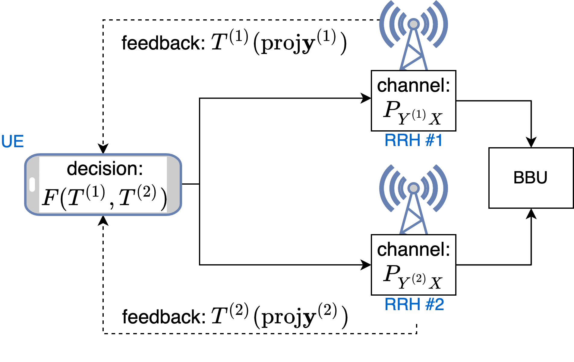
Figure 1: Uplink C-RAN scenario with local HARQ feedback generated at the RRHs which is combined at the UE.

TABLE I: Definition of parameters

Parameter	Definition
$n$	Number of modulation symbols for the decoding attempt
	at the BBU
$p$	Number of modulation symbols used at the time of
	prediction
$N_{\mathrm{b}}$	Number of bits used for feedback from RRH to UE
$T_{\mathrm{max}}$	Maximum number of transmissions/RV
$M$	Number of bits per modulation symbol, i.e. QAM
	modulation order
$N_{\mathrm{sc}}$	Number of subcode features

Fig. 1 shows the system setup which is used throughout the paper. The definitions of commonly used variables are summarized in Tab. I. We assume an uplink scenario where a UE is transmitting a packet, which is simultaneously received by two RRH. After partially receiving a packet, the RRH generate a local feedback based on the evaluated prediction algorithms. The generated local feedback is transmitted and combined at the UE. In the meanwhile, the received signals from the RRH are accumulated and jointly decoded at the BBU which determines the final decoding outcome.
Let $\mathrm{A}:=\mathbb{C}^{n}$ and $\mathrm{B}:=\mathrm{B}_{1}\times\mathrm{B}_{2}=\mathbb{C}^{p}\times\mathbb{C}^{(n-p)}=\mathbb{C}^{n}$ designate the input and output sets. Furthermore, let each channel be characterized by its respective conditional probability measure $P_{Y^{(1)}|X}:\mathrm{A}\mapsto\mathrm{B}$ and $P_{Y^{(2)}|X}:\mathrm{A}\mapsto\mathrm{B}$. Given $n$ modulation symbols, the channel probability measures represent the following association between the random vector representing the transmitted signal $X\in\mathrm{A}$ and the received signal random vectors ${Y}^{(1)},{Y}^{(2)}\in\mathrm{B}$:

$${Y}^{(i)}=\boldsymbol{H}^{(i)}X+{Z}^{(i)},\,i=1,2\,,$$ (3)

where $\boldsymbol{H}^{(i)}\in\mathrm{B}$, $i=1,2$, are random fading matrices and ${Z}^{(i)}\in\mathrm{B}$, $i=1,2$, are random noise vectors with each element distributed according to $\mathcal{CN}(0,1)$. In our link-level simulations, we assume a spatially filtered CDL channel model [29]. The assumed channel model, which is explained more in detail in Sec. III-G, can be modeled as complex channel gains that distort each symbol individually and additive normally distributed noise on top.
To determine the final decoding outcome, the BBU combines and jointly decodes the received signal vectors $Y^{(1)}$ and $Y^{(2)}$ from both RRH. On the other hand, the RRH calculate the feedback, which is a map $T^{(i)}:\mathrm{B}_{1}\to\mathrm{S}$, $i=1,2$, where $\mathrm{S}$ is the sample space of the feedback. $T^{(i)}$ is specified differently depending on the prediction scheme. As we assume binary communication, the feedback sample space reduces to $\mathrm{S}:=\mathbb{F}_{2}^{N_{\mathrm{b}}}$ where $N_{\mathrm{b}}$ is the number of bits used for the feedback transmission. Finally, the UE applies a combination rule $F:\mathrm{S}\times\mathrm{S}\to\{\mathrm{ACK},\mathrm{NACK}\}$, which leads to the corresponding UE behavior, i.e. stop transmitting or transmit more redundancy.

III Distributed early HARQ strategies

In this paper, we consider early HARQ strategies that attempt to predict the decodability of a packet ahead of the actual decoding. In particular, we take only a part of the whole transmitted signal vector into account. In contrast to early HARQ strategies that use the whole signal vector, this approach allows for providing the feedback at an earlier stage, which is crucial especially for latency-constrained use cases. In the broadest sense, the decodability prediction can be interpreted as binary statistical hypothesis testing, where the early HARQ predictor tries to discriminate between two probability distributions $P$ and $Q$: the probability distribution of decodables and the probability distribution of undecodables. The feedback maps $T^{(1)}$ and $T^{(2)}$ have to be chosen such that the two distributions become as distinguishable as possible. Ideally, these maps are sufficient statistics to the statistical hypothesis testing problem. However, in practice, depending on the type of feedback, it is a notoriously difficult problem to exactly characterize these distributions and hence, also finding sufficient feedback maps.
In terms of the system model, the prediction is based on $p$ modulation symbols with $p<n$. Hence, given $\mathrm{proj}_{p}{Y}^{(1)}$ and $\mathrm{proj}_{p}{Y}^{(2)}$, the binary hypothesis testing task at the UE is to decide between the two distributions

$$P := P_{(T^{(1)}(\mathrm{proj}_{p}Y^{(1)}),T^{(2)}(\mathrm{proj}_{p}Y^{(2)}))|D=\textrm{ACK}}$$ (4)

$$Q := P_{(T^{(1)}(\mathrm{proj}_{p}Y^{(1)}),T^{(2)}(\mathrm{proj}_{p}Y^{(2)}))|D=\textrm{NACK}}\,,$$ (5)

where $D\in\{\mathrm{ACK},\mathrm{NACK}\}$ respresents the decoding outcome at the BBU with $n$ modulation symbols available at the decoder and $\mathrm{proj}_{p}:\mathbb{C}^{k\times p}\times\mathbb{C}^{k\times(n-p)}\mapsto\mathbb{C}^{k\times p}$, $p,k,n\in\mathbb{N}$, $p<n$, denotes the function, which maps an element from the Cartesian product of two vector spaces on the first vector space.

III-A Channel-estimation-based HARQ prediction (Q-SNR)

Channel estimation predictors focus on the estimated channel realization $\boldsymbol{\hat{H}}^{(i)}$, $i=1,2$, at each RRH. The estimation is performed based on known parts of the transmitted signal, e.g. reference signals, such as DMRS. In the particular case of the paper’s transmission model, one DMRS is located at the beginning of each RV. We use these DMRS to obtain the received SNR, $\gamma^{(1)}$ and $\gamma^{(2)}$, at each RRH, respectively.

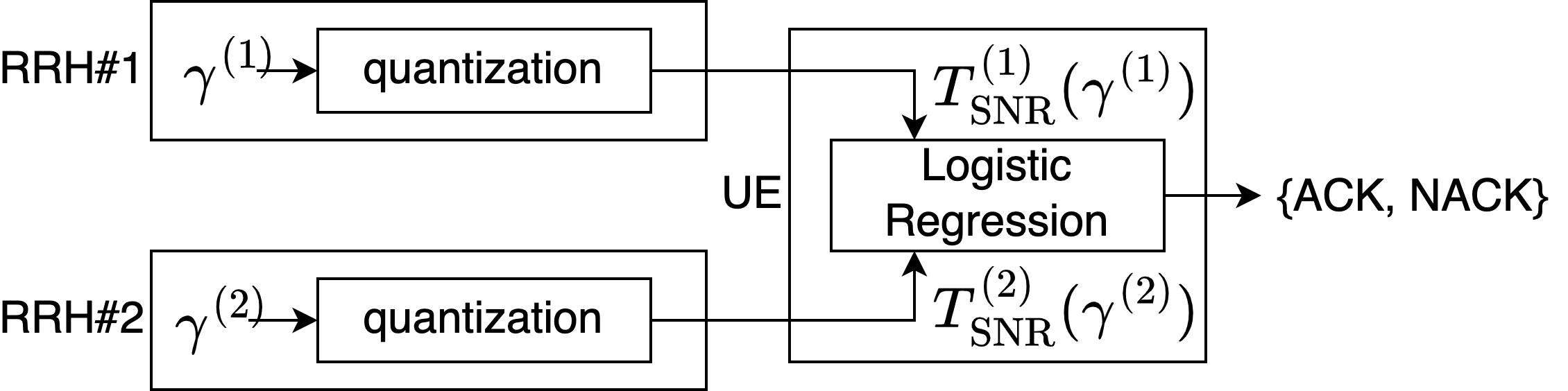
Figure 2: SNR based distributed prediction approach.

For the channel-estimation-based prediction, we evaluate the scheme proposed in [15] that accumulates the quantized received SNR from the RRH at the UE and applies a threshold to the sum to predict an ACK or NACK. In particular, $F_{\mathrm{Q-SNR}}:=T_{\mathrm{SNR}}^{(1)}+T_{\mathrm{SNR}}^{(2)}\stackunder{\stackon{\lessgtr}{\scriptstyle\mathrm{NACK}}}{\scriptstyle\mathrm{ACK}}C_{\mathrm{Q-SNR}}$, where $T_{\mathrm{SNR}}^{(i)}$, $i=1,2$, are the quantized received SNR from the respective RRH and $C_{\mathrm{Q-SNR}}$ is a constant that controls the trade-off between false-positive and false-negative errors. In the constant power case, the received SNR is equivalent to the accumulated channel gain, which is used in [15]. Furthermore, we model the quantization by a quantization layer. We assume both quantization functions $T_{\mathrm{SNR}}(\gamma):=T^{(1)}_{\mathrm{SNR}}(\gamma)=T^{(2)}_{\mathrm{SNR}}(\gamma)\forall\gamma$ to be the equal and further to be piece-wise constant functions. The constant intervals are chosen, such that each interval contains approximately the same number of data points, over the relevant SNR range, where the relevant range is determined by the minimum and maximum values of the training set. See ”quantile” in [30] for more details. Then, $T_{\mathrm{SNR}}$ assigns the value of the interval center to each SNR that falls into that interval. This scheme is designated as Q-SNR in the following. In [14] and [15], the authors use the error probability approximation from [31, Eq. (59)] to estimate the failure probability. In particular, in [14], Khalili and Simeone apply a threshold to the estimated error probability. However, in our evaluated scenario, the Q-SNR scheme achieves the same performance as the scheme in [14] at a significantly lower complexity. Hence, we restrict only to the Q-SNR scheme.

III-B LLR-based HARQ prediction (LR-LLR)

The LLR-based approaches assume that each element $x_{i}\in\mathrm{S}\subset\mathbb{C}$, $i=1,2,...,n$, of the transmitted signal vector $\boldsymbol{x}$ is i.i.d. and each element of the symbol set $\mathrm{S}$ representing $M$ bits has the same probability. We are aware that this assumption does not hold in practice due to the channel code. Nevertheless, in the next section, we discuss a scheme that does not resort to this assumption. Using the i.i.d. assumption, the LLR are calculated as

$$\Lambda_{(q-1)M+j}^{{(i)}}:=\log\frac{P(b_{(q-1)M+j}=1|r_{q})}{P(b_{(q-1)M+j}=0|r_{q})}\,,\,i=1,2\,,$$ (6)

where $r_{q}$, $q=1,2,...,n$, is the $q$-th received and equalized symbol and $b_{(q-1)M+j}$, $j=1,2,..,M$, is the $j$-th bit in the $q$-th equalized symbol. This definition of LLR leads to the following bit error probability:

$$v_{l}^{{(i)}}=\frac{1}{1+e^{|\Lambda_{l}^{{(i)}}|}}\,,l=1,2,...,p\,,\,i=1,2.$$ (7)

Against the background of [20], we provide in Eq. (7) a corrected version for the bit error probability [20, Eq. (7)].

In order to reduce the high dimensionality of $p$ bit error estimates $v_{l},l=1,...,p$, we average over all received bit error estimates:

$$\overline{v}^{(i)}:=\frac{1}{p}\sum_{l=1}^{p}v_{l}^{(i)}\,,i=1,2.$$ (8)

We apply first a local logistic regression at each RRH that is fed with $\overline{v}^{(i)}$ and the received SNR $\gamma^{(i)}$. We train the local logistic regression with the BBU decoding outcome as the ground truth. We apply $l_{2}$ regularization, see [32] for more details, and balanced weight classes to the logistic regression using the liblinear solver from the scikit-learn package [33]. The local feedback function $T_{\mathrm{LLR}}^{(i)},i=1,2,$ is given as

$$T_{\mathrm{LLR}}^{(i)}(\gamma^{(i)},\overline{v}^{(i)}):=Q\left(\frac{\exp(\theta_{20}+\begin{pmatrix}\gamma^{(i)}&\overline{v}^{(i)}\end{pmatrix}\boldsymbol{\theta}_{2})}{1+\exp(\theta_{20}+\begin{pmatrix}\gamma^{(i)}&\overline{v}^{(i)}\end{pmatrix}\boldsymbol{\theta}_{2})}\right),$$ (9)

where $Q$ is the quantization function and $\{\theta_{20}\in\mathbb{R},\boldsymbol{\theta}_{2}\in\mathbb{R}^{2}\}$ is the parameter set of the logistic regression. The quantization function $Q$ is determined analogously to the Q-SNR scheme. The range between the minimum and maximum value from the training set is divided into uniform intervals, where each interval assigns the value of its center. After having generated the local feedback $T_{\mathrm{LLR}}^{(i)}$, we again use a logistic regression at the UE to learn the feedback combination rule $F$ [34]:

$$P_{\mathrm{ACK}|T_{\mathrm{LLR}}^{(1)}T_{\mathrm{LLR}}^{(2)}}\approx P_{\mathrm{LLR}}(T_{\mathrm{LLR}}^{(1)},T_{\mathrm{LLR}}^{(2)})$$ (10)

with

$$P_{\mathrm{LLR}}(T_{\mathrm{LLR}}^{(1)},T_{\mathrm{LLR}}^{(2)}):=\frac{\exp(\theta_{30}+\begin{pmatrix}T_{\mathrm{LLR}}^{(1)}&T_{\mathrm{LLR}}^{(2)}\end{pmatrix}\boldsymbol{\theta}_{3})}{1+\exp(\theta_{30}+\begin{pmatrix}T_{\mathrm{LLR}}^{(1)}&T_{\mathrm{LLR}}^{(2)}\end{pmatrix}\boldsymbol{\theta}_{3})}\,,$$ (11)

where $\{\theta_{30}\in\mathbb{R},\boldsymbol{\theta}_{3}\in\mathbb{R}^{2}\}$ is the learnt parameter set of the logistic regression. Then, the combination rule is defined by $F_{\mathrm{LR-SNR}}(T_{\mathrm{LLR}}^{(1)},T_{\mathrm{LLR}}^{(2)}):=P_{\mathrm{LLR}}(T_{\mathrm{LLR}}^{(1)},T_{\mathrm{LLR}}^{(2)})\stackunder{\stackon{\lessgtr}{\scriptstyle\mathrm{NACK}}}{\scriptstyle\mathrm{ACK}}C_{\mathrm{LLR}}$, where $C_{\mathrm{LLR}}$ is an appropriately chosen constant. This scheme is referred to as LR-LLR.

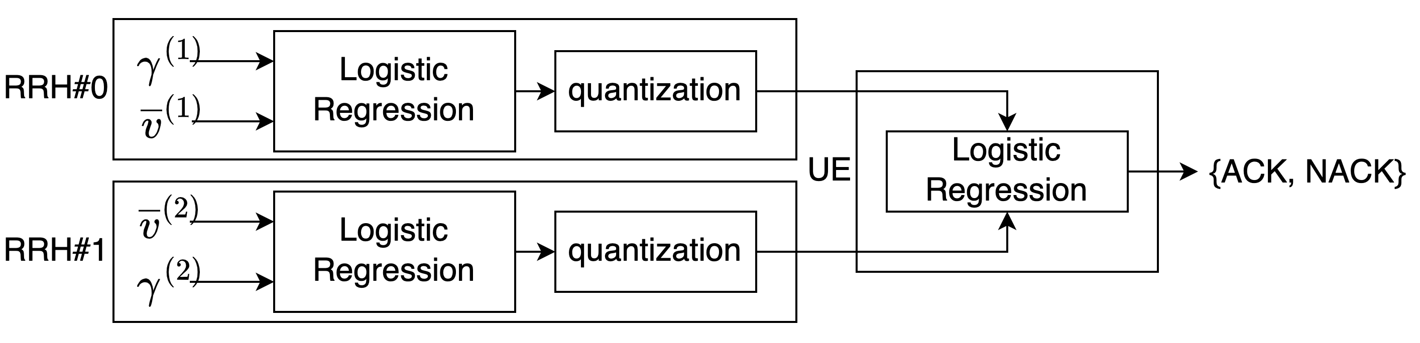
Figure 3: LR based distributed prediction approach.

III-C Subcode-based HARQ prediction

As LLR-based schemes, subcode-based HARQ predictors take the LLR as a basis. However, instead of assuming i.i.d. components of the signal vector $X$, the subcode-based prediction considers constraints defined by the parity-check matrix $\boldsymbol{P}\in\mathbb{F}_{2}^{L\times nM}$. The relation between the bit vector $\boldsymbol{b}:=(b_{i,j})\in\mathbb{F}_{2}^{nM}$, $i=1,2,...,n$, $j=1,2,...,M$, and the parity check matrix is defined as $\boldsymbol{P}\boldsymbol{b}^{\mathrm{T}}=\boldsymbol{0}$. Message passing decoders, such as the min-sum implementation, iteratively update the LLR based on $\boldsymbol{P}$, which is described by:

$$\Lambda_{l,k}^{{(i)}}=\Lambda_{l,k-1}^{{(i)}}+\sum_{m\in\mathcal{M}(l)}\delta_{m,k}^{{(i)}}\,,\,i=1,2\,,$$ (12)

where $\mathcal{M}(l)$ is the set of check nodes that are associated with the bit $b_{l}$, $\delta^{(k)}_{m,k}$ is the check node to variable node message at the $k$-th iteration, and $\Lambda_{l,k}^{(i)}$ is the updated LLR at the $k$-th iteration with $\Lambda_{l,0}^{(i)}:=\Lambda_{l}^{(i)}$. In contrast to tree codes where message passing decoders always converge to the best solution, for modern LDPC codes, the evolution of the LLR can be interpreted as a sequence which may or may not converge to a ”degraded” marginalization [35]. Compared to considering only the received LLR, this behavior provides additional information on the healthiness of the received codeword.

III-C1 Supervised dual autoencoding 2-stage gaussian mixture model (DA2SGMM) for anomaly detection

In the machine learning literature, autoencoders are well established for unsupervised anomaly detection tasks [36, 37, 38] due to their unprecedented dimensionality reduction capabilities [39]. Also for HARQ prediction purposes, a supervised autoencoder proposed in [25] outplayed other machine learning techniques, such as logistic regression, random forests, and others. However, the approach in [25], which builds on the DAGMM architecture that was proposed for anomaly detection in [37], assumes a scenario with a single receive point. In this section, we extend this autoencoder to handle two separated RRH. This novel approach, referred to as DIDA, achieves a dimensionality reduction of the input features. Furthermore, we use two independent classifiers at each RRH to convert the compressed subcode features together with the received SNR features to a decodability feedback, which is afterwards combined at the UE classifier.

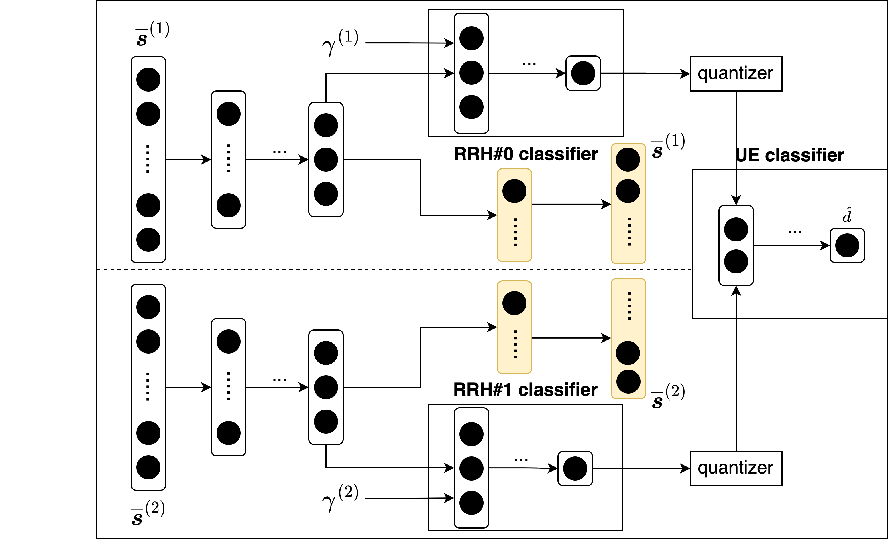
Figure 4: A supervised DIDA to compress the feedback information at the RRHs and evaluate the combined result at the UE. The yellow boxes are only used for training purposes and are removed for inference.

In Fig. 4, we show the schematic design of the proposed DIDA architecture. As can be seen, we incorporate the constraints of the architecture of the communication system directly into the setup of the DIDA. The upper box represents the parts executed at the first RRH, the lower box the parts at the second RRH and finally, the right small box represents the network at the UE. We provide further details of the DIDA setup and training in App. A.
The subcode features are generated from a partial decoding process at the RRH. In particular, the subcode features at the RRH are represented as:

$$\overline{\boldsymbol{s}}^{(i)}:=\begin{pmatrix}\overline{s}_{1}^{(i)}&...&\overline{s}_{N_{\mathrm{sc}}/4}^{(i)}\end{pmatrix}\,,i=1,2,$$ (13)

where

$$\overline{s}_{k}^{(i)}:=\frac{1}{4p}\sum_{j=1}^{4}\sum_{l=1}^{p}\frac{1}{1+e^{|\Lambda_{l,4(k-1)+j}^{(i)}|}}\,,\,k=1,...,N_{\mathrm{sc}}/4.$$ (14)

In contrast to the previous schemes, the training is performed in an end-to-end manner. Hence, we do not have to distinguish the feedback $T^{(i)}$ and the combination rule $F$. Instead, we can see the whole network, represented by $P_{\mathrm{DA2SGMM}}$, as part of the combination rule $F_{\mathrm{DA2SGMM}}\left(\overline{\boldsymbol{s}}^{(1)},\gamma^{(1)},\overline{\boldsymbol{s}}^{(2)},\gamma^{(2)}\right):=P_{\mathrm{DA2SGMM}}\stackunder{\stackon{\lessgtr}{\scriptstyle\mathrm{NACK}}}{\scriptstyle\mathrm{ACK}}C_{\mathrm{DA2SGMM}}$, where $C_{\mathrm{DA2SGMM}}$ again is a constant controlling the trade-off between false-positives and false-negatives.

III-D Complexity comparison

TABLE II: Memory consumption in number of stored floating point variables and computational complexity in terms of elementary floating point operations.

Scheme	Memory consumption	Memory consumption	Computational complexity	Computational complexity
	at the UE	at each RRH	at the UE	at each RRH
Q-SNR	1	1	$C_{\mathrm{+,*}}$	$C_{\mathrm{quant}}$
LR-LLR	$5$	$5$	$5C_{\mathrm{+,*}}+C_{\mathrm{/}}+C_{\mathrm{exp}}$	$5C_{\mathrm{+,*}}+C_{\mathrm{/}}+C_{\mathrm{exp}}+C_{\mathrm{quant}}$
DIDA	$407$	$3841$	$672C_{\mathrm{+,*}}+C_{\mathrm{/}}+C_{\mathrm{exp}}$	$7328C_{\mathrm{+,*}}+C_{\mathrm{/}}+C_{\mathrm{exp}}+C_{\mathrm{quant}}$

The different HARQ prediction strategies come at different costs in terms of computations and memory. In particular, the required processing time, which results from the computational complexity, is critical for low-latency applications. In order to compare the different schemes, we assume that the SNR and LLR features themselves are available without any processing cost. In [40], the decoding latency of a flexible offset min-sum LDPC decoder is given by

$$\delta_{\mathrm{dec}}=\left\lceil\frac{Nd_{v}}{Z}\right\rceil\frac{I}{f}\,,$$ (15)

where $N$ is the size of the codeword, $d_{v}$ is the average variable node degree, $Z$ is the lifting size of the code, i.e. 104, $I$ is the number of performed iterations and $f$ is the clock rate of the decoder. This decoder type is implementation-wise very similar to the optimized min-sum LDPC algorithm, which has been used for the simulations. Applying to the used subcode and assuming a decoder frequency of 1 GHz, as motivated in [40], we obtain a decoding latency of 305 ns for the partial decoding to obtain the subcode features from the LLR.

For the evaluation of the classifiers, we determine the amount of memory required to store the model parameters and input features and the number of elementary floating-point operations. Furthermore, to validate the estimated we perform a processing time measurement of a single-threaded implementation of the schemes on an Intel(R) Xeon(R) CPU E5-2687W v3 @ 3.10GHz processor. The LR-LLR scheme uses logistic regressions with 2 input features each. Hence, besides the features themselves, the parameter set of the logistic regression also has to be stored on the devices. This results to a memory consumption of $C_{\mathrm{mem},\mathrm{LR}}=5$. Furthermore, the computational complexity is given by $C_{\mathrm{comp},\mathrm{LR}}=5C_{\mathrm{+,*}}+1C_{\mathrm{/}}+1C_{\mathrm{exp}}$, where $C_{\mathrm{+,*}}$ is the computational complexity of an elementary multiplication or addition, $C_{\mathrm{/}}$ is the computational complexity of an elementary division and $C_{\mathrm{exp}}$ is the complexity of computing the exponential function. We use $C_{\mathrm{quant}}$ to designate the computational complexity of the quantization. Different from the logistic regression, the DIDA scheme is built up by multiple FC layers, see App. A for more details. The overall memory consumption of an FC layer results to

$$C_{\mathrm{mem},\mathrm{FC}}=(N_{\mathrm{in}}+3)N_{\mathrm{out}}\,.$$ (16)

Furthermore, the overall computational complexity of an FC layer is given by

$$C_{\mathrm{comp},\mathrm{FC}}=2N_{\mathrm{out}}(N_{\mathrm{in}}+1)C_{\mathrm{+,*}}\,.$$ (17)

The Softmax layer does not have any stored parameters and hence, $C_{\mathrm{mem},\mathrm{SM}}=0$. The computational complexity is given by $C_{\mathrm{comp},\mathrm{SM}}=2C_{\mathrm{+,*}}+1C_{\mathrm{/}}+1C_{\mathrm{exp}}$.

TABLE III: Single-threaded processing time on different processor platforms.

Scheme	Device	Number of	Estimated processing time	Actual processing time
		operations	Raspberry Pi 3 Model B	Intel(R) Xeon(R) CPU E5-2687W v3 @ 3.10GHz
			approx. 4 GFLOPS [41]	approx. 49.6 GFLOPS, obtained from linpack
Q-SNR	UE	1	0.3 ns	0.4 ns
Q-SNR	RRH	4	1.0 ns	24.4 ns
LR-LLR	UE	17	4.3 ns	72.8 ns
LR-LLR	RRH	21	7.0 ns	158.5 ns
DIDA	UE	692	173.0 ns	102.1 ns
DIDA	RRH	7351	1837.8 ns	519.0 ns

TABLE IV: Estimated parallelized processing time of DA2SGMM on a Raspberry Pi 3 platform.

Number	Device	Number of	Scaling	Estimated processing time
of cores		operations	factor	Raspberry Pi 3 Model B
		per core		approx. 4 GFLOPS
				(per core) [41]
8	UE	103	6.72	25.8 ns
8	RRH	949	7.75	237.3 ns
16	UE	85	8.14	21.3 ns
16	RRH	536	13.71	134.0 ns

Tab. II summarizes the overall complexity of all schemes. Obviously, the Q-SNR scheme has the least memory consumption as well as the least computational complexity at all devices. Compared to that, the LR-LLR slightly increases the memory consumption and computational complexity at the RRH. The DIDA clearly has the highest memory consumption and computational complexity on all devices. The complexity of the elementary operations can be approximated by weights corresponding to the number of performed floating point operations: $C_{\mathrm{+,*}}:=1$, $C_{\mathrm{/}}=4$ and $C_{\mathrm{exp}}=8$ [42]. For the quantization, we take PyTorch’s FakeQuantize implementation as baseline [43]. Hence, the computational complexity of the quantization results to $C_{\mathrm{quant}}=4C_{\mathrm{+,*}}$. Tab. III shows the estimated processing times for a Raspberry Pi 3 processor and the results of actual processing time measurements on an Intel Xeon processor. In a practical implementation, the processing time may vary based on the capabilities of the processor platform, the latency of memory access, the efficiency of the implementation and many more factors. However, this impact also heavily depends on the actual implementation. This also explains discrepancies between the estimated processing times and the actual processing times. Obviously, the quantization operation requires much more time on the Intel processor than estimated. In contrast to the DIDA that uses PyTorch also for the quantization, we use scikit-learn’s KBinsDiscretizer for the quantization of the other schemes. Also, the implementation of the linear regression is not optimized for the particular case and hence, performs unnecessary double calculations. Furthermore, we do not consider memory access delays for our estimated processing times. However, with specialized hardware, such as GPUs or even TPUs, a significantly better performance is to be expected. In Tab. IV, we show a simple estimation of the processing times of the DIDA on multi-core platforms. We assume that matrix multiplications resulting in an output vector, i.e. a linear layer, can easily be parallelized by computing each entry of the output vector separately. We observe that the processing time on the RRH scales almost linearly up to 16 cores. In contrast to that, on the UE, 16 cores only have a very small advantage compared to 8 cores. However, a UE processing time of 25.8 ns already is very small. Nevertheless, the processing times are at most in the small µs range on single-threaded platforms, which is extremely small even compared to stringent latency budgets, such as 1 ms and even 0.1 ms. In particular, specialized hardware, such as GPUs and TPUs, are widely used to run neural networks. Overall, our evaluation shows that the processing time are expected to be sufficiently small on practical platforms.

III-E Data transmission model

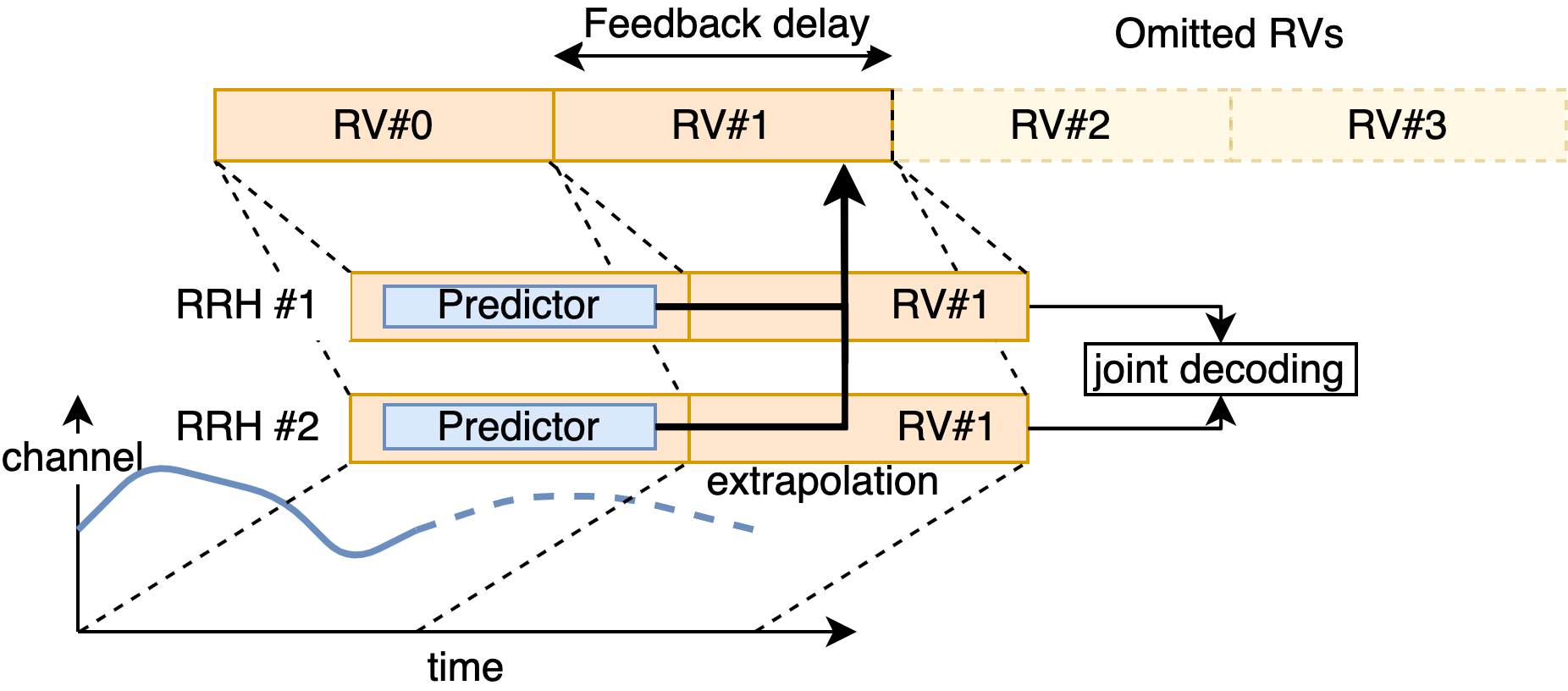
Figure 5: Data transmission model incorporating the feedback delay.

We assume an incremental redundancy HARQ protocol with up to four RV. In our simulation setup, an RV spans over 14 OFDM symbols in time, which is equivalent to 15.63 µs. The UE transmits the RV in a consecutive manner, as depicted in Fig. 5. After receiving each RV, the RRH provide feedback using the previously described prediction schemes. The UE decides based on a combination rule $F$ whether further RV are required or not. This approach enables a good trade-off between reliability and spectral efficiency since some RV are omitted, if an early decoding is successfully predicted. After having received all RV from the UE, the RRH forward the received signals to the BBU where a single decoding attempt is conducted. In this work, we simulate four RV; hence, there are three prediction points:

1. the first prediction point (Pos#1), which uses the received RV#0 to decide whether RV#2 is required or not,

2. the second prediction point (Pos#2), which uses RV#0 and RV#1 to decide whether RV#3 is required or not.

3. the blockage prediction point (Pos#3), which uses RV#0-2 to decide whether blockage is detected or not.

A positive prediction at the first prediction point causes the UE to stop transmitting further RV. Hence, the second prediction point would not be reached in that case. However, this depends on the particular prediction scheme and modeling this accurately would require to incorporate the prediction directly into the link-level simulations, which increases the complexity extremely. Instead, we assume that all prediction schemes correctly identify transmissions that are already decodable with the first RV and only the remaining transmissions reach the second prediction point.

III-F Evaluation methodology

In addition to achieving the reliability and the latency targets which are mandatory requirements, the performance of the HARQ prediction schemes can be compared in terms of their achieved throughput. In contrast to commonly used classifier performance metrics, such as precision and recall, the throughput provides a measure with direct takeover to practical scenarios. Especially, when considering edge cases with extremely low-reliability requirements, common classifier metrics may not provide a good metric for comparison [25].
Based on the renewal-reward theorem [44], the throughput is expressed as $\eta=\frac{\mathbb{E}[\mathcal{R}]}{\mathbb{E}[L(T)]}$, where $\mathbb{E}[\mathcal{R}]$ is an expected reward and, $\mathbb{E}[L(T)]$ is the expected transmission latency with $L(T)$ as defined in (18) and (19) and $T\in\mathbb{N}^{+}$ being the number of requested RV. Furthermore, the reward is $\mathcal{R}:=0$ in case the transmission failed within the latency budget. In case the transmission was successful, $\mathcal{R}$ is $N_{\mathrm{packet}}$, the size of the packet in nats. Hence, the expected reward is given as $\mathbb{E}[\mathcal{R}]:=(1-\epsilon_{\mathrm{tot}})N_{\mathrm{packet}}$, where $\epsilon_{\mathrm{tot}}$ is the associated total error probability. The transmission latency of the prediction schemes is composed of multiple components:

$$L_{\mathrm{e}}(T)=\begin{cases}\!\begin{aligned} &T\delta_{\mathrm{RV}}+(T-1)\delta_{\mathrm{exc}}\end{aligned}&\text{if }1\leq T\leq T_{\mathrm{max}}\\ \!\begin{aligned} &T_{\mathrm{max}}\delta_{\mathrm{RV}}+L_{\mathrm{blk}}\\ &+(T_{\mathrm{max}}-1)\delta_{\mathrm{exc}}\end{aligned}&\text{if }T>T_{\mathrm{max}}\end{cases}\,,$$ (18)

where $\delta_{\mathrm{exc}}:=\max(\delta_{\mathrm{proc}}+\delta_{\mathrm{fb}}-\delta_{\mathrm{RV}},0)$ and $\delta_{\mathrm{RV}}$ is the time to transmit an RV, $\delta_{\mathrm{proc}}$ is the processing time required by the specific prediction scheme and $\delta_{\mathrm{fb}}$ is the time required to transmit the feedback. Furthermore, $L_{\mathrm{blk}}$ is a latency penalty. For simplicity, we assume $L_{\mathrm{blk}}=T_{\mathrm{blk}}\delta_{\mathrm{RV}}$, where $T_{\mathrm{blk}}$ is a spectral efficiency penalty when blockage is detected. In contrast to that, the latency of a regular HARQ system is composed as:

$$L_{\mathrm{r}}(T)=\begin{cases}T\delta_{\mathrm{RV}}+(T-1)(\delta_{\mathrm{fh}}+\delta_{\mathrm{fb}})&\text{if }1\leq T\leq T_{\mathrm{max}}\\ \!\begin{aligned} &T_{\mathrm{max}}\delta_{\mathrm{RV}}+L_{\mathrm{blk}}\\ &+(T_{\mathrm{max}}-1)(\delta_{\mathrm{fh}}+\delta_{\mathrm{fb}})\end{aligned}&\text{if }T>T_{\mathrm{max}}\end{cases}\,,$$ (19)

where $\delta_{\mathrm{fh}}$ is the fronthaul round-trip time, which is the time required for transporting the received signal vectors to the BBU, decoding the packet at the BBU, and sending the result back to the RRH.
The probability distribution of $T$ for a feedback delay of $\delta:=1$ is determined by the performance of the different estimators:

$$\mathbb{P}[T=t]=\begin{cases}\!\begin{aligned} &p_{t-2}\epsilon_{t-1}\alpha_{t-1}\\ &+p_{t-2}(1-\epsilon_{t-1})\\ &\cdot(1-\beta_{t-1})\end{aligned}&\text{if }2\leq t\leq T_{\mathrm{max}}\\ p_{T_{\mathrm{max}}-1}&\text{if }t=T_{\mathrm{max}}+T_{\mathrm{blk}}\\ 0&\text{otherwise}\end{cases}$$ (20)

with

$$p_{t}:=\prod_{j=1}^{t}\epsilon_{j}(1-\alpha_{j})+(1-\epsilon_{j})\beta_{j}\,,$$ (21)

where $T_{\mathrm{max}}$ is the maximum number of transmissions, $T_{\mathrm{blk}}$ is an additional spectral efficiency penalty in case blockage is detected, $\epsilon_{j}$, $j\in\{1,2,...,T_{\mathrm{max}}-1\}$, are the error probabilities at the $(j+1)$-th RV given that previous RV were unsuccessful, $\alpha_{j}$, $j\in\{1,2,...,T_{\mathrm{max}}-1\}$, are the false positive probabilities, i.e. predicting an unsuccessful decoding as an ACK, and $\beta_{j}$, $j\in\{1,2,...,T_{\mathrm{max}}-1\}$, are the false negative probabilities, i.e. predicting a successful decoding as a NACK. The false-positive and false-negative probabilities are defined as

$$\alpha_{j}:=P_{D_{j+1}=\mathrm{NACK}|F_{j}=\mathrm{ACK}}\,,$$ (22)

and

$$\beta_{j}:=P_{D_{j+1}=\mathrm{ACK}|F_{j}=\mathrm{NACK}}\,,$$ (23)

where $D_{j+1}$ is the decoding outcome with $(j+1)$ RV and $F_{j}$ is the outcome of the $j$-th prediction.
The total error performance $\epsilon_{\mathrm{tot}}$ is determined by the error probabilities $\epsilon_{i}$ but also the false positive error probability $\alpha_{i}$. The total error performance in a non-blockage scenario is given by [10]:

$$\epsilon_{\mathrm{tot}|\mathrm{nb}}=\left(\sum_{t=1}^{T_{\mathrm{max}}-2}\left(\prod_{j=1}^{t-1}\epsilon_{j}(1-\alpha_{j})\right)\epsilon_{t}\alpha_{t}\right)\\ +\left(\prod_{i=1}^{T_{\mathrm{max}}-2}\epsilon_{i}(1-\alpha_{i})\right)\epsilon_{T_{\mathrm{max}}-1}\,,$$ (24)

where the false-positive, false-negative and error probabilities are estimated from non-blockage scenarios. However, in a blockage scenario a sufficiently low error probability cannot be maintained and hence, alternative procedures, e.g. additional redundancy, switching to a lower frequency or adapting the beam, have to be initiated. However, instead of making an assumption on the specific blockage recovery scheme, we use the spectral efficiency penalty $T_{\mathrm{blk}}$ to model the blockage case. This also means that an effective blockage, i.e. non-decodability of the $T_{\mathrm{max}}$ RV, has to be detected with the same target error probability. The probability of blockage misdetection is given by

$$\epsilon_{\mathrm{blk}|\mathrm{sb}}=\left(\sum_{t=1}^{T_{\mathrm{max}}-3}\left(\prod_{j=1}^{t-1}\epsilon_{j}(1-\alpha_{j})\right)\epsilon_{t}\alpha_{t}\right)\\ +\left(\prod_{j=1}^{T_{\mathrm{max}}-3}\epsilon_{j}(1-\alpha_{j})\right)\epsilon_{T_{\mathrm{max}}-1}\alpha_{T_{\mathrm{max}}-1}\,,$$ (25)

where the false-positive, false-negative and error probabilities are derived from single-blockage scenarios.
The false-positive probabilities and the false-negative probabilities behave in a conflicting manner, where the trade-off between both can be controlled by adjusting the bias $s$ of the respective predictor. However, the functional relation between $\alpha_{i}(s)$ and $\beta_{i}(s)$, $i=1,...,T_{\mathrm{max}}-1$, is not known. Hence, we determine 1000 admissible pairs $(\alpha_{i}(s_{j}),\beta_{i}(s_{j}))$, $j=1,2,...,1000$, from the link-level simulations and interpolate them piece-wise linearly. Obviously, any false-positive false-negative curve of a reasonable predictor is a convex function, where at the extreme case when no prediction is possible, this function becomes a straight line connecting the points $(0,1)$ and $(1,0)$. Hence, a piece-wise linear interpolation is a conservative approximation, where the actual performance of the predictors at an interpolated point is expected to be better than the approximated value.

With $\boldsymbol{s}:=(s_{1},s_{2},...,s_{T_{\mathrm{max}}-1})$ being the vector of biases per prediction, we derive the following optimization problem for the expected number of RV under no blockage:

$$\underset{\boldsymbol{s}}{\text{minimize}} \mathbb{E}[T(\boldsymbol{\alpha}_{\mathrm{nb}}(\boldsymbol{s}),\boldsymbol{\beta}_{\mathrm{nb}}(\boldsymbol{s}))]$$ (26)

subject to $$\epsilon_{\mathrm{tot|nb}}(\boldsymbol{\alpha}_{\mathrm{nb}}(\boldsymbol{s}))\leq\epsilon_{\mathrm{target}}$$

and $$\epsilon_{\mathrm{blk|sb}}(\boldsymbol{\alpha}_{\mathrm{sb}}(\boldsymbol{s}))\leq\epsilon_{\mathrm{target}}\,,$$

where $\epsilon_{\mathrm{target}}$ corresponds to the overall reliability requirement. We use the SLSQP algorithm [45] with a Monte-Carlo approach to numerically find a valid solution to the aforementioned optimization problem.

III-G Link-level simulation setup

TABLE V: Link-level simulation assumptions for training, hyper and test set generation.

TB size	1000
in bits ($N_{\mathrm{Bits}}$)
RV length in bits	2016
RV duration ($\delta_{\mathrm{RV}}$)	14 OFDM symbols $\hat{=}$ 15.625 µs
Transmission configuration	$T_{\mathrm{max}}=4$, $\delta_{\mathrm{fb}}=1$
Transmission bandwidth	40.0 MHz (6 PRBs)
Channel Code	5G LDPC (see [46])
Modulation order and algorithm	4-QAM, $M=2$, Approximated LLR
Power allocation	Constant $E_{b}/N_{0}$
Waveform	3GPP OFDM, normal cyclic-prefix,
	960 kHz subcarrier spacing
SNR range	no-blockage:
	4.0 dB, 5.0 dB, 6.0 dB, 7.0 dB
	single-blockage:
	-7.2 dB, -6.2 dB, -5.2 dB, -4.2 dB
Target error rates $\epsilon_{\mathrm{target}}$	$1\cdot 10^{-4}$ (4 dB), $3.5\cdot 10^{-5}$ (5 dB),
	$1\cdot 10^{-5}$ (6 dB), $3.5\cdot 10^{-6}$ (7 dB)
Channel type (no-blockage)	filtered CDL-D 30 ns (Rician LOS),
	directional Rx/Tx antenna pattern,
	100 GHz, 50 km/h,
	ideal channel estimation
Channel type (single-blockage)	filtered CDL-C 30 ns (Rayleigh LOS),
	directional Rx/Tx antenna pattern,
	100 GHz, 50 km/h,
	ideal channel estimation
Equalizer	Frequency domain MMSE
Decoder type	Min-Sum (50 iterations)

To compare the performance of previously described HARQ prediction schemes, we conduct link-level simulations to collect the required LLR, subcode and channel estimation features. We choose the frame structure of the transmission, i.e. the mapping of the code block to resource elements and reference signals, e.g. DMRS, in accordance with the Rel. 16 3GPP specifications. Furthermore, we use a subcarrier spacing of 960 kHz, which is currently being specified in the ”NR operation up to 71 GHz” work item [1]. Tab. V summarizes the link-level parameters. We assume that different UE are scheduled on different orthogonal time-frequency resources and hence, interference from other transmitters can be neglected. In the sub-THz frequency spectrum, the use of beamforming is necessary due to the high pathloss, even for free space propagation. However, MIMO schemes that allow dynamic beamforming are complex in the sense that they offer a large set of tunable parameters and transmission modes. Optimizing these goes beyond the scope of this work. Hence, we use a spatially filtered CDL-D channel model that already incorporates the effects of beamforming [29], see Sec. III-G for more details.
We evaluate the performance in a single-blockage and a no-blockage scenario. We do not consider the case where both RRH are blocked, as this would also make any communication at a feasible rate impossible. In the no-blockage scenario, we assume no SNR difference between the two RRH. In the single-blockage scenario, we assume the same SNR at the non-blocked RRH and an additional pathloss of 11.2 dB at the blocked RRH. This is the pathloss difference of a blocked and non-blocked channel with a UE at 20 m distance from both RRH in the UMi scenario [29]. At the RRH, we use a spatially filtered CDL channel model. In particular; at the un-blocked RRH, we use CDL-D, which is a LOS channel model with Rician distributed LOS component and Rayleigh distributed NLOS components [29]. At the blocked RRH, we use the CDL-C, which is a NLOS channel model [29]. Furthermore, we apply the directional antenna pattern, as specified in [47], at both sides to generate a spatially filtered TDL channel which models the effective channel between the UE and the RRH. The spatial filtration procedure is performed in accordance with [29, Sec. 7.7.4]. For the decoding of the received signal vector, we apply an optimized min-sum algorithm [48] with 50 iterations. In contrast to that, the subcode prediction uses only 5 iterations. Hence, its complexity is only 1/10-th of the complexity of a full decoding attempt.

IV Simulation Results

In this section, we present the results for the different HARQ prediction approaches. We train all schemes jointly on all SNR except 6 dB. The SNR of 6 dB is not used during training but only used for testing to evaluate the generalization performance of the models.

IV-A False-positive and false-negative performance

The false-positive and false-negative mispredictions determine the performance of the predictor, as we can see from Eq. (20) and (24). Especially, the regime of low false-positives is of special interest because the cost of a false-positive misprediction is significantly higher than the cost of a false-negative misprediction. However, due to the finite size of the test sets, we have to deal with false-positives of zero, which makes a logarithmic scale unusable. Hence, a symmetrical logarithmic scale has been chosen for the false-positive axis. This scaling puts emphasis on the lower regime of the false-positive probabilities while keeping the zero point interpretable; however, special care has to be given to the linear scaling between the zero and the first step.

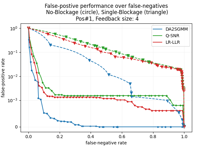
(a)

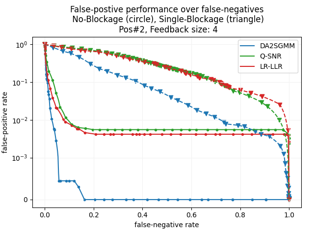
(b)

Figure 6: False-positive prediction performance over false-negatives after the first RV and after second RV with 4 bit feedback. No-blockage (circle). Single-blockage (circle). (a) First prediction point. (b) Second prediction point.

Fig. 6 shows the SNR-averaged false-positive rate over the false-negative rate at the first and the second prediction points with a feedback size of 4 bits. In Fig. 6a, we note that all schemes achieve a better performance in the no-blockage scenario compared to the single-blockage scenario. In particular, the Q-SNR and LR-LLR achieve in both scenarios a comparable performance, whereas the LR-LLR performs slightly better than the other schemes except at very small false-negative rates in the no-blockage scenario. Furthermore, we note that the DIDA clearly outperforms all other schemes in both scenarios. In the no-blockage scenario, it reaches zero mispredictions on the test set already at an false-negative rate of approximately $0.5$. In contrast to that, the other schemes reach zero mispredictions only at a false-negative rate of $1$. This behavior even reinforces at the second prediction point, seen in Fig. 6b. Here, in the no-blockage scenario, the DIDA reaches zero mispredictions already below a false-negative rate of $0.2$. In the single-blockage scenario, the performance of the DIDA degrades slightly compared to the first prediction point. However, the performance of the other prediction schemes degrades significantly in both scenarios compared to the first prediction point.

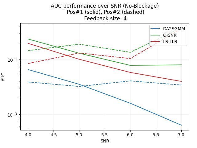
(a)

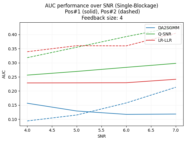
(b)

Figure 7: AUC performance over SNR with a feedback size of 4 bits. First prediction point (solid). Second prediction point (dashed). (a) No-blockage scenario. (b) Single-blockage scenario.

The false-positive-false-negative curve only shows the averaged performance. Hence, we also want to compare the performance of the schemes at specific SNR. In particular, the SNR of 6 dB is of uttermost interest as this data was excluded from the training. Hence, we further introduce the notion of the AUC as $AUC:=\int_{0}^{1}\tilde{f}_{\boldsymbol{\alpha},\boldsymbol{\beta}}(x)dx$, where $\tilde{f}_{\boldsymbol{\alpha},\boldsymbol{\beta}}(x)$ is the piece-wise linear interpolation of the false-positive-false-negative pairs $(\boldsymbol{\alpha},\boldsymbol{\beta})$. In Fig. 7, we present the AUC performance in the no-blockage and single-blockage scenarios with a feedback size of 4 bits. In the no-blockage scenario, in Fig. 7a, we observe at the first prediction point that the AUC decreases with increasing SNR, i.e. the prediction accuracy increases. In particular, for the SNR of 6 dB, we note that none of the schemes show a particularly degraded AUC performance. For the second prediction point, we observe that the AUC tends to slightly increase with increasing SNR for all schemes except the DIDA, which shows an almost flat behavior over the SNR range. As seen already in Fig. 6, it can be clearly seen that the DIDA achieves by far the lowest AUC at all SNR and both prediction points. In the single-blockage scenario, in Fig. 7b, we observe the AUC tending to increase with the SNR except for the DIDA at the first prediction point. Again, the DIDA clearly outperforms the other schemes at all SNR and both prediction points. Furthermore, we note as in the no-blockage scenario that no degradation of the AUC at an SNR of 6 dB can be observed. Hence, a good generalization of all models may be assumed.

IV-A1 Impact of feedback size

In the previous section, we show results for a feedback size of 4 bits. However, the question of how many feedback bits are required is important for the practicability of the HARQ prediction schemes, as more bits result in a significantly higher control signaling overhead.

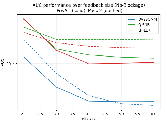
(a)

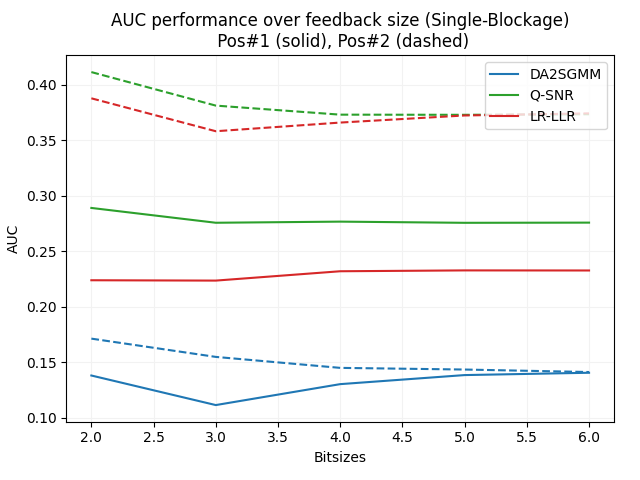
(b)

Figure 8: Averaged AUC performance over different feedback sizes. First prediction point (solid). Second prediction point (dashed). (a) No-blockage scenario. (b) Single-blockage scenario.

In Fig. 8, we show the SNR-averaged AUC over different feedback sizes in the no-blockage and the single-blockage scenarios, in Fig. 8a and Fig. 8b, respectively. In the no-blockage scenario, Fig. 8a, we clearly note a trend of lower AUC at higher feedback sizes. This matches the intuition that more accurate feedback benefits the prediction accuracy. However, in the single-blockage scenario, in Fig. 8b, we observe a lower AUC at lower feedback sizes. Although this seems counter-intuitive, this behavior is explained by the trade-off between the no-blockage AUC and the single-blockage AUC. Depending on the hyperparameters, the feedback size itself and in particular the ACK weight class for the DIDA, see Sec. A, the schemes train for a different trade-off at the different feedback sizes. Besides that, we observe that the DIDA achieves the lowest AUC at both prediction points and in both scenarios even compared to higher feedback sizes of the other schemes. Furthermore, we can see that all schemes profit from more feedback bits. In particular, we observe that Q-SNR gains the most until 3 bits and only benefits slightly from more bits. The LR-LLR and DIDA mostly improve in terms of AUC until 4 bits. Although, the DIDA has an outlier for the first prediction point at 3 bits in the blockage scenario, as seen in Fig. 8b.

IV-A2 Blockage Detection

In addition to the first and second HARQ prediction points, the blockage prediction also plays a crucial role for practical applications.

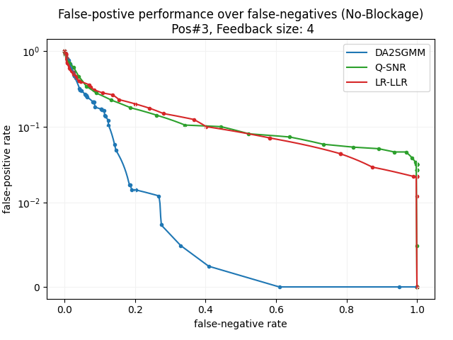
(a)

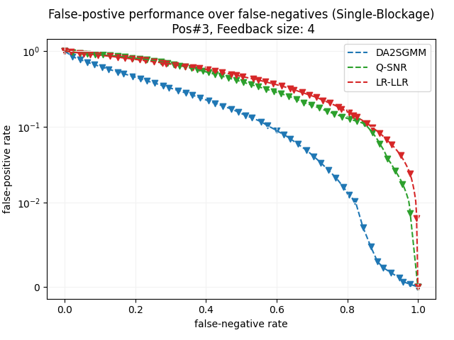
(b)

Figure 9: Blockage prediction at the third prediction point with a feedback size of 4 bits. (a) No-blockage scenario. (b) Single-blockage scenario.

In Fig. 9, we show the SNR-averaged false-positive rate over the false-negative rate in the no-blockage and the single-blockage scenarios, in Fig. 9a and Fig. 9b, respectively. Similar to the previous prediction points, we observe generally a better performance for all schemes in the no-blockage scenario compared to the single-blockage scenario. Again, the DIDA clearly achieves a significantly lower false-positive rate at the same false-negative rates. These results indicate a superior performance for the DIDA scheme compared to the other schemes in terms of HARQ prediction and also blockage detection.

IV-B HARQ system performance

In the previous section, we evaluated the false-positive and false-negative performance. However, the performance in a practical setup has to be shown to prove the efficiency of a scheme. Hence, we evaluate the different prediction schemes using the evaluation methodology described in Sec. III-F.

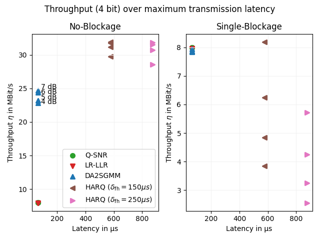
(a)

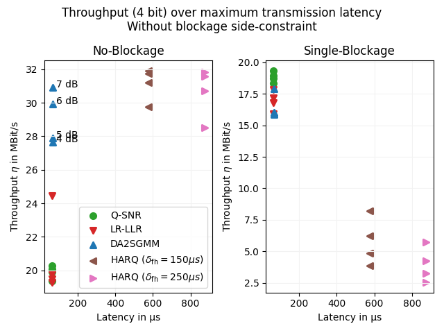
(b)

Figure 10: Throughput (4 bits feedback) over the maximum transmission latency ($\delta_{\mathrm{fb}}=\delta_{\mathrm{RV}}$) with and without the blockage side constraint at the evaluated SNR and corresponding target error rates, as provided in Tab. V. (a) With blockage constraint. (b) Without blockage constraint.

In Fig. 10, we show the HARQ performance of the prediction schemes with 4 bits feedback size in terms of the throughput with and without the blockage side constraint as defined in (26). We assume $T_{\mathrm{blk}}:=4$, which implies that a positive blockage detection results in 4 additionally requested RV. Furthermore, we set $\delta_{\mathrm{fb}}=\delta_{\mathrm{RV}}$. Due to the downlink control signaling design, i.e. PDCCH in 5G, it is possible to achieve even smaller feedback delays. However, as it is clear from (18), any smaller $\delta_{\mathrm{fb}}$ would diminish the impact of the complexity differences of the schemes. For the processing latency of the schemes, we take the measurement results from the single-threaded implementation on an Intel Xeon CPU as a basis. In Fig. 10a, we observe in the no-blockage scenarios that DIDA with 23 - 25 Mbit/s throughput clearly outperforms all other prediction schemes, which achieve approximately 8 MBit/s at all SNR. We note that the latency that is required to achieve the target error rates, does not differ significantly for the HARQ prediction schemes. Compared to regular HARQ, DIDA reaches approximately 20 % less throughput. Nevertheless, the higher throughput of regular HARQ comes at the cost of a significantly larger maximum transmission latency compared to DIDA. In the single-blockage scenario, we note that the additional latency due to retransmissions significantly degrades the throughput of regular HARQ. The DIDA, Q-SNR and LR-LLR achieve a similar and significantly higher throughput for all SNR except the 7 dB SNR of HARQ with $\delta_{\mathrm{fh}}=150\mu s$. In Fig. 10b, we show the throughput without the blockage side constraint. We observe that the performance improves for all prediction schemes in both scenarios. Especially, the Q-SNR and LR-LLR significantly benefit from removing this side constraint. This indicates that in the previous performance evaluations, these schemes are mainly limited by the stringent blockage detection side constraint defined in (26).
Another critical issue for machine learning schemes is the robustness against unknown channel variations. In particular, any learned scheme has to reliably perform for a larger range of channel parameters, such as the SNR. In order to test the robustness of the trained DIDA, we exclude the SNR of 6 dB from training. We note that the throughput of DIDA behaves as expected also at this SNR point. Furthermore, we note that the achieved throughput at 6 dB is even closer to the throughput of 7 dB than 5 dB, which hints that the scheme behaves as expected also in unknown channel variations.

V Summary and Conclusions

In this work, we proposed novel machine-learning assisted HARQ prediction schemes and evaluated them within the context of a C-RAN scenario in the sub-THz regime consider also blockage using link-level simulations. In particular, we extended the LLR- and subcode-based approaches proposed in [25] enabling their usage in a C-RAN setup by introducing quantization and a feedback combination module using a logistic regression and we proposed a novel end-to-end DIDA architecture that exploits SNR and subcode features. Using realistic link-level simulations, we showed that the proposed DIDA clearly outperforms other prediction mechanisms in no-blockage as well as in single-blockage scenarios within the context of the HARQ evaluation methodology. In particular, we present that the DIDA HARQ prediction achieves a more than 200 % higher throughput compared to other HARQ prediction schemes at SNR ranging from 4 dB to 7 dB and target error rates from $1\cdot 10^{-4}$ to $3.5\cdot 10^{-6}$, if single-blockage is considered. Even without blockage, we show that the throughput of the DIDA is approx. 29 % higher compared to the LR-LLR and even 45 % higher compared to the Q-SNR. Compared to regular HARQ, our proposed DIDA with a sufficient feedback size suffers only by a throughput reduction of approx. 20 % while reducing the maximum transmission latency by a factor larger than 4. Furthermore, we show that 4 bits for the feedback transmission is sufficient and the schemes do not benefit from more bits. In future research, the impact of double-blockage as well as a setup with more than two RRH may be studied. Furthermore, the impact of non-ideal channel estimation on the performance of the different schemes has to be evaluated in further studies.

Appendix A Dual-Input Denoising Autoencoder

The network configuration for the encoders at each RRH is [FCL($d$,25), FCL(25,10), FCL(10,3)] and for the decoder [FCL(3,15), FCL(15,40), Lin(40,$d$)], where FCL(x,y) $\equiv$ [Lin(x,y), BN, L-ReLU] and $d$ is the input dimension. Furthermore, Lin(x,y) denotes a linear transformation layer, BN a Batch Normalization-layer, L-ReLU a Leaky ReLU activation layer with a slope of $0.01$. Each RRH further contains a classifier that operates on the compressed form of the subcode features. The network configurations of the RRH classifiers each read as [FC(5,10), FC(10,15), FC(15, 15), FC(15, 10), Lin(10, 2), SM], where FC(x,y) $\equiv$ [Lin(x,y), BN, ReLU] where ReLU is a ReLU activation layer and SM is a softmax activation layer. The classifiers each receive the compressed representation of $\overline{\boldsymbol{s}}^{(i)}$ and the received SNR $\gamma^{(i)}$ as input. To prevent drifting off of the two ”arms” of the network, the local encoders and classifiers are tied together. In particular this means, the weights and the biases of the linear layers are updated equally at both RRH. Furthermore, we implement the quantization layer by a FakeQuantize layer with a MinMaxObserver in PyTorch using quantization-aware training [49]. Lastly, the network configuration of the UE classifier is given by [FC(2,20), FC(20,10), FC(10,5), Lin(5,2), SM]. We train the DIDA in an end-to-end fashion using a loss function $L$ that is composed by the $L_{2}$ norm:

$$L_{2}=\frac{1}{N}\sum_{i=1}^{2}\sum_{k=1}^{N}||\boldsymbol{s}^{(i)}_{k}-\hat{\boldsymbol{s}}^{(i)}_{k}||_{2}^{2}\,,$$ (27)

and the cross-entropy between the predicted output $\hat{d}$ and the actual decoding outcome $d$:

$$L_{\mathrm{ce}}=\frac{1}{1+\omega_{\mathrm{ACK}}}\left(d_{k}\log(\hat{d}_{k})+\omega_{\mathrm{ACK}}(1-d_{k})\log(1-\hat{d}_{k})\right)\,,$$ (28)

where $N$ is the number of samples in a batch and $\omega_{\mathrm{ACK}}$ is a weight class for ACK. The two loss functions are combined as:

$$L=L_{2}+\lambda L_{\mathrm{ce}}\,,$$ (29)

where $\lambda$ is a fixed weight factor. The fixed weight factor and the batch size are found to give the best results at $15.0$ and $15,000$, respectively, for all prediction points. For the first and the blockage prediction point, the ACK weight class $\omega_{\mathrm{ACK}}$ achieves at $0.5$ the best performance. For the second prediction point, the ACK weight class is chosen to be $0.1$. To train DIDA under the given loss function, we use the Adam optimizer [50] at a learning rate of 0.001 and weight decay of $10^{-5}$. We initialize the parameters of the whole network with the Kaiming normal initialization [51]. Due to the nature of the sample data, the ratio between ACKs and NACKs is heavily imbalanced. Hence, we undersample the majority class, i.e. ACKs, to create a balance between ACKs and NACKs.

References

- [1] Qualcomm and Intel, “Revised wid: Extending current nr operation to 71 ghz,” 3GPP RAN#93 Electronic Meeting, TDoc RP-212637, Sep. 2021.
- [2] T. S. Rappaport, Y. Xing, O. Kanhere, S. Ju, A. Madanayake, S. Mandal, A. Alkhateeb, and G. C. Trichopoulos, “Wireless communications and applications above 100 ghz: Opportunities and challenges for 6g and beyond,” IEEE Access, vol. 7, pp. 78 729–78 757, 2019.
- [3] T. Kürner, “Thz communications – a candidate for a 6g radio?” The 22nd International Symposium on Wireless Personal Multimedia Communications (WPMC – 2019), Lisbon, Portugal, November 24-27, 2019, 2020.
- [4] O. L. A. Lopez, N. H. Mahmood, H. Alves, C. M. Lima, and M. Latva-aho, “Ultra-low latency, low energy, and massiveness in the 6g era via efficient csit-limited scheme,” IEEE Communications Magazine, vol. 58, no. 11, pp. 56–61, 2020.
- [5] B. Bertenyi, S. Nagata, H. Kooropaty, X. Zhou, W. Chen, Y. Kim, X. Dai, and X. Xu, “5g nr radio interface,” Journal of ICT Standardization, vol. 6, no. 3, pp. 31–58, May 2018. [Online]. Available: https://doi.org/10.13052/jicts2245-800X.613
- [6] X. Yang, Z. Zho, and B. Huang, “Urllc key technologies and standardization for 6g power internet of things,” IEEE Communications Standards Magazine, vol. 5, no. 2, pp. 52–59, 2021.
- [7] N. H. Mahmood, R. Abreu, R. Böhnke, M. Schubert, G. Berardinelli, and T. H. Jacobsen, “Uplink grant-free access solutions for urllc services in 5g new radio,” in 2019 16th International Symposium on Wireless Communication Systems (ISWCS), Aug. 2019, pp. 607–612.
- [8] T. Jacobsen, R. Abreu, G. Berardinelli, K. Pedersen, P. Mogensen, I. Z. Kovacs, and T. K. Madsen, “System level analysis of uplink grant-free transmission for urllc,” in 2017 IEEE Globecom Workshops (GC Wkshps), Dec. 2017, pp. 1–6.
- [9] Y. Liu, Y. Deng, M. Elkashlan, A. Nallanathan, and G. Karagiannidis, “Analyzing grant-free access for urllc service,” IEEE Journal on Selected Areas in Communications, vol. PP, Aug. 2020.
- [10] B. Göktepe, T. Rykova, T. Fehrenbach, T. Schierl, and C. Hellge, “Feedback prediction for proactive harq in the context of industrial internet of things,” in GLOBECOM 2020 - 2020 IEEE Global Communications Conference, 2020, pp. 1–7.
- [11] K. M. S. Huq, S. A. Busari, J. Rodriguez, V. Frascolla, W. Bazzi, and D. C. Sicker, “Terahertz-enabled wireless system for beyond-5g ultra-fast networks: A brief survey,” IEEE Network, vol. 33, no. 4, pp. 89–95, 2019.
- [12] P. Rost and A. Prasad, “Opportunistic hybrid arq—enabler of centralized-ran over nonideal backhaul,” IEEE Wireless Communications Letters, vol. 3, no. 5, pp. 481–484, 2014.
- [13] J. HUANG and Q. WANG, “Further study on critical c-ran technologies,” Next Generation Mobile Networks (NGMN), Tech. Rep. 1.0, Mar. 2015.
- [14] S. Khalili and O. Simeone, “Uplink harq for cloud ran via separation of control and data planes,” IEEE Transactions on Vehicular Technology, vol. 66, no. 5, pp. 4005–4016, 2017.
- [15] B. Makki, T. Svensson, G. Caire, and M. Zorzi, “Fast harq over finite blocklength codes: A technique for low-latency reliable communication,” IEEE Transactions on Wireless Communications, vol. 18, no. 1, pp. 194–209, 2019.
- [16] Z. Hou, C. She, Y. Li, L. Zhuo, and B. Vucetic, “Prediction and communication co-design for ultra-reliable and low-latency communications,” IEEE Transactions on Wireless Communications, vol. 19, no. 2, pp. 1196–1209, 2020.
- [17] T. V. K. Chaitanya, “Harq systems: Resource allocation, feedback error protection, and bits-to-symbol mappings,” Ph.D. dissertation, Linköping University Electronic Presss, Linköping, 2013.
- [18] J. Nadas, P. Klaine, L. Zhang, G. Zhao, M. Imran, and R. Souza, “Performance analysis of early-harq for finite block-length packet transmission,” in 2019 IEEE International Conference on Industrial Cyber Physical Systems (ICPS), 2019, pp. 391–396.
- [19] S. AlMarshed, D. Triantafyllopoulou, and K. Moessner, “Deep learning-based estimator for fast harq feedback in urllc,” in 2021 IEEE 32nd Annual International Symposium on Personal, Indoor and Mobile Radio Communications (PIMRC), 2021, pp. 642–647.
- [20] G. Berardinelli, S. R. Khosravirad, K. I. Pedersen, F. Frederiksen, and P. Mogensen, “Enabling early harq feedback in 5g networks,” in 83rd IEEE Vehicular Technology Conference (VTC Spring), May 2016, pp. 1–5.
- [21] G. Berardinelli, S. R. Khosravirad, K. I. Pedersen, F. Frederiksen, and P. Mogensen, “On the benefits of early harq feedback with non-ideal prediction in 5g networks,” in International Symposium on Wireless Communication Systems (ISWCS), Sep. 2016, pp. 11–15.
- [22] M. Hummert, D. Wübben, and A. Dekorsy, “Neural network-based forecasting of decodability for early arq,” in 2021 17th International Symposium on Wireless Communication Systems (ISWCS), 2021, pp. 1–6.
- [23] S. AlMarshed, D. Triantafyllopoulou, and K. Moessner, “Supervised learning for enhanced early harq feedback prediction in urllc,” in 2020 IEEE International Conference on Communication, Networks and Satellite (Comnetsat), 2020, pp. 26–31.
- [24] B. Göktepe, S. Fähse, L. Thiele, T. Schierl, and C. Hellge, “Subcode-based early harq for 5g,” in IEEE International Conference on Communications (ICC) Workshops, May 2018.
- [25] N. Strodthoff, B. Göktepe, T. Schierl, C. Hellge, and W. Samek, “Enhanced machine learning techniques for early harq feedback prediction in 5g,” IEEE Journal on Selected Areas in Communications, vol. 37, no. 11, pp. 2573–2587, 2019.
- [26] Qualcomm, “On ml over the nr air interface,” RAN-Rel-18 workshop, TDoc RWS-210024, June 2021.
- [27] R. G. Gallager, Information Theory and Reliable Communication. USA: John Wiley & Sons, Inc., 1968.
- [28] D. Love, R. Heath, and T. Strohmer, “Grassmannian beamforming for multiple-input multiple-output wireless systems,” IEEE Transactions on Information Theory, vol. 49, no. 10, pp. 2735–2747, 2003.
- [29] 3GPP, “Study on channel model for frequencies from 0.5 to 100 GHz,” 3GPP, Tech. Rep. TR 38.901 v16.1.0, Jan. 2020.
- [30] “Scikit - linear models.” [Online]. Available: https://scikit-learn.org/stable/modules/generated/sklearn.preprocessing.KBinsDiscretizer.html
- [31] W. Yang, G. Durisi, T. Koch, and Y. Polyanskiy, “Quasi-static multiple-antenna fading channels at finite blocklength,” IEEE Transactions on Information Theory, vol. 60, no. 7, pp. 4232–4265, 2014.
- [32] “Scikit - linear models.” [Online]. Available: https://scikit-learn.org/stable/modules/linear\_model.html\#logistic-regression
- [33] F. Pedregosa, G. Varoquaux, A. Gramfort, V. Michel, B. Thirion, O. Grisel, M. Blondel, P. Prettenhofer, R. Weiss, V. Dubourg, J. Vanderplas, A. Passos, D. Cournapeau, M. Brucher, M. Perrot, and E. Duchesnay, “Scikit-learn: Machine learning in python,” Journal of Machine Learning Research, vol. 12, pp. 2825–2830, 2011.
- [34] T. Hastie, R. Tibshirani, and J. Friedman, The elements of statistical learning: data mining, inference and prediction, 2nd ed. Springer, 2009. [Online]. Available: http://www-stat.stanford.edu/~tibs/ElemStatLearn/
- [35] D. J. C. MacKay, Information Theory, Inference & Learning Algorithms. USA: Cambridge University Press, 2002.
- [36] Y. Zhou, X. Song, Y. Zhang, F. Liu, C. Zhu, and L. Liu, “Feature encoding with autoencoders for weakly-supervised anomaly detection,” IEEE transactions on neural networks and learning systems, vol. PP, 2021.
- [37] B. Zong, Q. Song, M. R. Min, W. Cheng, C. Lumezanu, D. Cho, and H. Chen, “Deep autoencoding gaussian mixture model for unsupervised anomaly detection,” in International Conference on Learning Representations, 2018. [Online]. Available: https://openreview.net/forum?id=BJJLHbb0-
- [38] H. Zenati, M. Romain, C.-S. Foo, B. Lecouat, and V. Chandrasekhar, “Adversarially learned anomaly detection,” in 2018 IEEE International Conference on Data Mining (ICDM), 2018, pp. 727–736.
- [39] I. J. Goodfellow, Y. Bengio, and A. Courville, Deep Learning. Cambridge, MA, USA: MIT Press, 2016, http://www.deeplearningbook.org.
- [40] Qualcomm, “Efficient Channel Coding Implementations for EMBB,” 3GPP, Tech. Rep. R1-1610139, 10 2016.
- [41] P. J. Basford, S. J. Johnston, C. S. Perkins, T. Garnock-Jones, F. P. Tso, D. Pezaros, R. D. Mullins, E. Yoneki, J. Singer, and S. J. Cox, “Performance analysis of single board computer clusters,” Future Generation Computer Systems, vol. 102, pp. 278–291, 2020. [Online]. Available: https://www.sciencedirect.com/science/article/pii/S0167739X1833142X
- [42] J. E. Huss and J. A. Pennline, “Comparison of five benchmarks,” National Aeronautics and Space Administration, Cleveland, OH (USA). Lewis Research Center, Tech. Rep., 2 1987. [Online]. Available: https://www.osti.gov/biblio/6574703
- [43] “Fakequantize.” [Online]. Available: https://pytorch.org/docs/stable/generated/torch.quantization.fake\_quantize.FakeQuantize.html
- [44] S. Ross, Stochastic processes, ser. Wiley series in probability and statistics: Probability and statistics. Wiley, 1996.
- [45] “Scikit - slsqp.” [Online]. Available: https://docs.scipy.org/doc/scipy-1.7.0/reference/optimize.minimize-slsqp.html
- [46] MCC Support, “3GPP TS 38.212 v16.0.0,” 3GPP, Tech. Rep., Jan. 2020, pp. 19–30.
- [47] ITU-R, “Report ITU-R M.2135-1,” ITU, Tech. Rep., 2009.
- [48] D. S. Shafiullah, M. R. Islam, M. M. A. Faisal, and I. Rahman, “Optimized min-sum decoding algorithm for low density pc codes,” in 2012 14th International Conference on Advanced Communication Technology (ICACT), 2012, pp. 475–480.
- [49] “Quantization.” [Online]. Available: https://pytorch.org/docs/stable/quantization.html
- [50] D. P. Kingma and J. Ba, “Adam: A method for stochastic optimization,” CoRR, vol. abs/1412.6980, 2014.
- [51] K. He, X. Zhang, S. Ren, and J. Sun, “Delving deep into rectifiers: Surpassing human-level performance on imagenet classification,” 2015. [Online]. Available: https://arxiv.org/abs/1502.01852