Exact Two-Body Solutions and Quantum Defect Theory of Polar Molecular Gases with Van der Waals Potentials

Abstract

In a recent experiment [Matsuda et al, Science 370, 1324 (2020)], a quasi two-dimensional (2D), long-lived and strongly interacting diatomic polar molecular gas was successfully prepared via controllable electric field technique. Surprisingly, the effective repulsive and attractive Van der Waals interactions of two molecules would emerge when scanning the strength of the electric fields. Those results were also generalized to the three-dimensional (3D) case in a later experiment [J. Li et al, Nature Physics 17, 1144 (2021)]. Motivated by these experiments, in this paper we provide the two-body exact solutions for the 2D and 3D Schrödinger equation with isotropic Van der Waals potentials ($\pm 1/r^{6}$). Furthermore, base on these exact solutions, we build the analytical quantum defect theory (QDT) for quasi-2D and 3D geometries, and then apply QDT to study the scattering properties and bound states of two ultracold polar molecules confined in quasi-2D and 3D geometries. Interestingly, we find that for the attractive (repulsive) Van der Waals potential cases, the two-body short range potential can be approximated by an square barrier with infinity height (square potential with finite depth) which yields the wide (narrow) and dense (dilute) resonances of the quantum defect parameter. For the quasi-2D attractive case, the scattering resonances of different partial waves can orderly happen which is featured by the phase jumps when varying the scattering energy. The analytical expansions in the low energy limit shows a consistent agreement to the numerical results.

I Introduction

Systems with long-range interaction are workhorse for exploring non-local correlations and novel many-body quantum phases Defenu et al. . The platforms for realizing diverse long-range interactions ranges from trapped ions Schneider et al. (2012), optical cavity Ritsch et al. (2013), Rydberg atom Schauß et al. (2012) to polar molecular gases Ni et al. (2008). Specifically, the polar molecular gases are the excellent candidates for opening the door of quantum chemistry field due to its controllability and experimental accessibility Jin and Ye (2012); Liu and Ni (2021). However, two molecules will collide and overcome the barrier potentials to trigger the complex chemical reaction which will greatly suppress the lifetime of the molecular gases Ospelkaus et al. (2010); Ye et al. (2018); Hu et al. (2019). After decades efforts, the long-lived ultracold polar molecular gases with strong electrical dipolar interactions are successfully prepared recently by confining the gases to quasi-2D geometry and using electric field to tune the two-body loss rate Matsuda et al. (2020). More interestingly, through tuning the electric fields, both repulsive and attractive Van der Waals interactions ($1/r^{6}$) of two molecules would emerge as a second order perturbation process induced by the dipole interaction ($1/r^{3}$) Matsuda et al. (2020). Those results were also generalized to three-dimensional (3D) case in a later experiment Li et al. (2021). In addition, up to now, very few analytical results about Van der Waals interactions in 2D (both attractive and repulsive potentials) and 3D (only repulsive potential, the attractive case was solved Gao (1998)) are known due to its long-range $1/r^{6}$ tails in the potential curves.

Motivated by those experimental results and the facts above, we present the exact solutions for the Schrödinger equations with either repulsive or attractive $1/r^{6}$ potentials in 2D, as well as with repulsive $1/r^{6}$ potential in 3D, by using the generalized Neumann expansion method which is developed in the scattering problems with dipole interactions Jie and Qi (2016); Gao (1999) and attractive Van der Waals interaction in 3D Gao (1998). The analytic quantum defect theories Greene et al. (1979, 1982); Mies (1984); Gao et al. (2005); Gao (2008, 2009) of the ultracold molecular gases Matsuda et al. (2020); Li et al. (2021) are built for the quasi-2D confinement and 3D geometry based on those exact solutions. The corresponding scattering properties and the two-body bound states are discussed as well.

In Sec. II, we describe our problems and then summarize the exact solutions of the Schrödinger equations and give the analytical asymptotic behavior both in short-range and long-range limits. In Sec. III, we first discuss the experimental scenes for the considering setups, two-body problem with Van der Waals interaction in confined quasi-2D and 3D geometry. Then we construct the analytical QDT for those cases and analyze the scattering properties and bound states. This paper is concluded in Sec. IV

II Solutions of the Schrödinger equation

We consider the radial Schrödinger equation of the Van der Waals type pontentials $\pm C_{6}/r^{6}$ in two and three dimensions with the radial wave function $\overline{u}_{\overline{\epsilon}\overline{l}}(r)$,

$$\left[\frac{d^{2}}{dr^{2}}-\frac{\overline{l}(\overline{l}+1)}{r^{2}}-\delta\frac{\beta_{6}^{4}}{r^{6}}+\overline{\epsilon}\right]\overline{u}_{\overline{\epsilon}\overline{l}}(r)=0,$$ (1)

where $\beta_{6}=(2\mu C_{6}/\hbar^{2})^{1/4}$ is the Van der Waals length with $\mu$ and $C_{6}$ respectively being the reduced mass and the interaction strength. The reduced energy is $\overline{\epsilon}=2\mu\epsilon/\hbar^{2}=k^{2}$ with the scattering energy $\epsilon$ and the wave number $k$. $\overline{l}$ is related to the quantum numbers of the angular momentum $m$ (2D) and $l$ (3D) by the expressions $\overline{l}=l$ and $\overline{l}=m-1/2$, respectively. The index $\delta$ is used in distinguishing the replusive potentials ($\delta=+1$) and the attractive potentials ($\delta=-1$).

For obtaining the solutions, we firstly transfer the Eq. (1) to a dimensionless equation following the transformations,

$$r=L/\sqrt{x},~{}~{}~{}\overline{u}_{\overline{\epsilon}\overline{l}}(r)=\sqrt{r}f(x),$$ (2)

where $x$ and $f(x)$ are dimensionless coordinate and function, and $L=\beta_{6}(\sqrt{\delta}/2)^{1/2}$. Thus we have

$$x^{2}f^{\prime\prime}(x)+xf^{\prime}(x)+(x^{2}-\nu_{0}^{2})f(x)=-\frac{2\Delta}{x}f(x),$$ (3)

where $\Delta=\overline{\epsilon}L^{2}/8$ is the scaled energy and $\nu_{0}=(2\overline{l}+1)/4$. Eq. (3) and its solutions were obtained in Gao (1998) by the Neumann expansion method Cavagnero (1994); Abramowitz and Stegun (1964); Watson (1995) for the attractive Van der Waals potential in three dimension. The Neumann expansion method also has been generalized to dipole interactions ($\pm C_{3}/r^{3}$) in two dimension Jie and Qi (2016) and three dimension Gao (1999). By this method, we can uniformly obtain the solutions for all the Van der Waals type potentials in the two and three dimensions with the corresponding definitions of $L$ and quantum number of the angular momentum which are summarized in Table. 1. We will present the explicit form of our exact solutions to Eq. (1) in the following part of this section.

Attractive: $-C_{6}/r^{6}$ Repulsive: $+C_{6}/r^{6}$   2D   3D Gao (1998)   2D   3D Angular moment $\overline{l}$ $m-\frac{1}{2}$ $l$ $m-\frac{1}{2}$ $l$ $L$ $\beta_{6}\sqrt{\frac{1}{2}}$ $\beta_{6}\sqrt{\frac{i}{2}}$

Table 1: Summary of the definitions of angular moment and $L$ for all cases.

II.1 Summary of the generalized Neumann expansion solutions

We find that there exists a pair of linearly independent and real solutions with energy-independent asymptotic behaviors near the origin ($r\ll\beta_{6}$). The explicit form can be written as

$$u_{\overline{\epsilon}\overline{l}}^{+1}(r) \!=\! \widetilde{X}^{-1}\left[i\overline{u}_{\overline{\epsilon}\overline{l}}^{1}(r)-\overline{u}_{\overline{\epsilon}\overline{l}}^{2}(r)\right],$$ (4)

$$u_{\overline{\epsilon}\overline{l}}^{+2}(r) \!=\! \widetilde{Y}^{-1}\overline{u}_{\overline{\epsilon}\overline{l}}^{1}(r),$$ (5)

$$u_{\overline{\epsilon}\overline{l}}^{-1}(r) \!=\! \left(\alpha^{2}+\beta^{2}\right)^{-1}\left[\alpha\overline{u}_{\overline{\epsilon}\overline{l}}^{1}(r)-\beta\overline{u}_{\overline{\epsilon}\overline{l}}^{2}(r)\right],$$ (6)

$$u_{\overline{\epsilon}\overline{l}}^{-2}(r) \!=\! \left(\alpha^{2}+\beta^{2}\right)^{-1}\left[\beta\overline{u}_{\overline{\epsilon}\overline{l}}^{1}(r)+\alpha\overline{u}_{\overline{\epsilon}\overline{l}}^{2}(r)\right].$$ (7)

The normalization coefficients in Eqs. (4-7) are

$$\alpha = X\cos\left[\pi\left(\nu-\nu_{0}\right)/2\right]-Y\sin\left[\pi\left(\nu-\nu_{0}\right)/2\right],$$ (8)

$$\beta = X\sin\left[\pi\left(\nu-\nu_{0}\right)/2\right]+Y\cos\left[\pi\left(\nu-\nu_{0}\right)/2\right],$$ (9)

$$\widetilde{X} = \sqrt{2}i^{-\nu}(X-iY),$$ (10)

$$\widetilde{Y} = i^{\nu}(X+iY)/\sqrt{2}.$$ (11)

with

$$X = \sum_{n=-\infty}^{\infty}(-1)^{n}b_{2n},$$ (12)

$$Y = \sum_{n=-\infty}^{\infty}(-1)^{n}b_{2n+1},$$ (13)

The functions $\overline{u}_{\overline{\epsilon}\overline{l}}^{1}(r)$ and $\overline{u}_{\overline{\epsilon}\overline{l}}^{2}(r)$ in Eqs. (4-7) are the pair of linearly independent solutions that take the form of the generalized Neumann expansions

$$\overline{u}_{\overline{\epsilon}\overline{l}}^{1}(r) = r^{1/2}\sum_{n=-\infty}^{\infty}b_{n}J_{\nu+n}(\frac{L^{2}}{r^{2}}),$$ (14)

$$\overline{u}_{\overline{\epsilon}\overline{l}}^{2}(r) = r^{1/2}\sum_{n=-\infty}^{\infty}b_{n}Y_{\nu+n}(\frac{L^{2}}{r^{2}}),$$ (15)

with the coefficients

$$b_{j} =(-\Delta)^{j}$$

$$\times \frac{\Gamma(\nu)\Gamma(\nu-\nu_{0}+1)\Gamma(\nu+\nu_{0}+1)}{\Gamma(\nu\!+\!j)\Gamma(\nu-\nu_{0}+j+1))\Gamma(\nu+\nu_{0}+j+1)}c_{j}(\nu),$$

$$b_{-j} =(-\Delta)^{j}$$

$$\times \frac{\Gamma(\nu-j+1)\Gamma(\nu-\nu_{0}-j)\Gamma(\nu+\nu_{0}-j)}{\Gamma(\nu\!+1)\Gamma(\nu-\nu_{0}))\Gamma(\nu+\nu_{0})}c_{j}(-\nu),$$

with $j$ being a positive integer and

$$c_{j}(\nu)=Q(\nu+j-1)Q(\nu+j-2)\cdots Q(\nu)b_{0}.$$ (18)

The coefficient $b_{0}$ is a normalization constant which can be set to 1, and $Q(\nu)$ is given by a continued fraction

$$Q(\nu)=\frac{1}{1-\Delta^{2}\frac{Q(\nu+1)}{(\nu+1)[(\nu+1)^{2}-\nu_{0}^{2}](\nu+2)[(\nu+2)^{2}-\nu_{0}^{2}]}}.$$ (19)

Finally, $\nu$ is a root of a characteristic function

$$\Lambda_{\overline{l}}(\nu,\Delta^{2})\equiv\Big{(}\nu^{2}-\nu_{0}^{2}\Big{)}-\frac{\Delta^{2}}{\nu}\Big{[}\overline{Q}(\nu)-\overline{Q}(-\nu)\Big{]},$$ (20)

where $\overline{Q}(\nu)$ is defined as

$$\overline{Q}(\nu)=\frac{Q(\nu)}{(\nu+1)[(\nu+1)^{2}-\nu_{0}^{2}]}.$$ (21)

The solution of $\nu$ for $\Lambda_{\overline{l}}(\nu,\Delta^{2})=0$ could either be real or complex depending on the scattering energy and angular momentum. The determination of $\nu$ is a crucial step in constructing the exact solutions. A detailed analysis on the energy dependence of $\nu$ as well as an analytic low energy expansion for different partial waves will be presented in Sec. II.3.

II.2 Asymptotic behavior

The pairs of solutions $u_{\overline{\epsilon}\overline{l}}^{\pm 1}(r)$ and $u_{\overline{\epsilon}\overline{l}}^{\pm 2}(r)$ have been defined in such a way that they have energy-independent behavior near the origin ($r\ll\beta_{6}$), which are given as

$$u_{\overline{\epsilon}\overline{l}}^{+1} \rightarrow \frac{r}{\beta_{6}}\sqrt{\frac{2r}{\pi}}e^{-\beta_{6}^{2}/2r^{2}},$$ (22)

$$u_{\overline{\epsilon}\overline{l}}^{+2} \rightarrow \frac{r}{\beta_{6}}\sqrt{\frac{2r}{\pi}}e^{\beta_{6}^{2}/2r^{2}},$$ (23)

$$u_{\overline{\epsilon}\overline{l}}^{-1} \rightarrow \sqrt{\frac{2r}{\pi}}\frac{r}{L}\cos\left(\frac{L^{2}}{r^{2}}-\frac{\nu_{0}\pi}{2}-\frac{\pi}{4}\right),$$ (24)

$$u_{\overline{\epsilon}\overline{l}}^{-2} \rightarrow \sqrt{\frac{2r}{\pi}}\frac{r}{L}\sin\left(\frac{L^{2}}{r^{2}}-\frac{\nu_{0}\pi}{2}-\frac{\pi}{4}\right),$$ (25)

for both positive and negative energies.

The asymptotic behaviors of $\overline{u}_{\overline{\epsilon}\overline{l}}^{1}$ and $\overline{u}_{\overline{\epsilon}\overline{l}}^{2}$ as $r\rightarrow+\infty$ are given as

$$\overline{u}_{\overline{\epsilon}\overline{l}}^{1}\rightarrow\xi,~{}~{}~{}~{}\overline{u}_{\overline{\epsilon}\overline{l}}^{2}\rightarrow\frac{\xi\cos\pi\nu-\eta}{\sin\pi\nu},$$ (26)

where $\xi$ and $\eta$ are

$$\xi = G(-\nu)r^{1/2}\lim_{r\rightarrow+\infty}J_{-2\nu}\left(\sqrt{\overline{\epsilon}}r\right),$$ (27)

$$\eta = G(\nu)r^{1/2}\lim_{r\rightarrow+\infty}J_{2\nu}\left(\sqrt{\overline{\epsilon}}r\right),$$ (28)

with the function $G(\nu)$

$$G(\nu)=\Delta^{-\nu}\frac{\Gamma(1+\nu_{0}+\nu)\Gamma(1-\nu_{0}+\nu)}{\Gamma(1-\nu)}C(\nu),$$ (29)

where $C(\nu)=\lim_{j\rightarrow\infty}c_{j}(\nu)$.

Thus, for positive energy $\overline{\epsilon}=k^{2}>0$, $u_{\overline{\epsilon}\overline{l}}^{\pm 1}$ and $u_{\overline{\epsilon}\overline{l}}^{\pm 2}$ have the following asymptotic behaviors as $r\rightarrow+\infty$

$$u_{\overline{\epsilon}\widetilde{l}}^{\pm 1} \rightarrow \sqrt{\frac{2}{\pi k}}\left[Z_{11}^{\pm}\sin\left(kr-\frac{\widetilde{l}\pi}{2}\right)-Z_{12}^{\pm}\cos\left(kr-\frac{\widetilde{l}\pi}{2}\right)\right],$$

$$u_{\overline{\epsilon}\overline{l}}^{\pm 2} \rightarrow \sqrt{\frac{2}{\pi k}}\left[Z_{21}^{\pm}\sin\left(kr-\frac{\widetilde{l}\pi}{2}\right)-Z_{22}^{\pm}\cos\left(kr-\frac{\widetilde{l}\pi}{2}\right)\right],$$

where the partial wave index $\widetilde{l}=l$ ($\widetilde{l}=m$) for 3D (2D). For negative energy $\overline{\epsilon}=k^{2}=-\kappa^{2}<0$, $u_{\overline{\epsilon}\overline{l}}^{\pm 1}$ and $u_{\overline{\epsilon}\overline{l}}^{\pm 2}$ have the following asymptotic behaviors as $r\rightarrow+\infty$

$$u_{\overline{\epsilon}\overline{l}}^{\pm 1} \rightarrow \sqrt{\frac{1}{2\pi\kappa}}\left(W_{11}^{\pm}e^{\kappa r}+W_{12}^{\pm}e^{-\kappa r}\right),$$ (32)

$$u_{\overline{\epsilon}\overline{l}}^{\pm 2} \rightarrow \sqrt{\frac{1}{2\pi\kappa}}\left(W_{21}^{\pm}e^{\kappa r}+W_{22}^{\pm}e^{-\kappa r}\right).$$ (33)

The coefficients $Z_{nj}^{\pm}$ in Eq. (II.2-II.2) and $W_{nj}^{\pm}$ in Eq. (32-33) are dimensionless functions of partial wave index $\widetilde{l}$ and are universal functions of the scaled energy $\Delta$, i.e., independent of the specific value of $C_{6}$. Those coefficients can be obtained analytically as

$$W_{11}^{+} \!=\! \widetilde{X}^{-1}\left[\left(i-\cot\pi\nu\right)G(-\nu)(-1)^{-\nu}+\frac{G(\nu)}{\sin\pi\nu}(-1)^{\nu}\right],$$ (34)

$$W_{12}^{+} \!=\! 2\widetilde{X}^{-1}\left(i-\cot\pi\nu\right)G(-\nu)(-1)^{-\nu}\sin(2\pi\nu),$$ (35)

$$W_{21}^{+} \!=\! \widetilde{Y}^{-1}G(-\nu)(-1)^{-\nu},$$ (36)

$$W_{22}^{+} \!=\! 2\widetilde{Y}^{-1}G(-\nu)(-1)^{-\nu}\sin(2\pi\nu),$$ (37)

$$W_{11}^{-} \!=\! \frac{\left[\alpha\sin(\pi\nu)-\beta\cos(\pi\nu)\right]G(-\nu)(-1)^{-\nu}+\beta G(\nu)(-1)^{\nu}}{(X^{2}+Y^{2})\sin\pi\nu},$$

$$W_{12}^{-} \!=\! \frac{2\left[\alpha\sin(2\pi\nu)-\beta\cos(2\pi\nu)-\beta\right]G(-\nu)(-1)^{-\nu}}{(X^{2}+Y^{2})},$$ (39)

$$W_{21}^{-} \!=\! \frac{\left[\beta\sin(\pi\nu)+\alpha\cos(\pi\nu)\right]G(-\nu)(-1)^{-\nu}-\alpha G(\nu)(-1)^{\nu}}{(X^{2}+Y^{2})\sin\pi\nu},$$

$$W_{22}^{-} \!=\! \frac{2\left[\beta\sin(2\pi\nu)+\alpha\cos(2\pi\nu)+\alpha\right]G(-\nu)(-1)^{-\nu}}{(X^{2}+Y^{2})},$$ (41)

and

$$Z_{11}^{+} \!=\! \widetilde{X}^{-1}\left[\frac{G(\nu)}{\sin\nu\pi}\cos(\pi\nu-\widetilde{l}\pi/2-\pi/4)-\left(i-\cot\pi\nu\right)G(-\nu)(-1)^{\widetilde{l}}\sin(\pi\nu-\widetilde{l}\pi/2-\pi/4)\right],$$ (42)

$$Z_{12}^{+} \!=\! \widetilde{X}^{-1}\left[\frac{G(\nu)}{\sin\nu\pi}\sin(\pi\nu-\widetilde{l}\pi/2-\pi/4)-\left(i-\cot\pi\nu\right)G(-\nu)(-1)^{\widetilde{l}}\cos(\pi\nu-\widetilde{l}\pi/2-\pi/4)\right],$$ (43)

$$Z_{21}^{+} \!=\! \widetilde{Y}^{-1}G(-\nu)(-1)^{\widetilde{l}+1}\sin(\pi\nu-\widetilde{l}\pi/2-\pi/4),$$ (44)

$$Z_{22}^{+} \!=\! \widetilde{Y}^{-1}G(-\nu)(-1)^{\widetilde{l}+1}\cos(\pi\nu-\widetilde{l}\pi/2-\pi/4),$$ (45)

$$Z_{11}^{-} \!=\! \frac{-(-1)^{\widetilde{l}}\left[\alpha\sin(\pi\nu)-\beta\cos(\pi\nu)\right]G(-\nu)\sin(\pi\nu-\widetilde{l}\pi/2-\pi/4)+\beta G(\nu)\cos(\pi\nu-\widetilde{l}\pi/2-\pi/4)}{(X^{2}+Y^{2})\sin\pi\nu},$$ (46)

$$Z_{12}^{-} \!=\! \frac{-(-1)^{\widetilde{l}}\left[\alpha\sin(\pi\nu)-\beta\cos(\pi\nu)\right]G(-\nu)\cos(\pi\nu-\widetilde{l}\pi/2-\pi/4)+\beta G(\nu)\sin(\pi\nu-\widetilde{l}\pi/2-\pi/4)}{(X^{2}+Y^{2})\sin\pi\nu},$$ (47)

$$Z_{21}^{-} \!=\! \frac{-(-1)^{\widetilde{l}}\left[\beta\sin(\pi\nu)+\alpha\cos(\pi\nu)\right]G(-\nu)\sin(\pi\nu-\widetilde{l}\pi/2-\pi/4)-\alpha G(\nu)\cos(\pi\nu-\widetilde{l}\pi/2-\pi/4)}{(X^{2}+Y^{2})\sin\pi\nu},$$ (48)

$$Z_{22}^{-} \!=\! \frac{-(-1)^{\widetilde{l}}\left[\beta\sin(\pi\nu)+\alpha\cos(\pi\nu)\right]G(-\nu)\cos(\pi\nu-\widetilde{l}\pi/2-\pi/4)-\alpha G(\nu)\sin(\pi\nu-\widetilde{l}\pi/2-\pi/4)}{(X^{2}+Y^{2})\sin\pi\nu}.$$ (49)

Finally, from the asymptotic behavior as $r\rightarrow 0$ given in (24)-(23), it is easy to show that the solution pairs have the Wronskian given by

$$W(u_{\overline{\epsilon}\overline{l}}^{\pm 1},u_{\overline{\epsilon}\overline{l}}^{\pm 2})=-\frac{4}{\pi}$$ (50)

Since the Wronskian is a constant that is independent of $r$, the asymptotic forms of solutions at large $r$ should give the same result, which requires

$$\text{Det}(Z^{\pm}) = Z_{11}^{\pm}Z_{22}^{\pm}-Z_{12}^{\pm}Z_{21}^{\pm}=-2,$$ (51)

$$\text{Det}(W^{\pm}) = W_{11}^{\pm}W_{22}^{\pm}-W_{12}^{\pm}W_{21}^{\pm}=4.$$ (52)

These relationships, which are independent of energy $\overline{\epsilon}$ and angular moment $\overline{l}$, and are valid for all cases in Table 1, have been verified in our calculations for providing a nontrivial check for our solution.

II.3 Structure of $\nu$

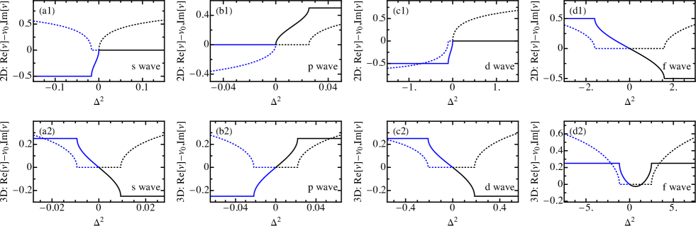
Figure 1: (Color online): $\nu$ of the first four partial wave cases for 2D (a1-d1) and 3D (a2-d2). The black and blue lines are for replusive and attractive potentials, respectively. The real part and imaginary part of $\nu$ are corresponding to solid lines and dashed lines.

As shown above, one key step in constructing the exact solutions is obtaining $\nu$ under given energy $\epsilon$ and partial wave $\overline{l}$ by searching the root of the characteristic function $\Lambda_{\overline{l}}(\nu,\varepsilon_{s})$ in Eq. (20). On the complex plane, although there are infinite branches of solutions in $\nu$, the physical solution is unique and corresponds to the one that approaches $\nu_{0}$ as $\epsilon\rightarrow 0$ and changes continuously as $|\epsilon|$ increases Gao (1998); Jie and Qi (2016) and this root becomes complex beyond a critical scaled energy $\Delta_{c}$ being shown in Table 2 for the first four partial waves in 2D and 3D.

In Fig. 1, we show the energy dependence of $\nu$ for the first four partial waves of 2D (a1-d1) and 3D (a2-d2). For 3D (a2-d2), the low critical energy exists for each partial wave, i.e., $\nu$ becomes complex beyond the critical energies $|\Delta_{c}^{2}|$. While for 2D, $\nu$ can be purely imaginary for the first three partial waves. For arbitrary partial waves $l$ and $m$, Re$[\nu]$ goes to a plateaus when $|\Delta^{2}|$ beyond the critical energies $|\Delta_{c}^{2}|$.

Table 2: Critical scaled energy $\Delta^{2}_{c}=(\overline{\epsilon}_{c}L^{2}/8)^{2}$ for the first four partial wave. $\Delta^{2}\leq 0$ and $\Delta^{2}\geq 0$ are corresponding to repulsive and attractive potential cases, respectively.

Partial Wave	Two dimension		Three dimension
	Repulsive	Attractive	Repulsive	Attractive
$s$	-0.0169	0	-0.00933	0.00932
$p$	0	0.0253	-0.0218	0.0217
$d$	-0.103	0	-0.209	0.185
$f$	-1.60	1.59	-1.17	2.50

Those general behaviors can be numerically obtained. However, we also can extract analytic information at the low scattering energy limit by performing the small $\Delta$ expansion to $\Lambda_{\overline{l}}(\nu,\Delta^{2})$. In practice, we can analytically obtain the root of the characteristic function in Eq. (20),

$$\nu=\nu_{0}-\frac{3\Delta^{2}}{\nu_{0}\left(1-\nu_{0}^{2}\right)\left(1-4\nu_{0}^{2}\right)}$$

$$-\frac{9\left[8-7\nu_{0}^{2}\left(21-45\nu_{0}^{2}+20\nu_{0}^{4}\right)\right]\Delta^{4}}{4\nu_{0}^{3}\left(4-\nu_{0}^{2}\right)\left(1-\nu_{0}^{2}\right)^{3}\left(1-4\nu_{0}^{2}\right)^{3}}+O\left(\Delta^{5}\right),$$ (53)

which takes $\nu_{0}$ when the scaled energy $\Delta$ vanishes and it diverges when $\nu_{0}=0,1/2,1,2$ which are corresponding to the angular moments $m=0,1,2,4$ in 2D. The low energy expansion expressions of those specific cases are given as

$$\nu_{m=0} = \frac{i}{16}\sqrt{\frac{3}{2}}\left(32-315\Delta^{2}\right)\Delta+O\left(\Delta^{5}\right),$$ (54)

$$\nu_{m=1} = \frac{1}{2}+\left(2+\frac{119\Delta^{2}}{9}\right)\Delta+O\left(\Delta^{5}\right),$$ (55)

$$\nu_{m=2} = 1+\left(i-\frac{\Delta}{48}\right)\Delta+O\left(\Delta^{3}\right),$$ (56)

$$\nu_{m=3} = \frac{3}{2}-\left(\frac{1}{5}-\frac{1291\Delta^{2}}{10500}\right)\Delta^{2}+O\left(\Delta^{5}\right),$$ (57)

$$\nu_{m=4} = 2+\left[\frac{3-i}{120}+\left(\frac{377}{432000}+\frac{71i}{27000}\right)\Delta^{2}\right]\Delta^{2}$$ (58)

$$+O\left(\Delta^{5}\right).$$

III Quantum defect theory of the Van der Waals potentials in quasi-2D and 3D

One classical example to understanding the quantum defect theory is the energy spectrum of hydrogen atom and alkali atoms Seaton (1983). For hydrogen atom, there is only one electron moving around the nucleus, and the energy spectrum is simply proportional to $1/n^{2}$, with $n$ being the principle quantum number. While for the alkali atoms, in addition to the outermost electron, there are still inner-shell electrons which will provide the penetration effect and screening effect when the outermost electron moving around the nucleus. Therefore, one need to introduce a parameter $\Delta$ for the energy spectrum of alkali atoms to describe those short range effects and then the modified energy spectrum could be simply proportional to $1/(n-\Delta)^{2}$ compared to the one of the hydrogen atom. The introduced parameter $\Delta$ contains the information of the short range potential of the outermost electron and usually be called as quantum defect parameter.

For ultracold and dilute molecular gases, the average distance between two molecule is much larger than the Van der waals length and then we usually can model the two-body interaction by the contact interaction associated with the scattering length which contains the information of short range potentials Chin et al. (2010). Either when one wants to have more accurate two-body scattering properties or when the molecular gases are not enough cold and dilute, we need to consider the Van der waals type shorter range potential, which can be induced from two polar molecules tuning by electric fields Matsuda et al. (2020); Li et al. (2021). More specific, we consider two ⁴⁰K⁸⁷Rb molecules prepared in the $|N,m_{N}\rangle=|1,0\rangle$ state, where $N$ is the rotational angular momentum and $m_{N}$ is its projection along the axis of electric field ${\bf E}$. Starting from this two-molecular state $|1,0\rangle\otimes|1,0\rangle$ at weak electric field ${\bf E}$, we then increase the strength of electric field $|{\bf E}|$ to across two crossing energy points, where the two molecular states are $|0,0\rangle\otimes|2,\pm 1\rangle$ and $|0,0\rangle\otimes|2,0\rangle$, respectively. Near the crossing points, the two molecular states are coupled by the dipole interaction which weakly opens the energy gap via a second order perturbation process. Thus the effective attractive (repulsive) Van der Waals barrier in the energy curve of these two molecules associated with state $|0,0\rangle\otimes|2,\pm 1\rangle$ ($|0,0\rangle\otimes|2,0\rangle$) emerges. This new technique for inducing the effective Van der Waals potentials both be realized in quasi-2D Matsuda et al. (2020) and 3D Li et al. (2021). Next, we will construct the quantum defect theories for these systems.

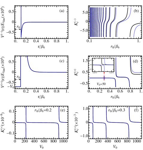
Figure 2: (Color online): Quantum defect parameter for two potential configurations $V^{(-)}$ (a-b) and $V^{(+)}$ (c-f). The black solid lines are for 3D and the dashed blue lines are for 2D. In (a-b), all cases are $s$ wave. In (c-f), $s$ wave and $p$ wave are picked up for 3D and 2D cases, respectively.

III.1 Quantum defect parameter $K_{c}$

In Eqs. (4-7), we have the pair of linearly independent specific solutions. Usually, the general solutions are obtained by linearly combining those specific solutions which can be written as

$$u_{\overline{\epsilon}\overline{l}}^{\pm}(r)=A\left[u_{\overline{\epsilon}\overline{l}}^{\pm 1}(r)-K_{c}^{(\pm)}u_{\overline{\epsilon}\overline{l}}^{\pm 2}(r)\right],$$ (59)

where the relative superposition coefficient $K_{c}^{(\pm)}$ is the quantum defect parameter which contains the short range information of the systems. At positive scattering energy, the phase shift can be deduced by the asymptotic behaviors of $u_{\overline{\epsilon}\overline{l}}^{\pm 1}(r)$ and $u_{\overline{\epsilon}\overline{l}}^{\pm 2}(r)$ in Eqs. (II.2-II.2),

$$\text{3D}:~{}\tan\delta_{l}^{\pm} = \frac{K_{c}^{(\pm)}Z_{22}^{\pm}-Z_{12}^{\pm}}{Z_{11}^{\pm}-K_{c}^{(\pm)}Z_{21}^{\pm}},$$ (60)

$$\text{2D}:~{}\tan\delta_{m}^{\pm} = \frac{K_{c}^{(\pm)}(Z_{21}^{\pm}+Z_{22}^{\pm})-(Z_{11}^{\pm}+Z_{12}^{\pm})}{(Z_{11}^{\pm}-Z_{12}^{\pm})-K_{c}^{(\pm)}(Z_{21}^{\pm}-Z_{22}^{\pm})}.~{}~{}$$ (61)

The scattering sections are related to the phase shifts as following,

$$\text{3D}:~{}\sigma_{l}^{\pm} = 4\pi(2l+1)\frac{\sin^{2}\delta_{l}^{\pm}}{k^{2}},$$ (62)

$$\text{2D}:~{}\sigma_{m}^{\pm} = 4\frac{\sin^{2}\delta_{m}^{\pm}}{k}.~{}~{}$$ (63)

Since the physical bound states must exponentially decay at large $r$ and then the binding energy $E_{b}$ can be determined by requiring the coefficient of $e^{\kappa r}$ terms of $u_{\overline{\epsilon}\overline{l}}^{\pm}(r)$ in Eqs. (32-33) to be vanished. This straightforwardly leads to the equation for the binding energy $E_{b}$,

$$W_{11}^{\pm}-K_{c}^{(\pm)}W_{21}^{\pm}=0,$$ (64)

and then we can define one function to characterize the bound states,

$$\chi^{\pm}_{\widetilde{l}}(E_{b})=K_{c}^{(\pm)}=W_{11}^{\pm}/W_{21}^{\pm}.$$ (65)

Therefore, either for obtaining the phase shift in Eqs. (60-61) or for extracting the energies of bound states from Eq. (65), the quantum defect parameter $K_{c}^{(\pm)}$ needs to be given firstly. Furthermore, according to the asymptotic behaviors in the short range $r\ll\beta_{6}$, the partial wave and energy are insensitive to the wave functions [shown in Eqs. (22-25)] and the quantum defect parameter $K_{c}^{(\pm)}$. To illustrate this, we divid the overall potentials into long-range tails and short-range part by the boundary $r=r_{0}$. The long-range tails are the Van der Waals potentials $\pm C_{6}/r^{6}$ and we construct a square potential with finite depth and a square barrier potential with infinity height as short-range model potentials for repulsive and attractive long-rang potentials as shown in Eqs. (III.1-III.1) and in Fig. 2(a,c), respectively.

$$V^{(+)} = -V_{0}\theta(r_{0}-r)E_{\text{Van}}+\theta(r-r_{0})\frac{\hbar^{2}}{2\mu}\left[\frac{\overline{l}(\overline{l}+1)}{r^{2}}+\frac{\beta_{6}^{4}}{r^{6}}\right],$$

$$V^{(-)} = +\infty\theta(r_{0}-r)E_{\text{Van}}+\theta(r-r_{0})\frac{\hbar^{2}}{2\mu}\left[\frac{\overline{l}(\overline{l}+1)}{r^{2}}-\frac{\beta_{6}^{4}}{r^{6}}\right],$$

where $E_{\text{Van}}=\hbar^{2}/(2\mu\beta_{6}^{2})$ is the characteristic energy scale associated with the Van der Waals length $\beta_{6}$. In additional, through the boundary conditions, we can analytically obtain the expressions for the quantum defect parameter $K_{c}^{(\pm)}$ with zero energy as

$$K^{(+)}_{c} = i^{2\nu_{0}+1}\frac{2r^{3}\sqrt{V_{0}}H_{\nu_{0}}^{(1)}\left(\frac{L^{2}}{r^{2}}\right)\cos\left(\frac{r\sqrt{V_{0}}}{\beta_{6}}\right)+\beta_{6}\left[4L^{2}H_{\nu_{0}-1}^{(1)}\left(\frac{L^{2}}{r^{2}}\right)-\left(4\nu_{0}+1\right)r^{2}H_{\nu_{0}}^{(1)}\left(\frac{L^{2}}{r^{2}}\right)\right]\sin\left(\frac{r\sqrt{V_{0}}}{\beta_{6}}\right)}{4r^{3}\sqrt{V_{0}}J_{\nu_{0}}\left(\frac{L^{2}}{r^{2}}\right)\cos\left(\frac{r\sqrt{V_{0}}}{\beta_{6}}\right)-2\beta_{6}\left[\left(4\nu_{0}+1\right)r^{2}J_{\nu_{0}}\left(\frac{L^{2}}{r^{2}}\right)-4L^{2}J_{\nu_{0}-1}\left(\frac{L^{2}}{r^{2}}\right)\right]\sin\left(\frac{r\sqrt{V_{0}}}{\beta_{6}}\right)},$$ (68)

and

$$K^{(-)}_{c} = \frac{J_{\nu_{0}}\left(\frac{L^{2}}{r_{0}^{2}}\right)}{Y_{\nu_{0}}\left(\frac{L^{2}}{r_{0}^{2}}\right)}.$$ (69)

In Fig. 2, we show the behaviours of $K_{c}^{(\pm)}$ when varying the short-range parameters. The black solid lines are for 3D and the dashed blue lines are for 2D. For the attractive cases as shown in Fig. 2(b), the number density of the resonances are increasing rapidly when the range $r_{0}$ decreases to zero. In contrast, for the repulsive cases as shown in Fig. 2(d-f), the number density of the resonances are much more dilute and extremely narrow compared to that of the attractive cases and $K_{c}^{(+)}$ approaches to zero for most regions. Interestingly, there even doesn’t exist significant resonance when the range $r_{0}$ goes to zero given the square potential depth $V_{0}$. This behavior is mainly due to the existence of a large repulsive barrier which makes the wave function almost unaffected by the short range attractive part of the potential. Therefore, we will only consider the scattering behaviour in the pure repulsive limit ($r_{0}\rightarrow 0$), i.e., $K_{c}^{(+)}=0$, while for the attractive case, we will investigate both the scattering and bound state properties across a shape resonance where $K_{c}^{(-)}$ can be tuned from $+\infty$ to $-\infty$.

III.2 Scattering property and bound state

Figure 3: (Color online): Phase shifts and scattering sections of the first four partial waves for 2D (a-b) and 3D (c-d) for the purely repulsive potentials. The black solid lines, red dashed lines, blue dotted lines, and green dotted dashed lines are corresponding to $s$ wave, $p$ wave, $d$ wave, and $f$ wave, respectively. The thin gray lines are the total scattering sections of the first four waves. The dotted symbols are from the low energy expansions of scattering phase shifts in Eqs. (72-79). The low energy expansions of scattering cross sections are tediously to write down. The scaled moment is defined as $k_{s}=k\beta_{6}$.

For the pure repulsive cases, we only consider the scattering phase shift by taking $K_{c}^{(+)}=0$ in Eqs. (60-61) and then we have

$$\text{3D}:~{}\tan\delta_{l}^{+} = -\frac{Z_{12}^{\pm}}{Z_{11}^{\pm}},$$ (70)

$$\text{2D}:~{}\tan\delta_{m}^{\pm} = -\frac{Z_{11}^{\pm}+Z_{12}^{\pm}}{Z_{11}^{\pm}-Z_{12}^{\pm}}.~{}~{}$$ (71)

In Fig. 3, we show the phase shifts and scattering sections of the first four partial waves. The phase shifts starts from zero as the energy increasing and will induce a deep in the scattering section when it crosses $n\pi$ with integer $n$ (see the black curve in (b)). For the scattering sections, the $s$ wave dominates in the low energy regime and then higher partial waves take place $s$ wave in the high energy regime. In the limit $k\rightarrow 0$, the scattering section converges to $\pi\left[\Gamma\left(\frac{3}{4}\right)/\Gamma\left(\frac{5}{4}\right)\right]^{2}$ for 3D and is divergent for 2D. Furthermore, we can analytically expand the phase shifts in the low energy regime as following,

$$\tan\delta_{m=0}^{+} = \frac{\pi}{2\ln k_{s}+3\gamma-4\ln 2},$$ (72)

$$\tan\delta_{m=1}^{+} = \frac{\pi k_{s}^{2}\left[(19-36\gamma+24\ln(\frac{2}{k_{s}}))k_{s}^{2}-48\right]}{384},$$ (73)

$$\tan\delta_{m=2}^{+} = \frac{\pi k_{s}^{4}\left(24\ln k_{s}+36\gamma-11-48\ln 2\right)}{3072},$$ (74)

$$\tan\delta_{m=3}^{+} = -\frac{\pi k_{s}^{4}}{1280},$$ (75)

for 2D, and

$$\tan\delta_{l=0}^{+} = -\left[\frac{2\Gamma\left(\frac{3}{4}\right)}{\Gamma\left(\frac{1}{4}\right)}+\frac{\pi k_{s}^{3}}{15}\right]k_{s},$$ (76)

$$\tan\delta_{l=1}^{+} = -\left[\frac{\Gamma\left(\frac{1}{4}\right)}{24\Gamma\left(\frac{7}{4}\right)}-\frac{\pi k_{s}}{35}\right]k_{s}^{3},$$ (77)

$$\tan\delta_{l=2}^{+} = -\frac{\pi}{315}k_{s}^{4},$$ (78)

$$\tan\delta_{l=3}^{+} = -\frac{\pi}{3465}k_{s}^{4},$$ (79)

for 3D with $\gamma$ being the Euler’s constant .We show the agreements in Fig. 3 when compare those approximated analytical results (symbols) to the exact numerical results (lines).

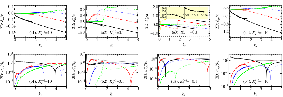
Figure 4: (Color online): Phase shifts and scattering sections of the first four partial waves for 2D (a1-b4) and 3D (c1-d4) for the potentials with attractive Van der Waals tails. The black solid lines, red dashed lines, blue dotted lines, and green dotted dashed lines are corresponding to $s$ wave, $p$ wave, $d$ wave, and $f$ wave, respectively. The thin gray lines are the total scattering sections of the first four waves. The dotted symbols are from the low energy expansions in Eqs. (80-83). The low energy expansions of scattering cross sections are tediously to write down. The scaled moment is defined as $k_{s}=k\beta_{6}$.

For the attractive cases in 2D, we consider both scattering properties and bound states of the first four partial waves as shown in Figs. 4 and 5. We pick up four sets of quantum defect parameter across the positive side to the negative side by taking $K_{c}^{(-)}=10,0.1,-0.1,10$ in Fig. 4. For the s-wave, the scattering sections are divergent when $k\rightarrow 0$, and there is one extremely narrow phase jumping in the case $K_{c}^{(-)}=-0.1$ with the details showing in the inset of Fig. 4(a3). Some other phase jumping are shown in the higher partial waves in Fig. 4(a2), which corresponding to the local maximals in the scattering sections in Fig. 4(b2). The low energy analytical expansions for the scattering phase shifts are in following,

$$\tan\delta_{m=0}^{-} = \frac{2\pi K_{c}^{(-)}}{A}-\frac{\pi^{2}\left(K_{c}^{(-)}{}^{2}+1\right)k_{s}^{2}}{2A^{2}},$$ (80)

$$\tan\delta_{m=1}^{-} = \frac{\pi k_{s}^{2}}{8K_{c}^{(-)}},$$ (81)

$$\tan\delta_{m=2}^{-} = \frac{\pi(7K_{c}^{(-)}-4A)k_{s}^{4}}{2048K_{c}^{(-)}},$$ (82)

$$\tan\delta_{m=3}^{-} = \frac{\pi k_{s}^{4}}{1280},$$ (83)

where $A=4K_{c}^{(-)}\ln k_{s}+6\gamma K_{c}^{(-)}-8K_{c}^{(-)}\ln 2-\pi$.

The energy of bound states are determined by Eq. (65), which is characterized by the asymptotic behaviors describing long range properties and the quantum defect parameter $K_{c}^{(-)}$ encoding the short range information. In Fig. 5, we show the energy of bound states for the first four partial waves varying with the quantum defect parameter $K_{c}^{(-)}$, where the dots are from exact solutions and the blue solid lines are from the low energy expansions below,

$$\chi_{m=0}^{-} = \frac{\pi}{2B}+\frac{\left(4B^{2}+\pi^{2}\right)k_{s}^{2}}{16B^{2}},$$ (84)

$$\chi_{m=1}^{-} = \frac{2B-3+4\ln 2}{16}\left(1+\frac{\pi k_{s}^{2}}{8}\right)k_{s}^{2}-\frac{\pi k_{s}^{4}}{768},$$ (85)

$$\chi_{m=2}^{-} = -\frac{k_{s}^{2}}{12}+\frac{\pi(7-8B)k_{s}^{4}}{4096},$$ (86)

$$\chi_{m=3}^{-} = -\frac{k_{s}^{2}}{32}+\frac{\pi k_{s}^{4}}{2560}$$ (87)

where $B=2\ln k_{s}+3\gamma-4\ln 2$.

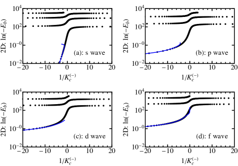
Figure 5: (Color online): Bound states of the first four partial waves in 2D for the potentials with attractive tails. The black dotted symbols are from exact solutions and the blue solid lines are from the low energy expansions in Eqs. (84-87)

From Fig. 5, we find the shallow bound state only exists in the $s$ wave when the quantum defect parameter $K_{c}^{(-)}$ goes to infinity and the deep bound states are ordering from all the partial wave branches. All the numerical results (dotted points) agrees well with the analytical expressions (lines) in the low energy limitation.

IV Conclusions and discussions

In this work, we firstly provide the exact solutions for the 2D and 3D Schrödinger equations with isotropic Van der Waals interactions ($\pm 1/r^{6}$) by the generalized Neumann expansion and then give the detailed analysis of the asymptotic behaviors. Base on these exact solutions and asymptotic behaviors, we construct quantum defect theories for the two-body problems with Van der Waals type potential tails both in quasi-2D and 3D systems. The scattering properties and two-body bound states are investigated both by the exact numerical calculations and low energy expansion formulas. All these results could be applied to the recently experimental realized long-lived polar molecular gases in quasi-2D and 3D Matsuda et al. (2020); Li et al. (2021). Furthermore, our results could be useful to future many-body studies involving the long range Van der Waals interactions ($\pm 1/r^{6}$) and will show the insights to the systems with other interesting long range interactions.

References

• (1) N. Defenu, T. Donner, T. Macrì, G. Pagano, S. Ruffo,  and A. Trombettoni, “Long-range interacting quantum systems,” arXiv:2109.01063 .
• Schneider et al. (2012) C. Schneider, D. Porras,  and T. Schaetz, “Experimental quantum simulations of many-body physics with trapped ions,” Reports on Progress in Physics 75, 024401 (2012).
• Ritsch et al. (2013) H. Ritsch, P. Domokos, F. Brennecke,  and T. Esslinger, “Cold atoms in cavity-generated dynamical optical potentials,” Rev. Mod. Phys. 85, 553–601 (2013).
• Schauß et al. (2012) P. Schauß, M. Cheneau, M. Endres, T. Fukuhara, S. Hild, A. Omran, T. Pohl, C. Gross, S. Kuhr,  and I. Bloch, “Observation of spatially ordered structures in a two-dimensional Rydberg gas,” Nature 491, 87–91 (2012).
• Ni et al. (2008) K-K Ni, S. Ospelkaus, M. De Miranda, A. Pe’Er, B. Neyenhuis, J. Zirbel, S. Kotochigova, P. S. Julienne, D. S. Jin,  and J. Ye, “A high phase-space-density gas of polar molecules,” science 322, 231–235 (2008).
• Jin and Ye (2012) D. S. Jin and J. Ye, “Introduction to ultracold molecules: new frontiers in quantum and chemical physics,” Chemical reviews 112, 4801–4802 (2012).
• Liu and Ni (2021) Y. Liu and K-K Ni, “Bimolecular chemistry in the ultracold regime,” Annual review of physical chemistry 73 (2021).
• Ospelkaus et al. (2010) S. Ospelkaus, K-K Ni, D. Wang, M. De Miranda, B. Neyenhuis, G. Quéméner, P. S. Julienne, J. Bohn, D. S. Jin,  and J. Ye, “Quantum-state controlled chemical reactions of ultracold potassium-rubidium molecules,” Science 327, 853–857 (2010).
• Ye et al. (2018) X. Ye, M. Guo, M. González-Martínez, G. Quéméner,  and D. Wang, “Collisions of ultracold 23Na87Rb molecules with controlled chemical reactivities,” Science advances 4, eaaq0083 (2018).
• Hu et al. (2019) M-G Hu, Y. Liu, D. Grimes, Y-W Lin, A. Gheorghe, R. Vexiau, N. Bouloufa-Maafa, O. Dulieu, T. Rosenband,  and K-K Ni, “Direct observation of bimolecular reactions of ultracold KRb molecules,” Science 366, 1111–1115 (2019).
• Matsuda et al. (2020) K. Matsuda, L. De Marco, J-R Li, W. Tobias, G. Valtolina, G. Quéméner,  and J. Ye, “Resonant collisional shielding of reactive molecules using electric fields,” Science 370, 1324–1327 (2020).
• Li et al. (2021) J-R Li, W. Tobias, K. Matsuda, C. Miller, G. Valtolina, L. De Marco, R. Wang, L. Lassablière, G. Quéméner, J. Bohn,  and J. Ye, “Tuning of dipolar interactions and evaporative cooling in a three-dimensional molecular quantum gas,” Nature Physics 17, 1144–1148 (2021).
• Gao (1998) Bo Gao, “ Solutions of the Schrödinger equation for an attractive $1/r^{6}$ potential,” Phys. Rev. A 58, 1728–1734 (1998).
• Jie and Qi (2016) Jianwen Jie and Ran Qi, “Exact two-body solutions and quantum defect theory of two-dimensional dipolar quantum gas,” Journal of Physics B: Atomic, Molecular and Optical Physics 49, 194003 (2016).
• Gao (1999) Bo Gao, “Repulsive ${1/r}^{3}$ interaction,” Phys. Rev. A 59, 2778–2786 (1999).
• Greene et al. (1979) C. Greene, U. Fano,  and G. Strinati, “General form of the quantum-defect theory,” Phys. Rev. A 19, 1485–1509 (1979).
• Greene et al. (1982) Chris H. Greene, A. R. P. Rau,  and U. Fano, “General form of the quantum-defect theory. II,” Phys. Rev. A 26, 2441–2459 (1982).
• Mies (1984) Frederick H. Mies, “A multichannel quantum defect analysis of diatomic predissociation and inelastic atomic scattering,” The Journal of Chemical Physics 80, 2514–2525 (1984).
• Gao et al. (2005) Bo Gao, Eite Tiesinga, Carl J. Williams,  and Paul S. Julienne, “Multichannel quantum-defect theory for slow atomic collisions,” Phys. Rev. A 72, 042719 (2005).
• Gao (2008) Bo Gao, “General form of the quantum-defect theory for $-1/{r}^{\alpha}$ type of potentials with $\alpha>2$,” Phys. Rev. A 78, 012702 (2008).
• Gao (2009) Bo Gao, “Analytic description of atomic interaction at ultracold temperatures: The case of a single channel,” Phys. Rev. A 80, 012702 (2009).
• Cavagnero (1994) M. J. Cavagnero, “Secular perturbation theory of long-range interactions,” Phys. Rev. A 50, 2841–2846 (1994).
• Abramowitz and Stegun (1964) Milton Abramowitz and Irene A Stegun, Handbook of mathematical functions with formulas, graphs, and mathematical tables, Vol. 55 (US Government printing office, 1964).
• Watson (1995) George Neville Watson, A treatise on the theory of Bessel functions (Cambridge university press, 1995).
• Seaton (1983) MJ Seaton, “Quantum defect theory,” Reports on Progress in Physics 46, 167 (1983).
• Chin et al. (2010) Cheng Chin, Rudolf Grimm, Paul Julienne,  and Eite Tiesinga, “Feshbach resonances in ultracold gases,” Rev. Mod. Phys. 82, 1225–1286 (2010).