secReference

Zeptonewton force sensing with squeezed quadratic optomechanics

Cavity optomechanical (COM) sensors, as powerful tools for measuring ultraweak forces or searching for dark matter, have been implemented to date mainly using linear COM couplings. Here, quantum force sensing is explored by using a quadratic COM system which is free of bistability and allows accurate measurement of mechanical energy. We find that this system can be optimized to achieve a force sensitivity $7$ orders of magnitude higher than any conventional linear COM sensor, with experimentally accessible parameters. Further integrating a quadratic COM system with a squeezing medium can lead to another $3$ orders enhancement, well below the standard quantum limit and reaching the zeptonewton level. This opens new prospects of making and using quantum nonlinear COM sensors in fundamental physics experiments and in a wide range of applications requiring extreme sensitivity.

Rapid advances have been witnessed in recent years in fabricating high resolution and noninvasive chip-scale quantum sensors Clerk et al. (2010); Pirandola et al. (2018), enabling both tests of fundamental physics Vermeulen et al. (2021); Westphal et al. (2021) and diverse applications Forstner et al. (2012); Krause et al. (2012). Such sensors are implemented using, e.g., microwave circuits Clark et al. (2016); Wollman et al. (2015); Pirkkalainen et al. (2015); Suh et al. (2014), cold ions or atoms Burd et al. (2019); Møller et al. (2017) and mechanical resonators Rossi et al. (2018); Wilson et al. (2015). In particular, COM sensors exploiting coherent light-motion coupling have led to the milestone achievement of gravitational-wave observations Whittle et al. (2021); Yu et al. (2020); Aggarwal et al. (2020); Cripe et al. (2019); Yap et al. (2020). For all quantum sensors, the first step is to reduce thermal noise down to the level of zero-point fluctuations, reaching the standard quantum limit (SQL) with an optimal balance of the measurement and its unwanted backaction Braginsky and Khalili (1996). Then, quantum resources are utilized to go beyond the SQL, as done in state-of-the-art COM experiments Ockeloen-Korppi et al. (2018, 2017); Sudhir et al. (2017); Purdy et al. (2017); de Lépinay et al. (2021); Shomroni et al. (2019a, b); Ockeloen-Korppi et al. (2016); Lecocq et al. (2015); Safavi-Naeini et al. (2013). In a very recent example Yu et al. (2020), a sub-SQL measurement of displacement was demonstrated by injecting squeezed light into the LIGO interferometer with mirrors each weighing $40\text{\,}\mathrm{kg}$. As far as we know, COM sensors to date have relied on the lowest-order COM coupling, featuring a linear relationship between the optical cavity detuning and the mechanical displacement Sankey et al. (2010).

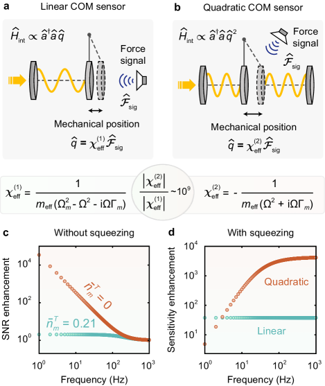
Figure 1: Comparisons of linear and quadratic COM sensing. a-b The force signal, modulating the oscillations of the end mirror or the membrane in the middle of the cavity, can be detected through the optical output of the COM system. c Enhancement of signal-to-noise ratio (SNR) of the quadratic COM sensor compared with the linear COM sensor. d When including an intracavity squeezing medium, sensitivity can be further enhanced for the quadratic or linear COM sensor.

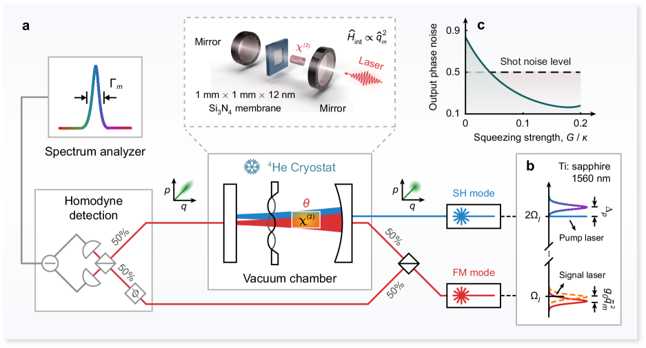
Figure 2: Quantum force sensing with a quadratic COM system. a A thin dielectric membrane, placed at a node (or antinode) of the standing waves of a Fabry–Pérot cavity, is coupled quadratically with the cavity field, allowing for quantum non-demolition readout of the membrane’s phonon numbers Thompson et al. (2008); Sankey et al. (2010). b The signal laser at wavelength $1560\text{\,}\mathrm{nm}$ pumps the fundamental (FM) mode at its parametric resonance Bruch et al. (2019). The $\chi^{(2)}$ nonlinear medium, driven by a pump laser, creates a nonlinear coupling of the FM mode and the second-harmonic (SH) mode Bruch et al. (2019). The mechanical vibrations imprinted on the variational quadrature of the signal laser can then be detected in a homodyne device Brawley et al. (2016). c The output phase noise as a function of the squeezing strength. The background noise inside the squeezing medium can be suppressed below the shot noise limit Peano et al. (2015).

Here we study a squeezed COM sensor based on quadratic optomechanics and show a giant enhancement in the sensitivity of force measurements. We note that quadratic COM systems have been experimentally demonstrated by using e.g., levitated nanoparticles Bullier et al. (2021), photonic crystals Paraïso et al. (2015), ultracold atoms Purdy et al. (2010), and membrane-in-the-middle (MIM) cavities Thompson et al. (2008); Sankey et al. (2010). In contrast to linear COM devices, quadratic COM systems are free of bistability Sankey et al. (2010), allow accurate measurements of mechanical energy Thompson et al. (2008); Lee et al. (2015), and have improved signal-to-noise ratio (SNR) in measurements due to their counterintuitive ability of amplifying signal imprinted on the quadratures Brawley et al. (2016); Leijssen et al. (2017). These features of quadratic COM systems, however, have not been fully explored for sensing applications. Here, we show that in comparison with conventional COM sensors Wilson et al. (2015); Sudhir et al. (2017), a $7$ orders of magnitude enhancement in sensitivity can be achieved for a quadratic COM sensor. Also, by exploiting intracavity squeezing Bruch et al. (2019); Peano et al. (2015), the force sensitivity can be further improved by $3$ orders of magnitude, well below the SQL, reaching zeptonewton level at cryogenic temperatures.

The advantages of a quadratic COM sensor, compared with conventional COM sensors, are twofold (see Fig. 1a-b): (i) its response to weak force signals is more sensitive than that of the linear COM system, due to its stronger effective mechanical susceptibility (see the Methods), which can lead to many orders improvement in SNR (Fig. 1c); (ii) when an intracavity squeezing medium is incorporated, the enhancement in force sensitivity in a quadratic COM sensor becomes much larger than that in a linear COM sensor (Fig. 1d). In view of rapid advances of COM experiments, we believe that such a quadratic COM sensor can be realized not only with an MIM cavity, but also by using superconducting circuits Ma et al. (2021), levitated particles Bullier et al. (2021); Magrini et al. (2021), or trapped ions Gilmore et al. (2021). Our work sheds new light on squeezed COM and its applications in a wide range of fields including nonlinear frequency comb Bruch et al. (2021), non-demolition measurements of dark matter or quantum wave function Manley et al. (2021); Forstner et al. (2020), and noninvasive biological imaging or quantum illumination Taylor et al. (2013); Casacio et al. (2021); Basiri-Esfahani et al. (2019); Gil-Santos et al. (2020); Barzanjeh et al. (2015).

Results

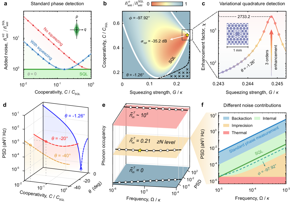
Figure 3: The added noise and the power spectral density (PSD). a The added noise, with or without squeezing, for standard phase detection. b-c The added noise for variational quadrature detection. The white solid line and the black dashed line denote the SQL and the mechanical response of $\mathcal{R}_{m}^{\phi}\quantity[\Omega]=1$, respectively. The input signal is suppressed in the marked region (‘$\times$’) but amplified in other regions. c The enhancement factor versus the squeezing strength. The inset shows the structure of the soft-clamped mechanical resonator (Si3N4 in blue, holes in white) Galinskiy et al. (2020). d The PSD as a function of the cooperativity and the squeezing phase. The solid or dashed curves denote the results in the stable or unstable region, respectively, where the circles give the minimum PSD in the stable region. e-f The PSD for different phonon occupations when the cavity coupling parameter is $\eta_{c}=0.97$ (ref. Rossi et al. (2018)). The yellow stars in (b) and (e) denote the highest force sensitivity (i.e., zeptonewton scale) at mean phonon occupations of $0.21$ (ref. Galinskiy et al. (2020)). The curves in (f) indicate the total spectra under the standard phase detection (blue) and the fixed ‘non-standard’ quadrature detection (light green). The green line denotes the SQL.

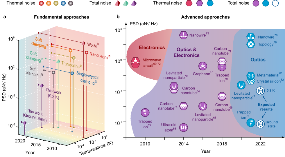
Figure 4: Quantum force sensing and its development. a PSD reported for conventional COM sensors with silicon nitride membranes Catalini et al. (2020); Hälg et al. (2021); Gavartin et al. (2012); Mason et al. (2019); Reinhardt et al. (2016); Tsaturyan et al. (2017); Schliesser et al. (2009); Tao et al. (2014). In comparison with current experiments, our proposal achieves higher force sensitivity at ground state Galinskiy et al. (2020) or hundreds of millikelvin temperatures Schliesser et al. (2009). WGM: whispering-gallery-mode microresonators. b The evolution of ultrasensitive force measurements Beccari et al. (a, b); Biercuk et al. (2010); Moser et al. (2013); Rodenburg et al. (2016); Schreppler et al. (2014); Weber et al. (2016); De Bonis et al. (2018); Hertzberg et al. (2010); Gieseler et al. (2013); Dadras et al. ; Teufel et al. (2009); Gloppe et al. (2014); Moser et al. (2014); Liu et al. (2021); Fogliano et al. (2021a); Tavernarakis et al. (2018); Høj et al. (2021); Blūms et al. (2018). When the hierarchical metamaterials are employed in the MIM cavity Beccari et al. (a), the total force sensitivity for our scheme is expected to reach $\quantity($9.9\text{\,}\mathrm{zN}$)^{2}$\mathrm{/}\mathrm{Hz}$$ at the temperature of $0.2\text{\,}\mathrm{K}$ (ref. Schliesser et al. (2009)), and can be improved to $\quantity($70.5\text{\,}\mathrm{yN}$)^{2}$\mathrm{/}\mathrm{Hz}$$ near the motional ground state Galinskiy et al. (2020), approaching the precisions of ultracold atoms and ions Schreppler et al. (2014); Liu et al. (2021).

Squeezed quadratic optomechanical system

We consider an MIM cavity integrated with an intracavity squeezing medium Sankey et al. (2010); Bruch et al. (2019), as illustrated in Fig. 2. The cavity field supports a fundamental (FM) mode at frequency $\Omega_{l}$, denoted by the annihilation operator $\hat{a}$, which has the typical decay rate $\kappa/2\pi=$2.75\text{\,}\mathrm{MHz}$$ (ref. Galinskiy et al. (2020)) and the quality factor $Q=$1.1\text{\times}{10}^{7}$$ (ref. Galinskiy et al. (2020)). The cavity coupling parameter is defined as $\eta_{c}=\kappa_{\mathrm{ex}}/(\kappa_{0}+\kappa_{\mathrm{ex}})$, where $\kappa_{0}$ and $\kappa_{\mathrm{ex}}$ denote the intrinsic and external decay rate, respectively. The intracavity $\chi^{(2)}$ crystal, driven by the pump laser at frequency $2\Omega_{l}$, generates the nonlinear coupling of the FM mode and the second-harmonic (SH) mode Qin et al. (2021). Both optical modes can be coupled quadratically Thompson et al. (2008); Sankey et al. (2010) to the mechanical mode at frequency $\Omega_{m}/2\pi=$1\text{\,}\mathrm{MHz}$$ (ref. Galinskiy et al. (2020)), denoted by the dimensionless annihilation operators $\hat{q}_{m}$ and $\hat{p}_{m}$, with the mechanical decay rate $\Gamma_{m}$, the effective mass $m_{\mathrm{eff}}=$1\text{\,}\mathrm{ng}$$ (ref. Galinskiy et al. (2020)), and the mechanical quality factor $Q_{m}=$5\text{\times}{10}^{8}$$ (ref. Galinskiy et al. (2020)). For a strong pump field, the fluctuations of the SH mode can be neglected and therefore the Hamiltonian of the system can be written at the simplest level as Thompson et al. (2008); Peano et al. (2015)

$$\hat{H} =\hbar\Delta_{c}\hat{a}^{\dagger}\hat{a}+\frac{\hbar}{2}\Omega_{m}\quantity(\hat{q}_{m}^{2}+\hat{p}_{m}^{2})-\hbar g_{0}\hat{a}^{\dagger}\hat{a}\hat{q}_{m}^{2}$$

$$\quad+\mathrm{i}\hbar G\quantity(\hat{a}^{\dagger 2}\mathrm{e}^{\mathrm{i}\theta}-\hat{a}^{2}\mathrm{e}^{-\mathrm{i}\theta})+\mathrm{i}\hbar\quantity(\varepsilon_{c}\hat{a}^{\dagger}-\varepsilon_{c}^{*}\hat{a}),$$ (1)

where $G=\nu\sqrt{n_{p}}$ and $\theta$ correspond to the squeezing strength and phase, respectively, $\nu$ is the second-order nonlinearity, and $g_{0}$ and $n_{p}$ quantify the single-photon optomechanical coupling rate and the mean photon number for the SH mode, respectively. To mitigate the effect of thermal noise, the cavity is assumed to be placed inside a liquid helium flow cryostat ($<10^{-6}\leavevmode\nobreak\ $\mathrm{mbar}$$) Brawley et al. (2016); Purdy et al. (2013a). The mechanical mode can then be cooled down to its quantum ground state (with residual thermal occupancy of about $0.21$) Galinskiy et al. (2020), representing cryogenic temperatures less than $1\text{\,}\mathrm{mK}$. This makes it possible to observe the squeezed output spectrum via balanced homodyne detection Brawley et al. (2016); Purdy et al. (2013b), which shows giant cancellation beyond the shot noise limit (Fig. 2c), known as the largest possible suppression of intracavity squeezing Peano et al. (2015).

Homodyne detection

Frequency-dependent force noise can be experimentally read out by the linear superposition of the transmitted quadratures, exemplified in the homodyne detection Sudhir et al. (2017). In this quantum-noise limited detection, the output field is mixed with a strong-laser mode (i.e., a local oscillator with phase $\phi$) at a $50$:$50$ beam splitter. The photocurrent $\hat{I}_{\phi}$ at the output of the balanced detector is proportional to a generalized rotated field quadrature, $\hat{q}_{\mathrm{out}}^{\phi}\quantity[\Omega]=\hat{q}_{\mathrm{out}}\quantity[\Omega]\cos\phi+\hat{p}_{\mathrm{out}}\quantity[\Omega]\sin\phi$. Its spectrum thereby contains input vacuum fluctuations, thermal occupations, and quantum correlations Sudhir et al. (2017); Purdy et al. (2017), viz., $\bar{S}_{\mathrm{II}}^{\phi}\quantity[\Omega]\propto\frac{1}{2}\langle\anticommutator*{\delta\hat{q}_{\mathrm{out}}^{\phi}\quantity[\Omega]}{\delta\hat{q}_{\mathrm{out}}^{\phi}\quantity[-\Omega]}\rangle=\mathcal{R}_{m}^{\phi}\quantity[\Omega](\bar{n}_{m}^{T}+\bar{n}_{\mathrm{add}}^{\phi}\quantity[\Omega])$. Here, the mechanical response is derived as $\mathcal{R}_{m}^{\phi}\quantity[\Omega]=\absolutevalue\big{\partial\hat{q}_{\mathrm{out}}^{\phi}\quantity[\Omega]\big{/}\partial\hat{F}_{\mathrm{sig}}\quantity[\Omega]}^{2}$, characterizing the amplification ($\mathcal{R}_{m}^{\phi}\quantity[\Omega]>1$) or the deamplification ($\mathcal{R}_{m}^{\phi}\quantity[\Omega]<1$) of the force signal Levitan et al. (2016). The added noise can be viewed as an effective increase in the number of bath noise quanta Levitan et al. (2016), which contributes to the total force noise spectrum:

$$\bar{S}_{\mathrm{FF}}^{\phi}\quantity[\Omega]=2\hbar m_{\mathrm{eff}}\Gamma_{m}\Omega_{m}(\bar{n}_{m}^{T}+\bar{n}_{\mathrm{add}}^{\phi}\quantity[\Omega]).$$ (2)

Utilizing the correlations, originating from the squeezing process, in the measurement spectra and thus by tuning the phase of the local oscillator, backaction noise and imprecision noise can be destructively interfered Mason et al. (2019). As described in ref. Mason et al. (2019), correlations in the measured spectrum can be observed by detecting quadratures including both amplitude and phase fluctuations as opposed to conventional phase measurements.

Quantum-squeezing-enhanced sensing

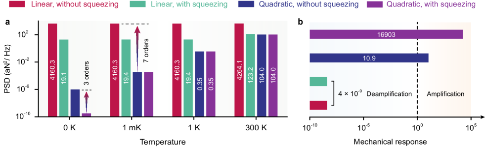
Figure 5: Comparisons of linear and quadratic COM sensors. a The optimal force sensitivity for linear and quadratic COM sensors at different temperatures. b The highest mechanical response for linear and quadratic COM sensors. The data of linear COM sensors are reproduced from ref. Zhao et al. (2020).

In standard phase detection ($\phi=\pi/2$), the output canonical quadratures are generally uncorrelated. As shown in Fig. 3a, the force sensitivity is constrained by the SQL in conventional COM system Zhao et al. (2020), where the symmetrized noise spectrum is simplified as (in the limit of $\kappa\gg\Omega$):

$$\bar{n}_{\mathrm{add}}^{\pi/2}\quantity[\Omega]=C+\frac{1}{16\eta_{c}C\Gamma_{m}^{2}\left|\chi_{m}\right|^{2}}\geq\frac{1}{2\sqrt{\eta_{c}}\Gamma_{m}\left|\chi_{m}\right|},$$ (3)

where the multi-photon cooperativity is defined as $C=4g^{2}/\quantity(\kappa\Gamma_{m})$, and $n_{c}=\Omega_{m}/\quantity(2g_{0})$ and $g=g_{0}\bar{q}_{m}\sqrt{2n_{c}}$ quantify the mean photon number and the effective optomechanical coupling rate, respectively. Hence, the SQL for a quadratic COM system reads:

$$\bar{n}_{\mathrm{add}}^{\mathrm{SQL}}\quantity[\Omega]=2C_{\mathrm{SQL}}\quantity[\Omega]=\frac{1}{2\sqrt{\eta_{c}}\Gamma_{m}\absolutevalue{\chi_{m}}}.$$ (4)

Its output noise spectrum can thus be determined by $\bar{S}_{\mathrm{FF}}^{\mathrm{SQL}}\quantity[\Omega]=2\hbar m_{\mathrm{eff}}\Gamma_{m}\Omega_{m}\bar{n}_{\mathrm{add}}^{\mathrm{SQL}}$. Due to such a pair of uncorrelated quadratures, the force sensitivity remains limited by the SQL, even including an intracavity squeezing medium with zero squeezing phase.

In contrast to the conventional phase detection, we show that the force noise can be squeezed well below the SQL by varying the squeezing phase and the homodyne angle, reaching the optimal squeezing degree of $35.2$ decibels (Fig. 3b). Counterintuitively, the quadratic COM sensor enables a remarkable amplification of the input force signal (Fig. 3b), due to its substantial improvement in the effective mechanical susceptibility (Fig. 1a-b). These features based on quadratic optomechanics is essentially different from the conventional enhancement of the SNR in a linear COM system, which relies on a larger reduction of the quantum noise than the suppressed detected signal Peano et al. (2015). Such a quantum non-demolition sensing process can be well characterized by the enhancement factor relating to the $\chi^{(2)}$ squeezing crystal:

$$\chi=\frac{\min\limits_{\phi,C}\quantity{\bar{n}_{\mathrm{add}}^{\phi}\left(G=0\right)}}{\min\limits_{\phi,C}\quantity{\bar{n}_{\mathrm{add}}^{\phi}\left(G\neq 0\right)}}.$$ (5)

In the vicinity of the optimal squeezing region, we achieve a $3$ orders of enhancement in sensitivity beyond the no squeezing case (Fig. 3c), which can be further improved by injecting squeezed vacuum into the COM system Lü et al. (2015); Qin et al. (2018). This high sensitivity is obtained close to the boundary between the stable and unstable regimes (see Supplementary Information for details). Thus, a decreased squeezing phase corresponds to a lower detection efficiency in the stable region (Fig. 3d), because of the narrower range for the multi-photon cooperativity. Further exploiting the interplay of the optical and mechanical parametric oscillations can access an even higher measurement precision, enabling a considerable enhancement in the SNR and a remarkable optimization for the performance of the noninvasive quantum sensors Levitan et al. (2016).

Figure 3e explores the thermal effect on sub-SQL detection for quadratic COM sensors. The increase of the mean phonon occupancy gives rise to a larger thermal mechanical motion and then lowers the sensing precision. However, we find that under realistic experimental conditions, the force sensitivity can still achieve $\quantity($10.2\text{\,}\mathrm{aN}$)^{2}$\mathrm{/}\mathrm{Hz}$$ at room temperature and reach $\quantity($1.9\text{\,}\mathrm{zN}$)^{2}$\mathrm{/}\mathrm{Hz}$$ at mean phonon occupations of $0.21$. These results are competitive with those obtained with the state-of-the-art sensors that have force noises in the range $10$ – $100\leavevmode\nobreak\ $\mathrm{a}\mathrm{N}\,\mathrm{Hz}^{-1/2}$$ at room temperature, and less than $1\text{\,}\mathrm{a}\mathrm{N}\,\mathrm{Hz}^{-1/2}$ at cryogenic temperatures Hälg et al. (2021). In Fig. 3f, we plot various noise contributions to the total power spectral density (PSD), which contains quantum backation and imprecision, internal losses or thermal noise. By leveraging quantum correlations between output optical quadratures, sub-SQL sensitivity can be achieved even in the presence of thermal noise and internal losses. This results in the zeptonewton force sensitivity near the motional ground state, which is well competitive with those achieved in the very recent experiments Mason et al. (2019); Catalini et al. (2020), with total noise of $\quantity($1.9\text{\,}\mathrm{aN}$)^{2}$\mathrm{/}\mathrm{Hz}$$ at $4\text{\,}\mathrm{K}$, and $\quantity($11.2\text{\,}\mathrm{aN}$)^{2}$\mathrm{/}\mathrm{Hz}$$ at $10\text{\,}\mathrm{K}$.

	Experiment		Mean phonon		Equivalent force
Sensors	(Y/N)	Temperature	occupations	Reported sensitivity	sensitivity	References
Accelerometer	Y	$3\text{\,}\mathrm{K}$	$2.3\text{\times}{10}^{6}$	$\quantity(10\leavevmode\nobreak\ $\mathrm{\SIUnitSymbolMicro}$g)^{2}$\mathrm{/}\mathrm{Hz}$$	$\quantity(13.7\leavevmode\nobreak\ $\mathrm{fN}$)^{2}$\mathrm{/}\mathrm{Hz}$$	Krause et al. (2012)
Accelerometer	Y	$300\text{\,}\mathrm{K}$	$4.0\text{\times}{10}^{9}$	$\quantity(32\leavevmode\nobreak\ $\mathrm{n}$g)^{2}$\mathrm{/}\mathrm{Hz}$$	$\quantity(3.4\leavevmode\nobreak\ $\mathrm{pN}$)^{2}$\mathrm{/}\mathrm{Hz}$$	Zhou et al. (2021)
Magnetometer	Y	$300\text{\,}\mathrm{K}$	$1.1\text{\times}{10}^{6}$	$\quantity(400\leavevmode\nobreak\ $\mathrm{nT}$)^{2}$\mathrm{/}\mathrm{Hz}$$	$\quantity(2.4\leavevmode\nobreak\ $\mathrm{pN}$)^{2}$\mathrm{/}\mathrm{Hz}$$	Forstner et al. (2012)
Magnetometer	Y	$300\text{\,}\mathrm{K}$	$1.2\text{\times}{10}^{6}$	$\quantity(200\leavevmode\nobreak\ $\mathrm{pT}$)^{2}$\mathrm{/}\mathrm{Hz}$$	$\quantity(1.2\leavevmode\nobreak\ $\mathrm{fN}$)^{2}$\mathrm{/}\mathrm{Hz}$$	Forstner et al. (2014)
Magnetometer	Y	$300\text{\,}\mathrm{K}$	$\sim$1.0\text{\times}{10}^{6}$$	$\quantity(5\leavevmode\nobreak\ $\mathrm{nT}$)^{2}$\mathrm{/}\mathrm{Hz}$$	$\quantity(0.75\leavevmode\nobreak\ $\mathrm{nN}$)^{2}$\mathrm{/}\mathrm{Hz}$$	Li et al. (2018)
Torque sensor	Y	$\sim$1\text{\,}\mathrm{mK}$$	$\sim 2.8$	$\quantity(1.3\leavevmode\nobreak\ $\mathrm{zN}\text{\,}\mathrm{m}$)^{2}$\mathrm{/}\mathrm{Hz}$$	$\quantity(0.43\leavevmode\nobreak\ $\mathrm{fN}$)^{2}$\mathrm{/}\mathrm{Hz}$$	Wu et al. (2014)
Ultrasound sensor	Y	$300\text{\,}\mathrm{K}$	$1.3\text{\times}{10}^{8}$	$\quantity(8\leavevmode\nobreak\ $\mathrm{\SIUnitSymbolMicro Pa}$)^{2}$\mathrm{/}\mathrm{Hz}$$	$\sim\quantity(370\leavevmode\nobreak\ $\mathrm{fN}$)^{2}$\mathrm{/}\mathrm{Hz}$$	Basiri-Esfahani et al. (2019)
Dark matter sensor	N	$10\text{\,}\mathrm{mK}$	$\sim$1.3\text{\times}{10}^{3}$$	$\sim\quantity(1\leavevmode\nobreak\ $\mathrm{p}$g)^{2}$\mathrm{/}\mathrm{Hz}$$	$\sim\quantity($67.4\text{\,}\mathrm{aN}$)^{2}$\mathrm{/}\mathrm{Hz}$$	Manley et al. (2021)
This work	N	$300\text{\,}\mathrm{K}$	$6.2\text{\times}{10}^{6}$	$\quantity($10.2\text{\,}\mathrm{aN}$)^{2}$\mathrm{/}\mathrm{Hz}$$
		$1\text{\,}\mathrm{K}$	$2.1\text{\times}{10}^{4}$	$\quantity($0.59\text{\,}\mathrm{aN}$)^{2}$\mathrm{/}\mathrm{Hz}$$
		$1\text{\,}\mathrm{mK}$	$20.8$	$\quantity($18.6\text{\,}\mathrm{zN}$)^{2}$\mathrm{/}\mathrm{Hz}$$
		$<$1\text{\,}\mathrm{mK}$$	$0.21$	$\quantity($1.9\text{\,}\mathrm{zN}$)^{2}$\mathrm{/}\mathrm{Hz}$$

Table 1: Extended applications to the state-of-the-art COM sensors. The resolution of the accelerometers is quantified by noise-equivalent acceleration in units of $g^{2}$\mathrm{/}\mathrm{Hz}$$, where $1\,g=$9.81\text{\,}\mathrm{m}\mathrm{/}\mathrm{s}^{2}$$.

Discussion

Recent development of components with ultralow mechanical dissipation is employed in gravitational-wave interferometers Yu et al. (2020) and at the nanoscale for measurement of weak forces Gavartin et al. (2012), where soft-clamping and strain engineering in mechanical resonators have allowed extremely high quality factors Tsaturyan et al. (2017); Ghadimi et al. (2018). Despite these achievements in improving the precision of quantum sensing, the process of quantum measurements is mainly limited by the thermal Langevin force, with spectral density given by the following fluctuation–dissipation theorem Tsaturyan et al. (2017):

$$\bar{S}_{\mathrm{FF}}=2m_{\mathrm{eff}}k_{\mathrm{B}}T\Omega_{m}/Q_{m},$$ (6)

where $k_{\mathrm{B}}$ is the Boltzmann’s constant, and $T$ is the temperature of the mechanical bath which can be reduced by placing the device in cryostats or dilution refrigerators. Written in this way, it is immediately evident that the fundamental thermal noise floor of a mechanical sensor benefits from a small mass and a large mechanical quality factor. One way of beating this classical limit is to use dissipation dilution Tsaturyan et al. (2017), specifically in amorphous materials such as silicon nitride (Fig. 4a). Compared with the fundamental approaches, our proposal achieves sub-SQL sensitivity near its motional ground state. For example, if hierarchical metamaterials are integrated into the MIM cavity Beccari et al. (a), the total force noise, consisting of thermal noise and quantum fluctuations, can be reduced to $\quantity($9.9\text{\,}\mathrm{zN}$)^{2}$\mathrm{/}\mathrm{Hz}$$ at the temperature of $0.2\text{\,}\mathrm{K}$ and $\quantity($70.5\text{\,}\mathrm{yN}$)^{2}$\mathrm{/}\mathrm{Hz}$$ at mean phonon occupations of $0.21$. These results indicate that quantum force sensors fabricated very recently with advanced approaches, can be further improved by utilizing quadratic instead of linear COM coupling (Fig. 4b).

In Fig. 5a, we show that even without any optical squeezing, the sensitivity of quadratic COM systems can still be higher than that of a linear COM sensor utilizing squeezed light. The resulting giant enhancement of sensitivity is due to the amplification of the signal imprinted on the quadratures, which can lead to $9$ orders of enhancement in the mechanical response beyond linear COM sensors (Fig. 5b). We also note that quadratic COM sensors are dominated by thermal noise even at millikelvin temperatures, due to its substantially suppressed quantum fluctuations.

To summarize, we show that quantum force sensing can be significantly improved by using quadratic COM devices, in comparison with conventional linear COM sensors. Further integrating it with an intracavity squeezing medium can lead to further enhancement of force sensitivity, reaching the zeptonewton level. This opens new prospects of making and using quantum nonlinear COM sensors in fundamental physics experiments and in a wide range of practical fields requiring extreme sensitivity de Jong et al. (2022); Fogliano et al. (2021b); Liu et al. (2016); Jing et al. (2011).

Methods

Extended applications to precision measurements

Table 1 provides a comparison of performance metrics for recently reported COM sensors including the force sensor described in this work.

Theoretical model

In the standard linearized process (under strong optical drives), the resulting quantum Langevin equations are given by

$$\begin{pmatrix}\delta\dot{\hat{\mathbf{Q}}}_{c}\\ \delta\dot{\hat{\mathbf{Q}}}_{m}\end{pmatrix}=\begin{pmatrix}\mathbf{A}&\mathbf{B}\\ \mathbf{B}&\mathbf{C}\end{pmatrix}\begin{pmatrix}\delta\hat{\mathbf{Q}}_{c}\\ \delta\hat{\mathbf{Q}}_{m}\end{pmatrix}+\begin{pmatrix}\delta\hat{\mathbf{S}}_{\mathrm{in}}\\ \delta\hat{\mathbf{F}}_{\mathrm{in}}\end{pmatrix},$$ (7)

where the canonical optical quadrature operators are defined as $\delta\hat{q}_{c}=\left(\delta\hat{a}+\delta\hat{a}^{\dagger}\right)/\sqrt{2}$, $\delta\hat{p}_{c}=\left(\delta\hat{a}-\delta\hat{a}^{\dagger}\right)/(\sqrt{2}\mathrm{i})$, respectively, and the associated matrices are given by

$$\sigma_{\pm} =\Delta\pm 2G\sin\theta, \rho_{\pm} \left.=\kappa\middle/2\pm 2G\cos\theta,\right.$$

$$\hat{\mathbf{Q}}_{c} =\begin{pmatrix}\hat{q}_{c}&\hat{p}_{c}\end{pmatrix}^{\mathrm{T}}, \hat{\mathbf{Q}}_{m} =\begin{pmatrix}\hat{q}_{m}&\hat{p}_{m}\end{pmatrix}^{\mathrm{T}},$$

$$\hat{\mathbf{S}}_{\mathrm{in}} =\mathbf{D}\mathbf{E}, \hat{\mathbf{F}}_{\mathrm{in}} =\begin{pmatrix}0&\sqrt{2\Gamma_{m}}\hat{F}_{\mathrm{in}}\end{pmatrix}^{\mathrm{T}},$$

$$\mathbf{M} =\begin{pmatrix}\mathbf{A}&\mathbf{B}\\ \mathbf{B}&\mathbf{C}\end{pmatrix}, \mathbf{A} =\begin{pmatrix}-\rho_{-}&\sigma_{+}\\ -\sigma_{-}&-\rho_{+}\end{pmatrix},$$

$$\mathbf{B} =\begin{pmatrix}0&0\\ 2g&0\end{pmatrix}, \mathbf{C} =\begin{pmatrix}0&\Omega_{m}\\ 0&-\Gamma_{m}\end{pmatrix},$$

$$\mathbf{D} =\begin{pmatrix}\hat{q}_{\mathrm{in}}&\hat{q}_{0}\\ \hat{p}_{\mathrm{in}}&\hat{p}_{0}\end{pmatrix}, \mathbf{E} =\begin{pmatrix}\sqrt{\eta_{c}\kappa}\\ \sqrt{\left(1-\eta_{c}\right)\kappa}\end{pmatrix}.$$ (8)

In the Fourier domain, using the input-output relations, $\delta\hat{\mathbf{Q}}_{\mathrm{out}}\left[\Omega\right]=\sqrt{\eta_{c}\kappa}\delta\hat{\mathbf{Q}}_{c}\left[\Omega\right]-\delta\hat{\mathbf{Q}}_{\mathrm{in}}\left[\Omega\right]$, the quadratures of the output optical field can be written as

$$\delta\hat{\mathbf{Q}}_{\mathrm{out}}\left[\Omega\right]=\mathcal{L}\left[\Omega\right]\delta\hat{\mathbf{V}}_{\mathrm{in}}\left[\Omega\right],$$ (9)

where

$$\hat{\mathbf{Q}}_{\mathrm{out}}\left[\Omega\right] =\begin{pmatrix}\hat{q}_{\mathrm{out}}&\hat{p}_{\mathrm{out}}\end{pmatrix}^{\mathrm{T}},$$

$$\hat{\mathbf{V}}_{\mathrm{in}}\left[\Omega\right] =\begin{pmatrix}\hat{q}_{\mathrm{in}}&\hat{p}_{\mathrm{in}}&\hat{q}_{0}&\hat{p}_{0}&\hat{F}_{\mathrm{in}}\end{pmatrix}^{\mathrm{T}},$$

$$\mathcal{L}\left[\Omega\right] =\begin{pmatrix}\mathcal{A}_{-}&\mathcal{B}_{-}&\mathcal{C}_{-}&\mathcal{D}_{-}&\mathcal{N}_{-}\\ -\mathcal{B}_{+}&\mathcal{A}_{+}&-\mathcal{D}_{+}&\mathcal{C}_{+}&\mathcal{N}_{+}\end{pmatrix}.$$ (10)

The input term of external forces are described as $\hat{F}_{\mathrm{in}}=\hat{F}_{\mathrm{th}}+\hat{F}_{\mathrm{sig}}$, where $\hat{F}_{\mathrm{th}}=\hat{\mathcal{F}}_{\mathrm{th}}\big{/}\sqrt{2\hbar m_{\mathrm{eff}}\Gamma_{m}\Omega_{m}}$ and $\hat{F}_{\mathrm{sig}}=\hat{\mathcal{F}}_{\mathrm{sig}}\big{/}\sqrt{2\hbar m_{\mathrm{eff}}\Gamma_{m}\Omega_{m}}$ are the scaled thermal force and detected force signal with dimension $\mathrm{Hz}^{\left.1\middle/2\right.}$, respectively. The variables $\delta\hat{a}_{\mathrm{in}}$ and $\delta\hat{a}_{{}_{0}}$ represent the fluctuations at the coupling port and the port modelling internal losses, respectively. The associated coefficients in Eq. (Theoretical model) are given in Supplementary Information, and the effective susceptibilities of the optical and mechanical modes are defined as $\chi_{\pm}\quantity[\Omega]=\quantity(\rho_{\pm}-\mathrm{i}\Omega)^{-1}$, $\chi_{m}\left[\Omega\right]=-\Omega_{m}/\quantity(\Omega^{2}+\mathrm{i}\Omega\Gamma_{m})$, respectively. We note that this mechanical susceptibility is different from the conventional Lorentzian susceptibility for a linear COM system Sudhir et al. (2017), which is defined as $\chi_{s}\quantity[\Omega]=\Omega_{m}/(\Omega_{m}^{2}-\Omega^{2}-\mathrm{i}\Omega\Gamma_{m})$. This indicates that the force signal in a quadratic system is transduced more efficiently into the displacement than that in a linear COM system (see Supplementary Information for details) Sudhir et al. (2017).

Data availability

The numerical data generated in this work is available from the authors upon reasonable request.

References

Author contributions

S.-D.Z. performed the calculations. S.-D.Z., J.W., Y.-F.J., H.Z., Y.L., Y.-L.Z, Ş.K.Ö., C.-W.Q., F.N. and H.J. discussed the results and wrote the paper. H.J. conceived the idea and supervised the project.

Competing interests

The authors declare no competing interests.

Supplementary Information for:
Zeptonewton force sensing with squeezed quadratic optomechanics

Sheng-Dian Zhang,¹ Jie Wang,¹ Ya-Feng Jiao,¹ Huilai Zhang,¹ Ying Li,¹

Yun-Lan Zuo,¹ Şahin K. Özdemir,² Cheng-Wei Qiu,³ Franco Nori,^4, 5 and Hui Jing${}^{1,\,*}$

¹Key Laboratory of Low-Dimensional Quantum Structures and Quantum Control of Ministry of Education,
Department of Physics and Synergetic Innovation Center for Quantum Effects
and Applications, Hunan Normal University, Changsha 410081, China
²Department of Engineering Science and Mechanics, and Materials Research Institute,
Pennsylvania State University, University Park, State College, Pennsylvania 16802, USA
³Department of Electrical and Computer Engineering,
National University of Singapore, Singapore 117583, Singapore
⁴Theoretical Quantum Physics Laboratory, RIKEN Cluster for Pioneering Research, Wako-shi, Saitama 351-0198, Japan
⁵Physics Department, The University of Michigan, Ann Arbor, Michigan 48109-1040, USA
^∗ To whom correspondence should be addressed; E-mail: jinghui73@foxmail.com
(Dated: March 7, 2024)

Here, we present more technical details on quantum squeezed sensing with quadratic optomechanics, including: (1) nonlinear coupling between the pump mode and the second-harmonic mode; (2) detailed derivations of the linearized Hamiltonian; (3) more discussions on stability conditions, especially the conversion of stability and instability; (4) noise spectrum and mechanical response characterizations; (5) reconstructed Wigner function and theoretical analysis of quantum advantage; (6) signal-to-noise ratio and the optimal variance of the rotated field quadrature; (7) main hurdles to quantum-noise-limited measurements; (8) the effect of the fluctuations of the second-harmonic mode; (9) analysis of the validity of the high-temperature approximation; (10) a summary of all experimentally accessible parameters used in our work.

Supplementary Note 1:  Second-order nonlinear processes

The second-harmonic generation (SHG) in our system can arise from the quadratic response of the media electric dipoles and multipoles $\mathbf{P}^{(2)}$ to the external field $\mathbf{E}$. The total second-order nonlinear electric polarization can thus be expressed as Strekalov et al. (2016)

$$\mathbf{P}^{(2)}_{i}=\sum_{j,k}\chi_{ijk}^{(2)}\mathbf{E}_{j}\mathbf{E}_{k},$$ (1)

where $\chi^{(2)}$ is the nonlinear susceptibility tensor, and $i$, $j$, $k$ denote the crystallographic axes $x$, $y$, $z$, respectively. Using the Helmholtz equation for the SH electric field $\mathbf{E}_{p}$, we obtain

$$\quantity(\laplacian-\frac{n_{p}^{2}}{c^{2}}\partialderivative[2]{t})\mathbf{E}_{p}=\frac{1}{c^{2}}\partialderivative[2]{\mathbf{P}^{(2)}}{t},$$ (2)

where $n_{p}$ is the refractive index for the SH mode, and $c$ is the speed of light in vacuum. Under the slowly varying approximation and the electromagnetic field quantization Strekalov et al. (2016); Zhang et al. (2018), the dynamic evolution of the SH mode reads $\dot{\hat{a}}_{p}=\mathrm{i}\nu\hat{a}_{s}^{2}\exp[-\mathrm{i}\quantity(\Omega_{p}-2\Omega_{s})t]$, where we have replaced $\Omega_{c}$ with $\Omega_{s}$. The second-order nonlinear strength is then given by Zhang et al. (2018)

$$\nu=\frac{2\Omega_{s}^{2}}{\Omega_{p}n_{p}^{2}}\frac{\int\mathbf{E}_{0p}^{*}\cdot\mathbf{P}^{(2)}\differential V}{\int\absolutevalue{\mathbf{E}_{0p}}^{2}\differential V},$$ (3)

where $\mathbf{E}_{0p}$ represents the normalized spatial field distribution of the SH mode.

In the case of strong optical drives, the squeezing strength is derived from the steady-state equations:

$$G=\nu\quantity(\tau-\sqrt{\tau^{2}+\frac{\Omega_{m}}{8g_{0}}-\frac{\absolutevalue{\varepsilon_{p}}}{4\nu}}),$$ (4)

where $\tau=\sqrt{\kappa^{2}+4\Delta_{p}^{2}}/\quantity(16\nu)$, $\absolutevalue{\varepsilon_{p}}=\sqrt{\kappa\eta_{c}P_{p}/\quantity(2\hbar\Omega_{l})}$, and $P_{p}$ quantifies the pump power for the SH mode. As the SH power and the second-order nonlinearity increase, the squeezing strength is improved to the range of the sensitive region (Supplementary Fig. 1a, left panel), following the characteristic optical parametric oscillation (OPO) power curve Bruch et al. (2019). However, when increasing the detuning of the pump laser, the photons circulating in the cavity reduce, which results in the suppression of the squeezing strength (Supplementary Fig. 1a, right panel). Supplementary Fig. 1b schematically illustrates the $\chi^{(2)}$ nonlinear process, where the OPO model can be treated as two coupled cavities with spontaneous parametric down-conversion Bruch et al. (2019). The visible pump laser at frequency $\Omega_{p}$ drives the cavity, producing a pair of infrared signal and idler modes at frequencies $\Omega_{s}$ and $\Omega_{i}$, which satisfies the energy-matching condition $\Omega_{p}=\Omega_{s}+\Omega_{i}$. For degenerate OPOs ($\Omega_{s}=\Omega_{i}=\Omega_{p}/2$), a single parametric oscillation is realized at half the frequency of the pump laser. Whereas for non-degenerate cases ($\Omega_{s}\neq\Omega_{i}$), the OPO process is operated at two distinct resonances centered about the pump.

In Table 1, we summarize the performances of the recent $\chi^{(2)}$ nonlinear experiments, for their respective state-of-the-art OPOs in terms of the material, refractive index, pump power, $Q$ factor, operating wavelengths, nonlinear coefficients and processes, and device structures and sizes. The squeezed light used in our proposed scheme can be generated with various nonlinear on-chip devices, such as superconducting qubits Eddins et al. (2019), photonic crystals Marty et al. (2021) and layered semiconducting materials Trovatello et al. (2021).

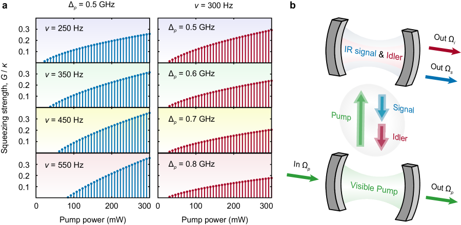
Supplementary Figure 1: Degenerate OPO process. a The squeezing strength versus on-chip pump power for the parametric oscillation process. The evolutions are shown at a red detuning of the SH mode with $\Delta_{p}=$0.5\text{\,}\mathrm{GHz}$$ (left panel) Peano et al. (2015) and a second-order nonlinearity of $\nu=$300\text{\,}\mathrm{Hz}$$ (right panel) Bruch et al. (2019). The theoretical pump power threshold is tens of milliwatts, which is in agreement with the recent OPO experiment Bruch et al. (2019). b Schematic representation of the OPO model using two Fabry–Pérot cavities.

Material			Geometry	Nonlinear	Size ($\mathrm{\SIUnitSymbolMicro m}$): rings: $r/w/h$,	$\lambda_{p}-\lambda_{s}$ ($\mathrm{nm}$)	Quality	Pump	References
	Refractive	$\chi^{(2)}$		process	waveguides: $L/w/h$,		factor	power
	index	($\mathrm{p}\mathrm{m}\mathrm{/}\mathrm{V}$)		(SHG/SFG)	disks: $r/h$, and spheres: $r$		($\times 10^{6}$)	($\mathrm{mW}$)
Table-top OPO	–	–	Crystal-based	SHG	–	$780-1560$	$11$	$300$	This work
Table-top OPO	–	–	Crystal-based	SHG	–	$532-1064$	–	$350$	Vahlbruch et al. (2016)
Si3N4	–	$0.2$	Microring	SHG	$23/1.2/0.6$	$780-1560$	$1.2$	$15$	Lu et al. (2021a)
AlN	–	–	Microring	SFG	$30/1.2/1.1$	$780-1560$	$1.38$	$23$	Wang et al. (2021)
AlN	–	$1.3$	Microring	SFG	$30/1.12/1.0$	$773-1556$	$0.18$	$24.4$	Guo et al. (2016)
AlN	$2.1$	$6$	Microring	SHG	$60/1.2/1.0$	$780-1560$	$1.0$	$12$	Bruch et al. (2019)
LiNbO3	–	–	Microring	SHG	$50/0.69/0.55$	$775-1550$	$0.14$	$0.105$	Luo et al. (2019)
LiNbO3	–	$0.6$	Microring	SFG	$80/1.6/0.6$	–	$0.9$	$20$	Xu et al. (2021)
PPLN	$2.2$	$40$	Microring	SHG	–	$775-1550$	$0.6$	$0.03$	Lu et al. (2021b)
LiNbO3	$2.21$	$2.1$	Microdisk	SHG	$51/0.7$	$770-1540$	$0.11$	$10$	Lin et al. (2016)
GaP	–	–	Microdisk	SHG	$3.3/0.25$	$772-1545$	$0.11$	$0.35$	Lake et al. (2016)
SiO2	–	–	Microsphere	SHG	$62$	$775-1550$	$48$	$0.879$	Zhang et al. (2018)
LiNbO3	–	–	$\mathrm{mm}$-Resonator	SHG	$1900/500$	$532-1064$	$34$	$0.03$	Fürst et al. (2010)
PPLN	$2.138$	$0.023$	$\mathrm{mm}$-Resonator	SHG	$1500/500$	$775-1550$	$12$	$300$	Ilchenko et al. (2004)
PPLN	–	–	Waveguide	SHG	$4000/1.4/0.6$	$775-1550$	–	$100$	Wang et al. (2018)
PPLN	–	–	Waveguide	SHG	$30000/6/...$	$780-1560$	–	$40$	Mondain et al. (2019)

Supplementary Table 1: Performances of nonlinear integrated platforms for OPOs. PPLN: periodically poled LiNbO3.

Supplementary Note 2:  Derivation of the linearized Hamiltonian

In our cavity optomechanical (COM) system, the pump laser with frequency $2\Omega_{l}$ has twice the frequency of the signal laser. Such a visible laser drives the fundamental (FM) mode resonantly but is detuned with respect to the second-harmonic (SH) mode Peano et al. (2015). The flexible dielectric membrane is placed at a location of $\left.q_{0}=j\lambda_{p}\middle/4=k\lambda_{s}\middle/4\right.$ ($j$, $k$ integers) Bhattacharya et al. (2008), i.e., the common node (or antinode) of the intracavity standing waves Sankey et al. (2010), where $\lambda_{p}$ and $\lambda_{s}$ are the resonant wavelengths for the SH and FM modes, respectively. We then form a realistic description incorporating intrinsic losses and the coupling of the mechanical resonator to the optical modes, which yields the total Hamiltonian in a rotating frame Thompson et al. (2008); Peano et al. (2015):

$$\hat{H} =\hbar\Delta_{c}\hat{a}_{s}^{\dagger}\hat{a}_{s}+\hbar\Delta_{p}\hat{a}_{p}^{\dagger}\hat{a}_{p}+\frac{\hbar}{2}\Omega_{m}\quantity(\hat{q}_{m}^{2}+\hat{p}_{m}^{2})-\hbar\hat{q}_{m}^{2}\quantity(g_{s}\hat{a}_{s}^{\dagger}\hat{a}_{s}+g_{p}\hat{a}_{p}^{\dagger}\hat{a}_{p})$$

$$\quad+\mathrm{i}\hbar\nu\quantity(\hat{a}_{s}^{\dagger 2}\hat{a}_{p}\mathrm{e}^{\mathrm{i}\theta}-\hat{a}_{s}^{2}\hat{a}_{p}^{\dagger}\mathrm{e}^{-\mathrm{i}\theta})+\mathrm{i}\hbar\quantity(\varepsilon_{c}\hat{a}_{s}^{\dagger}+\varepsilon_{p}\hat{a}_{p}^{\dagger}-\mathrm{H.C.}),$$ (5)

where we have applied the unitary transformation $\hat{U}\quantity(t)=\exp[\mathrm{i}\Omega_{l}t\quantity(\hat{a}_{s}^{\dagger}\hat{a}_{s}+2\hat{a}_{p}^{\dagger}\hat{a}_{p})]$, and the driving amplitudes are $\absolutevalue{\varepsilon_{c}}=\sqrt{\kappa_{s}\eta_{c}P_{s}/(\hbar\Omega_{l})}$, $\absolutevalue{\varepsilon_{p}}=\sqrt{\kappa_{p}\eta_{p}P_{p}/(2\hbar\Omega_{l})}$. The detunings of the optical modes are $\Delta_{c}=\Omega_{c}-\Omega_{l}$ and $\Delta_{p}=\Omega_{p}-2\Omega_{l}$, with $g_{s}$ and $g_{p}$ the COM coupling strength of the FM and SH modes, respectively. The effect of the second-order pump mode can be treated classically with proper conditions (see Supplementary Note 8). Within these experimentally accessible approximations, the linearized Heisenberg-Langevin equations under strong optical drives are

$$\delta\dot{\hat{a}} =-\left(\mathrm{i}\Delta+\frac{\kappa}{2}\right)\delta\hat{a}+2G\mathrm{e}^{\mathrm{i}\theta}\delta\hat{a}^{\dagger}+\sqrt{2}\mathrm{i}g\delta\hat{q}_{m}+\sqrt{\eta_{c}\kappa}\delta\hat{a}_{\mathrm{in}}+\sqrt{\left(1-\eta_{c}\right)\kappa}\delta\hat{a}_{0},$$

$$\delta\dot{\hat{q}}_{m} =\Omega_{m}\delta\hat{p}_{m},$$

$$\delta\dot{\hat{p}}_{m} =-\Gamma_{m}\delta\hat{p}_{m}+\sqrt{2}g\left(\delta\hat{a}+\delta\hat{a}^{\dagger}\right)+\sqrt{2\Gamma_{m}}\delta\hat{F}_{\mathrm{in}},$$ (6)

where $\Delta=\Delta_{c}-g_{0}\bar{q}_{m}^{2}$, $n_{c}=\left|\alpha\right|^{2}$, $g=g_{0}\bar{q}_{m}\sqrt{2n_{c}}$, and $\hat{a}_{s}$ and $g_{s}$ are replaced with $\hat{a}$ and $g_{0}$, respectively. The single-photon coupling rate is denoted by $g_{0}=g_{\mathrm{om}}q_{\mathrm{zp}}^{2}$, and the quadratic coupling strength reads Bhattacharya et al. (2008): $g_{\mathrm{om}}=8\pi^{2}c\sqrt{R/\quantity(1-R)}/\quantity(\lambda_{s}^{2}L)$, which can reach $1.54\text{\,}\mathrm{T}\mathrm{Hz}\mathrm{/}\mathrm{n}\mathrm{m}^{2}$ in experiment Paraïso et al. (2015). Such a position-squared COM coupling has allowed for novel quantum effects, such as photon blockade Liao and Nori (2014), phonon condensate Zheng and Li (2021), and quantum nonreciprocity Xu et al. (2020). Here, for simplicity, we define the dimensionless mechanical quadratures as $\left.\hat{q}_{m}=\hat{q}\middle/q_{\mathrm{zp}}\right.$ and $\left.\hat{p}_{m}=\hat{p}\middle/p_{\mathrm{zp}}\right.$, where $q_{\mathrm{zp}}=\sqrt{\hbar/(m_{\mathrm{eff}}\Omega_{m})}$, $p_{\mathrm{zp}}=\sqrt{\hbar m_{\mathrm{eff}}\Omega_{m}}$ are the standard deviations of the zero-point motion and momentum, respectively. Besides, the FM mode is characterized by a total loss rate $\kappa=\kappa_{0}+\kappa_{\mathrm{ex}}$ with the cavity coupling parameter $\left.\eta_{c}=\kappa_{\mathrm{ex}}\middle/\left(\kappa_{0}+\kappa_{\mathrm{ex}}\right)\right.$. We note that in a very recent experiment Bruch et al. (2019), the second-order nonlinearity has reached a value of $\nu/2\pi=$80\text{\,}\mathrm{kHz}$$. Thus, it is possible to generate a squeezing strength of $G=\nu\alpha_{p}=0.25\kappa$ (Supplementary Fig. 1a), where $\alpha_{p}$ denotes the average amplitude of the SH mode, and $\theta$ qualifies the squeezing phase of the nonlinear crystal that contributes to noise reduction and enhancement Yap et al. (2020).

Without loss of generality Peano et al. (2015), we choose $\alpha_{p}\in\mathbb{R}>0$, and take intracavity field as the phase reference, i.e., $\alpha\in\mathbb{R}>0$. The solutions of the steady-state values can thus be expressed as

$$\cos\theta =\frac{1}{4G}\left(\kappa-\left|\frac{2\varepsilon_{c}}{\sqrt{n_{c}}}\right|\cos\Phi\right),$$

$$\bar{q}_{m}^{2} =\frac{1}{g_{0}}\left(\Delta_{c}-\left|\frac{\varepsilon_{c}}{\sqrt{n_{c}}}\right|\sin\Phi-2G\sin\theta\right),$$ (7)

where $n_{c}=\Omega_{m}/\quantity(2g_{0})$, and the squeezing angle depends on the phase $\Phi$ of the signal laser. Then, the displacement of the oscillator is directly proportional to the input force signal:

$$\delta\hat{q}\quantity[\Omega]=\chi_{\mathrm{eff}}^{(2)}\quantity[\Omega]\delta\hat{\mathcal{F}}_{\mathrm{sig}}\quantity[\Omega],$$ (8)

where $\chi_{\mathrm{eff}}^{(2)}\quantity[\Omega]$ denotes the effective mechanical susceptibility Gavartin et al. (2012):

$$\chi_{\mathrm{eff}}^{(2)}\quantity[\Omega]=\frac{1}{m_{\mathrm{eff}}\Omega_{m}\quantity(\chi_{m}^{-1}+\Sigma)},\qquad\Sigma\quantity[\Omega]=\frac{16g^{2}\quantity(\Omega-\Delta-2G\sin\theta)}{\kappa^{2}-16G^{2}+4\quantity(\Omega-\Delta)^{2}}.$$ (9)

For the resonance case without intracavity squeezing Gavartin et al. (2012), the additional term $\Sigma\quantity[\Omega]$ can be neglected. The effective susceptibility thus has the simplest form:

$$\chi_{\mathrm{eff}}^{(2)}\quantity[\Omega]=-\frac{1}{m_{\mathrm{eff}}\quantity(\Omega^{2}+\mathrm{i}\Omega\Gamma_{m})}.$$ (10)

The time-varying equation (2) can be solved in the Fourier domain (see the Methods), where the corresponding matrices and coefficients are given by

$$\tau\quantity[\Omega] =\sigma_{-}-4g^{2}\chi_{m}, \rho\quantity[\Omega] =\left(1+\tau\sigma_{+}\chi_{+}\chi_{-}\right)^{-1},$$

$$\mathcal{A}_{\pm}\quantity[\Omega] =\kappa\rho\chi_{\pm}\eta_{c}-1, \mathcal{B}_{+}\quantity[\Omega] =\kappa\rho\tau\chi_{+}\chi_{-}\eta_{c},$$

$$\mathcal{B}_{-}\quantity[\Omega] =\sigma_{+}\mathcal{B}_{+}/\tau, \mathcal{C}_{\pm}\quantity[\Omega] =\kappa\rho\chi_{\pm}\sqrt{\eta_{c}\left(1-\eta_{c}\right)},$$

$$\mathcal{D}_{+}\quantity[\Omega] =\kappa\rho\tau\chi_{+}\chi_{-}\sqrt{\eta_{c}\left(1-\eta_{c}\right)}, \mathcal{D}_{-}\quantity[\Omega] =\sigma_{+}\mathcal{D}_{+}/\tau,$$

$$\mathcal{N}_{+}\quantity[\Omega] =2\rho g\chi_{+}\chi_{m}\sqrt{2\kappa\eta_{c}\Gamma_{m}}, \mathcal{N}_{-}\quantity[\Omega] =\sigma_{+}\chi_{-}\mathcal{N}_{+}.$$ (11)

Supplementary Note 3:  Stability conditions

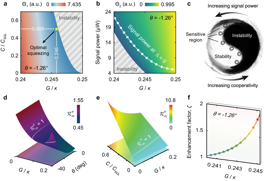
Supplementary Figure 2: Stability analysis and mechanical response. a-b Stability functions $\Theta_{1}$ and $\Theta_{2}$. The yellow star, which denotes the optimal squeezing in the main text, locates at the stable zone. The white curve represents the required signal power on the resonance, which is truly stable and experimentally accessible. c Schematics of the sensitive stable region. Stability and instability can be converted into each other by altering the signal power or the muti-photon cooperativity. The sensitive data are thus distributed in the vicinity of the dividing line. d-f Mechanical response and its enhancement compared with standard phase detection. The force signal can be amplified on the output detected quadratures. The white curves denote $\mathcal{R}_{m}^{\phi}\quantity[\Omega]=1$.

The stability or instability of the system is determined by the signs of the real parts of the eigenvalues of the dynamical evolution matrix $\mathbf{M}$ (given in the Methods). To find the eigenvalues $\lambda$, it is necessary to solve the characteristic equation $\det(\mathbf{M}-\lambda\mathbf{I})=0$, which is reduced to an algebraic equation of the 4th degree: $\lambda^{4}+\mathrm{M}_{3}\lambda^{3}+\mathrm{M}_{2}\lambda^{2}+\mathrm{M}_{1}\lambda+\mathrm{M}_{0}=0$. Applying the Routh-Hurwtiz method, we obtain the necessary and sufficient conditions for the system stability:

$$0 <\mathrm{M}_{3}, 0 <\mathrm{M}_{3}\mathrm{M}_{2}-\mathrm{M}_{1},$$

$$0 <\mathrm{M}_{0}, 0 <\mathrm{M}_{3}\mathrm{M}_{2}\mathrm{M}_{1}-\left(\mathrm{M}_{1}^{2}+\mathrm{M}_{3}^{2}\mathrm{M}_{0}\right).$$ (12)

These conditions allow to determine whether all the roots in the characteristic equation have negative real parts. Thus, we can use them to justify the system stability without solving the characteristic equation itself. Herein, we focus on the resonance case ($\Delta\approx\Delta_{c}=0$), thereby the first three inequalities in Eq. (3) yield the first two stability conditions: $\left.G\middle/\kappa<0.25\right.$, $-\pi<\theta<0$. To proceed, we formulate the stability criterion functions $\Theta_{j}$ ($j=1,2$), according to the last inequality in Eq. (3) and $\absolutevalue{\cos\Phi}\leq 1$ in Eq. (2), as follows:

$$\Theta_{1}=\mathrm{M}_{3}\mathrm{M}_{2}\mathrm{M}_{1}-\left(\mathrm{M}_{1}^{2}+\mathrm{M}_{3}^{2}\mathrm{M}_{0}\right),\qquad\Theta_{2}=1-\quantity|\frac{\sqrt{n_{c}}}{2\varepsilon_{c}}\left(\kappa-4G\cos\theta\right)|.$$ (13)

Then, the signs of $\Theta_{j}$ provide the remaining stability requirements:

$$\mathrm{sgn}\left(\Theta_{j}\right)=\begin{cases}1,&\text{implies stability},\\ \text{otherwise},&\text{implies instability}.\end{cases}$$ (14)

As shown in Supplementary Fig. 2, the parameters used in our numerical calculations, are chosen truly in the stable region. In particular, the required signal power can be derived from Eq. (2):

$$P_{s}=\frac{\hbar\Omega_{l}n_{c}}{4\kappa\eta_{c}}\quantity[\quantity(\kappa-4G)^{2}+8G\kappa\quantity(1-\cos\theta)],$$ (15)

which is tens of microwatts and can be attained with current experimental conditions Zhang et al. (2018). Moreover, the multi-photon cooperativity on the resonance reads $C=-4\Omega_{m}\Delta/\quantity(\kappa\Gamma_{m})$, indicating that the effective COM coupling is independent of the nonlinear crystal. Hence, the improved force sensitivity is solely induced by the squeezed fluctuations rather than the enhanced COM coupling Lü et al. (2015). Supplementary Fig. 2c shows the transition from stability to instability or vice versa. In principle, a system tends to be sensitive to external perturbations in the unstable region. Then, the sensitive region in the stable realm locates near the dividing line between stability and instability.

Supplementary Note 4:  Noise spectral density

The output amplitude and phase fluctuations, as well as the correlations between the imprecision and the quantum backaction, can be expressed in terms of the symmetrized correlation and cross-correlation spectrum Sudhir et al. (2017):

$$\bar{S}_{\mathrm{qq}}^{\mathrm{out}}\left[\Omega\right] =\frac{1}{2}\left\langle\anticommutator{\delta\hat{q}_{\mathrm{out}}\left[\Omega\right]}{\delta\hat{q}_{\mathrm{out}}\left[-\Omega\right]}\right\rangle=\frac{1}{2}\mathcal{K}_{-}\left[\Omega\right]+\mathcal{R}_{-}\left[\Omega\right]\bar{n}_{m}^{T},$$

$$\bar{S}_{\mathrm{pp}}^{\mathrm{out}}\left[\Omega\right] =\frac{1}{2}\left\langle\anticommutator{\delta\hat{p}_{\mathrm{out}}\left[\Omega\right]}{\delta\hat{p}_{\mathrm{out}}\left[-\Omega\right]}\right\rangle=\frac{1}{2}\mathcal{K}_{+}\left[\Omega\right]+\mathcal{R}_{+}\left[\Omega\right]\bar{n}_{m}^{T},$$

$$\bar{S}_{\mathrm{pq}}^{\mathrm{out}}\left[\Omega\right] =\frac{1}{2}\left\langle\anticommutator{\delta\hat{q}_{\mathrm{out}}\left[\Omega\right]}{\delta\hat{p}_{\mathrm{out}}\left[-\Omega\right]}\right\rangle=\Re{\frac{1}{2}\mathcal{K}_{\mathrm{co}}\left[\Omega\right]+\mathcal{R}_{\mathrm{si}}\left[\Omega\right]\bar{n}_{m}^{T}},$$ (16)

respectively, where

$$\mathcal{R}_{\pm}\left[\Omega\right] =\left|\mathcal{N}_{\pm}\left[\Omega\right]\right|^{2}, \mathcal{R}_{\mathrm{si}}\left[\Omega\right] =\mathcal{N}_{+}^{*}\left[\Omega\right]\mathcal{N}_{-}\left[\Omega\right],$$

$$\mathcal{K}_{\mathrm{co}}\left[\Omega\right] =\mathcal{K}_{\mathrm{cr}}\left[\Omega\right]+\mathrm{i}\mathcal{K}_{\mathrm{si}}\left[\Omega\right], \mathbb{U}_{\pm}\left[\Omega\right] =\left|\mathcal{A}_{\pm}\left[\Omega\right]\right|^{2}+\left|\mathcal{B}_{\pm}\left[\Omega\right]\right|^{2},$$

$$\mathbb{V}_{\pm}\left[\Omega\right] =\left|\mathcal{C}_{\pm}\left[\Omega\right]\right|^{2}+\left|\mathcal{D}_{\pm}\left[\Omega\right]\right|^{2}, \mathbf{K}\left[\Omega\right] =\mathbf{U}\left[\Omega\right]+\mathbf{V}\left[\Omega\right],$$

$$\mathbf{K}\left[\Omega\right] =\begin{pmatrix}\mathcal{K}_{\pm}\left[\Omega\right]&\mathcal{K}_{\mathrm{cr}}\left[\Omega\right]&\mathcal{K}_{\mathrm{si}}\left[\Omega\right]\end{pmatrix}^{\mathrm{T}}, \mathbf{U}\left[\Omega\right] =\begin{pmatrix}\mathbb{U}_{\pm}\left[\Omega\right]&\mathbb{U}_{\mathrm{cr}}\left[\Omega\right]&\mathbb{U}_{\mathrm{si}}\left[\Omega\right]\end{pmatrix}^{\mathrm{T}},$$

$$\mathbf{V}\left[\Omega\right] =\begin{pmatrix}\mathbb{V}_{\pm}\left[\Omega\right]&\mathbb{V}_{\mathrm{cr}}\left[\Omega\right]&\mathbb{V}_{\mathrm{si}}\left[\Omega\right]\end{pmatrix}^{\mathrm{T}}, \begin{pmatrix}\mathbb{U}_{\mathrm{si}}\left[\Omega\right]\\ \mathbb{U}_{\mathrm{cr}}\left[\Omega\right]\end{pmatrix} =\begin{pmatrix}\mathcal{A}_{-}\left[\Omega\right]&\mathcal{B}_{-}\left[\Omega\right]\\ \mathcal{B}_{-}\left[\Omega\right]&-\mathcal{A}_{-}\left[\Omega\right]\end{pmatrix}\begin{pmatrix}\mathcal{A}_{+}^{*}\left[\Omega\right]\\ \mathcal{B}_{+}^{*}\left[\Omega\right]\end{pmatrix},$$

$$\begin{pmatrix}\mathbb{V}_{\mathrm{si}}\left[\Omega\right]\\ \mathbb{V}_{\mathrm{cr}}\left[\Omega\right]\end{pmatrix} =\begin{pmatrix}\mathcal{C}_{-}\left[\Omega\right]&\mathcal{D}_{-}\left[\Omega\right]\\ \mathcal{D}_{-}\left[\Omega\right]&-\mathcal{C}_{-}\left[\Omega\right]\end{pmatrix}\begin{pmatrix}\mathcal{C}_{+}^{*}\left[\Omega\right]\\ \mathcal{D}_{+}^{*}\left[\Omega\right]\end{pmatrix}.$$ (17)

Note that we have used the following relations in the high-temperature limit Wimmer et al. (2014); Xu and Taylor (2014) :

$$\left\langle\delta\hat{q}_{u}\left[\omega\right]\delta\hat{q}_{u}\left[\Omega\right]\right\rangle =\left\langle\delta\hat{p}_{u}\left[\omega\right]\delta\hat{p}_{u}\left[\Omega\right]\right\rangle=\frac{1}{2}\delta\left(\omega+\Omega\right), \left\langle\delta\hat{F}_{\mathrm{th}}\left[\omega\right]\delta\hat{F}_{\mathrm{th}}\left[\Omega\right]\right\rangle =\bar{n}_{m}^{T}\delta\left(\omega+\Omega\right),$$

$$\left\langle\delta\hat{q}_{u}\left[\omega\right]\delta\hat{p}_{u}\left[\Omega\right]\right\rangle =-\left\langle\delta\hat{p}_{u}\left[\omega\right]\delta\hat{q}_{u}\left[\Omega\right]\right\rangle=\frac{\mathrm{i}}{2}\delta\left(\omega+\Omega\right), \left\langle\delta\hat{\mathcal{F}}_{\mathrm{th}}\left[\omega\right]\delta\hat{\mathcal{F}}_{\mathrm{th}}\left[\Omega\right]\right\rangle =2m_{\mathrm{eff}}\Gamma_{m}k_{\mathrm{B}}T\delta\left(\omega+\Omega\right),$$ (18)

where $u=\quantity{\mathrm{in},\leavevmode\nobreak\ 0}$, and $\bar{n}_{m}^{T}$ denotes the phonon occupancy in thermal equilibrium. As such, we can readily evaluate the mechanical response, as shown in Supplementary Fig. 2d-e. The output rotated quadratures can be amplified precisely to improve the signal-to-noise ratio. We characterize this effect by defining the enhancement factor $\xi$ of the mechanical response:

$$\xi=\frac{\max\limits_{G,C}\quantity{\mathcal{R}_{m}^{\phi}\quantity(\phi\neq\frac{\pi}{2})}}{\max\limits_{G,C}\quantity{\mathcal{R}_{m}^{\phi}\quantity(\phi=\frac{\pi}{2})}}.$$ (19)

As shown in Supplementary Fig. 2f, this response can be improved approaching a factor of $2$ beyond standard phase detection, which is in agreement with the results in the main text.

Supplementary Note 5:  Wigner function and quantum advantage

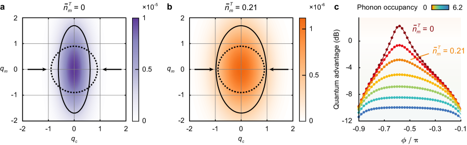
Supplementary Figure 3: Wigner function and quantum advantage. a-b Reconstructed Wigner function of the squeezed state for a pair of canonical quadratures, where the other two quadratures are integrated out. The dashed circles indicate a drop by $1/\mathrm{e}$ of the maximum value. c The theoretical prediction of the quantum advantage versus homodyne angle with different mean phonon occupations. The positive quantum advantage represents sub-SQL sensitivity. The experimental parameters are $G/\kappa=0.1$, $C/C_{\mathrm{SQL}}=0.505$ (ref. Bruch et al. (2019)).

Due to the linearized dynamics and the Gaussian nature of the quantum noise, the steady state of the system finally evolves into a bipartite zero-mean Gaussian state, which is fully characterized by a $4\times 4$ correlation matrix $\mathbf{V}$. Under the stability condition, the steady-state correlation matrix fulfills the Lyapunov equation Barzanjeh et al. (2019):

$$\mathbf{M}\mathbf{V}+\mathbf{V}\mathbf{M}^{\mathrm{T}}=-\mathbf{D},$$ (20)

where matrix $\mathbf{M}$ in a $2\times 2$ block form is given in the main text:

$$\mathbf{M}=\begin{pmatrix}\mathbf{A}&\mathbf{B}\\ \mathbf{B}&\mathbf{C}\\ \end{pmatrix},$$ (21)

and $\mathbf{D}=\mathrm{Diag}\quantity(\sqrt{\kappa},\,\sqrt{\kappa},\,0,\,\sqrt{2\Gamma_{m}})$ is the diffusion matrix, quantifying the stationary noise correlations. Then, the Wigner function well visualizes quantum squeezing via a multivariate normal distribution Barzanjeh et al. (2019):

$$W(\psi)=\frac{\exp\quantity[-\frac{1}{2}\quantity(\psi\mathbf{V}^{-1}\psi^{\dagger})]}{\pi^{2}\sqrt{\operatorname{det}\mathbf{V}}},$$ (22)

where $\psi=\quantity(\delta q_{c},\,\delta p_{c},\,\delta q_{m},\,\delta p_{m})$ is the state vector of the quadrature fluctuations. Supplementary Fig. 3a-b shows the characteristic projections of the reconstructed Wigner function $W(\psi)$. In comparison with the theoretical vacuum state $\mathbf{V}_{\mathrm{vac}}=I/2$ ($I$ is the identity matrix), we achieve cross-quadrature squeezing between optical and mechanical modes below the SQL (Supplementary Fig. 3a). However, as the increase of the temperatures, the effect of quantum squeezing is diminished by the thermal noise (Supplementary Fig. 3b).

In this paper, the quantum advantage is defined as the ratio of the sensitivity enabled by the squeezed light to that acquired from the coherent light Li et al. (2021):

$$\text{quantum advantage}\,($\mathrm{dB}$)=10\lg\sqrt{\frac{\bar{S}_{\mathrm{FF}}^{\mathrm{SQL}}}{\bar{S}_{\mathrm{FF}}^{\phi}}}.$$ (23)

As shown in Supplementary Fig. 3c, the quantum advantage is significant ($>$1\text{\,}\mathrm{dB}$$) only for cryogenic temperatures and can be optimized by tuning the homodyne angle within a certain range.

Supplementary Note 6:  Signal-to-noise ratio and the optimal variance

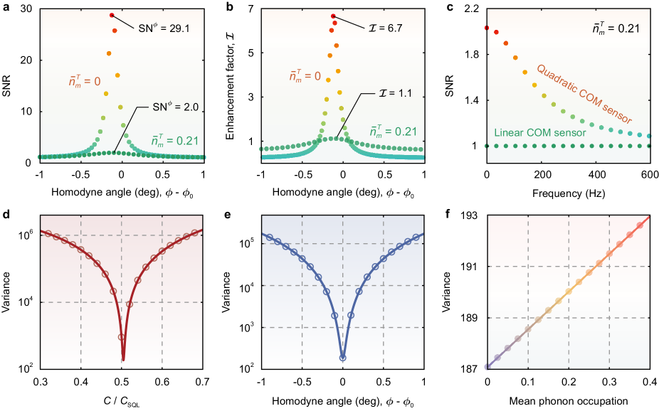
Supplementary Figure 4: Signal-to-noise ratio (SNR) and the optimal variance. a-b SNR for quadratic COM sensors and its enhancement compared with no squeezing regime. The reference phase is chosen as $\phi_{0}=$-97.92\text{\,}\mathrm{\SIUnitSymbolDegree}$$. c Comparison of SNR for linear and quadratic COM sensors without squeezing. d-f The variance of the optimal quadrature. The remaining parameters are $C/C_{\mathrm{SQL}}=0.505$, $G/\kappa=0.246$ (ref. Bruch et al. (2019)).

The performance of the state-of-the-art sensors is commonly quantified by the signal-to-noise ratio (SNR). In our scheme, the spectral density of the signal force is estimated by Sudhir et al. (2017): $\bar{S}_{\mathrm{FF}}^{\mathrm{est},\phi}\quantity[\Omega]=\bar{S}_{\mathrm{FF}}^{\mathrm{sig}}+\bar{S}_{\mathrm{FF}}^{\phi}$, with the SNR recorded as Sudhir et al. (2017)

$$\operatorname{SN}^{\phi}\quantity[\Omega]=\frac{\bar{S}_{\mathrm{FF}}^{\mathrm{est},\phi}}{\bar{S}_{\mathrm{FF}}^{\mathrm{est},\phi}-\bar{S}_{\mathrm{FF}}^{\mathrm{sig}}},$$ (24)

As shown in Supplementary Fig. 4a, the SNR can reach $29.1$ and $2.0$ at the phonon occupations of $0$ and $0.21$, respectively. Besides, we define the enhancement factor of SNR to compare the results with and without squeezing: $\mathcal{I}\quantity[\Omega]=\operatorname{SN}^{\phi}/\operatorname{SN}^{\mathrm{SQL}}$. We find that compared to no squeezing regime, the SNR with squeezing can be improved to a factor of $6.7$ at zero temperature, and reduces to $1.1$ at mean phonon occupations of $0.21$ (Supplementary Fig. 4b). Also, the quadratic COM sensors provide higher SNRs than the linear COM sensors, as shown in Supplementary Fig. 4c. These findings are consistent with the results both in the main text and in the recent experiment Sudhir et al. (2017).

Supplementary Fig. 4d-f characterizes the variance of the generalized rotated field quadrature, which is given by Meng et al. (2020)

$$V_{\mathrm{qq}}^{\phi}\quantity[\Omega]=\int_{-\infty}^{\infty}\Re{\bar{S}_{\mathrm{qq}}^{\phi,\mathrm{out}}}\frac{\differential\Omega}{2\pi},$$ (25)

where the optical output spectrum is expressed as Sudhir et al. (2017): $\bar{S}_{\mathrm{qq}}^{\phi,\mathrm{out}}\quantity[\Omega]=\bar{S}_{\mathrm{qq}}^{\mathrm{out}}\left[\Omega\right]\cos^{2}\phi+\bar{S}_{\mathrm{pp}}^{\mathrm{out}}\left[\Omega\right]\sin^{2}\phi+\bar{S}_{\mathrm{pq}}^{\mathrm{out}}\left[\Omega\right]\sin\left(2\phi\right)$. Such a variance reaches its lowest value when choosing proper cooperativity and homodyne angle, which agrees well with the results in the main text. As expected, we have also confirmed that the fluctuations of the output field increase with the heating of the mechanical bath (Supplementary Fig. 4f).

Supplementary Note 7:  Classical noise

Supplementary Figure 5: Contributions of classical noise. a Prominent examples include thermal noise, laser noise, and other physical environment noise Aggarwal et al. (2020). Such classical hurdles lower the relative contributions from the quantum correlations, hence destroying quantum squeezing. b-c Thermal effect on quantum-limited force sensing. Conventional force sensors are dominated by thermal noise, which masks the contributions of detection uncertainty from the measurements themselves Aggarwal et al. (2020). The role of quantum squeezing becomes remarkable, only when thermal noise has been reduced to the level of vacuum zero-point fluctuations.

Recently there has been a tremendous effort to conduct measurements whose sensitivity is limited by quantum noise. However, it remains a fundamental challenge to reduce the classical noise floor, which in principle creates parallel paths of classical correlations and overwhelm quantum fluctuations, hence setting a limit of the conventional measurements Aggarwal et al. (2020). These classical hurdles includes thermal/laser noise, seismic noise, acoustic noise, and actuator/feedback-injected noise (Supplementary Fig. 5). To evade the dominant noise budget—thermal noise, one should devise and fabricate special mechanical materials and structures, such as metamaterials Beccari et al. and soft-clamped membranes Catalini et al. (2020); Tsaturyan et al. (2017).

Supplementary Note 8:  The role of the nonlinear pump mode

Here, we consider the effect of the fluctuations of the SH mode. For a strong pump field, this mode can be eliminated adiabatically, which yields the effective cavity linewidth or the COM coupling rate, with the effective mechanical resonance frequency:

$$\kappa_{s}^{\mathrm{eff}}=\kappa_{s}+\frac{16\nu^{2}n_{s}}{\kappa_{p}+2\mathrm{i}\Delta^{\prime}},\quad\Omega_{m}^{\mathrm{eff}}=-\frac{16G_{p}^{2}\Delta^{\prime}}{\kappa_{p}^{2}+4\Delta^{\prime 2}},\quad G_{s}^{\pm}=G_{s}\pm\frac{4\nu\alpha_{s}G_{p}\mathrm{e}^{\pm\mathrm{i}\theta}}{\kappa_{p}+2\mathrm{i}\Delta^{\prime}},$$ (26)

where $\Delta=\Delta_{c}-g_{s}\bar{q}_{m}^{2}$, $\Delta^{\prime}=\Delta_{p}-g_{p}\bar{q}_{m}^{2}$, $G_{s}=g_{s}\bar{q}_{m}\sqrt{2n_{s}}$, and $G_{p}=g_{p}\bar{q}_{m}\sqrt{2n_{p}}$. Thus, the optical losses are slightly modified by the SH mode due to the photon up-conversion Peano et al. (2015). The additional COM coupling and the mechanical eigenfrequency indicate the contributions of the photon-phonon coupling for the SH mode Peano et al. (2015). Then, the fluctuations of the SH mode can be neglected under a large detuning ($\Delta^{\prime}\gg G_{p}$) and a small second-order nonlinearity ($\nu\ll G_{p}$) Gan et al. (2019); Peano et al. (2015).

Symbol	Definition	Name	Value	References
$\Omega_{m}$		Mechanical resonance frequency	$2\pi\times$1\text{\,}\mathrm{MHz}$$	Galinskiy et al. (2020)
$Q_{m}$		Mechanical quality factor	$5\text{\times}{10}^{8}$	Galinskiy et al. (2020)
$\bar{n}_{m}^{T}$		Mean phonon occupation	$0.21$	Galinskiy et al. (2020)
$m_{\mathrm{eff}}$		Effective mass	$1\text{\,}\mathrm{ng}$	Galinskiy et al. (2020)
$R$		Membrane reflectivity	0.76	Aggarwal et al. (2020)
$L$		Cavity length	$1\text{\,}\mathrm{mm}$	Rossi et al. (2018)
$\lambda_{p}$		Pump laser wavelength	$780\text{\,}\mathrm{nm}$	Bruch et al. (2019)
$\lambda_{s}$		Signal laser wavelength	$1560\text{\,}\mathrm{nm}$	Bruch et al. (2019)
$\kappa$		Cavity linewidth	$2\pi\times$2.75\text{\,}\mathrm{MHz}$$	Galinskiy et al. (2020)
$Q$	$\left.\Omega_{c}\middle/\kappa\right.$	Optical quality factor	$1.1\text{\times}{10}^{7}$	Galinskiy et al. (2020)
$\eta_{c}$	$\left.\kappa_{\mathrm{ex}}\middle/\kappa\right.$	Cavity outcoupling	$1$	Rossi et al. (2018)
$n_{c}$	$\left.\Omega_{m}\middle/\left(2g_{0}\right)\right.$	Mean photon number for the signal mode	$1.08\text{\times}{10}^{13}$	–
$\Omega$		Fourier frequency	$100\text{\,}\mathrm{Hz}$	McCuller et al. (2020)
$\bar{S}_{\mathrm{FF}}^{\mathrm{sig}}$		Signal force spectrum	$\quantity($1.9\text{\,}\mathrm{zN}$)^{2}$\mathrm{/}\mathrm{Hz}$$	Moser et al. (2014)
$g_{\mathrm{om}}$	$\left.\omega^{\prime\prime}\middle/2\right.$	Quadratic coupling strength	$17.3\text{\,}\mathrm{M}\mathrm{Hz}\mathrm{/}\mathrm{n}\mathrm{m}^{2}$	Paraïso et al. (2015)
$g_{0}$	$g_{\mathrm{om}}x_{\mathrm{zp}}^{2}$	Single-photon COM coupling rate	$0.29\text{\,}\mathrm{\SIUnitSymbolMicro Hz}$	Paraïso et al. (2015)
$C$	$\left.4g^{2}\middle/\left(\kappa\Gamma_{m}\right)\right.$	Multi-photon COM cooperativity	$<0.7C_{\mathrm{SQL}}$	–

Supplementary Table 2: Experimentally accessible parameters. Unless specified otherwise, these parameters apply to all numerical calculations in the text.

Supplementary Note 9:  The validity of the high-temperature limit

Herein, we take high-temperature approximation throughout our numerical calculations. However, under realistic experimental parameters, we note that this limit is valid even at cryogenic temperatures. Specifically, the difference between exact and approximate solutions is near $3.5\%$ for tens of microkelvin temperatures. Moreover, such a approximation will not change the fact that our results are competitive with the state-of-the-art sensors. Thus, we can conclude that it is reasonable to apply the high-temperature limit in the main text.

Supplementary Note 10:  System parameters

In Supplementary Table 2 we collect the main symbols and parameters which have been used in this work.

Supplementary References

References

- Clerk et al. (2010) A. A. Clerk, M. H. Devoret, S. M. Girvin, F. Marquardt, and R. J. Schoelkopf, “Introduction to quantum noise, measurement, and amplification,” Rev. Mod. Phys. 82, 1155–1208 (2010).
- Pirandola et al. (2018) S. Pirandola, B. R. Bardhan, T. Gehring, C. Weedbrook, and S. Lloyd, “Advances in photonic quantum sensing,” Nat. Photonics 12, 724–733 (2018).
- Vermeulen et al. (2021) S. M. Vermeulen et al., “Direct limits for scalar field dark matter from a gravitational-wave detector,” Nature 600, 424–428 (2021).
- Westphal et al. (2021) T. Westphal, H. Hepach, J. Pfaff, and M. Aspelmeyer, “Measurement of gravitational coupling between millimetre-sized masses,” Nature 591, 225–228 (2021).
- Forstner et al. (2012) S. Forstner, S. Prams, J. Knittel, E. D. Van Ooijen, J. D. Swaim, G. I. Harris, A. Szorkovszky, W. P Bowen, and H. Rubinsztein-Dunlop, “Cavity optomechanical magnetometer,” Phys. Rev. Lett. 108, 120801 (2012).
- Krause et al. (2012) A. G. Krause, M. Winger, T. D. Blasius, Q. Lin, and O. Painter, “A high-resolution microchip optomechanical accelerometer,” Nat. Photonics 6, 768 (2012).
- Clark et al. (2016) J. B. Clark, F. Lecocq, R. W. Simmonds, J. Aumentado, and J. D. Teufel, “Observation of strong radiation pressure forces from squeezed light on a mechanical oscillator,” Nat. Phys. 12, 683–687 (2016).
- Wollman et al. (2015) E. E. Wollman, C. U. Lei, A. J. Weinstein, J. Suh, A. Kronwald, F. Marquardt, A. A. Clerk, and K. C. Schwab, “Quantum squeezing of motion in a mechanical resonator,” Science 349, 952–955 (2015).
- Pirkkalainen et al. (2015) J.-M. Pirkkalainen, E. Damskägg, M. Brandt, F. Massel, and M. A. Sillanpää, “Squeezing of quantum noise of motion in a micromechanical resonator,” Phys. Rev. Lett. 115, 243601 (2015).
- Suh et al. (2014) J. Suh, A. J. Weinstein, C. U. Lei, E. E. Wollman, S. K. Steinke, P. Meystre, A. A. Clerk, and K. C. Schwab, “Mechanically detecting and avoiding the quantum fluctuations of a microwave field,” Science 344, 1262–1265 (2014).
- Burd et al. (2019) S. C. Burd, R. Srinivas, J. J. Bollinger, A. C. Wilson, D. J. Wineland, D. Leibfried, D. H. Slichter, and D. T. C. Allcock, “Quantum amplification of mechanical oscillator motion,” Science 364, 1163–1165 (2019).
- Møller et al. (2017) C. B. Møller, R. A. Thomas, G. Vasilakis, E. Zeuthen, Y. Tsaturyan, M. Balabas, K. Jensen, A. Schliesser, K. Hammerer, and E. S. Polzik, “Quantum back-action-evading measurement of motion in a negative mass reference frame,” Nature 547, 191–195 (2017).
- Rossi et al. (2018) M. Rossi, D. Mason, J. Chen, Y. Tsaturyan, and A. Schliesser, “Measurement-based quantum control of mechanical motion,” Nature 563, 53–58 (2018).
- Wilson et al. (2015) D. J. Wilson, V. Sudhir, N. Piro, R. Schilling, A. Ghadimi, and T. J. Kippenberg, “Measurement-based control of a mechanical oscillator at its thermal decoherence rate,” Nature 524, 325–329 (2015).
- Whittle et al. (2021) C. Whittle, E. D. Hall, S. Dwyer, N. Mavalvala, V. Sudhir, R. Abbott, A. Ananyeva, C. Austin, L. Barsotti, J. Betzwieser, et al., “Approaching the motional ground state of a 10-kg object,” Science 372, 1333–1336 (2021).
- Yu et al. (2020) H. Yu et al., “Quantum correlations between light and the kilogram-mass mirrors of LIGO,” Nature 583, 43–47 (2020).
- Aggarwal et al. (2020) N. Aggarwal, T. J. Cullen, J. Cripe, G. D. Cole, R. Lanza, A. Libson, D. Follman, P. Heu, T. Corbitt, and N. Mavalvala, “Room-temperature optomechanical squeezing,” Nat. Phys. 16, 784–788 (2020).
- Cripe et al. (2019) J. Cripe, N. Aggarwal, R. Lanza, A. Libson, R. Singh, P. Heu, D. Follman, G. D. Cole, N. Mavalvala, and T. Corbitt, “Measurement of quantum back action in the audio band at room temperature,” Nature 568, 364–367 (2019).
- Yap et al. (2020) M. J. Yap, J. Cripe, G. L. Mansell, T. G. McRae, R. L. Ward, B. J. J. Slagmolen, P. Heu, D. Follman, G. D. Cole, T. Corbitt, and D. E. McClelland, “Broadband reduction of quantum radiation pressure noise via squeezed light injection,” Nat. Photonics 14, 19–23 (2020).
- Braginsky and Khalili (1996) V. B. Braginsky and F. Y. Khalili, “Quantum nondemolition measurements: the route from toys to tools,” Rev. Mod. Phys. 68, 1 (1996).
- Ockeloen-Korppi et al. (2018) C. F. Ockeloen-Korppi, E. Damskägg, G. S. Paraoanu, F. Massel, and M. A. Sillanpää, “Revealing Hidden Quantum Correlations in an Electromechanical Measurement,” Phys. Rev. Lett. 121, 243601 (2018).
- Ockeloen-Korppi et al. (2017) C. F. Ockeloen-Korppi, E. Damskägg, J.-M. Pirkkalainen, T. T. Heikkilä, F. Massel, and M. A. Sillanpää, “Noiseless Quantum Measurement and Squeezing of Microwave Fields Utilizing Mechanical Vibrations,” Phys. Rev. Lett. 118, 103601 (2017).
- Sudhir et al. (2017) V. Sudhir, R. Schilling, S. A. Fedorov, H. Schutz, D. J. Wilson, and T. J. Kippenberg, “Quantum Correlations of Light from a Room-Temperature Mechanical Oscillator,” Phys. Rev. X 7, 031055 (2017).
- Purdy et al. (2017) T. P. Purdy, K. E. Grutter, K. Srinivasan, and J. M. Taylor, “Quantum correlations from a room-temperature optomechanical cavity,” Science 356, 1265–1268 (2017).
- de Lépinay et al. (2021) L. M. de Lépinay, C. F. Ockeloen-Korppi, M. J. Woolley, and M. A. Sillanpää, “Quantum mechanics–free subsystem with mechanical oscillators,” Science 372, 625–629 (2021).
- Shomroni et al. (2019a) I. Shomroni, A. Youssefi, N. Sauerwein, L. Qiu, P. Seidler, D. Malz, A. Nunnenkamp, and T. J. Kippenberg, “Two-Tone Optomechanical Instability and Its Fundamental Implications for Backaction-Evading Measurements,” Phys. Rev. X 9, 041022 (2019a).
- Shomroni et al. (2019b) I. Shomroni, L. Qiu, D. Malz, A. Nunnenkamp, and T. J. Kippenberg, “Optical backaction-evading measurement of a mechanical oscillator,” Nat. Commun. 10, 2086 (2019b).
- Ockeloen-Korppi et al. (2016) C. F. Ockeloen-Korppi, E. Damskägg, J.-M. Pirkkalainen, A. A. Clerk, M. J. Woolley, and M. A. Sillanpää, “Quantum Backaction Evading Measurement of Collective Mechanical Modes,” Phys. Rev. Lett. 117, 140401 (2016).
- Lecocq et al. (2015) F. Lecocq, J. B. Clark, R. W. Simmonds, J. Aumentado, and J. D. Teufel, “Quantum Nondemolition Measurement of a Nonclassical State of a Massive Object,” Phys. Rev. X 5, 041037 (2015).
- Safavi-Naeini et al. (2013) A. H. Safavi-Naeini, S. Gröblacher, J. T. Hill, J. Chan, M. Aspelmeyer, and O. Painter, “Squeezed light from a silicon micromechanical resonator,” Nature 500, 185–189 (2013).
- Sankey et al. (2010) J. C. Sankey, C. Yang, B. M. Zwickl, A. M. Jayich, and J. G. E. Harris, “Strong and tunable nonlinear optomechanical coupling in a low-loss system,” Nat. Phys. 6, 707–712 (2010).
- Thompson et al. (2008) J. D. Thompson, B. M. Zwickl, A. M. Jayich, F. Marquardt, S. M. Girvin, and J. G. E. Harris, “Strong dispersive coupling of a high-finesse cavity to a micromechanical membrane,” Nature 452, 72–75 (2008).
- Bruch et al. (2019) A. W. Bruch, X. Liu, J. B. Surya, C.-L. Zou, and H. X. Tang, “On-chip microring optical parametric oscillator,” Optica 6, 1361–1366 (2019).
- Brawley et al. (2016) G. A. Brawley, M. R. Vanner, P. E. Larsen, S. Schmid, A. Boisen, and W. P. Bowen, “Nonlinear optomechanical measurement of mechanical motion,” Nat. Commun. 7, 10988 (2016).
- Peano et al. (2015) V. Peano, H. G. L. Schwefel, C. Marquardt, and F. Marquardt, “Intracavity Squeezing Can Enhance Quantum-Limited Optomechanical Position Detection through Deamplification,” Phys. Rev. Lett. 115, 243603 (2015).
- Bullier et al. (2021) N. P. Bullier, A. Pontin, and P. F. Barker, “Quadratic optomechanical cooling of a cavity-levitated nanosphere,” Phys. Rev. Research 3, L032022 (2021).
- Paraïso et al. (2015) T. K. Paraïso, M. Kalaee, L. Zang, H. Pfeifer, F. Marquardt, and O. Painter, “Position-Squared Coupling in a Tunable Photonic Crystal Optomechanical Cavity,” Phys. Rev. X 5, 041024 (2015).
- Purdy et al. (2010) T. P. Purdy, D. W. C. Brooks, T. Botter, N. Brahms, Z.-Y. Ma, and D. M. Stamper-Kurn, “Tunable Cavity Optomechanics with Ultracold Atoms,” Phys. Rev. Lett. 105, 133602 (2010).
- Lee et al. (2015) D. Lee, M. Underwood, D. Mason, A. B. Shkarin, S. W. Hoch, and J. G. E. Harris, “Multimode optomechanical dynamics in a cavity with avoided crossings,” Nat. Commun. 6, 6232 (2015).
- Leijssen et al. (2017) R. Leijssen, G. R. L. Gala, L. Freisem, J. T. Muhonen, and E. Verhagen, “Nonlinear cavity optomechanics with nanomechanical thermal fluctuations,” Nat. Commun. 8, ncomms16024 (2017).
- Ma et al. (2021) X. Ma, J. J. Viennot, S. Kotler, J. D. Teufel, and K. W. Lehnert, “Non-classical energy squeezing of a macroscopic mechanical oscillator,” Nat. Phys. 17, 322–326 (2021).
- Magrini et al. (2021) L. Magrini, P. Rosenzweig, C. Bach, A. Deutschmann-Olek, S. G. Hofer, S. Hong, N. Kiesel, A. Kugi, and M. Aspelmeyer, “Real-time optimal quantum control of mechanical motion at room temperature,” Nature 595, 373–377 (2021).
- Gilmore et al. (2021) K. A. Gilmore et al., “Quantum-enhanced sensing of displacements and electric fields with two-dimensional trapped-ion crystals,” Science 373, 673–678 (2021).
- Bruch et al. (2021) A. W. Bruch, X. Liu, Z. Gong, J. B. Surya, M. Li, C.-L. Zou, and H. X. Tang, “Pockels soliton microcomb,” Nat. Photonics 15, 21–27 (2021).
- Manley et al. (2021) J. Manley, M. D. Chowdhury, D. Grin, S. Singh, and D. J. Wilson, “Searching for vector dark matter with an optomechanical accelerometer,” Phys. Rev. Lett. 126, 061301 (2021).
- Forstner et al. (2020) S. Forstner, M. Zych, S. Basiri-Esfahani, K. E. Khosla, and W. P. Bowen, “Nanomechanical test of quantum linearity,” Optica 7, 1427–1434 (2020).
- Taylor et al. (2013) M. A. Taylor, J. Janousek, V. Daria, J. Knittel, B. Hage, H.-A. Bachor, and W. P. Bowen, “Biological measurement beyond the quantum limit,” Nat. Photonics 7, 229–233 (2013).
- Casacio et al. (2021) C. A. Casacio, L. S. Madsen, A. Terrasson, M. Waleed, K. Barnscheidt, B. Hage, M. A. Taylor, and W. P. Bowen, “Quantum-enhanced nonlinear microscopy,” Nature 594, 201–206 (2021).
- Basiri-Esfahani et al. (2019) S. Basiri-Esfahani, A. Armin, S. Forstner, and W. P. Bowen, “Precision ultrasound sensing on a chip,” Nat. Commun. 10, 132 (2019).
- Gil-Santos et al. (2020) E. Gil-Santos, J. J. Ruz, O. Malvar, I. Favero, A. Lemaître, P. M. Kosaka, S. García-López, M. Calleja, and J. Tamayo, “Optomechanical detection of vibration modes of a single bacterium,” Nat. Nanotechnol. 15, 469–474 (2020).
- Barzanjeh et al. (2015) S. Barzanjeh, S. Guha, C. Weedbrook, D. Vitali, J. H. Shapiro, and S. Pirandola, “Microwave Quantum Illumination,” Phys. Rev. Lett. 114, 080503 (2015).
- Galinskiy et al. (2020) I. Galinskiy, Y. Tsaturyan, M. Parniak, and E. S. Polzik, “Phonon counting thermometry of an ultracoherent membrane resonator near its motional ground state,” Optica 7, 718–725 (2020).
- Catalini et al. (2020) L. Catalini, Y. Tsaturyan, and A. Schliesser, “Soft-Clamped Phononic Dimers for Mechanical Sensing and Transduction,” Phys. Rev. Appl. 14, 014041 (2020).
- Hälg et al. (2021) D. Hälg et al., “Membrane-Based Scanning Force Microscopy,” Phys. Rev. Appl. 15, L021001 (2021).
- Gavartin et al. (2012) E. Gavartin, P. Verlot, and T. J. Kippenberg, “A hybrid on-chip optomechanical transducer for ultrasensitive force measurements,” Nat. Nanotechnol. 7, 509–514 (2012).
- Mason et al. (2019) D. Mason, J. Chen, M. Rossi, Y. Tsaturyan, and A. Schliesser, “Continuous force and displacement measurement below the standard quantum limit,” Nat. Phys. 15, 745–749 (2019).
- Reinhardt et al. (2016) C. Reinhardt, T. Müller, A. Bourassa, and J. C. Sankey, “Ultralow-noise SiN trampoline resonators for sensing and optomechanics,” Phys. Rev. X 6, 021001 (2016).
- Tsaturyan et al. (2017) Y. Tsaturyan, A. Barg, E. S. Polzik, and A. Schliesser, “Ultracoherent nanomechanical resonators via soft clamping and dissipation dilution,” Nat. Nanotechnol. 12, 776–783 (2017).
- Schliesser et al. (2009) A. Schliesser, O. Arcizet, R. Rivière, G. Anetsberger, and T. J. Kippenberg, “Resolved-sideband cooling and position measurement of a micromechanical oscillator close to the Heisenberg uncertainty limit,” Nat. Phys. 5, 509–514 (2009).
- Tao et al. (2014) Y. Tao, J. M. Boss, B. A. Moores, and C. L. Degen, “Single-crystal diamond nanomechanical resonators with quality factors exceeding one million,” Nat. Commun. 5, 3638 (2014).
- Beccari et al. (a) A. Beccari, M. J. Bereyhi, R. Groth, S. A. Fedorov, A. Arabmoheghi, N. J. Engelsen, and T. J. Kippenberg, “Hierarchical tensile structures with ultralow mechanical dissipation,” arXiv:2103.09785 .
- Beccari et al. (b) A. Beccari, D. A. Visani, S. A. Fedorov, M. J. Bereyhi, V. Boureau, N. J. Engelsen, and T. J. Kippenberg, “Strained crystalline nanomechanical resonators with ultralow dissipation,” arXiv:2107.02124 .
- Biercuk et al. (2010) M. J. Biercuk, H. Uys, J. W. Britton, A. P. VanDevender, and J. J. Bollinger, “Ultrasensitive detection of force and displacement using trapped ions,” Nat. Nanotechnol. 5, 646–650 (2010).
- Moser et al. (2013) J. Moser, J. Güttinger, A. Eichler, M. J. Esplandiu, D. E. Liu, M. I. Dykman, and A. Bachtold, “Ultrasensitive force detection with a nanotube mechanical resonator,” Nat. Nanotechnol. 8, 493–496 (2013).
- Rodenburg et al. (2016) B. Rodenburg, L. P. Neukirch, A. N. Vamivakas, and M. Bhattacharya, “Quantum model of cooling and force sensing with an optically trapped nanoparticle,” Optica 3, 318–323 (2016).
- Schreppler et al. (2014) S. Schreppler, N. Spethmann, N. Brahms, T. Botter, M. Barrios, and D. M. Stamper-Kurn, “Optically measuring force near the standard quantum limit,” Science 344, 1486–1489 (2014).
- Weber et al. (2016) P. Weber, J. Güttinger, A. Noury, J. Vergara-Cruz, and A. Bachtold, “Force sensitivity of multilayer graphene optomechanical devices,” Nat. Commun. 7, 12496 (2016).
- De Bonis et al. (2018) S. L. De Bonis, C. Urgell, W. Yang, C. Samanta, A. Noury, J. Vergara-Cruz, Q. Dong, Y. Jin, and A. Bachtold, “Ultrasensitive Displacement Noise Measurement of Carbon Nanotube Mechanical Resonators,” Nano Lett. 18, 5324–5328 (2018).
- Hertzberg et al. (2010) J. B. Hertzberg, T. Rocheleau, T. Ndukum, M. Savva, A. A. Clerk, and K. C. Schwab, “Back-action-evading measurements of nanomechanical motion,” Nat. Phys. 6, 213–217 (2010).
- Gieseler et al. (2013) J. Gieseler, L. Novotny, and R. Quidant, “Thermal nonlinearities in a nanomechanical oscillator,” Nat. Phys. 9, 806–810 (2013).
- (71) S. Dadras et al., “Injection locking of a levitated optomechanical oscillator for precision force sensing,” arXiv:2012.12354 .
- Teufel et al. (2009) J. D. Teufel, T. Donner, M. A. Castellanos-Beltran, J. W. Harlow, and K. W. Lehnert, “Nanomechanical motion measured with an imprecision below that at the standard quantum limit,” Nat. Nanotechnol. 4, 820–823 (2009).
- Gloppe et al. (2014) A. Gloppe, P. Verlot, E. Dupont-Ferrier, A. Siria, P. Poncharal, G. Bachelier, P. Vincent, and O. Arcizet, “Bidimensional nano-optomechanics and topological backaction in a non-conservative radiation force field,” Nat. Nanotechnol. 9, 920–926 (2014).
- Moser et al. (2014) J. Moser, A. Eichler, J. Güttinger, M. I. Dykman, and A. Bachtold, “Nanotube mechanical resonators with quality factors of up to 5 million,” Nat. Nanotechnol. 9, 1007–1011 (2014).
- Liu et al. (2021) Z. Liu, Y. Wei, L. Chen, J. Li, S. Dai, F. Zhou, and M. Feng, “Phonon-Laser Ultrasensitive Force Sensor,” Phys. Rev. Appl. 16, 044007 (2021).
- Fogliano et al. (2021a) F. Fogliano, B. Besga, A. Reigue, P. Heringlake, L. M. de Lépinay, C. Vaneph, J. Reichel, B. Pigeau, and O. Arcizet, “Mapping the Cavity Optomechanical Interaction with Subwavelength-Sized Ultrasensitive Nanomechanical Force Sensors,” Phys. Rev. X 11, 021009 (2021a).
- Tavernarakis et al. (2018) A. Tavernarakis, A. Stavrinadis, A. Nowak, I. Tsioutsios, A. Bachtold, and P. Verlot, “Optomechanics with a hybrid carbon nanotube resonator,” Nat. Commun. 9, 662 (2018).
- Høj et al. (2021) D. Høj, F. Wang, W. Gao, U. B. Hoff, O. Sigmund, and U. L. Andersen, “Ultra-coherent nanomechanical resonators based on inverse design,” Nat. Commun. 12, 5766 (2021).
- Blūms et al. (2018) V. Blūms, M. Piotrowski, M. I. Hussain, B. G. Norton, S. C. Connell, S. Gensemer, M. Lobino, and E. W. Streed, “A single-atom 3D sub-attonewton force sensor,” Sci. Adv. 4, eaao4453 (2018).
- Qin et al. (2021) W. Qin, A. Miranowicz, H. Jing, and F. Nori, “Generating Long-Lived Macroscopically Distinct Superposition States in Atomic Ensembles,” Phys. Rev. Lett. 127, 093602 (2021).
- Purdy et al. (2013a) T. P. Purdy, R. W. Peterson, and C. A. Regal, “Observation of radiation pressure shot noise on a macroscopic object,” Science 339, 801–804 (2013a).
- Purdy et al. (2013b) T. P. Purdy, P.-L. Yu, R. W. Peterson, N. S. Kampel, and C. A. Regal, “Strong optomechanical squeezing of light,” Phys. Rev. X 3, 031012 (2013b).
- Levitan et al. (2016) B. A. Levitan, A. Metelmann, and A. A. Clerk, “Optomechanics with two-phonon driving,” New J. Phys. 18, 093014 (2016).
- Zhao et al. (2020) W. Zhao, S.-D. Zhang, A. Miranowicz, and H. Jing, “Weak-force sensing with squeezed optomechanics,” Sci. China-Phys. Mech. Astron. 63, 224211 (2020).
- Lü et al. (2015) X.-Y. Lü, Y. Wu, J. R. Johansson, H. Jing, J. Zhang, and F. Nori, “Squeezed Optomechanics with Phase-Matched Amplification and Dissipation,” Phys. Rev. Lett. 114, 093602 (2015).
- Qin et al. (2018) W. Qin, A. Miranowicz, P.-B. Li, X.-Y. Lü, J. Q. You, and F. Nori, “Exponentially Enhanced Light-Matter Interaction, Cooperativities, and Steady-State Entanglement Using Parametric Amplification,” Phys. Rev. Lett. 120, 093601 (2018).
- Zhou et al. (2021) F. Zhou, Y. Bao, R. Madugani, D. A. Long, J. J. Gorman, and T. W. LeBrun, “Broadband thermomechanically limited sensing with an optomechanical accelerometer,” Optica 8, 350–356 (2021).
- Forstner et al. (2014) S. Forstner, E. Sheridan, J. Knittel, C. L. Humphreys, G. A. Brawley, H. Rubinsztein-Dunlop, and W. P. Bowen, “Ultrasensitive optomechanical magnetometry,” Adv. Mater. 26, 6348–6353 (2014).
- Li et al. (2018) B.-B. Li, J. Bílek, U. B. Hoff, L. S. Madsen, S. Forstner, V. Prakash, C. Schäfermeier, T. Gehring, W. P. Bowen, and U. L. Andersen, “Quantum enhanced optomechanical magnetometry,” Optica 5, 850–856 (2018).
- Wu et al. (2014) M. Wu, A. C. Hryciw, C. Healey, D. P. Lake, H. Jayakumar, M. R. Freeman, J. P. Davis, and P. E. Barclay, “Dissipative and Dispersive Optomechanics in a Nanocavity Torque Sensor,” Phys. Rev. X 4, 021052 (2014).
- Ghadimi et al. (2018) A. H. Ghadimi, S. A. Fedorov, N. J. Engelsen, M. J. Bereyhi, R. Schilling, D. J. Wilson, and T. J. Kippenberg, “Elastic strain engineering for ultralow mechanical dissipation,” Science 360, 764–768 (2018).
- de Jong et al. (2022) M. H. J. de Jong, J. Li, C. Gärtner, R. A. Norte, and S. Gröblacher, “Coherent mechanical noise cancellation and cooperativity competition in optomechanical arrays,” Optica 9, 170–176 (2022).
- Fogliano et al. (2021b) F. Fogliano et al., “Ultrasensitive nano-optomechanical force sensor operated at dilution temperatures,” Nat. Commun. 12, 4124 (2021b).
- Liu et al. (2016) Z.-P. Liu et al., “Metrology with -Symmetric Cavities: Enhanced Sensitivity near the -Phase Transition,” Phys. Rev. Lett. 117, 110802 (2016).
- Jing et al. (2011) H. Jing, D. S. Goldbaum, L. Buchmann, and P. Meystre, “Quantum Optomechanics of a Bose-Einstein Antiferromagnet,” Phys. Rev. Lett. 106, 223601 (2011).
Acknowledgments
H.J. is supported by the National Natural Science Foundation of China (NSFC, Grants 11935006 and 11774086). Ş.K.Ö. acknowledges support by the Air Force Office of Scientific Research (AFOSR) Multidisciplinary University Research Initiative (MURI) Award No. FA9550-21-1-0202. C.-W.Q. acknowledges the financial support from A*STAR Pharos Program (Grant 15270 00014, with Project R-263-000-B91-305) and Ministry of Education, Singapore (Project R-263-000-D11-114). F.N. is supported in part by NTT Research, Army Research Office (ARO) (Grant W911NF-18-1-0358), Japan Science and Technology Agency (JST) (via the Q-LEAP program and the CREST Grant JPMJCR1676), Japan Society for the Promotion of Science (JSPS) (via the KAKENHI Grant JP20H00134, and the JSPS-RFBR Grant JPJSBP120194828), and the Foundational Questions Institute Fund (FQXi) (Grant FQXi-IAF19-06), a donor-advised fund of the Silicon Valley Community Foundation. Y.-F.J. is supported by the NSFC (Grant 12147156), the China Postdoctoral Science Foundation (2021M701176) and the science and technology innovation Program of Hunan Province (2021RC2078).

References

- Strekalov et al. (2016) D. V. Strekalov, C. Marquardt, A. B. Matsko, H. G. L. Schwefel, and G. Leuchs, “Nonlinear and quantum optics with whispering gallery resonators,” J. Opt. 18, 123002 (2016).
- Zhang et al. (2018) X. Zhang, Q.-T. Cao, Z. Wang, Y.-x. Liu, C.-W. Qiu, L. Yang, Q. Gong, and Y.-F. Xiao, “Symmetry-breaking-induced nonlinear optics at a microcavity surface,” Nat. Photonics 13, 21–24 (2018).
- Bruch et al. (2019) A. W. Bruch, X. Liu, J. B. Surya, C.-L. Zou, and H. X. Tang, “On-chip microring optical parametric oscillator,” Optica 6, 1361–1366 (2019).
- Eddins et al. (2019) A. Eddins, J. M. Kreikebaum, D. M. Toyli, E. M. Levenson-Falk, A. Dove, W. P. Livingston, B. A. Levitan, L. C. G. Govia, A. A. Clerk, and I. Siddiqi, “High-Efficiency Measurement of an Artificial Atom Embedded in a Parametric Amplifier,” Phys. Rev. X 9, 011004 (2019).
- Marty et al. (2021) G. Marty, S. Combrié, F. Raineri, and A. De Rossi, “Photonic crystal optical parametric oscillator,” Nat. Photonics 15, 53–58 (2021).
- Trovatello et al. (2021) C. Trovatello, A. Marini, X. Xu, C. Lee, F. Liu, N. Curreli, C. Manzoni, S. Dal Conte, K. Yao, A. Ciattoni, et al., “Optical parametric amplification by monolayer transition metal dichalcogenides,” Nat. Photonics 15, 6–10 (2021).
- Peano et al. (2015) V. Peano, H. G. L. Schwefel, C. Marquardt, and F. Marquardt, “Intracavity Squeezing Can Enhance Quantum-Limited Optomechanical Position Detection through Deamplification,” Phys. Rev. Lett. 115, 243603 (2015).
- Vahlbruch et al. (2016) H. Vahlbruch, M. Mehmet, K. Danzmann, and R. Schnabel, “Detection of 15 dB Squeezed States of Light and their Application for the Absolute Calibration of Photoelectric Quantum Efficiency,” Phys. Rev. Lett. 117, 110801 (2016).
- Lu et al. (2021a) X. Lu, G. Moille, A. Rao, D. A. Westly, and K. Srinivasan, “Efficient photoinduced second-harmonic generation in silicon nitride photonics,” Nat. Photonics 15, 131–136 (2021a).
- Wang et al. (2021) J.-Q. Wang, Y.-H. Yang, M. Li, X.-X. Hu, J. B. Surya, X.-B. Xu, C.-H. Dong, G.-C. Guo, H. X. Tang, and C.-L. Zou, “Efficient Frequency Conversion in a Degenerate Microresonator,” Phys. Rev. Lett. 126, 133601 (2021).
- Guo et al. (2016) X. Guo, C.-L. Zou, H. Jung, and H. X. Tang, “On-Chip Strong Coupling and Efficient Frequency Conversion between Telecom and Visible Optical Modes,” Phys. Rev. Lett. 117, 123902 (2016).
- Luo et al. (2019) R. Luo, Y. He, H. Liang, M. Li, J. Ling, and Q. Lin, “Optical Parametric Generation in a Lithium Niobate Microring with Modal Phase Matching,” Phys. Rev. Appl. 11, 034026 (2019).
- Xu et al. (2021) Y. Xu, A. A. Sayem, L. Fan, C.-L. Zou, S. Wang, R. Cheng, W. Fu, L. Yang, M. Xu, and H. X. Tang, “Bidirectional interconversion of microwave and light with thin-film lithium niobate,” Nat. Commun. 12, 4453 (2021).
- Lu et al. (2021b) J. Lu, A. A. Sayem, Z. Gong, J. B. Surya, C.-L. Zou, and H. X. Tang, “Ultralow-threshold thin-film lithium niobate optical parametric oscillator,” Optica 8, 539–544 (2021b).
- Lin et al. (2016) J. Lin, Y. Xu, J. Ni, M. Wang, Z. Fang, L. Qiao, W. Fang, and Y. Cheng, “Phase-Matched Second-Harmonic Generation in an On-Chip \chLiNbO3 Microresonator,” Phys. Rev. Appl. 6, 014002 (2016).
- Lake et al. (2016) D. P. Lake, M. Mitchell, H. Jayakumar, L. F. dos Santos, D. Curic, and P. E. Barclay, “Efficient telecom to visible wavelength conversion in doubly resonant gallium phosphide microdisks,” Appl. Phys. Lett. 108, 031109 (2016).
- Fürst et al. (2010) J. U. Fürst, D. V. Strekalov, D. Elser, M. Lassen, U. L. Andersen, C. Marquardt, and G. Leuchs, “Naturally Phase-Matched Second-Harmonic Generation in a Whispering-Gallery-Mode Resonator,” Phys. Rev. Lett. 104, 153901 (2010).
- Ilchenko et al. (2004) V. S. Ilchenko, A. A. Savchenkov, A. B. Matsko, and L. Maleki, “Nonlinear Optics and Crystalline Whispering Gallery Mode Cavities,” Phys. Rev. Lett. 92, 043903 (2004).
- Wang et al. (2018) C. Wang, C. Langrock, A. Marandi, M. Jankowski, M. Zhang, B. Desiatov, M. M. Fejer, and M. Lončar, “Ultrahigh-efficiency wavelength conversion in nanophotonic periodically poled lithium niobate waveguides,” Optica 5, 1438–1441 (2018).
- Mondain et al. (2019) F. Mondain, T. Lunghi, A. Zavatta, E. Gouzien, F. Doutre, M. De Micheli, S. Tanzilli, and V. D’Auria, “Chip-based squeezing at a telecom wavelength,” Photon. Res. 7, A36–A39 (2019).
- Bhattacharya et al. (2008) M. Bhattacharya, H. Uys, and P. Meystre, “Optomechanical trapping and cooling of partially reflective mirrors,” Phys. Rev. A 77, 033819 (2008).
- Sankey et al. (2010) J. C. Sankey, C. Yang, B. M. Zwickl, A. M. Jayich, and J. G. E. Harris, “Strong and tunable nonlinear optomechanical coupling in a low-loss system,” Nat. Phys. 6, 707–712 (2010).
- Thompson et al. (2008) J. D. Thompson, B. M. Zwickl, A. M. Jayich, F. Marquardt, S. M. Girvin, and J. G. E. Harris, “Strong dispersive coupling of a high-finesse cavity to a micromechanical membrane,” Nature 452, 72–75 (2008).
- Paraïso et al. (2015) T. K. Paraïso, M. Kalaee, L. Zang, H. Pfeifer, F. Marquardt, and O. Painter, “Position-Squared Coupling in a Tunable Photonic Crystal Optomechanical Cavity,” Phys. Rev. X 5, 041024 (2015).
- Liao and Nori (2014) J.-Q. Liao and F. Nori, “Single-photon quadratic optomechanics,” Sci. Rep. 4, 6302 (2014).
- Zheng and Li (2021) X. Zheng and B. Li, “Fröhlich condensate of phonons in optomechanical systems,” Phys. Rev. A 104, 043512 (2021).
- Xu et al. (2020) X. Xu, Y. Zhao, H. Wang, H. Jing, and A. Chen, “Quantum nonreciprocality in quadratic optomechanics,” Photon. Res. 8, 143–150 (2020).
- Yap et al. (2020) M. J. Yap, J. Cripe, G. L. Mansell, T. G. McRae, R. L. Ward, B. J. J. Slagmolen, P. Heu, D. Follman, G. D. Cole, T. Corbitt, and D. E. McClelland, “Broadband reduction of quantum radiation pressure noise via squeezed light injection,” Nat. Photonics 14, 19–23 (2020).
- Gavartin et al. (2012) E. Gavartin, P. Verlot, and T. J. Kippenberg, “A hybrid on-chip optomechanical transducer for ultrasensitive force measurements,” Nat. Nanotechnol. 7, 509–514 (2012).
- Lü et al. (2015) X.-Y. Lü, Y. Wu, J. R. Johansson, H. Jing, J. Zhang, and F. Nori, “Squeezed Optomechanics with Phase-Matched Amplification and Dissipation,” Phys. Rev. Lett. 114, 093602 (2015).
- Sudhir et al. (2017) V. Sudhir, R. Schilling, S. A. Fedorov, H. Schutz, D. J. Wilson, and T. J. Kippenberg, “Quantum Correlations of Light from a Room-Temperature Mechanical Oscillator,” Phys. Rev. X 7, 031055 (2017).
- Wimmer et al. (2014) M. H. Wimmer, D. Steinmeyer, K. Hammerer, and M. Heurs, “Coherent cancellation of backaction noise in optomechanical force measurements,” Phys. Rev. A 89, 053836 (2014).
- Xu and Taylor (2014) X. Xu and J. M. Taylor, “Squeezing in a coupled two-mode optomechanical system for force sensing below the standard quantum limit,” Phys. Rev. A 90, 043848 (2014).
- Barzanjeh et al. (2019) S. Barzanjeh, E. S. Redchenko, M. Peruzzo, M. Wulf, D. P. Lewis, G. Arnold, and J. M. Fink, “Stationary entangled radiation from micromechanical motion,” Nature 570, 480–483 (2019).
- Li et al. (2021) F. Li, T. Li, M. O. Scully, and G. S. Agarwal, “Quantum Advantage with Seeded Squeezed Light for Absorption Measurement,” Phys. Rev. Appl. 15, 044030 (2021).
- Meng et al. (2020) C. Meng, G. A. Brawley, J. S. Bennett, M. R. Vanner, and W. P. Bowen, “Mechanical Squeezing via Fast Continuous Measurement,” Phys. Rev. Lett. 125, 043604 (2020).
- Aggarwal et al. (2020) N. Aggarwal, T. J. Cullen, J. Cripe, G. D. Cole, R. Lanza, A. Libson, D. Follman, P. Heu, T. Corbitt, and N. Mavalvala, “Room-temperature optomechanical squeezing,” Nat. Phys. 16, 784–788 (2020).
- (38) A. Beccari, Mohammad J. Bereyhi, R. Groth, S. A. Fedorov, A. Arabmoheghi, N. J. Engelsen, and T. J. Kippenberg, “Hierarchical tensile structures with ultralow mechanical dissipation,” arXiv:2103.09785 .
- Catalini et al. (2020) L. Catalini, Y. Tsaturyan, and A. Schliesser, “Soft-Clamped Phononic Dimers for Mechanical Sensing and Transduction,” Phys. Rev. Appl. 14, 014041 (2020).
- Tsaturyan et al. (2017) Y. Tsaturyan, A. Barg, E. S. Polzik, and A. Schliesser, “Ultracoherent nanomechanical resonators via soft clamping and dissipation dilution,” Nat. Nanotechnol. 12, 776–783 (2017).
- Gan et al. (2019) J.-H. Gan, Y.-C. Liu, C. Lu, X. Wang, M. K. Tey, and L. You, “Intracavity-Squeezed Optomechanical Cooling,” Laser Photonics Rev. 13, 1900120 (2019).
- Galinskiy et al. (2020) I. Galinskiy, Y. Tsaturyan, M. Parniak, and E. S. Polzik, “Phonon counting thermometry of an ultracoherent membrane resonator near its motional ground state,” Optica 7, 718–725 (2020).
- Rossi et al. (2018) M. Rossi, D. Mason, J. Chen, Y. Tsaturyan, and A. Schliesser, “Measurement-based quantum control of mechanical motion,” Nature 563, 53–58 (2018).
- McCuller et al. (2020) L. McCuller et al., “Frequency-Dependent Squeezing for Advanced LIGO,” Phys. Rev. Lett. 124, 171102 (2020).
- Moser et al. (2014) J. Moser, A. Eichler, J. Güttinger, M. I. Dykman, and A. Bachtold, “Nanotube mechanical resonators with quality factors of up to 5 million,” Nat. Nanotechnol. 9, 1007–1011 (2014).