Is first-order relativistic hydrodynamics in general frame stable and causal for arbitrary interaction?

Abstract

We derive a first-order, stable and causal, relativistic hydrodynamic theory from the microscopic kinetic equation using the gradient expansion technique in a general frame. The general frame is introduced from the arbitrary matching conditions for hydrodynamic fields. The interaction is introduced in the relativistic Boltzmann equation through the momentum-dependent relaxation time approximation (MDRTA) with the proposed collision operator that preserves the conservation laws. We demonstrate here for the first time that not only the general frame choice, but also the momentum dependence of microscopic interaction rate, captured through MDRTA, is imperative for producing the essential field corrections that give rise to a causal and stable first-order relativistic theory.

Introduction.$\textendash$ The hydrodynamic theory is an effective coarse-grained formulation of the underlying microscopic dynamics at the long-wavelength limit, that has served for decades as an efficient and accessible tool for a vast range of problems in theoretical physics. However convenient, the relativistic extension of the first-order dissipative Navier-Stokes (NS) formalism introduced by Landau-Lifshitz (LL) LL and Eckart  Eckart , encounters severe issues with instability Hiscock:1983zz ; Hiscock:1985zz ; Hiscock:1987zz and superluminal signal propagation, which pose serious limitation to the practical application of the theory. Later on, second-order Muller-Israel-Stewart (MIS) theory Muller:1967zza ; Israel:1976tn ; Israel:1979wp and some of its extended versions  Muronga:2001zk ; Denicol:2012cn ; Baier:2007ix ; Jaiswal:2013vta ; Grozdanov:2015kqa are introduced to remedy these problems. Recently, a new study has been proposed by Bemfica, Disconzi, Noronha, and Kovtun (BDNK) Bemfica:2017wps ; Bemfica:2019knx ; Bemfica:2020zjp ; Kovtun:2019hdm ; Hoult:2020eho ; Hoult:2021gnb ; Rocha:2022ind for a first-order stable and causal theory by defining the out of equilibrium hydrodynamic variables in a general frame other than LL or Eckart through their postulated constitutive relations that include both time and space gradients.

In this work, we have derived a first-order theory using gradient expansion technique in an arbitrary frame where the explicit expressions of the field redefinition coefficients have been estimated from the underlying microscopic dynamics. The homogeneous part of the out of equilibrium momentum distribution has been extracted from the hydrodynamic matching conditions. The inhomogeneous part obtained from the Boltzmann equation becomes sensitive to the system interactions through its collision term. The relaxation time approximation (RTA) Relax is proven to be a convenient form for linearization of the collision kernel with a wide range of applications (see Ref. Florkowski:2017olj and references therein) and its momentum dependence can be related to the microscopic interaction relevant for the medium under consideration Dusling:2009df . These two facts provide a strong motivation to use momentum dependent relaxation time approximation (MDRTA) in the relativistic transport equation to obtain the inhomogeneous part of the solution  Teaney:2013gca ; Kurkela:2017xis ; Rocha:2021lze ; Rocha:2021zcw ; Mitra:2020gdk ; Mitra:2021owk ; Mitra:2021ubx ; Dash:2021ibx . Here we propose a new collision operator under MDRTA which obeys the fundamental microscopic and macroscopic conservation laws irrespective of particular momentum dependence of RTA or the matching indices. With this formalism, here we have analytically calculated the values of the coefficients in the constitutive relations of hydrodynamic field redefinition from the kinetic theory in a general frame, i.e., for arbitrary matching conditions.

We further analyse the dispersion relation resulting from small perturbations around the hydrostatic equilibrium for this first-order theory to investigate the stability and causality of the system. It is observed that the first-order field correction coefficients responsible for generating causal and stable modes are directly related to the microscopic dynamics of the system. Even in a general frame where the first-order theory is expected to be causal and stable, we find that only non-zero momentum dependence of relaxation time gives rise to the causal and stable modes. The stability and causality conditions critically depend upon the particular momentum dependence of MDRTA. These are the key findings of the current work. To the best of our knowledge, for the first time, a correlation between the interaction dynamics and the causality and stability of a relativistic fluid is being reported.

Throughout the manuscript, we have used natural unit ($\hbar=c=k_{B}=1$) and flat space-time with mostly negative metric $g^{\mu\nu}=\text{diag}\left(1,-1,-1,-1\right)$.

Hydrodynamic field redefinition.$\textendash$ The basic idea is to employ the relativistic Boltzmann transport equation to estimate the out-of-equilibrium one-particle distribution function $f(x,p)$ for general hydrodynamic frame (defined later),

$$p^{\mu}\partial_{\mu}f(x,p)=C[f]=-\cal{L}[\phi]~{}.$$ (1)

Here $p$ is the particle four-momenta and $x$ denotes the space-time variable, $f=f^{(0)}+f^{(0)}(1\pm f^{(0)})\phi$ with $f^{(0)}(=[exp(\frac{p\cdot u}{T}-\frac{\mu}{T})\mp 1]^{-1}$ for Bosons and Fermions respectively) as the equilibrium distribution and $\phi$ is the out of equilibrium deviation; $C[f]$ is the collision integral corresponds to the two-to-two elastic collisions. It is linearized as ${\cal{L}}[\phi]=\int d\Gamma_{p_{1}}d\Gamma_{p^{\prime}}d\Gamma_{p^{\prime}_{1}}f^{(0)}f_{1}^{(0)}(1\pm f^{\prime(0)})(1\pm f_{1}^{\prime(0)})\{\phi+\phi_{1}-\phi^{\prime}-\phi^{\prime}_{1}\}W(p^{\prime}p^{\prime}_{1}|pp_{1})$, with $d\Gamma_{p}=\frac{d^{3}p}{(2\pi)^{3}p^{0}}$ and $W$ is the transition rate that depends on the cross-section of the interactions. In gradient expansion technique $\phi$ is expressed as $\phi=\sum_{r}\phi^{(r)}$, with $\phi^{(r)}$ as the $r^{th}$ order out-of-equilibrium deviation of the distribution function.

In general, $\phi^{(r)}$ can be expressed as a linear combination of $r^{th}$ order field gradients with appropriate tensor coefficients Degroot :

$$\phi^{(r)}=\sum_{l}A^{(r)}_{l}X^{(r)l}+\sum_{m}B_{m}^{(r)\mu}Y^{(r)m}_{\mu}+\sum_{n}C_{n}^{(r)\mu\nu}Z^{(r)n}_{\mu\nu}~{},$$ (2)

with $X^{(r)l},Y^{(r)m}_{\mu}$ and $Z^{(r)n}_{\mu\nu}$ are the $r^{th}$ order scalar, vector and rank-2 tensor gradient corrections of $l,m$, and $n^{th}$ kind respectively. $A_{l}^{(r)},B_{m}^{(r)\mu}$ and $C_{n}^{(r)\mu\nu}$ are the unknown coefficients functions of space-time, particle momentum and the ratio of it’s rest mass to the temperature $z=m/T$. We expand the coefficients in a polynomial basis to extract their values as, $A_{l}^{(r)}=\sum_{s=0}^{\infty}A_{l}^{r,s}(z,x)P_{s}^{(0)},B_{m}^{(r)\mu}=\sum_{s=0}^{\infty}B_{m}^{r,s}(z,x)P_{s}^{(1)}\tilde{p}^{\langle\mu\rangle}$, $C_{n}^{(r)\mu\nu}=\sum_{s=0}^{\infty}C_{n}^{r,s}(z,x)P_{s}^{(2)}\tilde{p}^{\langle\mu}\tilde{p}^{\nu\rangle}$. Inspired from  Dobado:2011qu and being convenient for the current analysis, we employ an orthogonal polynomial basis which are partially orthogonal in the scalar sector. For our case the first two polynomials, $P^{(0)}_{0}=1,~{}P^{(0)}_{1}=\tilde{E}_{p}$ are not orthogonal but all other higher polynomials are chosen to be orthogonal to these two as well as among themselves and monic (in $P^{(n)}_{s}$ the coefficient of maximum power of $\tilde{E}_{p}$, i.e, ${\tilde{E}_{p}}^{s}$ is 1). Concisely they are given by,

$$P^{(0)}_{0}=1~{},~{}~{}P^{(0)}_{1}=\tilde{E}_{p}~{},~{}~{}P^{(1)}_{0}=1~{},~{}~{}P^{(2)}_{0}=1~{},$$ (3)

$$\int dF_{p}(\tilde{E}_{p}/\tau_{R})(\Delta_{\mu\nu}p^{\mu}p^{\nu})^{n}P_{s}^{(n)}P_{r}^{(n)}\sim\delta_{s,r}~{},$$ (4)

with $\tau_{R}$ as the relaxation time of single particle distribution function that will be introduced later with more details. The used notations are, $dF_{p}=d\Gamma_{p}f^{(0)}(1\pm f^{(0)}),~{}\tilde{p}^{\mu}=p^{\mu}/T$, $\tilde{\mu}=\mu/T$, $\tilde{E}_{p}=u_{\mu}p^{\mu}/T,~{}\tilde{p}_{\langle\mu\rangle}=\Delta_{\mu\nu}\tilde{p}^{\nu}$ and $\tilde{p}_{\langle\mu}\tilde{p}_{\nu\rangle}=\Delta_{\mu\nu}^{\alpha\beta}\tilde{p}_{\alpha}\tilde{p}_{\beta}$ with $T,\mu$ and $u^{\mu}$ as the temperature, chemical potential and fluid four velocity of the system at equilibrium and $\Delta^{\mu\nu}=g^{\mu\nu}-u^{\mu}u^{\nu}$.

It is observed that, by the virtue of the collision integral properties ${\cal{L}}[1]=0$ and ${\cal{L}}[p^{\mu}]=0$, that follow from the particle number and energy-momentum conservation respectively, the coefficients $A_{l}^{r,0},A_{l}^{r,1}$ and $B_{m}^{r,0}$ can not be determined from the transport equation (1) and hence they are called the coefficients of the homogeneous solution. The rest of the coefficients $A_{l}^{r,s},B_{m}^{r,s}$ and $C_{n}^{r,s}$ can be estimated from the transport equation and they are called inhomogeneous or interaction solutions. We take the recourse of the matching conditions which are constraints that set the thermodynamic fields, such as temperature, chemical potential, etc., to their equilibrium values even in the presence of dissipation, to extract the coefficients of the homogeneous part of the distribution function. Each such matching conditions produce one out of an infinite number of possible “hydrodynamic frames” Hoult:2021gnb . From the requirement of setting two scalars and one vector homogeneous coefficients from these constraints, we use the following three matching conditions,

$$\int dF_{p}\tilde{E}_{p}^{i}\phi=0,~{}\int dF_{p}\tilde{E}_{p}^{j}\phi=0,~{}\int dF_{p}\tilde{E}_{p}^{k}\tilde{p}^{\langle\mu\rangle}\phi=0,$$ (5)

with $i\neq j$, $i,j,k$ are non-negative integers. We identify the set of matching indices $(1,2,1)$ and $(1,2,0)$ to represent the LL and Eckart frame respectively. Substituting Eq. (2) in Eq. (5), we find the homogeneous part in terms of the interaction part $\phi_{\text{int}}^{(r)}=\sum_{s=2}^{\infty}P_{s}^{(0)}\sum_{l}A^{r,s}_{l}X^{(r)l}+\tilde{p}^{\langle\mu\rangle}\sum_{s=1}^{\infty}P^{(1)}_{s}\sum_{m}B^{r,s}_{m}Y^{(r)m}_{\mu}+\tilde{p}^{\langle\mu}\tilde{p}^{\mu\rangle}\sum_{s=0}^{\infty}P^{(2)}_{s}\sum_{n}C^{r,s}_{n}Z^{(r)n}_{\mu\nu}$ and the matching indices. Using this prescription, the entire out of equilibrium distribution function for any order becomes,

$$\phi^{(r)}=\phi^{(r)}_{\text{int}} -\tilde{E}_{p}\left[\frac{I_{j}}{\mathcal{D}_{i,j}^{1,0}}\int dF_{p}\tilde{E}_{p}^{i}\phi_{\text{int}}^{(r)}+(i\leftrightarrow j)\right]$$

$$-\left[\frac{I_{j+1}}{\mathcal{D}_{i,j}^{0,1}}\int dF_{p}\tilde{E}_{p}^{i}\phi_{\text{int}}^{(r)}+(i\leftrightarrow j)\right]$$

$$-\frac{\tilde{p}_{\langle\nu\rangle}}{J_{k}}\int dF_{p}\tilde{E}_{p}^{k}\tilde{p}^{\langle\nu\rangle}\phi_{\text{int}}^{(r)}~{}.$$ (6)

Here we use the shorthand notation: $\mathcal{D}_{i,j}^{m,n}=I_{i+m}I_{j+n}-I_{i+n}I_{j+m}$ with the properties $\mathcal{D}_{i,j}^{m,n}=-\mathcal{D}_{i,j}^{n,m}$ and $\mathcal{D}_{i,j}^{m,n}=-\mathcal{D}_{j,i}^{m,n}$. The moment integrals are defined as $I_{n}=\int dF_{p}\tilde{E}_{p}^{n},~{}\Delta^{\mu\nu}J_{n}=\int dF_{p}\tilde{p}^{\langle\mu\rangle}\tilde{p}^{\langle\nu\rangle}\tilde{E}_{p}^{n}$. Eq. (6) provides the out-of-equilibrium parts of the two most general hydrodynamic field variables, namely the particle four-flow ($N^{\mu}$) and the energy-momentum tensor ($T^{\mu\nu}$) respectively for the $r^{th}$ order of gradient correction as,

$$\delta N^{(r)\mu}=\int dF_{p}p^{\mu}\phi^{(r)},~{}~{}\delta T^{(r)\mu\nu}=\int dF_{p}p^{\mu}p^{\nu}\phi^{(r)}~{}.$$ (7)

Utilizing Eq. (7), the non-equilibrium correction to the particle number density ($\delta n^{(r)}=u^{\mu}\delta N^{(r)}_{\mu}$), the energy density ($\delta\epsilon^{(r)}=u^{\mu}u^{\nu}\delta T_{\mu\nu}^{(r)}$), pressure ($\delta P^{(r)}=-\frac{1}{3}\Delta^{\mu\nu}\delta T_{\mu\nu}^{(r)}$), energy flux or momentum density ($W^{(r)\alpha}=\Delta^{\alpha}_{\mu}u_{\nu}\delta T^{(r)\mu\nu}$), and the particle flux ($V^{(r)\alpha}=\Delta^{\alpha}_{\mu}\delta N^{(r)\mu}$) can be estimated order-by-order as,

$$\delta n^{(r)} =\int dF_{p}(p^{\mu}u_{\mu})\phi^{(r)}_{\text{int}}+a^{(r)}\frac{\partial n_{0}}{\partial\tilde{\mu}}+u^{\mu}b^{(r)}_{\mu}T\frac{\partial n_{0}}{\partial T},$$ (8)

$$\delta\epsilon^{(r)} =\int dF_{p}(p^{\mu}u_{\mu})^{2}\phi^{(r)}_{\text{int}}+a^{(r)}\frac{\partial\epsilon_{0}}{\partial\tilde{\mu}}+u^{\mu}b^{(r)}_{\mu}T\frac{\partial\epsilon_{0}}{\partial T}~{},$$ (9)

$$\delta P^{(r)} =\frac{1}{3}\int dF_{p}\big{\{}(p^{\mu}u_{\mu})^{2}-m^{2}\big{\}}\phi^{(r)}_{\text{int}}+a^{(r)}\frac{\partial P_{0}}{\partial\tilde{\mu}}$$

$$\hskip 28.45274pt+u^{\mu}b^{(r)}_{\mu}T\frac{\partial P_{0}}{\partial T}~{},$$ (10)

$$W^{(r)\mu} =\int dF_{p}p^{\langle\mu\rangle}(p^{\mu}u_{\mu})\phi^{(r)}_{\text{int}}-(\epsilon_{0}+P_{0})\Delta^{\mu\nu}b^{(r)}_{\nu},$$ (11)

$$V^{(r)\mu} =\int dF_{p}p^{\langle\mu\rangle}\phi^{(r)}_{\text{int}}-n_{0}\Delta^{\mu\nu}b^{(r)}_{\nu}~{}.$$ (12)

Here, $n_{0},\epsilon_{0}$, and $P_{0}$ are the equilibrium values of particle number density, energy density, and pressure, respectively. $a^{(r)}$ and $b^{(r)\mu}$ are the dimensionless momentum independent quantities given by, $a^{(r)}=\frac{I_{i+1}}{\mathcal{D}_{i,j}^{0,1}}\int dF_{p}\tilde{E}_{p}^{j}\phi_{\text{int}}^{(r)}+(i\leftrightarrow j)~{},u^{\mu}b_{\mu}^{(r)}=\frac{I_{i}}{\mathcal{D}_{i,j}^{1,0}}\int dF_{p}\tilde{E}_{p}^{j}\phi_{\text{int}}^{(r)}+(i\leftrightarrow j)~{},\Delta^{\mu\nu}b_{\nu}^{(r)}=-\frac{1}{J_{k}}\int dF_{p}\tilde{E}_{p}^{k}\tilde{p}^{\langle\mu\rangle}\phi_{\text{int}}^{(r)}~{},$ that define the homogeneous part of $\phi$ as, $\phi^{(r)}_{\text{h}}=a^{(r)}+b^{(r)\mu}\tilde{p}_{\mu}$. Adding up the field corrections for all orders, the most general expressions for $N^{\mu}$ and $T^{\mu\nu}$ are given by,

$$N^{\mu}= (n_{0}+\delta n)u^{\mu}+V^{\mu}~{},$$ (13)

$$T^{\mu\nu}= \left(\epsilon_{0}+\delta\epsilon\right)u^{\mu}u^{\nu}-\left(P_{0}+\delta P\right)\Delta^{\mu\nu}$$

$$+\left(W^{\mu}u^{\nu}+W^{\nu}u^{\mu}\right)+\pi^{\mu\nu}~{},$$ (14)

with $\pi^{\mu\nu}$ as the shear stress tensor.

First-order theory with MDRTA.$\textendash$ Up to now, the discussion was completely general, and the results are applicable for any order in the gradient expansion. To provide the explicit expression for the distribution function from Eq. (6), one needs to estimate the interaction part of the distribution function for a specific order. For this purpose, we employ here the momentum-dependent relaxation time approximation (MDRTA) for solving the relativistic transport equation (1) as a dynamical model study. The idea is to replace ${\cal{L}}[\phi]$ in Eq. (1) with the Anderson-Witting type relaxation kernel, but now we generalise the relaxation time to be momentum dependent. For this purpose, we propose here a collision operator under MDRTA in Eq.(1) as the following,

$${\cal{L}}_{\text{MDRTA}}[\phi] =\frac{\left(p\cdot u\right)}{\tau_{R}}f^{(0)}(1\pm f^{(0)})\bigg{[}\phi$$

$$-\frac{\langle\frac{\tilde{E}_{p}}{\tau_{R}}\tilde{E}_{p}^{2}\rangle\langle\frac{\tilde{E}_{p}}{\tau_{R}}\phi\rangle-\langle\frac{\tilde{E}_{p}}{\tau_{R}}\tilde{E}_{p}\rangle\langle\frac{\tilde{E}_{p}}{\tau_{R}}\phi\tilde{E}_{p}\rangle}{\langle\frac{\tilde{E}_{p}}{\tau_{R}}\rangle\langle\frac{\tilde{E}_{p}}{\tau_{R}}\tilde{E}_{p}^{2}\rangle-\langle\frac{\tilde{E}_{p}}{\tau_{R}}\tilde{E}_{p}\rangle^{2}}$$

$$-\tilde{E}_{p}\frac{\langle\frac{\tilde{E}_{p}}{\tau_{R}}\tilde{E}_{p}\rangle\langle\frac{\tilde{E}_{p}}{\tau_{R}}\phi\rangle-\langle\frac{\tilde{E}_{p}}{\tau_{R}}\rangle\langle\frac{\tilde{E}_{p}}{\tau_{R}}\phi\tilde{E}_{p}\rangle}{\langle\frac{\tilde{E}_{p}}{\tau_{R}}\tilde{E}_{p}\rangle^{2}-\langle\frac{\tilde{E}_{p}}{\tau_{R}}\rangle\langle\frac{\tilde{E}_{p}}{\tau_{R}}\tilde{E}_{p}^{2}\rangle}$$

$$-\tilde{p}_{\langle\nu\rangle}\frac{\langle\frac{\tilde{E}_{p}}{\tau_{R}}\phi\tilde{p}^{\langle\nu\rangle}\rangle}{\frac{1}{3}\langle\frac{\tilde{E}_{p}}{\tau_{R}}\tilde{p}^{\langle\mu\rangle}\tilde{p}_{\langle\mu\rangle}\rangle}\bigg{]}~{},$$ (15)

with $\langle\cdots\rangle=\int dF_{p}(\cdots)$. Eq.(15) readily gives ${\cal{L}}_{\text{MDRTA}}[\phi]=0$ if $\phi=a+b(p\cdot u)+c^{\mu}p_{\langle\mu\rangle}$ with $a,b,c^{\mu}$ being arbitrary momentum independent coefficients. It satisfies the self adjoint property as well, $\int d\Gamma_{p}\psi{\cal{L}}_{\text{MDRTA}}[\phi]=\int d\Gamma_{p}\phi{\cal{L}}_{\text{MDRTA}}[\psi]$. These two combinedly give the summation invariant property $\int d\Gamma_{p}\psi{\cal{L}}_{\text{MDRTA}}[\phi]=0$ for $\psi=a+b(p\cdot u)+c^{\mu}p_{\langle\mu\rangle}$ which immediately results in the conservation laws $\partial_{\mu}N^{\mu}=0$ and $\partial_{\mu}T^{\mu\nu}=0$ microscopically. These conservation laws are not needed to be estimated order by order and are treated non-perturbatively. The preservation of particle number and energy-momentum conservation in ${\cal{L}}_{\text{MDRTA}}[\phi]$ is irrespective of the frame indices or particular momentum dependence of $\tau_{R}$. Eq.(15) resembles the novel relaxation time collision operator introduced in Rocha:2021zcw apart from the fact that it uses the polynomial basis given in Eq. (3)-(4). The advantage of using this basis is that the polynomials associated with the homogeneous part of the solution are in form of simple exponents which reduces the computational complexity significantly.

In the current analysis, the momentum dependence of $\tau_{R}$ is expressed as a power law of $\tilde{E}_{p}$ in the comoving frame, with $\tau_{R}^{0}$ as the momentum independent part; the parameter $\Lambda$ specify the power of the scaled energy.

To solve Eq. (1), we adopt a perturbative expansion introduced in Rocha:2022ind . By decomposing the space-time derivative, the left hand side of Eq.(1) gives rise to a number of time and space derivatives over the fundamental thermodynamic quantities $T,\mu$ and $u^{\mu}$. In popular perturbation approaches like Chapman-Enskog method, the time derivatives are replaced by the spatial ones in order to make the left hand side of Eq.(1) orthogonal to zero modes (homogeneous solutions). By the virtue of the collision operator ${\cal{L}}_{\text{MDRTA}}$ given in Eq.(15), the right hand side of Eq. (1) now retains only the interaction part of $\phi$. It singularly excludes the zero modes of the linearized collision operator, i.e, any function proportional to $1$ and $p^{\mu}$ are not present from the momentum basis of the unknown coefficients in Eq.(2). Because of the fact, the left hand side of Eq.(1) is not necessarily needed to be orthogonal to zero modes in order extract the remaining non-zero mode coefficients, which are itself orthogonal to zero modes as well as among themselves. Hence, the covariant time derivatives appearing on the left hand side of Eq.(1) are not required to be exchanged by the spatial gradients. Employing that, the inhomogeneous or interaction part of the first-order out-of-equilibrium distribution function turns out to be,

$$\frac{\phi_{\text{int}}^{(1)}}{\tau_{R}^{0}}=-\tilde{E}_{p}^{\Lambda-1}\bigg{[}\tilde{E}_{p}^{2}\frac{DT}{T}+\tilde{E}_{p}D\tilde{\mu}+\left(\frac{\tilde{E}_{p}^{2}}{3}-\frac{z^{2}}{3}\right)(\partial\cdot u)+$$

$$\tilde{E}_{p}\tilde{p}^{\langle\mu\rangle}\left(\frac{\nabla_{\mu}T}{T}-Du_{\mu}\right)+\tilde{p}^{\langle\mu\rangle}\nabla_{\mu}\tilde{\mu}-\tilde{p}^{\langle\mu}\tilde{p}^{\nu\rangle}\sigma_{\mu\nu}\bigg{]},$$ (16)

where $\sigma_{\mu\nu}=\nabla_{\langle{\mu}}u_{\nu\rangle}$, $D=u^{\mu}\partial_{\mu}$, and $\nabla^{\mu}=\Delta^{\mu\nu}\partial_{\nu}$ are symmetric trace-less shear tensor, temporal and spatial counterparts of the total space-time derivative respectively. Next, we use Eq. (16) in Eq. (6) to construct $\phi^{(1)}$ in order to calculate the first-order field correction coefficients. From Eq.(8)-(12), the first-order thermodynamic field corrections in a general frame and with arbitrary interactions are given by:

$$\delta n^{(1)},\delta\epsilon^{(1)},\delta P^{(1)}=\nu_{1},\varepsilon_{1},\pi_{1}\frac{DT}{T}+\nu_{2},\varepsilon_{2},\pi_{2}\left(\partial\cdot u\right)$$

$$~{}~{}~{}~{}~{}~{}~{}~{}~{}~{}~{}~{}~{}~{}~{}~{}~{}~{}~{}~{}~{}~{}+\nu_{3},\varepsilon_{3},\pi_{3}D\tilde{\mu}~{},$$ (17)

$$W^{(1)\mu},V^{(1)\mu}=\theta_{1},\gamma_{1}\left[\frac{\nabla^{\mu}T}{T}-Du^{\mu}\right]+\theta_{3},\gamma_{3}\nabla^{\mu}\tilde{\mu}.$$ (18)

The explicit expressions of the field correction coefficients turn out to be elaborate and complicated functions of the frame indices $i,j,k$ and the parameter $\Lambda$ of MDRTA. These field corrections along with $\pi^{(1)\mu\nu}=2\eta\sigma^{\mu\nu}$ ($\eta$ is shear viscosity), constitute the first order out of equilibrium $N^{\mu}$ and $T^{\mu\nu}$ from Eq. (13) and Eq. (14), respectively.

So, here we end up with 14 field correction coefficients ($\nu_{1,2,3},\epsilon_{1,2,3},\pi_{1,2,3},\theta_{1,3},\gamma_{1,3}$ and $\eta$). It was shown in Kovtun:2019hdm ; Hoult:2021gnb that not all coefficients are invariant under the first-order field redefinition (due to the arbitrariness in the definition of temperature, fluid four-velocity and chemical potential for out-of equilibrium case). We checked that our coefficients satisfy the combinations $f_{i}=\pi_{i}-\varepsilon_{i}\left(\frac{\partial P_{0}}{\partial\epsilon_{0}}\right)_{n_{0}}-\nu_{i}\left(\frac{\partial P_{0}}{\partial n_{0}}\right)_{\epsilon_{0}}$ and $l_{i}=\gamma_{i}-\frac{n_{0}}{\epsilon_{0}+P_{0}}\theta_{i}$ to be frame invariant (i.e., independent of the indices $i,j,k$), which further reduce to the physical transport coefficients; bulk viscosity $\zeta=-f_{2}+\left(\frac{\partial P_{0}}{\partial\epsilon_{0}}\right)_{n_{0}}f_{1}+\frac{1}{T}\left(\frac{\partial P_{0}}{\partial n_{0}}\right)_{\epsilon_{0}}f_{3}$, and charge conductivity $k_{n}=l_{3}-\frac{n_{0}T}{(\epsilon_{0}+P_{0})}l_{1}$. The detailed expressions of $\zeta$ and $k_{n}$ with MDRTA are given in Mitra:2021owk . The corrections further reveal that, the LL and Eckart limit of the scalar indices ($i=1,j=2$ or vice versa) give $\delta n^{(1)}=0,\delta\epsilon^{(1)}=0$ (such that $\zeta$ is entirety taken up by the pressure correction), where for the vector index, LL limit ($k=1$) gives $W^{(1)\mu}=0$ and Eckart limit ($k=0$) gives $V^{(1)\mu}=0$. Most significantly, we found that for the momentum independent relaxation time (i.e., for $\Lambda$=0), all the correction coefficients associated with the first-order time derivatives $(\nu_{1},\nu_{3},\varepsilon_{1},\varepsilon_{3},\pi_{1},\pi_{3},\theta_{1},\gamma_{1})$ in Eqs. (17)-(18) identically vanish for all hydrodynamic frame conditions (irrespective of $i,j,k$ values) which will be shown later to have crucial implications on the causality and stability of the theory.

Stability and causality analysis.$\textendash$ Here we investigate the causality and stability of the theory by linearizing the conservation equations for small perturbations of fluid variables around the hydrostatic equilibrium in the local rest frame, $\epsilon(t,x)=\epsilon_{0}+\delta\epsilon(t,x),~{}n=n_{0}+\delta n(t,x),,P(t,x)=P_{0}+\delta P(t,x),~{}u^{\mu}(t,x)=(1,\vec{0})+\delta u^{\mu}(t,x)$. In linear approximation, $\delta u^{\mu}$ has only spatial components to retain the normalization condition. For convenience, these fluctuations are further expressed in their plane wave solutions via a Fourier transformation $\delta\psi(t,x)\rightarrow e^{i(\omega t-kx)}\delta\psi(\omega,k)$, with wave 4-vector $k^{\mu}=(\omega,k,0,0)$. The resulting dispersion relation for transverse or shear channel is,

$$(i\omega)^{2}+i\omega\frac{(\epsilon_{0}+P_{0})}{\theta}+\frac{\eta}{\theta}k^{2}=0~{},$$ (19)

where we define $\theta=-\theta_{1}$. At small $k$ limit, the obtained modes are, $\omega^{T}_{1}=i\frac{\eta}{(\epsilon_{0}+P_{0})}k^{2}+{\cal{O}}(k^{4})$ and $\omega^{T}_{2}=i\frac{(\epsilon_{0}+P_{0})}{\theta}+{\cal{O}}(k^{2})$. Both the modes are non-propagating, where $\omega^{T}_{1}$ is a hydrodynamic mode (vanishes at $k=0$) and $\omega^{T}_{2}$ is a non-hydro mode. $\omega^{T}_{1}$ is the conventional shear mode of NS theory. At small $k$ the stability is guaranteed if $\theta>0$, because in that case the imaginary part of $\omega_{2}^{T}$ is positive definite and gives rise to exponentially decaying perturbations. At large $k$, the modes come out to be $\omega^{T}_{1,2}=\pm\sqrt{\eta/\theta}~{}k+i\frac{(\epsilon_{0}+P_{0})}{2\theta}+{\cal{O}}(\frac{1}{k})$. These are propagating modes where causality holds for $\theta>\eta$, which also guarantees the stability condition. $\theta_{1}$ plays a crucial role in stability and causality of the shear channel. From Eq. (18) the explicit expression of $\theta_{1}$ turns out to be,

$$\theta_{1}=-\tau_{R}^{0}T^{2}\left(J_{\Lambda+1}+\frac{\epsilon_{0}+P_{0}}{T^{2}}\frac{J_{k+\Lambda}}{J_{k}}\right)~{}.$$ (20)

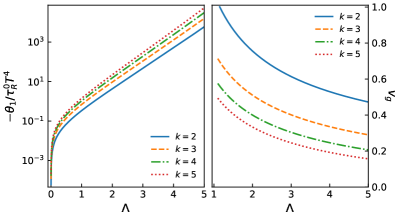
Figure 1: $\theta_{1}$ and $v_{g}$ as a function of $\Lambda$ in general frames

We can see, $\theta_{1}=0$ for both $k=1$ (LL frame) with any interaction or $\Lambda=0$ (momentum independent RTA) for any general frame. This will give rise to superluminal velocities in the shear channel. In Fig. (1), left panel shows $\theta(=-\theta_{1})$ scaled by $\tau_{R}^{0}$ as a function of $\Lambda$ for different vector matching indices $k$. $\theta$ is always positive for $\Lambda>0$. The right panel shows the group velocity $v_{g}=\sqrt{\eta/\theta}$ which obeys causality for $\Lambda>1$, where $\eta=\tau_{R}^{0}T^{2}K_{\Lambda-1}/2$ with $\Delta^{\alpha\beta\mu\nu}K_{n}=\int dF_{p}\tilde{p}^{\langle\mu}\tilde{p}^{\nu\rangle}\tilde{p}^{\langle\alpha}\tilde{p}^{\beta\rangle}\tilde{E}_{p}^{n}~{}$. We also see that, larger values of $k$ and $\Lambda$ reduce group velocity. So, even in a general frame, the choice of $\Lambda$ crucially decides the stability and causality of the shear channel. Throughout the numerical analysis, the parameters have been set to, $T=300$ MeV, $m=300$ MeV.

For longitudinal or sound mode, the dispersion relation turns out to be a sixth order polynomial,

$$(i\omega)^{6}A_{6}+(i\omega)^{5}A_{5}+(i\omega)^{4}A_{4}+(i\omega)^{3}A_{3}$$

$$+(i\omega)^{2}A_{2}+(i\omega)A_{1}+A_{0}=0~{},$$ (21)

with $A_{4}=A_{4}^{0}+A_{4}^{2}k^{2},A_{3}=A_{3}^{0}+A_{3}^{2}k^{2},A_{2}=A_{2}^{2}k^{2}+A_{2}^{4}k^{4},A_{1}=A_{1}^{2}k^{2}+A_{1}^{4}k^{4},A_{0}=A_{0}^{4}k^{4}+A_{0}^{6}k^{6}$. Eq. (21) agrees with result obtained in Taghinavaz:2020axp , where the coefficient $A$’s are functions of $\nu_{1,2,3},\varepsilon_{1,2,3},\pi_{1,2,3},\theta_{1,3},\gamma_{1,3}$ defined earlier (the detailed analysis will be reported elsewhere). Eq. (21) cannot be solved analytically and hence we present results for $k\rightarrow 0$ limit. At this limit, Eq. (21) gives three hydrodynamic modes as, $\omega_{6}^{L}=i\hat{h}^{2}\frac{k_{n}T}{(\epsilon_{0}+P_{0})}k^{2}$ and $\omega_{4,5}^{L}=\pm c_{s}k+i\frac{\Gamma_{s}}{2}k^{2}+{\cal{O}}(k^{3})$, with scaled enthalpy per particle $\hat{h}=(\epsilon_{0}+P_{0})/n_{0}T$, velocity of sound squared $c_{s}^{2}=\big{(}\frac{\partial P_{0}}{\partial\epsilon_{0}}\big{)}_{n_{0}}+\frac{1}{\hat{h}}\frac{1}{T}\big{(}\frac{\partial P_{0}}{\partial n_{0}}\big{)}_{\epsilon_{0}}$ and sound attenuation coefficients $\Gamma_{s}=\left[\frac{4}{3}\eta+\zeta+\frac{k_{n}T}{c_{s}^{2}}\big{(}\frac{1}{T}\frac{\partial P_{0}}{\partial n_{0}}\big{)}^{2}_{\epsilon_{0}}\right]/(\epsilon_{0}+P_{0})$. $\omega_{6}^{L}$ and $\omega_{4,5}^{L}$ are the conventional heat-diffusion and sound modes of the NS theory respectively.

The remaining non-hydro modes are given by,

$$(i\omega^{L})^{3}A_{6}+(i\omega^{L})^{2}A_{5}+(i\omega^{L})A^{0}_{4}+A^{0}_{3}=0~{}.$$ (22)

Using Routh-Hurwitz criteria, we find the following conditions for stability of the non-hydro modes,

$$A_{6}>0~{},~{}A_{5}>0~{},~{}A_{3}^{0}>0~{},$$ (23)

$$B_{2}=(A_{4}^{0}A_{5}-A_{3}^{0}A_{6})/A_{5}>0~{}.$$ (24)

Among these coefficients, $A_{3}^{0}=n_{0}(\epsilon_{0}+P_{0})$ is always positive. The remaining coefficients are given by,

$$A_{6} =\frac{\theta_{1}}{(\epsilon_{0}+P_{0})}\hat{h}c_{s}^{2}(\nu_{1}\epsilon_{3}-\nu_{3}\epsilon_{1})~{},$$ (25)

$$A_{5} =\hat{h}c_{s}^{2}(\nu_{3}\epsilon_{1}-\nu_{1}\epsilon_{3})$$

$$-\theta_{1}\left[(\nu_{1}f+\nu_{3}c)+\frac{1}{\hat{h}T}(\epsilon_{1}g+\epsilon_{3}d)\right]~{},$$ (26)

$$A_{4}^{0} =(\epsilon_{0}+P_{0})(\nu_{1}f+\nu_{3}c)+n_{0}(\epsilon_{1}c+\epsilon_{3}d-\theta_{1})~{}.$$ (27)

with, $c=J_{0}I_{3}/(I_{2}^{2}-I_{1}I_{3})~{},~{}d=-J_{1}I_{2}/(I_{2}^{2}-I_{1}I_{3})~{},~{}f=-J_{0}I_{2}/(I_{2}^{2}-I_{1}I_{3})~{},~{}g=J_{1}I_{1}/(I_{2}^{2}-I_{1}I_{3})$.

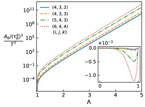
Figure 2: $A_{6}$ as a function of $\Lambda$ in general frames

The concerned field correction coefficients are given by,

$$\varepsilon_{1}=\tau_{R}^{0}\left[\frac{\partial\epsilon_{0}}{\partial\tilde{\mu}}\frac{{\cal{D}}_{i,j}^{\Lambda+1,1}}{{\cal{D}}_{i,j}^{0,1}}+T\frac{\partial\epsilon_{0}}{\partial T}\frac{{\cal{D}}_{i,j}^{\Lambda+1,0}}{{\cal{D}}_{i,j}^{1,0}}-T^{2}I_{\Lambda+3}\right],$$ (28)

$$\varepsilon_{3}=\tau_{R}^{0}\left[\frac{\partial\epsilon_{0}}{\partial\tilde{\mu}}\frac{{\cal{D}}_{i,j}^{\Lambda,1}}{{\cal{D}}_{i,j}^{0,1}}+T\frac{\partial\epsilon_{0}}{\partial T}\frac{{\cal{D}}_{i,j}^{\Lambda,0}}{{\cal{D}}_{i,j}^{1,0}}-T^{2}I_{\Lambda+2}\right]~{},$$ (29)

$$\nu_{1}=\tau_{R}^{0}\left[\frac{\partial n_{0}}{\partial\tilde{\mu}}\frac{{\cal{D}}_{i,j}^{\Lambda+1,1}}{{\cal{D}}_{i,j}^{0,1}}+T\frac{\partial n_{0}}{\partial T}\frac{{\cal{D}}_{i,j}^{\Lambda+1,0}}{{\cal{D}}_{i,j}^{1,0}}-TI_{\Lambda+2}\right]~{},$$ (30)

$$\nu_{3}=\tau_{R}^{0}\left[\frac{\partial n_{0}}{\partial\tilde{\mu}}\frac{{\cal{D}}_{i,j}^{\Lambda,1}}{{\cal{D}}_{i,j}^{0,1}}+T\frac{\partial n_{0}}{\partial T}\frac{{\cal{D}}_{i,j}^{\Lambda,0}}{{\cal{D}}_{i,j}^{1,0}}-TI_{\Lambda+1}\right]~{}.$$ (31)

The coefficients $\nu_{1},\varepsilon_{1}$ vanish both for $i=1,j=2$ (LL+Eckart) $\forall\Lambda$ and also at $\Lambda=0$ for all frame choices. $\nu_{3},\varepsilon_{3}$ obey the same but also vanish for $\Lambda=1$ at all frames. The coefficients make $A_{5}$ and $A_{4}^{0}$ vanish for $\Lambda=0$ and $A_{6}$ vanish for both $\Lambda=0$ and $1$ at any frame.

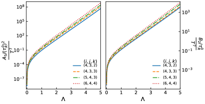
Figure 3: $A_{5}$ and $B_{2}$ as a function of $\Lambda$ in general frames

From Fig. (2) we can see that $A_{6}$ becomes positive for $\Lambda>1$, but it becomes negative for the region $\Lambda$= 0 to 1 excluding the end points. This is shown in the inset of Fig. (2), where we can see that in this region higher values of the frame indices make the situation worse with larger negative values of $A_{6}$, resulting in more increased instability. This is the essence of the current work. In short, we conclude that a general frame and the nature of underlying interactions are both crucial for the stability and causality of a first-order theory. Fig. (3) shows the dependency of $A_{5}$ and $B_{2}$ on $\Lambda$ for different frames, which turns out to be positive for general frames and $\Lambda>0$.

Conclusion. $\textendash$ In this work, a first-order, relativistic stable and causal hydrodynamic theory has been derived in a general frame from the Boltzmann transport equation, where the system interactions are introduced via the microscopic particle momenta captured through $\tau_{R}$ and an appropriate collision operator ${\cal{L}}_{\text{MDRTA}}$. We have shown that in order to hold stability and causality at first-order theories, besides a general frame, the system interactions need to be carefully taken into account. The conventional momentum independent RTA leads to acausality by diverging the shear modes even in a general frame. The momentum dependence employed through MDRTA is shown to subtly control the stability and causality of the theory in a general frame.

We believe that this correlation between system dynamics (microscopic interactions) and relativistic hydrodynamics (macroscopic frame variables), along with the precise estimation of causality and stability conditions, makes the current work an acceptable first-order hydrodynamic theory, ready for practical applications.

Acknowledgements.$\textendash$ R.B. and V.R. acknowledge financial support from the DST Inspire faculty research grant (IFA-16-PH-167), India. S.M. acknowledges funding support from DNAP, TIFR, India.

References

(1)
L.D. Landau and E.M. Lifshitz, Fluid Mechanics (Elsevier, Amsterdam,1987).
(2)
C. Eckart, Phys. Rev. 58 (1940)919.
(3)
W. A. Hiscock and L. Lindblom,
Annals Phys. 151 (1983), 466-496.
(4)
W. A. Hiscock and L. Lindblom,
Phys. Rev. D 31 (1985), 725-733.
(5)
W. A. Hiscock and L. Lindblom,
Phys. Rev. D 35 (1987), 3723-3732.
(6)
I. Muller,
Z. Phys. 198 (1967), 329-344
(7)
W. Israel,
Annals Phys. 100 (1976), 310-331
(8)
W. Israel and J. M. Stewart,
Annals Phys. 118 (1979), 341-372
(9)
A. Muronga,
Phys. Rev. Lett. 88 (2002), 062302.
(10)
G. S. Denicol, H. Niemi, E. Molnar and D. H. Rischke,
Phys. Rev. D 85 (2012), 114047.
(11)
R. Baier, P. Romatschke, D. T. Son, A. O. Starinets and M. A. Stephanov,
JHEP 04 (2008), 100.
(12)
A. Jaiswal,
Phys. Rev. C 87 (2013) no.5, 051901,
A. Jaiswal,
Phys. Rev. C 88 (2013), 021903.
(13)
S. Grozdanov and N. Kaplis,
Phys. Rev. D 93 (2016) no.6, 066012.
(14)
F. S. Bemfica, M. M. Disconzi and J. Noronha,
Phys. Rev. D 98 (2018) no.10, 104064.
(15)
F. S. Bemfica, M. M. Disconzi and J. Noronha,
Phys. Rev. D 100 (2019) no.10, 104020.
(16)
F. S. Bemfica, M. M. Disconzi and J. Noronha,
[arXiv:2009.11388 [gr-qc]].
(17)
P. Kovtun,
JHEP 10 (2019), 034.
(18)
R. E. Hoult and P. Kovtun,
JHEP 06 (2020), 067.
(19)
R. E. Hoult and P. Kovtun,
[arXiv:2112.14042 [hep-th]].
(20)
G. S. Rocha, G. S. Denicol and J. Noronha,
[arXiv:2205.00078 [nucl-th]].
(21)
J. Anderson and H. Witting,
Physica 74, 466 (1974).
(22)
W. Florkowski, M. P. Heller and M. Spalinski,
Rept. Prog. Phys. 81, no.4, 046001 (2018).
(23)
K. Dusling, G. D. Moore and D. Teaney,
Phys. Rev. C 81 (2010), 034907.
(24)
D. Teaney and L. Yan,
Phys. Rev. C 89 (2014) no.1, 014901.
(25)
A. Kurkela and U. A. Wiedemann,
Eur. Phys. J. C 79 (2019) no.9, 776.
(26)
G. S. Rocha, G. S. Denicol and J. Noronha,
Phys. Rev. Lett. 127 (2021) no.4, 042301.
(27)
G. S. Rocha and G. S. Denicol,
Phys. Rev. D 104 (2021) no.9, 096016.
(28)
S. Mitra,
Phys. Rev. C 103 (2021) no.1, 014905.
(29)
S. Mitra,
Phys. Rev. C 105 (2022) no.1, 014902.
(30)
S. Mitra,
[arXiv:2106.08510 [nucl-th]].
(31)
D. Dash, S. Bhadury, S. Jaiswal and A. Jaiswal,
[arXiv:2112.14581 [nucl-th]].
(32)
S. R. De Groot, W. A. Van Leeuwen and C. G. Van Weert,
Relativistic Kinetic Theory, Principles And Applications
(North-holland, Amsterdam, 1980).
(33)
A. Dobado, F. J. Llanes-Estrada and J. M. Torres-Rincon,
Phys. Lett. B 702 (2011), 43-48.