Where Is My Training Bottleneck?
Hidden Trade-Offs in Deep Learning Preprocessing Pipelines

Abstract.

Preprocessing pipelines in deep learning aim to provide sufficient data throughput to keep the training processes busy. Maximizing resource utilization is becoming more challenging as the throughput of training processes increases with hardware innovations (e.g., faster GPUs, TPUs, and inter-connects) and advanced parallelization techniques that yield better scalability. At the same time, the amount of training data needed in order to train increasingly complex models is growing. As a consequence of this development, data preprocessing and provisioning are becoming a severe bottleneck in end-to-end deep learning pipelines.

In this paper, we provide an in-depth analysis of data preprocessing pipelines from four different machine learning domains. We introduce a new perspective on efficiently preparing datasets for end-to-end deep learning pipelines and extract individual trade-offs to optimize throughput, preprocessing time, and storage consumption. Additionally, we provide an open-source profiling library that can automatically decide on a suitable preprocessing strategy to maximize throughput. By applying our generated insights to real-world use-cases, we obtain an increased throughput of 3$\times$ to 13$\times$ compared to an untuned system while keeping the pipeline functionally identical. These findings show the enormous potential of data pipeline tuning.

1. Introduction

Deep learning (DL) models are used in multiple areas, ranging from e-mail spam filtering (Blanzieri and Bryl, 2008) in natural language processing (NLP) to image segmentation tasks for autonomous driving (He et al., 2017) in computer vision (CV). The improvement of these models is not only based on more advanced architectures or algorithms (Vinyals et al., 2015; Szegedy et al., 2015; Lai et al., 2015), but also on increased quality and quantity of training data (Krizhevsky et al., 2012b; Deng et al., 2009; Lin et al., 2014; Everingham and Winn, 2011; Szegedy et al., 2015). Having more training data usually proves to be beneficial to the model performance (Banko and Brill, 2001).

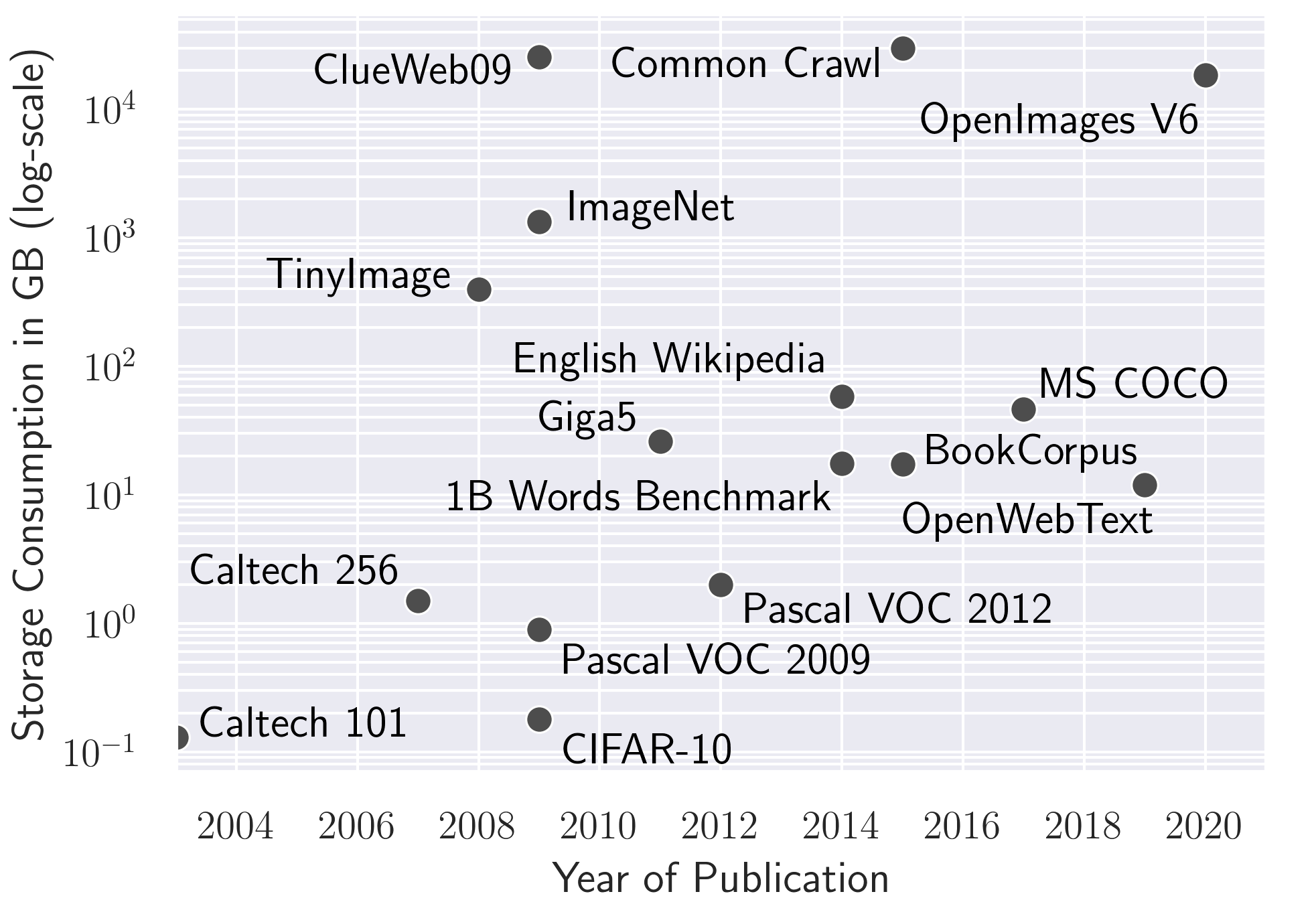
Figure 1. Storage consumption of real-world CV and NLP datasets over time on a logarithmic scale. CV: (Fei-Fei et al., 2004; Gregory et al., 2007; Torralba et al., 2008; Deng et al., 2009; Everingham et al., 2009; Everingham and Winn, 2011; Krizhevsky et al., 2012a; Lin et al., 2014; Krasin et al., 2017), NLP: (Callan et al., 2009; Parker et al., 2011; Chelba et al., 2013; Wikipedia, 2014; Zhu et al., 2015; Common Crawl Foundation, 2012; Aaron Gokaslan, 2019).

The process to train a DL model consists of repeatedly iterating over the entire training dataset, measuring up to hundreds of iterations depending on the task at hand and the model complexity (Peters et al., 2018; He et al., 2016; Szegedy et al., 2016; Radford et al., 2018). Popular datasets show exponential storage consumption increase over time (Fig. 1), which makes data preprocessing harder, as local processing is not viable anymore due to memory limitations. Both distributed storage solutions (Weil et al., 2006) as well as distributed processing (Gabriel et al., 2004; Vishnu et al., 2016; Apache, 2021; Zaharia et al., 2010; Mayer and Jacobsen, 2020) can lead to new difficulties with network I/O and latency, which makes data preprocessing an integral part of the end-to-end DL pipeline. A Google study on their cluster fleet showed that the preprocessing pipeline takes more than a third of the total preprocessing time for 20% of their jobs (Murray et al., 2021).

Optimizing the model training is an active research topic that focuses on decreasing the total training time and increasing the data ingestion rate of the training process. There are many methods on training performance optimization and model optimization for both single GPU (Micikevicius et al., 2018; Vanholder, 2016; Han et al., 2015) and multi-GPU setups (Jäger et al., 2018; Sergeev and Del Balso, 2018; Jia et al., 2019; Ren, [n. d.]) which allow for horizontal scaling with more hardware (NVIDIA, 2020). Recent hardware innovations help with improved model performance (cf. Fig. 3). Therefore, it is essential to optimize preprocessing pipelines to keep up with the training process speed.

The preprocessing part of a DL pipeline consists of multiple successive data transformation steps applied to the initial dataset until the final data representation matches the model input dimensions. This transformation can be performed once before the training or in every iteration while the training is happening. For example, CV pipelines from DL models that established new landmarks at their respective times (Krizhevsky et al., 2012c; Zeiler and Fergus, 2014; Simonyan and Zisserman, 2015; He et al., 2016; Szegedy et al., 2016) follow a common pattern of preprocessing steps: read the image from a storage device, decode it into an RGB matrix and resize the image to fit the model input dimensions. These steps can be followed by data augmentation, e.g., pixel-centering, random-cropping or a rotation, depending on the particular use-case. Preprocessing the full dataset once before training is viable if one wants to avoid the processing overhead in every iteration.

However, the final data representation and the storage device can negatively affect the preprocessing throughput. The training process’s data ingestion can be throttled by I/O bottlenecks when loading the preprocessed data. The storage consumption typically increases at later preprocessing steps, as the corresponding data representations often store data inefficiently to facilitate processing (e.g., JPG (Wallace, 1992) vs. an RBG matrix). This additional storage consumption can be a determining factor that slows down the final throughput. The file system, storage device, and the data loader from the DL framework may not be able to read the data fast enough (cf. Section 4).

We propose a new, more flexible way to look at DL preprocessing pipelines, where the decision for each preprocessing step to apply it once or in every iteration can be made freely based on quantifiable trade-offs. Such quantification can be provided by profiling.

Figure 2. CV preprocessing pipeline

To motivate this new view on preprocessing pipelines, we performed experiments using different configurations of a CV pipeline (Fig. 2) . Performing all preprocessing steps at once increases the throughput by $5.4\times$ compared to at every iteration (Tab. 1). However, this increases storage consumption by more than $10\times$. In contrast, preprocessing the dataset once just until the resize step results in a $16.7\times$ throughput increase while increasing the storage consumption only by $3.4\times$ compared to processing all steps at every iteration.

Preprocessing strategy	Throughput in $\frac{samples}{s}$	Storage Consumption in GB
all steps at every iteration	107	146
all steps once	576	1535
until resize step, once	1789	494

Table 1. Trade-offs for the CV pipeline at different preprocessing strategies.

When comparing the data processing rate of a popular CV model, ResNet-50, to the different preprocessing strategies on state-of-the-art GPUs, we see that stalls on the A10, A30, and V100 can be prevented by using the optimal strategy (Fig.  3). In multi-node training setups and when using specialized hardware (TPUs), increasing preprocessing throughput demands becomes even more evident.

The idea of opening up the preprocessing pipeline and the resulting trade-offs have not been explored yet in a comprehensive fashion. This void prevents ML practitioners from optimizing their end-to-end DL pipelines. They lack guidance in how to do that, as well as tooling support to automate such optimizations.

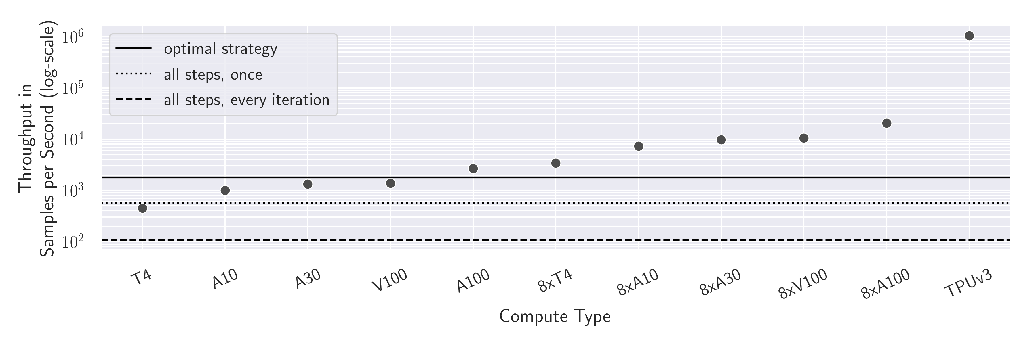
Figure 3. Throughput of ResNet-50 (He et al., 2016) for different hardware configurations. Black lines show the preprocessing throughput for the different strategies from Tab. 1. GPU profiling data from NVIDIA (NVIDIA, 2020) and TPUv3 by Ying et al. (Ying et al., 2018).

In this paper, we close this research gap by performing a comprehensive analysis of preprocessing pipelines from a broad range of different ML domains. In doing so, we present practical insights into the pipelines themselves as well as the methodologies to analyze bottlenecks and an automated tool to perform profiling of arbitrary pipelines. This opens up a new dimension in end-to-end ML system optimizations, which was not considered in prior works that targeted the pipeline optimization with respect to the model accuracy (Mohan et al., 2021; Kang et al., 2020).

Our contributions are:

1. We profile seven different real-world pipelines and define the trade-offs and characteristics that allow practitioners to improve existing pipelines by optimizing at the location with the greatest impact on the training throughput. This way, we could improve training throughput by up to 3-13$\times$ compared to fully preprocessing once.

2. We provide lessons learned, where we summarize the problems and unexpected findings we encountered that can limit pipeline throughput. For example, we found that storage consumption can affect the throughput negatively in different ways. These insights can be used to clear up common misconceptions, and practitioners can be more aware of the impact the preprocessing pipeline has on the training performance.

3. We present an open-source profiling library that automates the decision of which preprocessing strategy to pick based on a user-defined cost model.

Our paper is organized as follows. In Section 2, we introduce a general model and terminology of preprocessing pipelines. The experimental setup and the library design are explained in Section 3. We present our pipeline analysis and our findings in Section 4. Our derived insights are summarized in Section 5. Related work is reviewed in Section 6. Other approaches for pipeline optimizations are discussed in Section 7 and we conclude the paper in Section 8.

2. Preprocessing Pipelines

We begin by describing the set of problems one faces when preparing a dataset for the training process. This includes determining the hardware requirements, the decision of where to preprocess the data, and when to preprocess, both of which decisions affect the training throughput in multiple ways.

The preprocessing pipeline can be split into steps which are ran once ($S_{\textbf{1}}-S_{\textbf{m}}$), called “offline” henceforth, and steps which are performed every iteration ($S_{\textbf{m+1}}-S_{\textbf{n}}$), called “online”. The set of preprocessing steps depends on the dataset and the model input, but generally, any transformation is a step, like cropping an image or encoding a word. A preprocessing strategy is processing up to (and including) a step offline, and the remainder of the pipeline is executed online. Such a split is accomplished by inserting a save step which encodes and writes the data to disk (after $S_{\textbf{m}}$), and a load step that reads that data from disk (before $S_{\textbf{m+1}}$).

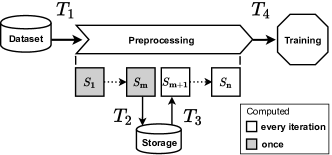
Figure 4. General DL preprocessing setup with different theoretical throughputs $T_{1}-T_{4}$ between the preprocessing steps $S_{\textbf{1}}-S_{\textbf{n}}$.

We conceptually divide the entire DL training process into three parts - the unprocessed dataset, the preprocessing pipeline, and the training (Fig. 4). They are all connected by four theoretical throughputs $(T_{1}-T_{4})$, which can become processing bottlenecks.

$T_{1}$:

is the read throughput from the dataset to the processing units which handle the offline preprocessing. This throughput is determined by hardware capabilities, such as storage devices, interconnects, processing capabilities, and software capabilities, such as file systems or DL frameworks.

$T_{2}$:

is the write throughput from the offline computed preprocessing step(s) ($S_{\textbf{1}}-S_{\textbf{m}}$) to a storage node. It is dependent on the throughput of each step, the interconnect to the storage node, and its write speed.

$T_{3}$:

is the read throughput from the storage node to the processing units which handle the online preprocessing ($S_{\textbf{m+1}}-S_{\textbf{n}}$) and is subject to the same restrictions as $T_{1}$.

$T_{4}$:

is the final preprocessing throughput when the data is ready to be fed into the training process. It is restricted by $T_{3}$, the online step(s) performance, and the interconnect to the training process. As $T_{4}$ limits the achievable training throughput, it is the most important to optimize.

In practice, it is often impossible to know the actual performance of future DL models or preprocessing pipelines. Only partial benchmarks are available to approximate the training throughput of popular DL models (NVIDIA, 2020). Even worse, there is no comprehensive throughput analysis of preprocessing pipelines, so one has to estimate the resulting $T_{4}$ throughput of a pipeline manually for every single deployment to prevent bottlenecks. Such an estimation is difficult to make, as there are many complexities involved.

One of those is the data encoding after step $S_{\textbf{m}}$, which serializes the entire dataset and places it on a storage device. The current default way to serialize datasets in two popular DL frameworks is the “pickle” encoding for PyTorch (Paszke et al., 2019), and Protobuf (Google, 2008) for TensorFlow (Abadi et al., 2016). Both encodings are not optimized for tensor data and may perform poorly. Applying an optimized compression algorithm may be useful but also introduces an additional online decompression step that may affect the $T_{4}$ throughput.

The deserialization throughput ($T_{1}$ and $T_{3}$) depends not only on the encoding but also on the storage solution and its interconnect to the nodes that run the preprocessing pipeline. A common storage solution in virtualized environments is Ceph (Weil et al., 2006), an object-based storage system. Such a complex and distributed system’s performance depends on the storage hardware and the computing power and must be evaluated on a case-by-case basis. Without benchmarks for specific hardware setups, it is unclear how to split the pipeline to achieve the maximum throughput (Ra, 2018; Mohan et al., 2021).

Another variable to consider is the offline preprocessing time, as this may delay the training start. Long preprocessing times can be prohibitive if not amortized by faster training.

Additionally, some preprocessing steps that feature data augmentation (e.g., random-cropping for images) or shuffling the dataset have to be done online because their results are not deterministic and can not be cached for future epochs.

Some preprocessing steps decrease the dataset size and can make it fit in memory, which would be beneficial over multiple epochs to remove network read effects. However, preprocessing steps can also be computationally expensive and would better be processed offline which can increase throughput, even if they increase the dataset size. Both scenarios can benefit the throughput, but it is not obvious to determine without profiling whether caching a dataset or removing a CPU bottleneck is more effective at increasing throughput.

In conclusion, deciding how to split a preprocessing pipeline into offline and online steps is a complex problem. The importance of the trade-offs may depend on individual scenarios, such as preexisting hardware or framework dependencies, which can not be chosen freely. To solve this problem and provide guidance and best practices to ML engineers and users, a comprehensive analysis of common DL pipelines is needed that provides a structured overview of the pipelines’ performance and insights about the individual steps’ trade-offs. It is also necessary to evaluate whether profiling a small sample of the entire dataset is sufficient to estimate the total processing time, storage consumption, and $T_{4}$ throughput. This could reduce profiling overhead. Finally, a software solution should automate the profiling to quickly generate insights for a specific setup to optimize any given pipeline.

3. Experiments

We analyze four different ML domains to showcase trade-offs in preprocessing pipeline optimizations: CV, NLP, Audio, and non-intrusive load monitoring (NILM). We evaluate the pipelines with in total seven different datasets in order to compare the impact of different encodings and image resolutions on the respective pipeline’s performance. Every pipeline is based on common preprocessing steps from popular models and datasets in their respective domains. We assume that the training throughput is unbounded for our analysis, as we are interested in maximizing $T_{4}$ irrespective of the actual model. This section showcases the design of our profiling library, the individual pipelines and defines the experimental setup.

3.1. PRESTO Library

After initial manual profiling attempts, we decided to create the Preprocessing Strategy Optimizer (PRESTO) library that automates the generic pipeline profiling process. The library can be used with any preprocessing pipeline written with the TensorFlow tf.data API (Murray et al., 2021), and hence, is readily applicable to different use cases.

PRESTO contains a Strategy wrapper class that splits the preprocessing pipeline at any given step into an offline and online part. This is done by inserting a serialization and loading step at the split position with the TFRecord format, a wrapper around the Protobuf encoding (Google, 2008) for TensorFlow. Additional parameters include the parallelism, sharding, caching behavior, and compression format, as well as the temporary logging directory.

The strategy wrapper class executes the entire preprocessing pipeline through the tf.data API. We simulate the training process by accessing the sample tensor’s shape member to measure the preprocessing throughput without training an actual model. This allows us to profile the preprocessing pipeline’s throughput by calling the profile_strategy() function. It accepts two parameters which have to be set manually: sample_count and runs_total. While it is useful to get an initial understanding of a pipeline’s performance with less samples, some bottlenecks only show after local caches are full or a network link is used to its maximum capacity, so that we recommend profiling with the entire dataset.

Profiling focuses on three key metrics - preprocessing time, storage consumption and throughput - which can be easily tracked by internal Python code. For more in-depth information, dstat is executed in parallel and provides specific system-level information, like disk read/write loads and network traffic in case of network storage. These stats and additional metadata, like a unique hash and the split position, are returned as Pandas dataframes (Wes McKinney, 2010).

After the profiling is finished, the StrategyAnalysis class summarizes the findings and provides a semi-automatic way to pick the best strategy based on an objective function. The function normalizes the individual metrics to the range of $[0,1]$ based on their minimum and maximum values and multiplies them by user-defined weights $w_{p,s,t}$. Let preprocessing time be p, storage consumption s, and throughput t as vectors of the respective values for all strategies:

$$f(w_{p},w_{s},w_{t},\textbf{p},\textbf{s},\textbf{t})=w_{p}\times|\textbf{p}|+w_{s}\times|\textbf{s}|+w_{t}\times|\textbf{t}|$$

The weights $w_{p,s,t}$ are can be defined manually, based on the user’s objective. As an example, we want to find the optimal strategy to apply hyperparameter tuning on a model before a deadline. That means we want a low preprocessing time and the highest possible throughput, while the storage consumption is irrelevant. In this case, the weights would look as follows:

$$(w_{p},w_{s},w_{t})=(1,\;0,\;1)$$

On the contrary, if we have access to a cluster with a lot of compute power and are not in a race against time, it will be preferable to sort only by throughput $(w_{p,s}=0,w_{t}=1)$, which is a good default configuration. This procedure can be applied to every strategy, which can have different parallelization, sharding and compression options and lead to new trade-offs. More complex objective functions can feature cloud providers’ processing and storage prices. We presume that renting a low-cost VM and profiling the different strategies could probe the infrastructure, i.e., network bandwidths. This allows us to extrapolate the processing performance by tensor-specific CPU benchmarks like PASTA (Li et al., 2020) for high-cost VMs. We provide our library as an open-source project at https://github.com/cirquit/presto.

3.2. Pipelines

We profiled seven pipelines from four different domains and designed them to represent popular DL models. Table 2 shows the seven datasets we used to profile the pipelines with their storage consumption, sample count, and format. The datasets and pipelines show a variety of common formats, and different intermediate sizes, e.g., the NLP pipeline has a strategy that increases the initial storage consumption by $64\times$, while NILM has a strategy that decreases the initial storage consumption by a factor of $12\times$ (Fig. 6). The pipelines were implemented with the tf.data API (Murray et al., 2021) which automates pipeline execution and allows us to parallelize computations easily. We define a sample in this context as data that is used as input for a DL model.

The naming of the steps in the pipelines follows a common pattern. First, the data is read from disk (unprocessed). After reading the dataset from disk, a concatenation step transforms the input files into a single TFRecord binary in order to allow for efficient sequential read access (concatenated). The concatenation step was technically not feasible for the Audio pipeline, and was omitted for the NILM pipeline as the raw data was already stored in concatenated binary form. Then, the data is decoded into a tensor format (decoded). Finally, additional transformation steps can be applied to bring the data into a format suitable for the training process. Generally, the steps have two characteristics: the online processing time and the relative increase or decrease of storage consumption. We explain the trade-off between these two characteristics in Sec. 4.1, which can change for the same step just by using different datasets, e.g., decoding can increase or decrease the storage consumption depending on the initial file encoding (e.g., JPG vs. PNG).

The performance of preprocessing steps depends not only on the implementation of the step itself, but also on its position in the pipeline and on the input data. We specifically showcase this behaviour in Sec. 4.6 by changing the position of a new step in an existing profiled pipeline.

Dataset	Pipeline	Sample Count	Size in GB	Avg. Sample Size in MB	Format
ILSVRC2012 (Russakovsky et al., 2015)	CV	1.3M	146.90	0.1147	JPG
Cube++ JPG (Ershov et al., 2020)	CV2-JPG	4890	2.54	0.5203	JPG
Cube++ PNG (Ershov et al., 2020)	CV2-PNG	4890	85.17	17.4176	PNG
OpenWebText (Aaron Gokaslan, 2019)	NLP	181K	7.71	0.0427	TXT
CREAM (Jorde et al., 2020)	NILM	268K	39.56	0.1477	HDF5
Commonvoice (en) (Ardila et al., 2019)	MP3	13K	0.25	0.0197	MP3
Librispeech (Panayotov et al., 2015)	FLAC	29K	6.61	0.2319	FLAC

Table 2. Metadata of all profiled datasets.

3.2.1. CV

We profile three datasets with the CV pipeline (Fig. 2) to analyze the performance under different image resolutions and encodings. ILSVRC2012 (Russakovsky et al., 2015) is a low resolution, JPG encoded subset of ImageNet (Deng et al., 2009) and is a popular and commonly acknowledged dataset for visual object recognition. Cube++ is a high-resolution dataset and comes in two flavors: as 16-bit encoded PNGs and JPGs (Ershov et al., 2020). The difference in storage consumption between the two encodings allows for a direct comparison of the decoding performance. The images from Cube++ are roughly $5\times$ larger than in ILSVRC2012, which allows to analyze how much the image resolution affects the throughput of each strategy. Details of this pipeline have been discussed in Section 1.

3.2.2. NLP

The NLP pipeline (Fig. 5(a)) is based on GPT-2 (Radford et al., 2019), a popular transformer-based model which tries to predict the next word based on the textual input. We used the dataset from the corresponding open-source implementation (Aaron Gokaslan, 2019) of OpenWebText, which was replicated from the GPT-2 paper. Our version of the dataset is an early iteration and takes up 8 GB compared to the most current one at 12 GB. The dataset consists of HTML content from scraped URLs that have been upvoted on Reddit, a social media platform, as an indicator of human interest and intelligible content. It is stored as multiple text files.

The preprocessing starts with reading text files (concatenated) and decoding the actual textual content (decoded) with the same HTML parsing library (newspaper (Ou-Yang, 2013)) as GPT-2. Each word is encoded into an int32 via Byte Pair Encoding (Sennrich et al., 2016) (bpe-encoded), which is then looked up in a word2vec embedding (Mikolov et al., 2013) that returns a float32 tensor of dimension $1\times 768$ (embedded). This vector is stacked for every word in the text, resulting in an $n\>\times\>768$ tensor, the final model input. These preprocessing steps’ complexity depends on the tokenization model and the final embedding, making their performance hard to predict.

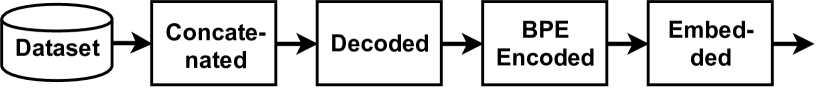
(a) NLP

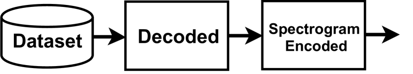
(b) MP3 + FLAC

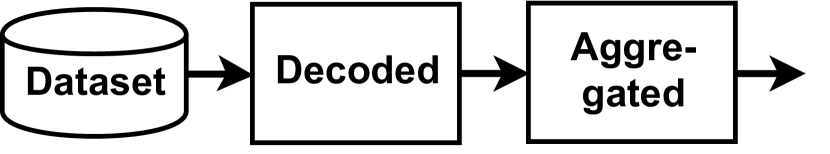
(c) NILM

Figure 5. Preprocessing pipelines

3.2.3. Audio Processing

For the audio pipelines, we took inspiration from Baidu’s Deep Speech model (Hannun et al., 2014; Amodei et al., 2016). Deep Speech is an RNN-based model that translates spoken audio samples to text. Both preprocessing pipelines (Fig. 5(b)) decode the compressed audio signal into the raw waveform (decoded) of the size $l\times r$, where $l$ is the sample duration in seconds and $r$ is the sampling rate encoded as int16. The waveform is transformed using a short-time Fourier transform (STFT) with a window size of 20 ms and a stride of 10 ms. The spectrogram is then transformed using an 80-bin mel-scale filter bank, leading to a size $\frac{l-20ms+10ms}{10ms}\times 80$ tensor encoded as float32 (spectrogram-encoded). The difference between the pipelines is their respective input format (MP3 vs. FLAC). In contrast to some implementations (Hannun et al., 2014), we do not convert the data to mel-frequency cepstral coefficients (MFCCs) because it has been found that DL models work as well or better without this transformation (Huzaifah, 2017; Purwins et al., 2019; Solovyev et al., 2020).

As datasets, we use the Mozilla Commonvoice 5.1 English corpus (Ardila et al., 2019) for MP3 files and the Librispeech dataset (Panayotov et al., 2015) for FLAC files.

3.2.4. NILM

Our signal processing pipeline is based on MEED (Jorde et al., 2019), a state-of-the-art event detection model used for non-intrusive load monitoring of electrical data. The task is to classify individual appliances based on the aggregated voltage and current reading measured on a building’s mains. These datasets typically have a very high frequency, e.g., 6,400-50,000 Hz (Anderson et al., 2012; Kriechbaumer and Jacobsen, 2018; Jorde et al., 2020) to provide information on subtle changes that can be useful for appliance identification.

We used CREAM (Jorde et al., 2020), a component-level electrical measurement dataset for two industrial-grade coffeemakers encoded as HDF5 files per hour. CREAM contains two datasets from two different coffee machines (X8 and X9), from which we used the larger X8 dataset because it takes up more than double the storage consumption of X9, i.e., totals 744 hours of 6.4 kHz sampled current and voltage. This dataset’s fundamental difference to the other datasets is the float64 encoding, which is favorable for NILM tasks (Kahl et al., 2017) but introduces additional storage consumption.

The pipeline starts by reading HDF5 files and extracts the voltage and current signals from them (decoded). They are sliced in 10-second windows, which results in a $2\times 64.000$ tensor of float64. Then, three aggregated values are computed: the reactive power (Barsim et al., 2014), the root-mean-square of the current, and its cumulative sum (Jorde et al., 2019; Trung et al., 2014; Zhu et al., 2018b) (aggregated). These aggregation operators work with a dataset period length of 128, which results in a tensor of size $3\times 500$ encoded as float64.

3.3. Experimental Setup

We execute our experiments on a virtual machine with 80 GB DDR4 RAM, 8 VCPUs on an Intel Xeon E5-2630 v3 8x@2.4 GHz with an Ubuntu 18.04 image on our OpenStack cluster. Our Ceph cluster, backed by HDDs, is used as a storage device via cephfs, with a $10$ Gb/s uplink and downlink. This storage is used for both storing the intermediate dataset representations as well as the unprocessed datasets. We repeat each experiment five times and we drop the page cache after every run to remove memory caching effects except for explicitly marked caching experiments. All experiments are run with 8 threads except for explicitly marked scalability experiments with a sharded dataset so that every thread has an assigned individual file to read in parallel. All experiments are executed with Python 3.7 and TensorFlow 2.4. Specific library versions are available in our GitHub repository.

4. Analysis

By profiling the preprocessing pipelines, we aim to provide insights about how to pick the optimal preprocessing strategy for a specific set of hardware, the datasets, and the characteristics of each pipeline. The goal is to maximize the $T_{4}$ throughput (Fig. 4) while keeping the storage consumption and offline preprocessing time low. Our analysis is focused on four core aspects:

Storage Consumption versus Throughput::

A high storage consumption can render extensive offline preprocessing useless or even counterproductive to achieve high throughput. This has two causes. First, the dataset may be split into many files, and the storage does not respond fast enough to random read access, leading to a storage bottleneck. Secondly, specific preprocessing steps (e.g., normalizing an integer range to floating points) inflate the data volume. This can lead to a lower throughput because the saved preprocessing time is outweighed by the increased data ingestion time (see Section 4.1).

Caching::

As a DL training process typically iterates over the dataset multiple times, there can be an increased throughput due to caching effects after the first epoch. However, this effect depends on whether the preprocessed training data fits into memory. Further, reading the cached dataset from memory can help to isolate processing bottlenecks from storage bottlenecks (see Section 4.2).

Compression::

Compression provides a way to trade off CPU overhead for en-/decode steps against smaller storage consumption. We profile each strategy with GZIP (Deutsch, 1996) and ZLIB (Deutsch and Gailly, 1996) compression and show under which circumstances compression improves the throughput (see Section 4.3).

Parallelization Capabilities::

Preprocessing steps can hinder performance if multi-core CPUs are not utilized effectively. Scalability bottlenecks may have a substantial impact on throughput. We compare the speedup of each preprocessing step under multi-threading and system-level caching in Section 4.4.

We also touch on shuffling (see Section 4.5) and discuss how to introduce new steps to an already profiled CV pipeline based on a case study in Section 4.6.

Threads	Files per Thread	Bandwidth	Latency	IOPS
1	1	219 MB/s	$4-10\mu\text{s}$	53400
8	1	910 MB/s	$4-10\mu\text{s}$	222000
1	5000	6.6 MB/s	$4-10\mu\text{s}$	1629
8	5000	40.4 MB/s	$4-10\mu\text{s}$	9853

Table 3. fio profile of our storage cluster

4.1. Storage Consumption versus Throughput

We profiled the throughput and storage consumption for all strategies of each pipeline in Figure 6. The theoretical network read speed to the HDD-backed Ceph storage cluster is capped at 1.25 GB/s (10 Gb/s) due to hardware limitations, but the actual rates differ based on the access pattern. To provide a pipeline-independent measurement, we profiled four workloads with the fio tool (et al., 2021b) to simulate both sequential and random file access with 5000 files of 0.2 MB each and with one 5 GB file, which is comparable to our unprocessed and concatenated strategies. Additionally, we tested the single-threaded performance compared to 8 threads with the same workload per thread. Table 3 shows that reading sequentially is 33$\times$ faster for single- and 22$\times$ faster for multi-threaded execution. While our single-threaded bandwidth is limited to 219 MB/s, the multi-threaded execution is close to the hardware cap with 910 MB/s. This helps to explain our main observations:

Pipeline	Throughput in SPS		Network Reads in MB/s
	unprocessed	concatenated	unprocessed	concatenated
CV	107	962	($\pm 3$) 12	($\pm 16$) 111
CV (SSD)	588	944	($\pm 8$) 68	($\pm 15$) 108
CV2-JPG	88	288	($\pm 11$) 46	($\pm 72$) 110
CV2-PNG	15	21	($\pm 37$) 270	($\pm 54$) 390
NLP	6	6	($\pm 0.2$) 0.21	($\pm 1.5$) 0.26
NLP (SSD)	3	3	($\pm 0.2$) 0.17	($\pm 1.2$) 0.16

Table 4. Throughput and average network read speeds for strategies with concatenation.

(1) Concatenating can increase throughput significantly.

An I/O bottleneck may arise when the storage cannot saturate the hardware bandwidth based on the data access pattern. Out of the four pipelines which have a concatenated strategy (CV, CV2-JPG, CV2-PNG, and NLP), we see that all CV-based pipelines have a throughput increase between 1.4$\times$ and 9$\times$ compared to the unprocessed strategy (Table 4). The individual differences in the throughput can be explained by the dataset size and the average storage consumption of a sample (Table 2). Due to the CV samples being smaller than the CV2-JPG samples, CV achieves 962 SPS compared to 288 SPS while having a similar network read speed of approximately 110 MB/s. The CV2-PNG dataset has a sample storage consumption of 17.4 MB and the network read speed increases from 270 MB/s to 390 MB/s with concatenation.

Contrary to CV-based pipelines, the NLP pipeline does not benefit from concatenating as the throughput stays at 6 SPS, indicating a CPU bottleneck. This bottleneck is resolved in the decoded strategy, where throughput increases significantly (Fig. 6(d)).

As an HDD-based storage solution is particularly vulnerable to random access bottlenecks, we additionally profiled the performance of the CV and NLP pipeline on an SSD-backed Ceph cluster. The CV unprocessed strategy had a throughput of 588 SPS, which is almost $6\times$ faster than the HDD experiments. However, at the concatenated strategy, both HDD and SSD reach roughly the same throughput (962 SPS vs. 944 SPS), i.e., at sequential access the SSD-backed storage is not faster. For NLP, the SSD storage did not provide a better throughput as it still faces the CPU bottleneck at the concatenated strategy.

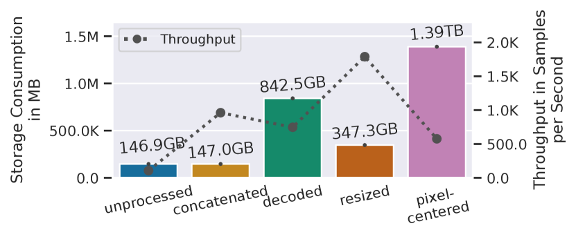
(a) CV

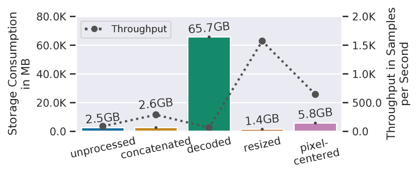
(b) CV2-JPG

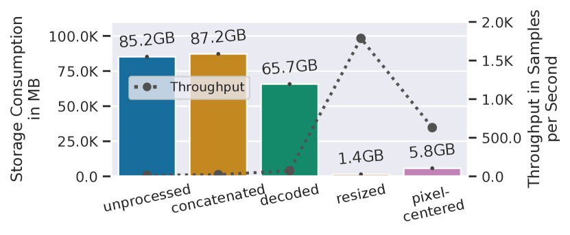
(c) CV2-PNG

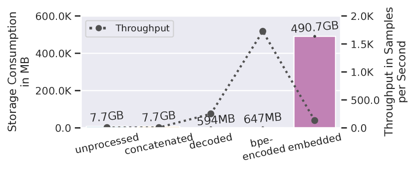
(d) NLP

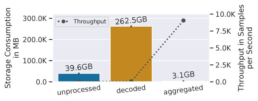
(e) NILM

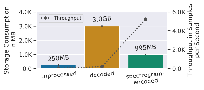
(f) MP3

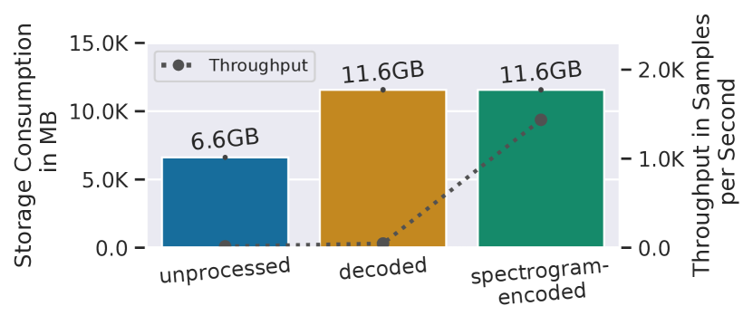
(g) FLAC

Figure 6. Storage consumption (left y-axis) for each dataset representation compared to the $T_{4}$ throughput (dotted line, right y-axis).

(2) The maximum throughput of a strategy is influenced by its storage consumption.

When the CPU performance in combination with a storage setup can saturate the hardware bandwidth (i.e., in our case, read data with 1.25 GB/s), then a maximum theoretical throughput can be calculated by dividing the bandwidth by the storage consumption per sample. This theoretical throughput is based on two steps. First, one reads a sample from the storage into memory. Second, one applies the online transformation steps in succession until the sample can be fed into the training process. The total time of these two steps defines the pipeline’s throughput (i.e., samples per second), hence also the network read speed (i.e., MB per second). In our case, the actual throughput we can achieve is bound by the multi-threaded read performance to our cluster, which is at 910MB/s with eight threads (Table 3). This profiled network read speed provides a baseline of the maximum possible throughput. The goal of every strategy should be to have a short enough transformation step to achieve this baseline read speed. In turn, if transformation steps are too long, such that the maximum read cannot be reached, we can assume a CPU bottleneck.

A characteristic result of how storage consumption affects the throughput of strategies can be seen in the CV, CV2-JPG, CV2-PNG and NLP pipelines (Fig. 6(a), 6(b), 6(c), 6(d)), where the last strategy has the least amount of online processing to do, but performs worse than its corresponding preceding strategy. An excellent example of this is the CV pipeline. At the last strategy, pixel-centered, we have an average network read speed of 585 MB/s and need to read 1.4 TB of data. This stands in contrast to the previous strategy, resized, which has a lower network read speed of 470 MB/s, but only needs to read 347 GB. Therefore, the resized strategy has a more than $3\times$ greater throughput of 1789 SPS compared to pixel-centered (576 SPS), even though resized applies more processing steps online. The cause of the increased storage consumption is that pixel-centered converts each pixel from an uint8 to a float32 which effectively quadruples the storage consumption. All our CV-based pipelines share this characteristic at different magnitudes, which results in the resized strategy having the best throughput.

The NLP pipeline has a similar issue with the embedded step, which slows down the throughput from 1726 SPS with bpe-encoded to 131 SPS with embedded (a factor of $13\times$). Applying the embedding step online is very computationally intensive, which yields a data ingestion of only 6 MB/s for bpe-encoded. One could think that preprocessing this step offline should improve performance. But this is not the case, because the storage consumption increases from 647 MB to 491 GB, such that the benefit of processing the embedding step offline is outweighed by the increased time to read the dataset.

The remaining pipelines, NILM, MP3 and FLAC (Fig. 6(e), 6(f), 6(g)), share the common characteristic that the last preprocessing step is the most computationally expensive one, which leads to the best throughput when processed offline. While they all have different storage consumption, none of the pipelines approaches the maximum possible network read speeds at their respective last strategy.

On first sight, this is counter intuitive. In the last strategy, there is almost no processing to be done except for decoding the read data. Why do these strategies not approach the network read limit? A deeper investigation leads to our following observation.

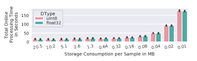
Figure 7. Profiling a synthetic 15 GB dataset with different datatypes and sample sizes.

(3) A high storage consumption per sample allows for easier I/O bandwidth saturation.

A deserialization step is applied onto every sample which is read from the storage to transform it from a bytestream into a tensor. We observed that an increasing sample size positively influences the I/O bandwidth of reading and deserializing. To provide a basis to our observation, we conduct an experiment with synthetic data that shows the effect of different sample sizes on the online processing time of reading and deserializing. We evaluate sample sizes from 0.01 MB to 20.5 MB with doubling increments while keeping a total storage consumption of 15 GB for both uint8 and float32 datatypes which are common in our real-world pipelines. To keep the same total storage consumption with different sample sizes we adapted the sample count, which ranged from 732 (20.5 MB) to 1.5M (0.01 MB) samples. Figure 7 shows the result that reading the same amount of data with different sample sizes has a major effect on the processing time. A dataset consisting of large (20.5 MB) samples takes less than half the processing time of small ($\leq 0.08$ MB) samples. At a sample size of 0.01 MB, it takes more than $11\times$ longer to process the 15 GB of data compared to 20.5 MB samples. Finally, the different data types do not have an impact on the processing time, as both uint8 and float32 show similar results.

A good example for this observation is the comparison of the decoded strategy between CV (Fig. 6(a)) and CV2-JPG (Fig. 6(b)). The average sample size is 13 MB for the decoded strategy of CV2-JPG with a network read speed of 828 MB/s, which indicates an I/O bottleneck. However, with the same strategy, the CV pipeline has a sample size of 0.6 MB and the average network read rate is at 491 MB/s, which is not even close to our maximum bandwidth. Notably, the CV pipeline has a lower computational load compared to CV2-JPG and has to read fewer data from storage with each sample due to the small sample size. But it still does not manage to saturate the I/O bandwidth. Therefore, the CV decoded strategy suffers from a CPU bottleneck. To further validate our assumption, we profiled the CV pipeline with 16 threads which increased the network read speed by 64 MB/s and improved the throughput by 142 SPS. The additional multi-threading also increased the throughput by 583 SPS and 100 SPS for the resized and pixel-centered, respectively. All last strategies like aggregated (Fig. 6(e)), spectrogram-encoded (Fig. 6(f), 6(g)), and embedded (Fig. 6(d)) share that characteristic and do not saturate the I/O bandwidth (96 MB/s, 317 MB/s, 564 MB/s and 315 MB/s respectively).

4.2. Caching

DL training jobs typically run over multiple epochs, which means the dataset is read multiple times and could benefit from being cached in memory after the first epoch. We evaluated the throughput of all pipelines over two epochs for all strategies. In this set of experiments, we do not flush the page cache after the first epoch. Our observations are as follows:

(1) Caching is not beneficial when the storage consumption is higher than the available memory.

If the data set is too large for the memory, the dataset is read completely from the storage at every epoch. Hence, throughput is not increased by caching. All strategies that have a storage consumption higher than 80 GB (Fig. 6) have the same throughput over all epochs (Fig. 8).

(2) Caching does not remove CPU bottlenecks.

Assuming that the dataset fits into memory, caching can only improve throughput significantly if there is no CPU bottleneck. Reading data from memory is much faster than from remote network storage, but the impact of fast data access can become insignificant when followed by computationally expensive preprocessing steps. An excellent example of this is the NLP pipeline (Fig. 8(d)). The first two strategies unprocessed and concatenated have the same throughput of 6 SPS over all epochs because decoding is very compute intensive while the datasize is relatively small (7.7 GB). Then, after decoding the data (594 MB), we face a new computationally expensive step, byte-pair encoding, which transforms the text into integers and increases the storage consumption to 647 MB. This is followed by the embedding step, which also takes much time. All of these strategies face a CPU bottleneck while having a storage consumption that allows the data to be cached. Finally, at the embedded strategy, the dataset only needs to be read from the storage, but grows in size to 490.7 GB, such that caching has no impact on throughput.

Similar CPU bottlenecks can also be observed in the unprocessed strategies of CV2-PNG, NILM, MP3 and FLAC (Fig. 8(c), 8(e), 8(f), 8(g)), the concatenated strategies of CV2-{JPG,PNG} (Fig. 8(b), 8(c)) and the decoded strategies of MP3 and FLAC. The remaining strategies (resized, pixel-centered, aggregated, spectrogram-encoded) benefit from caching the most as they have low storage consumption and are not followed by computationally expensive steps. However, caching improves the throughput with differing factors ($1.1\times$-$4.2\times$), which results in the next observation.

(a) CV

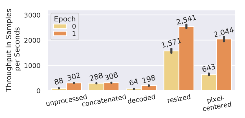
(b) CV2-JPG

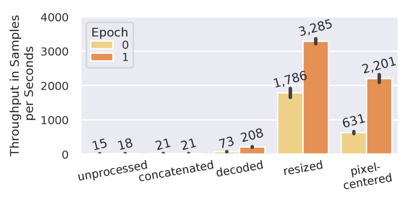
(c) CV2-PNG

(d) NLP

(e) NILM

(f) MP3

(g) FLAC

Figure 8. Effects of caching on $T_{4}$ throughput for all pipelines.

(3) System-level caching performance is affected by the storage consumption per sample.

While cached data removes the performance impact of remote storage, the preprocessed dataset still has to be fetched from memory and deserialized. We confirmed this by comparing the trace log between epochs. To examine the memory bandwidth, we used sysbench (et al., 2021a) to profile our memory which resulted in 166 GB/s. This should theoretically yield a multiplicative increase in throughput, which we do not achieve because we are not close to the maximum I/O bandwidth (cf. Sec. 4.1 observation (3)).

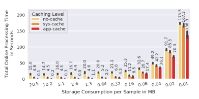
Figure 9. Online processing time for different caching levels and sample sizes of a synthetic 15 GB dataset.

We investigate this observation by profiling synthetic float32 datasets with different sample sizes with both system- and application-level caching (Fig. 9). At the lower end of storage consumption, starting with 0.16 MB per sample, reading smaller samples takes increasingly longer. The smaller the sample size, the more processing time the deserialization takes, which lessens the final throughput of the cached dataset. At 0.04 MB and lower, the processing time when data is cached in memory (sys-cache) is comparable to the case where data is on storage (no-cache), nullifying the effects of caching.

Our real-world experiments show the same behaviour. The storage consumption per sample for MP3 is 0.08 MB at the spectrogram
-encoded strategy, while having a relative throughput increase of $1.6\times$ (Fig. 8(f)) with caching. Meanwhile, the FLAC pipeline has a storage consumption of 0.4 MB per sample with the same strategy and increases its throughput by $4.2\times$ (Fig. 8(g)) with caching. The NILM pipeline shows almost no increase in throughput ($1.1\times$) over multiple epochs (Fig. 8(e)) as the sample size is only 0.012 MB.

While this is interesting, system-level caching via the page cache is somewhat unsatisfactory, since one wants to cache the tensor data and not be bottlenecked by the deserialization. The TensorFlow function tf.data.Dataset.cache caches the deserialized tensors in memory, avoiding deserialization overheads. This leads us to our fourth observation.

Pipeline	System-level	Application-level	Sample Size
CV2-JPG	$3.3\times$	$15.2\times$	1.18 MB
CV2-PNG	$3.5\times$	$14.5\times$	1.18 MB
FLAC	$4.2\times$	$8.0\times$	0.41 MB
MP3	$1.6\times$	$2.2\times$	0.08 MB
NILM	$1.1\times$	$1.4\times$	0.01 MB

Table 5. Throughput increase for different caching level compared to no caching of of each pipeline’s last strategy.

(4) Application-level caching is more efficient than system-level caching, but is still affected by the storage consumption per sample.

To understand how application-level caching affects the performance, we profiled all pipeline’s respective last strategies, as well as our synthetic 15 GB datasets again with application-level caching. The results of the synthetic datasets in Fig. 9 (app-cache) show that application-level caching is faster, but there is the same pattern of increasing processing time with a smaller sample size. The online processing time with application-level caching consists solely of reading the samples from memory. We can calculate the time spent on deserialization by subtracting the app-cache time from sys-cache time. By dividing with the sys-cache time, we can get the percentage of the time spent on deserialization. For the sample sizes 20.5 MB to 5.1 MB we spend 94-98% time on deserialization ($\frac{4.8-0.1}{4.8}$), compared to 14-18% for 0.08 MB to 0.01 MB ($\frac{167.3-138.3}{167.3}$). Hence, the largest relative gains with application-level caching can be achieved with large sample sizes.

Our real-world pipelines have shown a similar throughput improvement compared to system-level caching when the dataset fits into memory (Tab. 5). The decline in throughput improvement with both caching levels is directly correlated with a smaller sample size. The last strategies of the CV and NLP pipelines failed to run with application-level caching as the dataset did not fit into the cache (cf. Sec. 4.2 (1)).

4.3. Compression

Storage consumption has shown to be an important factor for throughput. Compression adds a new possibility to decrease storage consumption at the cost of an offline compression step and an online decompression step. For compression to provide a benefit, the gains of decreased data size must outweigh the computational overheads. A common metric to evaluate compression on storage consumption is the space saving percentage. For example, if the size did not change after compression, the space saving is 0%. When it changes from originally 5 GB to 1 GB, the space saving is 80%. We omitted the unprocessed strategy for all pipelines because accessing single files is bound by the random access performance of the storage (cf. Sec. 4.1 (1)) and compression does not help with this issue.

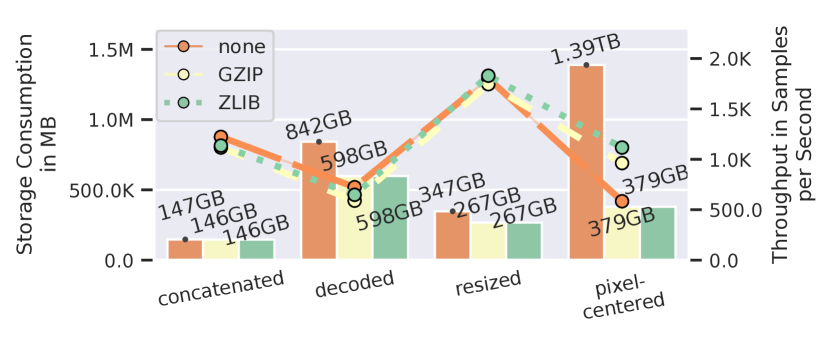
(a) CV

(b) CV

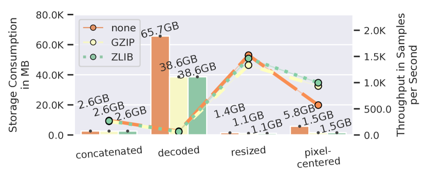
(c) CV2-JPG

(d) CV2-JPG

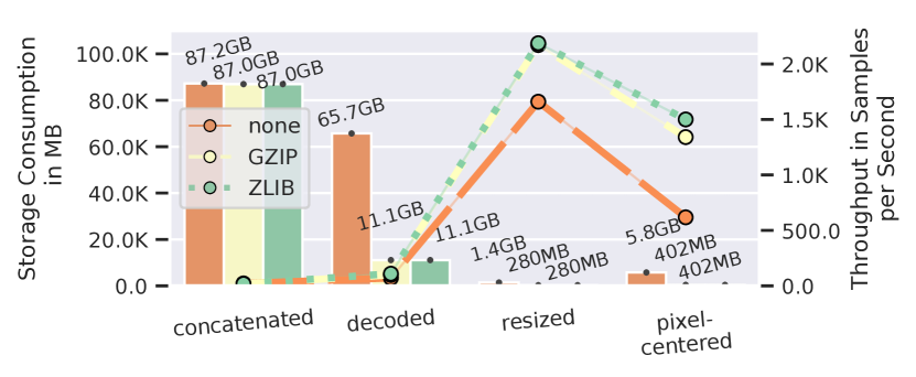
(e) CV2-PNG

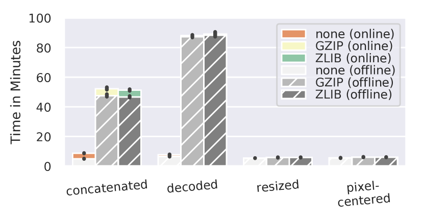
(f) CV2-PNG

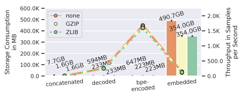
(g) NLP

(h) NLP

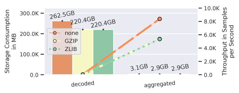
(i) NILM

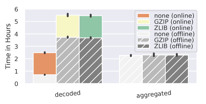
(j) NILM

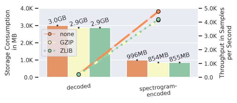
(k) MP3

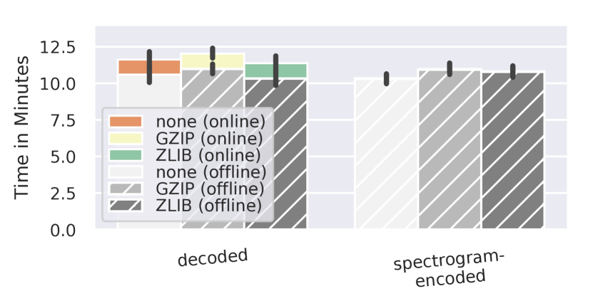
(l) MP3

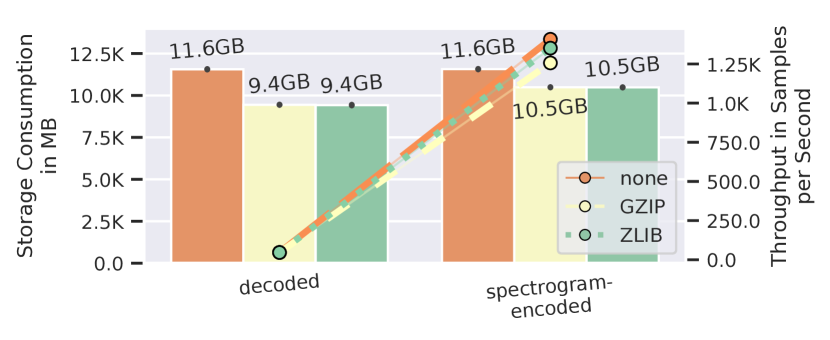
(m) FLAC

(n) FLAC

Figure 10. Left column: Storage consumption compared to $T_{4}$ throughput (dotted lines) with compression. Right column: Offline (grey hatched bars) and online processing time (colored) with compression.

The results of our compression experiments are shown in Fig. 10. We make the following observations:

(1) High space savings do not guarantee improved throughput.

Space saving affects the throughput positively for some, but not all strategies. All CV-based pipelines had an increase in throughput with compression between $1.6\times$ and $2.4\times$ at pixel-centered where space saving is between 73% and 93% (Fig. 1, 10(c), 10(e)). In this case, the faster read time in total was beneficial compared to the cost of the additional decompression step.

In contrast, the strategies of the NLP pipeline have a space saving between 28% and 80%, but none of them had a throughput increase (Fig. 10(g)). The reason for that is that every strategy was bound by a computationally expensive CPU step except the last strategy embedded. At embedded, the dataset is only read from disk and deserialized, but the space saving of 28% was not enough to benefit the total throughput.

The same effect becomes visible when comparing the strategies decoded and resized between the CV2-PNG and CV2-JPG pipelines (Fig. 10(c), 10(e)). The only difference between the pipelines is the encoding of the images, with JPG being a lossy storage format, while PNG is lossless. The CV2-PNG pipeline has a better space saving with compression with the decoded strategy (83%) compared to CV2-JPG (41%). This results in a throughput increase by $1.5\times$ for CV2-PNG compared to the 89% throughput deterioration at CV2-JPG. The resized strategy with the PNG images has a space saving of 81% and improves the throughput by $1.3\times$, while JPG only saves 24% of space and reduces the throughput to 96%. The compression artifacts introduced by the lossy JPG encoding affect the space saving of both GZIP and ZLIB negatively.

All the other pipelines, NILM, MP3 and FLAC, slow down with compression and have a varying space saving between 0.3-41.2% (Fig. 10(i), 10(k), 10(m)). When comparing the different compression types, ZLIB was slightly faster and had a comparable space saving to GZIP, except for NLP’s bpe-encoded, where it was slightly slower compared to GZIP.

(2) Offline compression and write time can be volatile.

When compressing a dataset, the processing time is increased by the compression algorithm, and decreased by the lower write time due to lower storage consumption. The balance between these steps is not predictable from our observations, as the CV2-PNG pipeline shows (Fig. 10(f)). With the concatenated strategy and a space saving of only 0.3%, it takes $9.6\times$ longer to save the dataset to storage. The strategy decoded has a space saving of 83% and takes $13.5\times$ longer for offline processing. The next strategies, resized and pixel-centered, have a space saving of 80%-93% and only take 1.08-1.1$\times$ longer. Compared to a slightly worse space saving of 74% with the pixel-centered strategy at the CV2-JPG pipeline (Fig. 10(d)), the offline processing time is increased by $6.1\times$.

Generally, we see examples of a high space saving and no effective increase in offline processing time in NLP (Fig. 10(h)), a low space saving with a higher offline processing time in NILM (Fig. 10(j)) and CV2-PNG concatenated (Fig. 10(f)), and low space saving with no effective increase in offline processing time in MP3 (Fig. 10(l)), FLAC (Fig. 10(n)), and CV concatenated and resized (Fig. 1). Space saving does not seem to be a good predictor at how the compression will affect the offline processing time.

4.4. Parallelization Capabilities

Figure 11. Reading a synthetic 15 GB dataset with different sample sizes to compare multi-threaded scalability.

(a) CV no-cache

(b) CV sys-cache

(c) CV2-JPG no-cache

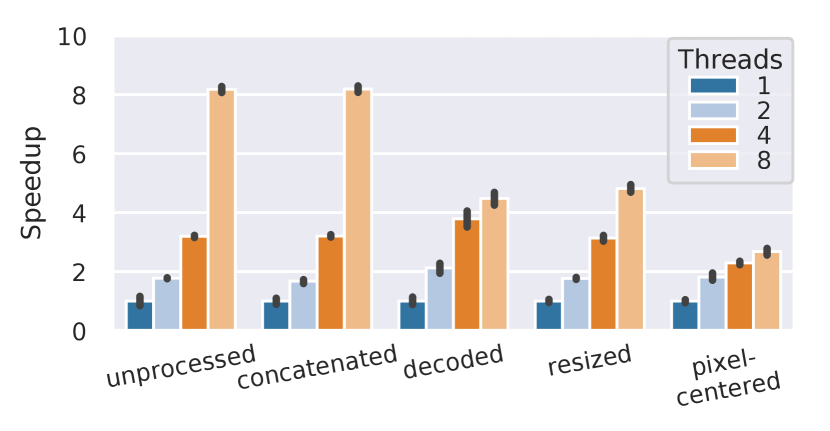
(d) CV2-JPG sys-cache

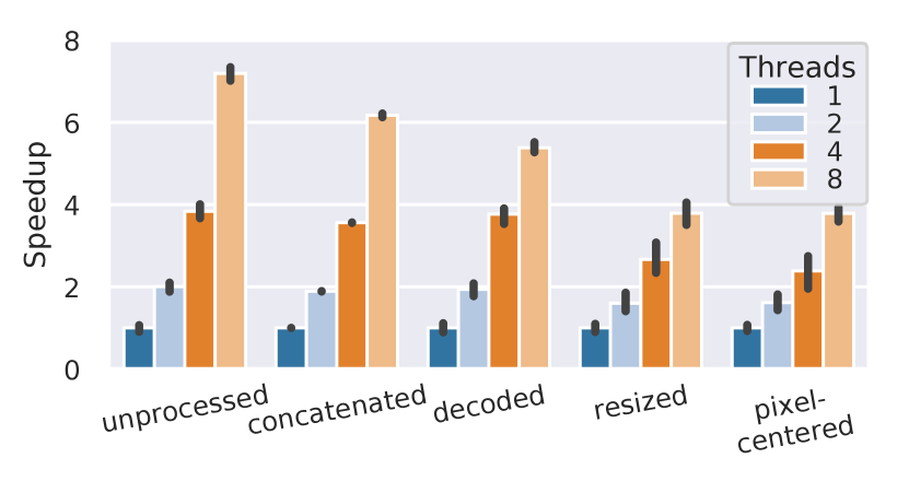
(e) CV2-PNG no-cache

(f) CV2-PNG sys-cache

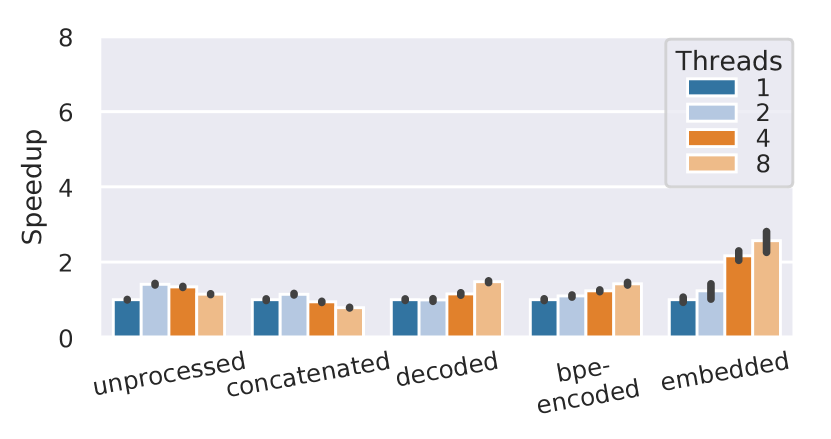
(g) NLP no-cache

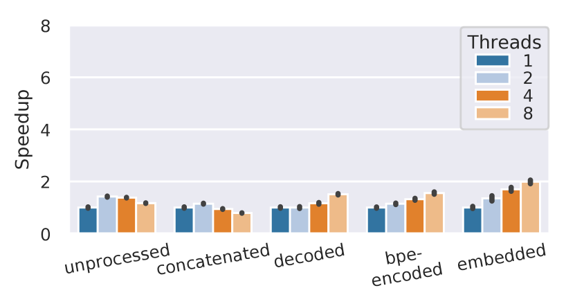
(h) NLP sys-cache

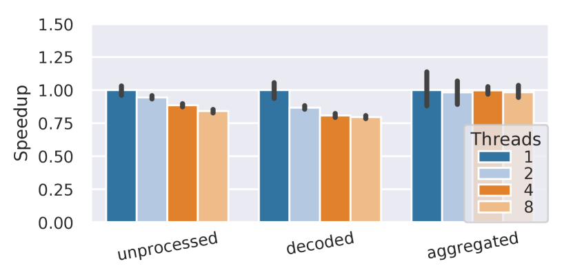
(i) NILM no-cache

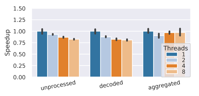
(j) NILM sys-cache

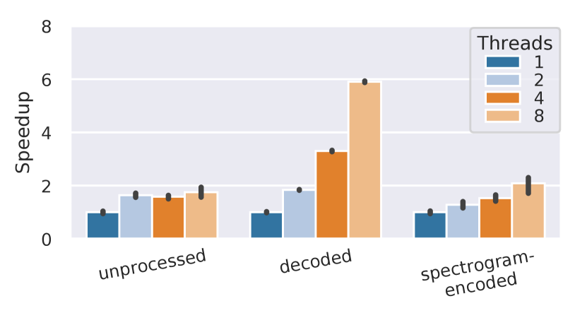
(k) MP3 no-cache

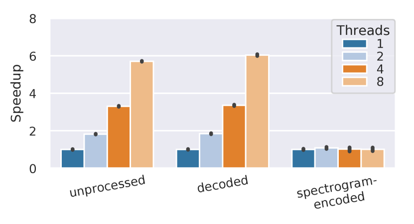
(l) MP3 sys-cache

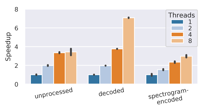
(m) FLAC no-cache

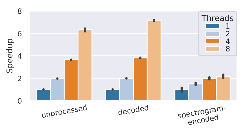
(n) FLAC sys-cache

Figure 12. Speedup at 8000 samples. Left column: No caching. Right column: System-level caching.

We analyzed the parallelization capabilities of each pipeline under multi-threading, as this is one of the best practice recommendations to speed up data pipelines and remove I/O bottlenecks (Google, 2020). We compared the speedup of each strategy by running it with 1, 2, 4, and 8 threads over two epochs with system-level caching enabled (Fig. 12). The profiling was done with a fraction of the dataset (up to 8000 samples) so that the second epoch could be fully cached for each pipeline to compare the speedup with system-level caching. We make the following observations:

(1) A small storage consumption per sample hinders multi-threaded performance. We know from the previous Sections 4.1 and 4.2 that a small storage consumption per sample affects the online preprocessing time negatively. However, how does it affect multi-threaded execution? To analyze this, we reused the same synthetic 15 GB float32 dataset with different sample sizes to compare their multi-threaded read and deserialization time. The results in Fig. 11 show a similar trend as before, with a speedup of close to 1$\times$ for the 0.01 MB sample sizes. This means that processing small samples with a single thread takes equally long as with eight threads. We traced the issue down to an increased amount of context switches with smaller sample sizes (100,000 per second at 0.01 MB compared to 5,000 per second for 20.5 MB). Additionaly, as we extracted from the trace log, every thread only processes a single sample at a time and is finished faster with smaller sample sizes before being scheduled again. Scheduling a thread to process a new sample induces so much overhead that multi-threading can not be effective at small sample sizes.

A good example from our real-world pipelines is NILM (Fig. 12(i)) at the aggregated strategy, which has no effective speedup due to a sample size of 0.01 MB. Even when reading the dataset from memory (Fig. 12(j)), there is virtually no change in speedup. Every last strategy from each pipeline has as slightly worse speedup when reading from memory (sys-cache) than when reading from storage (no-cache) (Fig. 12). The reason for this is that memory provides a higher bandwidth, so reading data is fast, even with a single thread. Therefore, the effect of context switches is highlighted even more compared to the case where the slower network read speeds affects the total processing time additionally.

(2) Inefficient preprocessing can reduce multi-threading scalability.

While most of the scaling issues like bpe-encoding in NLP can be explained with a small sample size (0.003 MB), we also observed slowdowns (speedup $<1.0$), which have a different root cause. This happens with the first two strategies of NILM (Fig. 12(i), 0.15 MB and 0.98 MB) and NLP (Fig. 12(g), 0.04MB), which are not alleviated by reading from memory (Fig. 12(j),  12(h), respectively). This points to a processing issue. One thing that both unprocessed, concatenated (NLP) and decoded (NILM) have in common, is that they are using external Python libraries like NumPy and newspaper wrapped in a tf.py_function, while all the other preprocessing steps are provided by the TensorFlow library.

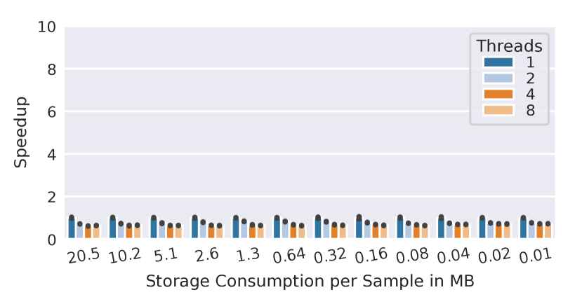
(a) NumPy RMS

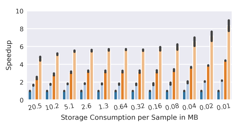
(b) TensorFlow RMS

Figure 13. Speedup of applying RMS to a synthetic 15 GB dataset with different sample sizes implemented in NumPy and TensorFlow.

To test how external libraries affect the throughput, we created a new preprocessing step which applies the root-mean-square (RMS) function with a period of 500 over the entire sample, leaning on a similar computation from the NILM pipeline. We implemented this step both with NumPy and TensorFlow, and we profile our synthetic datasets with steps applied online individually. The results in Fig.13 show that the NumPy implementation has the same slowdown as NILM and NLP for all sample sizes, whereas the TensorFlow implementation shows a speedup between 4-8$\times$ for eight threads. However, while the NumPy implementation does not scale, it is still 2.9$\times$ faster with a single-threaded processing time of 650 seconds compared to TensorFlow’s 1905 seconds with eight threads at the 20.5 MB sample size. In other words, it pays off to use the less scalable but more efficient implementation in NumPy instead of the native implementation in TensorFlow.

(3) Random file access performance can affect the speedup. We have already discussed the impact of concatenation in Sec. 4.1 (1) and how random file access can hinder achieving high throughput and bandwidth utilization. By running the multi-threading experiments with system-level caching enabled, we can isolate the effect of random file access on speedup. For example, the unprocessed strategy of the MP3 pipeline (Fig. 12(k)) has a speedup of $2\times$ when reading from storage with eight threads, versus a speedup of $6\times$ when reading from memory (Fig. 12(l)). This shows that decoding does in fact scale well. The same effect changes the speedup of the FLAC pipeline from 4$\times$ (Fig. 12(m)) to 6$\times$ with eight threads (Fig. 12(n)).

4.5. Shuffling

A common technique in DL is to change the order of the dataset in every epoch, so the optimizers do not see the same gradients in mini-batches. There are a few different approaches to shuffling the dataset, which include sampling from the dataset with- or without replacement (De Sa, 2020; Haochen and Sra, 2019; Yun et al., 2021). Irrespective of which algorithm is used to modify the order of the dataset, it is a very memory-intensive problem, as the entire dataset has to be loaded into RAM. One solution is to create a buffer that fits into the memory and use a with-replacement sampling strategy to iterate over the entire dataset in a pseudo-random fashion (Google, 2021), similar to reservoir sampling (Vitter, 1985).

We implemented and profiled this approach with multiple sample counts, which confirms the naive assumption that the per-sample processing time for shuffling is constant. That means that shuffling has a linear relation to storage consumption and is not specific to a pipeline or dataset. The difference in per-sample processing time between shuffling and not shuffling for each sample size is $(\pm 0.5)$ 9.6ms on average. An additional characteristic is that the initial call to allocate a buffer is amortized with a bigger sample size, which manifests itself in the increasingly faster per-sample time with incremented sample sizes.

PRESTO’s profiling can help to find the optimal place in the pipeline where shuffling should be applied. As the storage consumption of a strategy does not affect the runtime of shuffling, we do not recommend making shuffling part of the strategy selection. However, once a strategy is determined, we suggest to shuffle after the online pipeline step that yields the smallest data size. If we consider a fixed-size buffer for shuffling, the highest number of samples can be fit into the buffer when the size of the data sample is smallest. The higher the number of samples in the buffer, the higher the entropy; this, in turn, leads to a better approximation of the “true” gradient (Mustapha et al., 2020; Kingma and Ba, 2015).

4.6. Modifying the Pipeline

We added an additional preprocessing step to the CV pipeline to showcase how the trade-offs can shift in an already profiled pipeline. We decided on adding a step that converts images from RBG to greyscale because this is a common preprocessing step that affects the storage consumption and is not obviously compute intensive. To evaluate how an additional step will affect the pipeline performance, we profiled two setups: before and after the pixel-centered strategy.

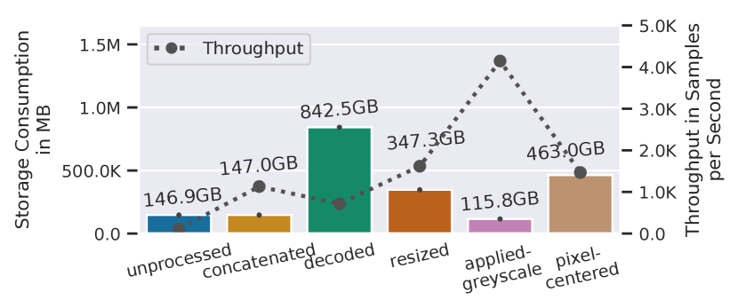
(a) Before Pixel Centering

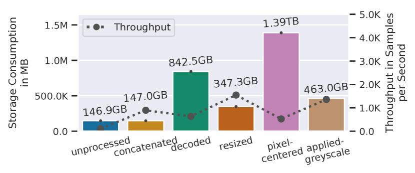
(b) After Pixel Centering

Figure 14. Storage consumption (left y-axis) and throughput (right y-axis, dotted line) comparison of adding a greyscale transformation before and after the pixel centering.

Before discussing the results, we explain the characteristics of the new applied-greyscale strategy and compare it to resized. Converting a 3-channel image to greyscale should decrease the storage consumption by 3$\times$, because we only need a single channel with the same datatype. The resized strategy reduces the size by 2.4$\times$ for the CV dataset, which is dependent on the average image resolution. Adding greyscaling will also affect the throughput of pixel-centered as the final storage consumption will be reduced as well.

The results in Fig. 14 show the effect of the additional greyscale step on the storage consumption and throughput. First of all, applying the greyscale step before the pixel-centered strategy increases the maximum throughput of the pipeline by 2.8$\times$, from 1513 SPS with resized (Fig. 14(b)) to 4284 SPS with applied-greyscale (Fig. 14(a)). While the last strategy of both setups performs similary, applying preprocessing steps that reduce the storage consumption consecutively increases the throughput for intermediate strategies. We additionally evaluated a setup where the resize and greyscale steps are interchanged before the pixel centering, but there was no significant difference in performance to Fig. 14(a). The second setup with the last strategy applied-greyscale increases the throughput from 534 SPS at pixel-centered to 1384 SPS by reducing the data size from 1.4 TB to 463 GB. This supports our observation (2) from Sec. 4.1 that steps which reduce storage consumption should be investigated with priority when searching for the best performing.

5. Lessons Learned

We find it important to summarize our findings more generically for both DevOps and ML practitioners so that they can use the PRESTO library and the generated insights for future analysis. These lessons are based on the analysis in Section 4.

(1) Storage consumption is an important characteristic when estimating throughput. We gravely underestimated the effect of storage consumption before conducting this study. The impact of storage consumption is a multi-faceted one, as it affects the storage hardware, its interconnects, the deserialization process and multi-threading capabilities. A small total storage consumption performs best if not throttled by a CPU bottleneck, and steps that reduce data size should be prioritized when searching for the best performing strategy. However, small sample sizes ($\leq 0.08$ MB) increase the online processing time dramatically irregardless of reading from storage or from memory and can be a reason for an underutilized I/O bandwidth. These two observations combined are the reason why fully preprocessed datasets did not yield the best throughput in 4 (CV, CV2-PNG, CV2-JPG, NLP) out of 7 pipelines.

(2) Multi-threading usually improves throughput, but the speedup can be limited for various reasons. Parallel execution of a pipeline is not a silver bullet when trying to speed up preprocessing. First of all, various issues can impede parallel speedup, such as calling external Python libraries or dealing with extremely short-running preprocessing tasks at small sample sizes. But even when parallel speedup of a strategy is reasonably good, a different strategy with a lower data volume to be read from storage may perform much better.

(3) It is recommended to use application-level caching whenever possible. Whenever the dataset fits into memory, application-level caching increased the throughput in our experiments by up to 15$\times$ with a high sample size. Application-level caching improved the throughput compared to system-level caching by a factor of 1.3-4.6$\times$, and should be preferred as the deserialization of cached files can slow down the pipeline.

(4) Compression can be useful when not facing a CPU bottleneck. Compression can increase the throughput by a factor of 1.6-2.4$\times$ under few conditions: a high enough space saving of 73-93% and the absence of computationally expensive processing steps. However, estimating the space saving, as well as the decompression time is hard. Additionally, applying compression can increase the offline processing time between 1.1$\times$ and 13.5$\times$ compared to no compression. The overheads of compression should be taken into account and carefully weighted against I/O savings.

6. Related Work

I/O profiling was already done in a micro-benchmark for TensorFlow by Chien et al. (Chien et al., 2018) which focused on different file systems and the check-marking functionality. In their experimental setup with AlexNet (Krizhevsky et al., 2012c), the training data prefetching eliminated the effective preprocessing time, similar to our CV pipeline with the unprocessed strategy.

OneAccess, a unified data loading layer, functions as middleware for preprocessing and helps to run ML jobs on multiple nodes more efficiently by removing duplicate processing for hyperparameter tuning (Kakaraparthy et al., 2019). We have observed similar results where packing the dataset helps by allowing sequential data access, but their preprocessing seems to be done fully offline. Their sample lifecycle concept, which plans to store the data for a certain amount of time in anticipation of re-use, is a perfect fit for PRESTO’s strategy optimization to select the lowest storage consuming dataset representation.

An example of improved I/O efficiency in DL for high-performance computing (HPC) is the framework DeepIO by Zhu et al. (Zhu et al., 2018a) which optimizes data loading to improve the training throughput. This framework could be used to complement our methodology to mitigate I/O bottlenecks.

Model throughput, which is coupled with GPU utilization, has been identified as an essential topic in the MLOps community (Jeon et al., 2018; Ozeri et al., 2018; Murray et al., 2021). Microsoft pointed out in a study (Jeon et al., 2018) that underutilization of GPUs in multi-tenant settings is a problem for cloud providers. They evaluated how job locality and human errors can lead to unnecessarily idling resources. IBM implemented their FUSE-based (Szeredi and et. al., 2018) file system for object storage to improve the I/O loads in their IBM Fabric for Deep Learning services (Ozeri et al., 2018). Additionally, they deployed caching mechanisms to improve long-term read throughputs if the dataset fits into memory. These studies touch on different pain points of the cloud providers as they start to recognize the potential of improving the deployment and resource usage of end-to-end DL pipelines, which integrate the previously overlooked preprocessing phase.

Another work in that direction is a recent NVIDIA study (NVIDIA, 2020) which profiled the end-to-end training and inference time for multiple frameworks and models on their GPU and TPU servers. They highlight the benefits of different hardware solutions but do not take the preprocessing pipeline into account as they preprocess the dataset only once completely.

Relocating the preprocessing to more specialized hardware can increase performance and adds additional resources to the preprocessing profiling. NVIDIA’s Data Loading Library (DALI), a Python library (NVIDIA, 2018), provides common preprocessing steps for images, video, and audio formats, which can be used as a drop-in replacement for native pipelines that can be executed on the GPU. DALI has shown to improve the performance of multiple end-to-end DL pipelines (Mohan et al., 2021; NVIDIA, 2019). PRESTO can be applied on a DALI-enhanced pipeline, and while this may shift the trade-offs, it is essential to note that additional resources also introduce complexities like bandwidth restrictions, limited memory sizes, and in this case, double-use for preprocessing as well as training. DL models are stored in GPU memory for forward and backward passes, interfering with the improved preprocessing execution due to restricted memory size and computational capabilities when executed in a pipelined fashion. The cost and ubiquity of CPU processing should be weighed carefully against GPUs and when in doubt, be optimized in an end-to-end manner with tools like CoorDL (Mohan et al., 2021).

Our work focused on the trade-offs between storage consumption, throughput, and preprocessing time, while Mohan et al. (Mohan et al., 2021) analyzed different types of stalls and focused on dividing the entire end-to-end DL pipeline into data fetches, preprocessing rate, and GPU processing rate. They have shown how to efficiently use the OS-level cache to improve fetch stalls while increasing the total time-to-accuracy on two 24 core machines with 8 GPUs and 500 GB RAM with an HDD and an SSD local storage. While our focus was more on consumer-level hardware, which does not allow this level of caching, we had a similar observation that the decoding step in CV is very inefficient and that slow preprocessing can bottleneck the training performance on the GPU. We provide a solution to one of their discussion points on mitigating the increased storage consumption due to decoding with a suitable strategy, which can cache the entire dataset even more efficiently combined with CoorDL.

Relocating the preprocessing onto an accelerator is also done in SMOL, a system that prepares the most efficient strategy on how to preprocess visual data and train a model in an end-to-end fashion while keeping the accuracy fixed (Kang et al., 2020). We reproduced similar preprocessing bottlenecks regarding our image pipeline. However, while SMOL uses data compression steps and other techniques to speed up the data processing while providing the same model accuracy, we focused entirely on the preprocessing pipeline. Some of our insights can be incorporated into SMOL, such as partially preprocessing a pipeline for a specific set of hardware, allowing better throughput based on the presence of hardware en-/decoders or having additional compression in the preprocessing pipeline to increase the final throughput. Supplementing SMOL with our analysis of common preprocessing steps could enable it to work on non-image data.

A very recent publication, Plumber (Kuchnik et al., 2021), focuses on online, automatic optimization of tf.data pipelines through the use of resource accounted rates that estimate the CPU, disk and memory requirements. We share insights like the benefits of caching and unexpected parallelization performance from user-defined-functions. However, our work proposes a new perspective at the available trade-offs in preprocessing pipelines by statically analyzing them, while Plumber focuses on the parallelization level, prefetch buffer sizes, and configuration of the tf.data building blocks to overcome I/O inefficiencies.

7. Discussion

While our analysis provides some key insights about how to profile and configure a preprocessing pipeline, we want to highlight some settings which could benefit from further research.

Datasets can grow over time. The results from PRESTO when profiling a pipeline and a static dataset should provide valuable insights if the dataset grows in the future. One exception is when the data representation of the newly added data is not compatible with the previous dataset, e.g., adding 4k images to a VGA-resolution dataset, which may slow down parts of the pipeline in unpredicted ways and result in different trade-offs. TensorFlow Extended (TFX) (Baylor et al., 2017) is an ML platform to train and deploy models, which can be used to keep track of this shift in the dataset.

Storage bandwidth has shown to be a bottleneck for other similar MLOps studies (Mohan et al., 2021; Murray et al., 2021; Kang et al., 2020). We have shown that compression is a promising tool to mitigate storage-related bottlenecks but its efficacy is limited. Compression that is optimized to store tensor-like data could potentially provide even better throughput and space saving. Our recommended strategies from CV and NLP are integer tensors, but NILM, MP3, and FLAC use floating-point tensors with 32 and 64 bit, which suggests that different compression algorithms have to be considered depending on the data representation (Lemire and Boytsov, 2015; Lindstrom and Isenburg, 2006). When applied carelessly, compression can have severe effects on the entire online processing. PRESTO can be used to study the effect of compression in more depth.

Distributed computing for preprocessing. A common solution to speed up the execution jobs is using multiple worker nodes with frameworks like Apache BEAM (Apache, 2021) or Spark (Zaharia et al., 2010). Preprocessing a dataset is a trivially parallelizable task by splitting the dataset into equal chunks for every worker to process simultaneously, except for shuffling or similar global dataset operators. While it is easy to follow PRESTO’s recommendation and apply the offline transformation steps until the desired data representation is met, there are more complexities involved, like the data locality to workers, the locality of the workers to the training process, the amount of workers available, the interconnects, and the scheduling algorithm that supervises the job execution. This distributed setting will benefit from PRESTO’s analysis, as storage consumption is correlated with the network bandwidth usage, and finding a strategy that has a good speedup will be even more effective with multiple workers. These insights may help to improve data management and scheduling. Nevertheless, additional profiling should be done to further optimize the pipeline execution for the specific cluster-computing framework.

Applicability for concurrent training. When considering a setup with a shared preprocessing pipeline between multiple distributed training jobs, such as in hyperparameter tuning, all of our insights are applicable, as the throughput $T_{4}$ can be fanned out to all training jobs. However, this setup adds load onto the network between the preprocessing node and the training nodes, which would not happen when running the preprocessing locally on the same machine that performs training. If the network can not handle the duplicated load of fanning out the preprocessed data per training job, it will become a new bottleneck.

8. Conclusions

This paper presents an analysis of seven concrete DL pipelines based on their typical preprocessing steps from CV, NLP, NILM, and the Audio domain. We provide a profiling library, PRESTO, that helps with detecting bottlenecks and automatically decide which preprocessing strategy is the most efficient based on an objective function. We show that not preprocessing the dataset before training is never the best solution for all pipelines, and fully preprocessing can affect the final preprocessing throughput negatively due to problems relating to I/O and storage consumption. Alternatively, we propose different strategies that increase the CV pipeline throughput by $3\times$ and NLP by $13\times$ while reducing their storage consumption compared to the fully preprocessed dataset. We provide insights into how storage consumption, different caching level and compression affect the preprocessing pipeline and how they can pinpoint where bottlenecks are formed. While multi-threading could be an effective way to speed up preprocessing, we show that using an intermediate preprocessing strategy is significantly more impactful to reduce processing time. Finally, we provide an intuition about profiling the preprocessing pipelines effectively by summarizing the generated insights to mitigate future bottlenecks in deep learning pipelines.

Acknowledgements

This work is funded in part by the Deutsche Forschungsgemeinschaft (DFG, German Research Foundation) - 392214008.

References

- (1)
- Aaron Gokaslan (2019) Ellie Pavlick Stefanie Tellex Aaron Gokaslan, Vanya Cohen. 2019. OpenWebText Corpus. http://Skylion007.github.io/OpenWebTextCorpus. (2019).
- Abadi et al. (2016) Martín Abadi, Paul Barham, Jianmin Chen, Zhifeng Chen, Andy Davis, Jeffrey Dean, Matthieu Devin, Sanjay Ghemawat, Geoffrey Irving, Michael Isard, Manjunath Kudlur, Josh Levenberg, Rajat Monga, Sherry Moore, Derek G. Murray, Benoit Steiner, Paul Tucker, Vijay Vasudevan, Pete Warden, Martin Wicke, Yuan Yu, and Xiaoqiang Zheng. 2016. TensorFlow: A System for Large-Scale Machine Learning. In Proceedings of the 12th USENIX Conf. on Operating Systems Design and Implementation (OSDI’16). USENIX Association, USA, 265–283.
- Amodei et al. (2016) Dario Amodei, Sundaram Ananthanarayanan, Rishita Anubhai, Jingliang Bai, Eric Battenberg, Carl Case, Jared Casper, Bryan Catanzaro, Qiang Cheng, Guoliang Chen, et al. 2016. Deep Speech 2: End-to-end speech recognition in english and mandarin. In International Conference on Machine Learning. PMLR, USA, 173–182.
- Anderson et al. (2012) Kyle Anderson, Adrian Ocneanu, Diego Benitez, Derrick Carlson, Anthony Rowe, and Mario Berges. 2012. BLUED: A fully labeled public dataset for event-based non-intrusive load monitoring research. In Proceedings of the 2nd KDD Workshop on Data Mining Applications in Sustainability (SustKDD), Vol. 7. ACM, ACM, USA, 1–5.
- Apache (2021) Apache 2021. Apache Beam. Apache. https://beam.apache.org/.
- Ardila et al. (2019) Rosana Ardila, Megan Branson, Kelly Davis, Michael Henretty, Michael Kohler, Josh Meyer, Reuben Morais, Lindsay Saunders, Francis M Tyers, and Gregor Weber. 2019. Common voice: A massively-multilingual speech corpus. arXiv preprint arXiv:1912.06670 (2019).
- Banko and Brill (2001) Michele Banko and Eric Brill. 2001. Scaling to very large corpora for natural language disambiguation. In Proceedings of the 39th Annual Meeting on Association for Computational Linguistics. Association for Computational Linguistics, 26–33.
- Barsim et al. (2014) Karim Said Barsim, Roman Streubel, and Bin Yang. 2014. Unsupervised adaptive event detection for building-level energy disaggregation. Proceedings of Power and Energy Student Summit (PESS), Stuttgart, Germany (2014).
- Baylor et al. (2017) Denis Baylor, Eric Breck, Heng-Tze Cheng, Noah Fiedel, Chuan Yu Foo, Zakaria Haque, Salem Haykal, Mustafa Ispir, Vihan Jain, Levent Koc, Chiu Yuen Koo, Lukasz Lew, Clemens Mewald, Akshay Naresh Modi, Neoklis Polyzotis, Sukriti Ramesh, Sudip Roy, Steven Euijong Whang, Martin Wicke, Jarek Wilkiewicz, Xin Zhang, and Martin Zinkevich. 2017. TFX: A TensorFlow-Based Production-Scale Machine Learning Platform. In Proceedings of the 23rd ACM SIGKDD Int’l Conf. on Knowledge Discovery and Data Mining (KDD ’17). ACM, New York, NY, USA, 1387–1395. https://doi.org/10.1145/3097983.3098021
- Blanzieri and Bryl (2008) Enrico Blanzieri and Anton Bryl. 2008. A survey of learning-based techniques of email spam filtering. Artificial Intelligence Review 29, 1 (2008), 63–92.
- Callan et al. (2009) Jamie Callan, Mark Hoy, Changkuk Yoo, and Le Zhao. 2009. Clueweb09 Dataset. http://lemurproject.org/clueweb09/.
- Chelba et al. (2013) Ciprian Chelba, Tomas Mikolov, Mike Schuster, Qi Ge, Thorsten Brants, Phillipp Koehn, and Tony Robinson. 2013. One billion word benchmark for measuring progress in statistical language modeling. arXiv preprint arXiv:1312.3005 (2013).
- Chien et al. (2018) Steven Wei Der Chien Chien, Stefano Markidis, Chaitanya Prasad Sishtla, Luis Santos, Pawel Herman, Sai Narasimhamurthy, and Erwin Laure. 2018. Characterizing Deep-Learning I/O Workloads in TensorFlow. 2018 IEEE/ACM 3rd International Workshop on Parallel Data Storage and Data Intensive Scalable Computing Systems (PDSW-DISCS) (Nov 2018). https://doi.org/10.1109/pdsw-discs.2018.00011
- Common Crawl Foundation (2012) Common Crawl Foundation 2012. Common Crawl. Common Crawl Foundation. https://commoncrawl.org/.
- De Sa (2020) Christopher M De Sa. 2020. Random Reshuffling is Not Always Better. Advances in Neural Information Processing Systems 33 (2020).
- Deng et al. (2009) Jia Deng, Wei Dong, Richard Socher, Li-Jia Li, Kai Li, and Li Fei-Fei. 2009. Imagenet: A large-scale hierarchical image database. In 2009 IEEE Conference on Computer Vision and Pattern Recognition. Ieee, 248–255.
- Deutsch (1996) P. Deutsch. 1996. RFC1952: GZIP File Format Specification Version 4.3. (1996).
- Deutsch and Gailly (1996) P. Deutsch and J.-L. Gailly. 1996. RFC1950: ZLIB Compressed Data Format Specification Version 3.3. (1996).
- Ershov et al. (2020) Egor Ershov, Alexey Savchik, Illya Semenkov, Nikola Banić, Alexander Belokopytov, Daria Senshina, Karlo Koščević, Marko Subašić, and Sven Lončarić. 2020. The Cube++ Illumination Estimation Dataset. IEEE Access 8 (2020), 227511–227527.
- et al. (2021a) Alexey Kopytov et al. 2021a. sysbench. https://github.com/akopytov/sysbench.
- et al. (2021b) Jens Axboe et al. 2021b. FIO - Flexible I/O Tester. https://github.com/axboe/fio.
- Everingham et al. (2009) Mark Everingham, Luc Van Gool, Chris K. I. Williams, John Winn, and Andrew Zisserman. 2009. The PASCAL Visual Object Classes Challenge 2009 (VOC2009) Results. http://www.pascal-network.org/challenges/VOC/voc2009/workshop/index.html.
- Everingham and Winn (2011) Mark Everingham and John Winn. 2011. The pascal visual object classes challenge 2012 development kit. Statistical Modelling and Computational Learning, Tech. Rep 8 (2011).
- Fei-Fei et al. (2004) Li Fei-Fei, Rob Fergus, and Pietro Perona. 2004. Learning generative visual models from few training examples: An incremental bayesian approach tested on 101 object categories. In 2004 Conference on Computer Vision and Pattern Recognition Workshop. IEEE, 178–178.
- Gabriel et al. (2004) Edgar Gabriel, Graham E Fagg, George Bosilca, Thara Angskun, Jack J Dongarra, Jeffrey M Squyres, Vishal Sahay, Prabhanjan Kambadur, Brian Barrett, Andrew Lumsdaine, et al. 2004. Open MPI: Goals, concept, and design of a next generation MPI implementation. In European Parallel Virtual Machine/Message Passing Interface Users Group Meeting. Springer, 97–104.
- Google (2008) Google 2008. Protocol Buffers. Google. http://code.google.com/p/protobuf/.
- Google (2020) Google 2020. Better Performance with the tf.data API. Google. https://www.tensorflow.org/guide/data_performance.
- Google (2021) Google 2021. TF Dataset API - Shuffle. Google. https://www.tensorflow.org/api_docs/python/tf/data/Dataset.
- Gregory et al. (2007) Griffin Gregory, Holub Alex, and Perona Pietro. 2007. Caltech-256 object category dataset. California Institute of Technology 6 (2007).
- Han et al. (2015) Song Han, Huizi Mao, and William J Dally. 2015. Deep compression: Compressing deep neural networks with pruning, trained quantization and huffman coding. arXiv preprint arXiv:1510.00149 (2015).
- Hannun et al. (2014) Awni Hannun, Carl Case, Jared Casper, Bryan Catanzaro, Greg Diamos, Erich Elsen, Ryan Prenger, Sanjeev Satheesh, Shubho Sengupta, Adam Coates, et al. 2014. Deep Speech: Scaling up end-to-end speech recognition. arXiv preprint arXiv:1412.5567 (2014).
- Haochen and Sra (2019) Jeff Haochen and Suvrit Sra. 2019. Random shuffling beats sgd after finite epochs. In Int’l Conf. on Machine Learning. PMLR, 2624–2633.
- He et al. (2017) Kaiming He, Georgia Gkioxari, Piotr Dollár, and Ross Girshick. 2017. Mask R-CNN. In Proceedings of the IEEE International Conference on computer vision. 2961–2969.
- He et al. (2016) Kaiming He, Xiangyu Zhang, Shaoqing Ren, and Jian Sun. 2016. Deep residual learning for image recognition. In Proceedings of the IEEE Conference on Computer Vision and Pattern Recognition. 770–778.
- Huzaifah (2017) Muhammad Huzaifah. 2017. Comparison of time-frequency representations for environmental sound classification using convolutional neural networks. arXiv preprint arXiv:1706.07156 (2017).
- Jäger et al. (2018) Sebastian Jäger, Hans-Peter Zorn, Stefan Igel, and Christian Zirpins. 2018. Parallelized training of Deep NN: comparison of current concepts and frameworks. In Proceedings of the Second Workshop on Distributed Infrastructures for Deep Learning. 15–20.
- Jeon et al. (2018) Myeongjae Jeon, Shivaram Venkataraman, Amar Phanishayee, Junjie Qian, Wencong Xiao, and Fan Yang. 2018. Multi-tenant GPU Clusters for Deep Learning Workloads : Analysis and Implications. Tech. Rep. (2018).
- Jia et al. (2019) Zhihao Jia, Matei Zaharia, and Alex Aiken. 2019. Beyond Data and Model Parallelism for Deep Neural Networks.. In Proceedings of Machine Learning and Systems, A. Talwalkar, V. Smith, and M. Zaharia (Eds.), Vol. 1. 1–13.
- Jorde et al. (2019) Daniel Jorde, Matthias Kahl, and Hans-Arno Jacobsen. 2019. MEED: An Unsupervised Multi-Environment Event Detector for Non-Intrusive Load Monitoring. In 2019 IEEE International Conference on Communications, Control, and Computing Technologies for Smart Grids (SmartGridComm). IEEE, 1–6.
- Jorde et al. (2020) Daniel Jorde, Thomas Kriechbaumer, Tim Berger, Stefan Zitzlsperger, and Hans-Arno Jacobsen. 2020. CREAM, a Component Level Coffeemaker Electrical Activity Measurement Dataset. Scientific Data 7, 1 (2020), 1–13.
- Kahl et al. (2017) Matthias Kahl, Anwar Ul Haq, Thomas Kriechbaumer, and Hans-Arno Jacobsen. 2017. A comprehensive feature study for appliance recognition on high frequency energy data. In Proceedings of the Eighth International Conference on Future Energy Systems. 121–131.
- Kakaraparthy et al. (2019) Aarati Kakaraparthy, Abhay Venkatesh, Amar Phanishayee, and Shivaram Venkataraman. 2019. The case for unifying data loading in machine learning clusters. In 11th USENIX Workshop on Hot Topics in Cloud Computing (HotCloud 19).
- Kang et al. (2020) Daniel Kang, Ankit Mathur, Teja Veeramacheneni, Peter Bailis, and Matei Zaharia. 2020. Jointly Optimizing Preprocessing and Inference for DNN-Based Visual Analytics. (2020), 87–100. https://doi.org/10.14778/3425879.3425881
- Kingma and Ba (2015) Diederik P. Kingma and Jimmy Ba. 2015. Adam: A Method for Stochastic Optimization. In 3rd Int’l Conf. on Learning Representations, ICLR 2015, San Diego, CA, USA, May 7-9, 2015, Conf. Track Proceedings, Yoshua Bengio and Yann LeCun (Eds.). http://arxiv.org/abs/1412.6980
- Krasin et al. (2017) Ivan Krasin, Tom Duerig, Neil Alldrin, Vittorio Ferrari, Sami Abu-El-Haija, Alina Kuznetsova, Hassan Rom, Jasper Uijlings, Stefan Popov, Andreas Veit, Serge Belongie, Victor Gomes, Abhinav Gupta, Chen Sun, Gal Chechik, David Cai, Zheyun Feng, Dhyanesh Narayanan, and Kevin Murphy. 2017. OpenImages: A public dataset for large-scale multi-label and multi-class image classification. Dataset available from https://github.com/openimages (2017).
- Kriechbaumer and Jacobsen (2018) Thomas Kriechbaumer and Hans-Arno Jacobsen. 2018. BLOND, a building-level office environment dataset of typical electrical appliances. Scientific data 5, 1 (2018), 1–14.
- Krizhevsky et al. (2012a) Alex Krizhevsky, Geoffrey Hinton, et al. 2012a. Learning Multiple Layers of Features from Tiny Images. University of Toronto (May 2012).
- Krizhevsky et al. (2012b) Alex Krizhevsky, Ilya Sutskever, and Geoffrey E. Hinton. 2012b. ImageNet Classification with Deep Convolutional Neural Networks. In Proceedings of the 25th International Conference on Neural Information Processing Systems - Volume 1 (NIPS’12). Curran Associates Inc., USA, 1097–1105. http://dl.acm.org/citation.cfm?id=2999134.2999257
- Krizhevsky et al. (2012c) Alex Krizhevsky, Ilya Sutskever, and Geoffrey E Hinton. 2012c. Imagenet classification with deep convolutional neural networks. In Advances in Neural Information Processing Systems. Curran Associates, 1097–1105.
- Kuchnik et al. (2021) Michael Kuchnik, Ana Klimovic, Jiri Simsa, Virginia Smith, and George Amvrosiadis. 2021. Plumber: Diagnosing and Removing Performance Bottlenecks in Machine Learning Data Pipelines. (2021). https://doi.org/10.48550/ARXIV.2111.04131
- Lai et al. (2015) Hanjiang Lai, Yan Pan, Ye Liu, and Shuicheng Yan. 2015. Simultaneous feature learning and hash coding with deep neural networks. In Proceedings of the IEEE Conference on Computer Vision and Pattern Recognition. 3270–3278.
- Lemire and Boytsov (2015) Daniel Lemire and Leonid Boytsov. 2015. Decoding billions of integers per second through vectorization. Software: Practice and Experience 45, 1 (2015), 1–29.
- Li et al. (2020) Jiajia Li, Mahesh Lakshminarasimhan, Xiaolong Wu, Ang Li, Catherine Olschanowsky, and Kevin Barker. 2020. A parallel sparse tensor benchmark suite on CPUs and GPUs. In Proceedings of the 25th ACM SIGPLAN Symposium on Principles and Practice of Parallel Programming. 403–404.
- Lin et al. (2014) Tsung-Yi Lin, Michael Maire, Serge Belongie, James Hays, Pietro Perona, Deva Ramanan, Piotr Dollár, and C Lawrence Zitnick. 2014. Microsoft COCO: Common objects in context. In European Conference on Computer Vision. Springer, 740–755.
- Lindstrom and Isenburg (2006) Peter Lindstrom and Martin Isenburg. 2006. Fast and Efficient Compression of Floating-Point Data. IEEE transactions on visualization and computer graphics 12 (09 2006), 1245–50. https://doi.org/10.1109/TVCG.2006.143
- Mayer and Jacobsen (2020) Ruben Mayer and Hans-Arno Jacobsen. 2020. Scalable Deep Learning on Distributed Infrastructures: Challenges, Techniques, and Tools. ACM Comput. Surv. 53, 1, Article 3 (feb 2020), 37 pages. https://doi.org/10.1145/3363554
- Micikevicius et al. (2018) Paulius Micikevicius, Sharan Narang, Jonah Alben, Gregory Diamos, Erich Elsen, David Garcia, Boris Ginsburg, Michael Houston, Oleksii Kuchaiev, Ganesh Venkatesh, and Hao Wu. 2018. Mixed Precision Training. In Int’l Conf. on Learning Representations. https://openreview.net/forum?id=r1gs9JgRZ
- Mikolov et al. (2013) Tomas Mikolov, Kai Chen, Greg Corrado, and Jeffrey Dean. 2013. Efficient estimation of word representations in vector space. arXiv preprint arXiv:1301.3781 (2013).
- Mohan et al. (2021) Jayashree Mohan, Amar Phanishayee, Ashish Raniwala, and Vijay Chidambaram. 2021. Analyzing and Mitigating Data Stalls in DNN Training. VLDB Endowment 14, 5 (2021), 771–784. https://doi.org/10.14778/3446095.3446100
- Murray et al. (2021) Derek G Murray, Jiri Simsa, Ana Klimovic, and Ihor Indyk. 2021. tf. data: A Machine Learning Data Processing Framework. arXiv preprint arXiv:2101.12127 (2021).
- Mustapha et al. (2020) Aatila Mustapha, Lachgar Mohamed, and Kartit Ali. 2020. An Overview of Gradient Descent Algorithm Optimization in Machine Learning: Application in the Ophthalmology Field. In Smart Applications and Data Analysis, Mohamed Hamlich, Ladjel Bellatreche, Anirban Mondal, and Carlos Ordonez (Eds.). Springer Int’l Publishing, Cham, 349–359.
- NVIDIA (2018) NVIDIA 2018. NVIDIA DALI. NVIDIA. https://github.com/NVIDIA/DALI.
- NVIDIA (2019) NVIDIA 2019. NVIDIA DALI Benchmarks. NVIDIA. https://developer.nvidia.com/dali.
- NVIDIA (2020) NVIDIA 2020. NVIDIA Data Center Deep Learning Product Performance. NVIDIA. https://developer.nvidia.com/deep-learning-performance-training-inference.
- Ou-Yang (2013) Lucas Ou-Yang. 2013. newspaper library. https://newspaper.readthedocs.io.
- Ozeri et al. (2018) Or Ozeri, Effi Ofer, and Ronen Kat. 2018. Object storage for deep learning frameworks. In Proceedings of the Second Workshop on Distributed Infrastructures for Deep Learning. 21–24.
- Panayotov et al. (2015) Vassil Panayotov, Guoguo Chen, Daniel Povey, and Sanjeev Khudanpur. 2015. Librispeech: an ASR corpus based on public domain audio books. In Acoustics, Speech and Signal Processing (ICASSP), 2015 IEEE International Conference on. IEEE, 5206–5210.
- Parker et al. (2011) Robert Parker, David Graff, Junbo Kong, Ke Chen, and Kazuaki Maeda. 2011. English Gigaword Fifth Edition”. https://catalog.ldc.upenn.edu/LDC2011T07.
- Paszke et al. (2019) Adam Paszke, Sam Gross, Francisco Massa, Adam Lerer, James Bradbury, Gregory Chanan, Trevor Killeen, Zeming Lin, Natalia Gimelshein, Luca Antiga, Alban Desmaison, Andreas Kopf, Edward Yang, Zachary DeVito, Martin Raison, Alykhan Tejani, Sasank Chilamkurthy, Benoit Steiner, Lu Fang, Junjie Bai, and Soumith Chintala. 2019. PyTorch: An Imperative Style, High-Performance Deep Learning Library. In Advances in Neural Information Processing Systems 32, H. Wallach, H. Larochelle, A. Beygelzimer, F. d’ Alché-Buc, E. Fox, and R. Garnett (Eds.). Curran Associates, Inc., 8024–8035.
- Peters et al. (2018) Matthew E. Peters, Mark Neumann, Mohit Iyyer, Matt Gardner, Christopher Clark, Kenton Lee, and Luke Zettlemoyer. 2018. Deep Contextualized Word Representations. In Proceedings of the 2018 Conf. of the North American Chapter of the Association for Computational Linguistics: Human Language Technologies, Vol. 1 (Long Papers). Association for Computational Linguistics, New Orleans, Louisiana, 2227–2237. https://doi.org/10.18653/v1/N18-1202
- Purwins et al. (2019) Hendrik Purwins, Bo Li, Tuomas Virtanen, Jan Schlüter, Shuo-Yiin Chang, and Tara Sainath. 2019. Deep learning for audio signal processing. IEEE Journal of Selected Topics in Signal Processing 13, 2 (2019), 206–219.
- Ra (2018) Moo-Ryong Ra. 2018. Understanding the performance of ceph block storage for hyper-converged cloud with all flash storage. arXiv preprint arXiv:1802.08102 (2018).
- Radford et al. (2018) Alec Radford, Karthik Narasimhan, Tim Salimans, and Ilya Sutskever. 2018. Improving language understanding by generative pre-training. OpenAI (June 2018). https://s3-us-west-2.amazonaws.com/openai-assets/researchcovers/languageunsupervised/languageunderstandingpaper.pdf.
- Radford et al. (2019) Alec Radford, Jeffrey Wu, Dario Amodei, Daniela Amodei, Jack Clark, Miles Brundage, and Ilya Sutskever. 2019. Better language models and their implications. Technical Report. OpenAI. https://openai.com/blog/better-language-models.
- Ren ([n. d.]) Yihui Ren. [n. d.]. Performance Analysis of Deep Learning Workloads on Leading-edge Systems. ([n. d.]). https://doi.org/10.1109/PMBS49563.2019.00017
- Russakovsky et al. (2015) Olga Russakovsky, Jia Deng, Hao Su, Jonathan Krause, Sanjeev Satheesh, Sean Ma, Zhiheng Huang, Andrej Karpathy, Aditya Khosla, Michael Bernstein, Alexander C. Berg, and Li Fei-Fei. 2015. ImageNet Large Scale Visual Recognition Challenge. International Journal of Computer Vision (IJCV) 115, 3 (2015), 211–252. https://doi.org/10.1007/s11263-015-0816-y
- Sennrich et al. (2016) Rico Sennrich, Barry Haddow, and Alexandra Birch. 2016. Neural Machine Translation of Rare Words with Subword Units. In Proceedings of the 54th Annual Meeting of the Association for Computational Linguistics (Vol. 1: Long Papers). Association for Computational Linguistics, Berlin, Germany, 1715–1725. https://doi.org/10.18653/v1/P16-1162
- Sergeev and Del Balso (2018) Alexander Sergeev and Mike Del Balso. 2018. Horovod: fast and easy distributed deep learning in TensorFlow. arXiv preprint arXiv:1802.05799 (2018).
- Simonyan and Zisserman (2015) Karen Simonyan and Andrew Zisserman. 2015. Very Deep Convolutional Networks for Large-Scale Image Recognition. In International Conference on Learning Representations.
- Solovyev et al. (2020) Roman A Solovyev, Maxim Vakhrushev, Alexander Radionov, Irina I Romanova, Aleksandr A Amerikanov, Vladimir Aliev, and Alexey A Shvets. 2020. Deep learning approaches for understanding simple speech commands. In 2020 IEEE 40th International Conference on Electronics and Nanotechnology (ELNANO). IEEE, 688–693.
- Szegedy et al. (2015) Christian Szegedy, Wei Liu, Yangqing Jia, Pierre Sermanet, Scott Reed, Dragomir Anguelov, Dumitru Erhan, Vincent Vanhoucke, and Andrew Rabinovich. 2015. Going deeper with convolutions. In Proceedings of the IEEE Conference on Computer Vision and Pattern Recognition. 1–9.
- Szegedy et al. (2016) Christian Szegedy, Vincent Vanhoucke, Sergey Ioffe, Jon Shlens, and Zbigniew Wojna. 2016. Rethinking the inception architecture for computer vision. In Proceedings of the IEEE Conference on Computer Vision and Pattern Recognition. 2818–2826.
- Szeredi and et. al. (2018) Miklos Szeredi and et. al. 2018. FUSE. https://github.com/libfuse/libfuse.
- Torralba et al. (2008) Antonio Torralba, Rob Fergus, and William T Freeman. 2008. 80 million tiny images: A large data set for nonparametric object and scene recognition. IEEE Transactions on Pattern Analysis and Machine Intelligence 30, 11 (2008), 1958–1970.
- Trung et al. (2014) Kien Nguyen Trung, Eric Dekneuvel, Benjamin Nicolle, Olivier Zammit, Cuong Nguyen Van, and Gilles Jacquemod. 2014. Event detection and disaggregation algorithms for nialm system. In Proceedings of 2nd International Non-Intrusive Load Monitoring (NILM) Workshop.
- Vanholder (2016) Han Vanholder. 2016. Efficient Inference with TensorRT. NVIDIA. http://on-demand.gputechconf.com/gtc-eu/2017/presentation/23425-han-vanholder-efficient-inference-with-tensorrt.pdf.
- Vinyals et al. (2015) Oriol Vinyals, Alexander Toshev, Samy Bengio, and Dumitru Erhan. 2015. Show and tell: A neural image caption generator. In Proceedings of the IEEE Conference on Computer Vision and Pattern Recognition. 3156–3164.
- Vishnu et al. (2016) Abhinav Vishnu, Charles Siegel, and Jeffrey Daily. 2016. Distributed Tensorflow with MPI. arXiv preprint arXiv:1603.02339 (2016).
- Vitter (1985) Jeffrey S. Vitter. 1985. Random Sampling with a Reservoir. 11, 1 (1985), 37–57. https://doi.org/10.1145/3147.3165
- Wallace (1992) Gregory K Wallace. 1992. The JPEG still picture compression standard. IEEE Transactions on Consumer Electronics 38, 1 (1992), xviii–xxxiv.
- Weil et al. (2006) Sage A Weil, Scott A Brandt, Ethan L Miller, Darrell DE Long, and Carlos Maltzahn. 2006. Ceph: A scalable, high-performance distributed file system. In Proceedings of the 7th Symposium on Operating Systems Design and Implementation. 307–320.
- Wes McKinney (2010) Wes McKinney. 2010. Data Structures for Statistical Computing in Python. In Proceedings of the 9th Python in Science Conference, Stéfan van der Walt and Jarrod Millman (Eds.). 56 – 61. https://doi.org/10.25080/Majora-92bf1922-00a
- Wikipedia (2014) Wikipedia 2014. English Wikipedia Corpus. Wikipedia. https://www.english-corpora.org/wiki/.
- Ying et al. (2018) Chris Ying, Sameer Kumar, Dehao Chen, Tao Wang, and Youlong Cheng. 2018. Image classification at supercomputer scale. arXiv preprint arXiv:1811.06992 (2018).
- Yun et al. (2021) Chulhee Yun, Suvrit Sra, and Ali Jadbabaie. 2021. Can Single-Shuffle SGD be Better than Reshuffling SGD and GD? (2021). arXiv:cs.LG/2103.07079
- Zaharia et al. (2010) Matei Zaharia, Mosharaf Chowdhury, Michael J Franklin, Scott Shenker, Ion Stoica, et al. 2010. Spark: Cluster computing with working sets. HotCloud 10, 10-10 (2010), 95.
- Zeiler and Fergus (2014) Matthew D Zeiler and Rob Fergus. 2014. Visualizing and understanding convolutional networks. In European Conference on Computer Vision. Springer, 818–833.
- Zhu et al. (2018a) Yue Zhu, Fahim Chowdhury, Huansong Fu, Adam Moody, Kathryn Mohror, Kento Sato, and Weikuan Yu. 2018a. Entropy-aware I/O pipelining for large-scale deep learning on HPC systems. In 2018 IEEE 26th International Symposium on Modeling, Analysis, and Simulation of Computer and Telecommunication Systems (MASCOTS). IEEE, 145–156.
- Zhu et al. (2015) Yukun Zhu, Ryan Kiros, Rich Zemel, Ruslan Salakhutdinov, Raquel Urtasun, Antonio Torralba, and Sanja Fidler. 2015. Aligning books and movies: Towards story-like visual explanations by watching movies and reading books. In Proceedings of the IEEE International Conference on computer vision. 19–27.
- Zhu et al. (2018b) Zhicheng Zhu, Shuai Zhang, Zhiqiang Wei, Bo Yin, and Xianqing Huang. 2018b. A novel CUSUM-based approach for event detection in smart metering. In IOP Conference Series: Materials Science and Engineering, Vol. 322. IOP Publishing, 072014.