Inclusive nonresonant multilepton probes of new phenomena at $\sqrt{s}=13\TeV$

Abstract

An inclusive search for nonresonant signatures of beyond the standard model (SM) phenomena in events with three or more charged leptons, including hadronically decaying leptons, is presented. The analysis is based on a data sample corresponding to an integrated luminosity of 138of proton-proton collisions at $\sqrt{s}=13\TeV$, collected by the CMS experiment at the LHC in 2016–2018. Events are categorized based on the lepton and -tagged jet multiplicities and various kinematic variables. Three scenarios of physics beyond the SM are probed, and signal-specific boosted decision trees are used for enhancing sensitivity. No significant deviations from the background expectations are observed. Lower limits are set at 95% confidence level on the mass of type-III seesaw heavy fermions in the range 845–1065for various decay branching fraction combinations to SM leptons. Doublet and singlet vector-like lepton extensions of the SM are excluded for masses below 1045and in the mass range 125–150, respectively. Scalar leptoquarks decaying exclusively to a top quark and a lepton are excluded below 1.12–1.42, depending on the lepton flavor. For the type-III seesaw as well as the vector-like doublet model, these constraints are the most stringent to date. For the vector-like singlet model, these are the first constraints from the LHC experiments. Detailed results are also presented to facilitate alternative theoretical interpretations.

0.1 Introduction

The standard model (SM) of particle physics describes the known fundamental particles and their interactions, and has been extensively tested by experiments. There are strong indications, however, that the SM is incomplete, and beyond-the-SM (BSM) models are required to answer the open questions such as the origin of neutrino masses, the particle nature of dark matter, and the observed baryon asymmetry in the universe. A multitude of compelling BSM theories have been proposed with characteristic signatures that would modify the production of SM particles in proton-proton ($\Pp\Pp$) collisions. In particular, new BSM particles decaying via the weak interaction could produce the distinctive signature of an excess of events containing multiple final-state leptons above the SM expectations.

In this paper, we describe a search for anomalous production of events with at least three charged leptons (electrons, muons, and hadronically decaying leptons) using $\Pp\Pp$ collision data at $\sqrt{s}=13\TeV$ collected by the CMS experiment at the CERN LHC during 2016 to 2018, corresponding to an integrated luminosity of 138. The final states analysed in this result include production of up to four light leptons, and up to three hadronically decaying leptons. The search is carried out in an inclusive fashion, encompassing a number of final states with numerous kinematic properties, which makes it sensitive to a broad range of BSM scenarios. Collision events are classified by the number of reconstructed objects, such as charged leptons and -tagged jets (identified from quark hadronization); kinematic properties, such as the momenta of individual objects; combined properties, such as the invariant mass of lepton pairs; and properties of the entire event, such as missing transverse momentum () or total hadronic energy. A set of model-independent signal regions (SRs) are defined without reference to any specific signature or model, but rather to minimize the SM background contributions. Results are presented in the form of detailed tables of observed and predicted background yields for these mutually exclusive SRs.

We consider three specific BSM models that address shortcomings of the SM and predict complementary nonresonant multilepton signatures. These BSM models are type-III seesaw heavy fermions [Minkowski:1977sc, Mohapatra:1979ia, Magg:1980ut, Mohapatra:1980yp, Schechter:1980gr, Schechter:1981cv, Mohapatra:1986aw, Mohapatra:1986bd, Foot:1988aq], doublet and singlet vector-like extensions of the third-generation of leptons [delAguila:1982fs, Fishbane:1985gu, Fishbane:1987tx, Montvay:1988av, delAguila:1989rq, Fujikawa:1994we, delAguila:2008pw], and scalar leptoquarks coupled to a top quark and an SM lepton of any flavor [Pati:1973uk, Buchmuller:1986zs, Davidson:2011zn, Diaz:2017lit]. For the first time, we carry out dedicated analyses for these models using a multivariate approach based on boosted decision trees (BDTs). In addition, the model-independent SRs are also used to set constraints on these models.

This paper is organized as follows. We describe the three BSM models in Section 0.2. Sections 0.3 and 0.4 describe the CMS detector and the data and simulation samples used in this search, respectively. Section 0.5 describes the reconstruction and identification of leptons, jets, and . In Section 0.6, we outline the broad event selection, and in Section 0.7, we describe the background estimation techniques. Section 0.8 describes the model-independent search categories that span the multilepton phase space, as well as the model-specific event selections using BDTs. Section LABEL:sec:systematics describes the systematic uncertainties in the predictions. Section LABEL:sec:results presents the results of this search, and also discusses the procedure for future interpretations using the model-independent SRs and supporting information made available in a HEPData record [hepdata].

0.2 Signal models

0.2.1 Type-III seesaw fermions

The observed nonzero neutrino masses and mixing among lepton flavors can be explained by a seesaw mechanism, which introduces new heavy particles coupled to the SM leptons [Minkowski:1977sc, Mohapatra:1979ia, Magg:1980ut, Mohapatra:1980yp, Schechter:1980gr, Schechter:1981cv, Mohapatra:1986aw, Mohapatra:1986bd, Foot:1988aq]. In these models, the neutrino is a Majorana particle, and the neutrino mass arises via mixing with new massive fermions. We consider the type-III seesaw model [Biggio:2011ja] in this paper, which introduces an SU(2) triplet of heavy leptons, including Dirac charged leptons ($\Sigma^{\pm}$) and a Majorana neutral lepton ($\Sigma^{0}$).

At the LHC, these heavy fermions may be pair-produced through electroweak interactions in both charged-charged $(\Sigma^{\pm}\Sigma^{\mp})$ and charged-neutral $(\Sigma^{\pm}\Sigma^{0})$ modes. The seesaw fermions are assumed to mix with SM leptons, and decay to a , , or Higgs boson () and an SM lepton (, or = ,,). The three production modes, combined with the nine possible combinations of boson-SM lepton decay yield 27 distinct signal production and decay modes. An example of the complete decay chain is $\Sigma^{\pm}\Sigma^{0}\to\PW^{\pm}\PGn\PW^{\mp}\Pell^{\pm}\to\Pell^{\pm}\PGn\PGn\Pell^{\mp}\PGn\Pell^{\pm}$. Two diagrams exemplifying the production and decay of $\Sigma$ pairs that result in multilepton final states are shown in Fig. 1. Electroweak and low-energy precision measurements enforce an upper limit on the mixing angles of $10^{\mathrm{-4}}$ across all lepton flavors [Biggio:2019eeo, Das:2020uer]. This bound allows for prompt decays of heavy fermions in the mass ranges accessible to collider experiments [Abada:2007ux, Abada:2008ea, Franceschini:2008pz, Cai:2017mow, Ashanujjaman:2021jhi, Ashanujjaman:2021zrh].

In this analysis, the $\Sigma^{\mathrm{\pm,0}}$ are assumed to be degenerate in mass and their decays are assumed to be prompt. The effects of the radiative mass splitting between the neutral and charged heavy fermions are negligible. The $\Sigma$ decay branching fractions to different bosons are determined solely by their masses. The free parameters are the $\Sigma$ mass, $m_{\Sigma}$, and the $\Sigma$ decay branching fractions to the SM lepton flavors, $\mathcal{B}_{\Pe}$, $\mathcal{B}_{\PGm}$, and $\mathcal{B}_{\PGt}$, where $\mathcal{B}_{\Pe}+\mathcal{B}_{\PGm}+\mathcal{B}_{\PGt}=1$.

The most stringent limits on the type-III seesaw model come from a search conducted by the ATLAS Collaboration using the combined LHC data set from 2016–2018 at $\sqrt{s}=13\TeV$ in multilepton final states with up to four electrons and muons [ATLAS:2022yhd]. The search excluded at 95% confidence level () type-III seesaw fermions with masses below 910in the lepton-flavor-democratic scenario. Previous constraints in the same scenario by the CMS collaboration from a cut-based search using a comparable data set and in similar final states excluded type-III seesaw fermions with masses below 880at 95%  [Sirunyan:2019bgz].

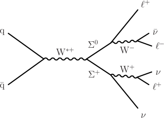
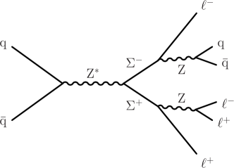
Figure 1: Example processes illustrating production and decay of type-III seesaw heavy fermion pairs at the LHC that result in multilepton final states.

0.2.2 Vector-like leptons

Vector-like fermions are hypothetical particles whose left- and right-handed components transform under conjugate representations of the SM gauge symmetries [delAguila:1982fs, Fishbane:1985gu, Fishbane:1987tx, Montvay:1988av, Fujikawa:1994we], and hence their masses are independent of the SM Higgs mechanism and are not constrained by electroweak precision measurements [delAguila:1989rq, delAguila:2008pw]. Vector-like fermions arise in a wide variety of BSM scenarios, including, but not limited to, supersymmetric models [Martin:2009bg, Graham:2009gy, Endo:2011mc, Zheng:2019kqu], models with extra spatial dimensions [Kong:2010qd, Huang:2012kz], and grand unified theories [Nevzorov:2012hs, Dorsner:2014wva, Joglekar:2016yap]. Extensions of the SM with one or more vector-like fermion families may provide a dark matter candidate [Schwaller:2013hqa, Halverson:2014nwa, Bahrami:2016has, Bhattacharya:2018fus], and account for the mass hierarchy between the different generations of particles in the SM via their mixings with the SM fermions [Agashe:2008fe, Redi:2013pga, Falkowski:2013jya]. Furthermore, vector-like leptons are also among the proposed solutions to the observed tensions between the experimental measurements and the SM prediction of the anomalous magnetic moment of the muon [Endo:2011mc, Dermisek:2013gta, Megias:2017dzd, Kawamura:2019rth, Hiller:2020fbu, Muong-2:2006rrc, Muong-2:2021ojo].

In this paper, we consider two distinct models in which the vector-like leptons couple to the SM lepton [Kumar:2015tna, Bhattiprolu:2019vdu]. The vector-like doublet model contains an SU(2) doublet ($\PGt^{\prime}$,$\PGn^{\prime}$), where the $\PGt^{\prime}$and $\PGn^{\prime}$are mass-degenerate at tree level and can be produced in pairs ($\Pp\Pp\to\PGt^{\prime+}\PGt^{\prime-}/~{}\PGn^{\prime}\Xspace\overline{\PGn^{\prime}\Xspace}$) or in association ($\Pp\Pp\to\PGt^{\prime}\Xspace\PGn^{\prime}\Xspace$). The decay modes are $\PGt^{\prime}\Xspace\to\PZ\Pgt$ or $\PH\Pgt$, and $\PGn^{\prime}\Xspace\to\PW\Pgt$, with the branching fractions of the $\PGt^{\prime}$dependent on the mass $m_{\PGt^{\prime}\Xspace}$. An example of the complete decay chain for the associated production would be $\PGn^{\prime}\Xspace\PGt^{\prime\pm}\to\PW^{\pm}\Pgt^{\mp}\PH\Pgt^{\pm}\to\Pell^{\pm}\Pgn\Pgt^{\mp}b\overline{b}\Pgt^{\pm}$ and for the pair production would be $\PGn^{\prime}\Xspace\overline{\PGn^{\prime}\Xspace}\to\PW^{\pm}\Pgt^{\mp}\PW^{\pm}\Pgt^{\mp}\to\Pell^{\pm}\Pgn\Pgt^{\mp}\Pell^{\pm}\Pgn\Pgt^{\mp}$. In the vector-like singlet model, only a charged lepton ($\PGt^{\prime}$) is present. The $\PGt^{\prime}$can decay to either $\PZ\Pgt$ or $\PH\Pgt$, or $\PW\Pgn$, with the branching fractions similarly governed by $m_{\PGt^{\prime}\Xspace}$. Figure 2 shows two processes from the doublet and singlet models, which exemplify the production and decay of vector-like lepton pairs that result in multilepton final states.

Electroweak precision data constrain the mixing angle between vector-like leptons and SM leptons to be less than about $10^{\mathrm{-2}}$, permitting prompt decays for mass values that are close to the electroweak scale [Dermisek:2014cia, Dermisek:2014qca]. We assume prompt decays of vector-like leptons; aside from this assumption, the analysis is insensitive to the precise values of the mixing angles.

The most stringent constraints on models with vector-like lepton doublets are from a search conducted by the CMS Collaboration [Sirunyan:2019ofn] with 77of data collected in 2016–2017, which excludes them in the mass range of 120–790. The search is performed with multilepton final states consisting of up to four electrons and muons, and also an additional final state with two light leptons along with one hadronically decaying lepton. There are, so far, no direct constraints on the vector-like lepton singlet model from any of the LHC experiments. The L3 Collaboration at the LEP placed a lower bound of $\sim$100on the mass of additional heavy leptons [Achard:2001qw].

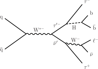
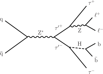
Figure 2: Example processes illustrating production and decay of doublet vector-like lepton pairs at the LHC that result in multilepton final states. The right diagram also illustrates the singlet scenario.

0.2.3 Leptoquarks

Leptoquarks are color-triplet scalar or vector bosons that carry nonzero baryon and lepton quantum numbers and fractional electric charge [Buchmuller:1986zs]. Such particles commonly emerge in grand unified theories, , based on $SU(4)$ [Pati:1974yy], $SU(5)$ [Georgi:1974sy], or $SO(10)$ [Fritzsch:1974nn] schemes, models with compositeness [Gripaios:2014tna, DaRold:2018moy], and R-parity violating supersymmetry models [Weinberg:1981wj, Barbier:2004ez].

In $\Pp\Pp$ collisions at the LHC, scalar leptoquarks (S) could be pair-produced via strong interactions, with the production cross section depending only on the leptoquark mass, $m_{S}$, but not on the unknown Yukawa coupling. Depending on the nature of the Yukawa coupling, such leptoquarks are expected to decay either to an up-type quark and a charged lepton or to a down-type quark and a neutrino, with branching fractions $\beta$ and $1-\beta$, respectively. We assume that the Yukawa couplings involve only one generation of quarks or leptons. The simultaneous coupling of leptoquarks to more than one generation of quarks or leptons that are not aligned with the SM Yukawa couplings may lead to quark or lepton flavor violation [Mandal:2019gff, Diaz:2017lit].

In this analysis, we consider scalar leptoquarks [Davidson:2011zn] with electric charge of $-1/3\abs{e}$, and a nonzero Yukawa coupling to the top quark and a single flavor of SM charged lepton. In a supersymmetric theory, these leptoquarks are right handed down-type squarks that couple to the top quark and charged leptons through leptonic-hadronic R parity violating interactions, where the down-type squarks are the scalar partners of the SM down-type quarks. We assume that only one flavor of charged lepton coupling dominates at a time, and hence consider leptoquark branching fractions $\mathcal{B}_{\Pe}=1$, $\mathcal{B}_{\PGm}=1$, or $\mathcal{B}_{\PGt}=1$, for leptoquarks decaying into a top quark and a charged lepton of the first-, second-, or third-generation, respectively. We target the mass range from just above the top quark mass up to the scale. Furthermore, the leptoquark decays are assumed to be prompt, and the coupling is assumed to satisfy $\lesssim$0.1, within the bounds on such Yukawa couplings from leptonic boson decays [Mizukoshi:1994zy, Davidson:2011zn]. As with the type-III seesaw and vector-like lepton models, the analysis is independent of the magnitude of the leptoquark Yukawa couplings aside from the assumption of prompt decays. Figure 3 shows two processes exemplifying the production and decay of leptoquark pairs that result in multilepton final states.

Leptoquarks with preferential couplings to third-generation fermions have been suggested among the possible extensions of the SM [Alvarez:2018gxs, Angelescu:2018tyl, Crivellin:2019dwb, Saad:2020ucl, Haisch:2020xjd] motivated by a series of anomalies recently observed in charged- and neutral-current B meson decays, $\Pb\to\mathrm{c}\Pell\PGn$ [BaBar:2013mob, Belle:2019rba, LHCb:2017vlu, LHCb:2017smo, LHCb:2021trn] and $\Pb\to\mathrm{s}\Pell\Pell$ [Belle:2016fev, LHCb:2017avl, LHCb:2019hip], respectively. The ATLAS and CMS Collaborations have conducted a number of searches for leptoquarks with flavor-diagonal and cross-generational couplings involving third-generation fermions [Aad:2020jmj, Aad:2021rrh, ATLAS:2019qpq, Sirunyan:2018ruf, CMS:2018svy, Sirunyan:2020zbk, CMS:2018qqq, CMS:2018iye, CMS:2018txo]. The most stringent constraints on scalar leptoquarks with 100% branching fraction to a top quark and first-, second-, or third-generation lepton are set by ATLAS, excluding such particles with masses below 1.48, 1.47 [Aad:2020jmj] and 1.43 [Aad:2021rrh], respectively. Similarly, CMS has excluded scalar leptoquarks decaying to a top quark and a lepton or a bottom quark and a neutrino with equal branching fractions ($\beta=0.5$) with masses below 950 [Sirunyan:2020zbk]. The final states include hadronically decaying top quark and lepton, -tagged jet, and significant missing energy.

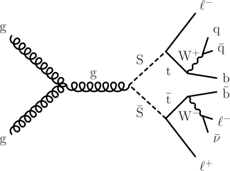
Figure 3: Example processes illustrating the production and decay of scalar leptoquark pairs in $\Pp\Pp$ collisions at the LHC that result in multilepton final states.

0.3 The CMS detector

The central feature of the CMS apparatus is a superconducting solenoid of 6m internal diameter, providing a magnetic field of 3.8T. Within the solenoid volume are a silicon pixel and strip tracker, a lead tungstate crystal electromagnetic calorimeter (ECAL), and a brass and scintillator hadron calorimeter (HCAL), each composed of a barrel and two endcap sections. Forward calorimeters extend the pseudorapidity ($\eta$) coverage provided by the barrel and endcap detectors. Muons are detected in gas-ionization chambers embedded in the steel flux-return yoke outside the solenoid. A more detailed description of the CMS detector, together with a definition of the coordinate system used and the relevant kinematic variables, can be found in Ref. [Chatrchyan:2008zzk].

Events of interest are selected using a two-tiered trigger system. The first level, composed of custom hardware processors, uses information from the calorimeters and muon detectors to select events at a rate of around 100kHz within a fixed latency of about 4 [Sirunyan:2020zal]. The second level, known as the high-level trigger, consists of a farm of processors running a version of the full event reconstruction software optimized for fast processing, and reduces the event rate to around 1kHz before data storage [Khachatryan:2016bia].

0.4 Data samples and event simulation

The total integrated luminosity recorded by CMS in $\Pp\Pp$ collisions at $\sqrt{s}=13\TeV$ corresponds to 138, with 36.3, 41.5, and 59.8recorded in the years 2016, 2017, and 2018, respectively. The data presented here are collected using a combination of isolated single-electron (-muon) triggers with corresponding transverse momentum () thresholds of 27 (24)in 2016, and 32 (27)in 2017, and 32 (24)in 2018. The rates of signal and SM background processes that gives rise to isolated and nondisplaced leptons are estimated from Monte Carlo (MC) simulations, which incorporate detailed detector and $\Pp\Pp$ collision properties.

The $\PZ\PGg$, $\PW\PZ$, $\ttbar\PV$, and triboson ($\PV\PV\PV$) backgrounds, where denotes a or boson, are generated using (versions 2.2.2 for 2016 data and 2.4.2 for 2017 and 2018 data) [Alwall:2014hca] at next-to-leading order (NLO) precision in perturbative quantum chromodynamics (QCD). The top quark mass used in all simulations is 172.5. The $\PZ\PGg$ background includes all diagrams contributing to $\Pp\Pp\to\Pell\Pell\PGg$, with photons from both initial-state radiation (ISR) and final-state radiation (FSR), and with an invariant mass cut of $m(\Pell^{+}\Pell^{-})>10\GeV$. The $\PZ\PZ$ background contribution from quark-antiquark annihilation production is generated using 2.0 [Nason:2004rx, Frixione:2007vw, Alioli:2010xd] at NLO, whereas the contribution from gluon-gluon fusion production is generated at leading order (LO) using 7.0.1 [Campbell:2010ff]. The SM processes involving Higgs boson production are generated using , and JHUGen 7.0.11 [Gao:2010qx, Bolognesi:2012mm, Anderson:2013afp, Gritsan:2016hjl] at NLO, for a Higgs boson mass of 125. Processes with a single top quark and a boson or with four top quarks are simulated using at NLO in QCD. Other small contributions from processes involving a single top quark and an electroweak or Higgs boson, two top quarks and two bosons, or three top quarks are simulated using at LO in QCD. Simulated event samples for the Drell–Yan (DY) and $\ttbar$ processes, which are used for systematic uncertainty studies and in the BDT training process, are generated at NLO with and , respectively.

All signal samples are simulated at LO precision. The type-III seesaw and vector-like lepton samples are generated with  2.6.1, whereas the leptoquark samples are generated with 8.212 (8.230) in 2016 (2017 and 2018) [Sjostrand:2014zea]. The production cross sections for the type-III seesaw signal model are calculated at NLO plus next-to-leading logarithmic precision, assuming that the heavy leptons are SU(2) triplet fermions [Fuks:2012qx, Fuks:2013vua]. Similarly, vector-like lepton and leptoquark cross sections are calculated at NLO precision [Bhattiprolu:2019vdu, Blumlein:1996qp, Kramer:2004df]. In this paper, these higher-order cross sections are used in the analysis of these BSM models.

The NNPDF3.0 LO or NLO parton distribution function (PDF) sets [Ball:2014uwa] are used for all background and signal samples for 2016 data, with order matching that of the matrix element calculations. The NNPDF3.1 next-to-NLO order (NNLO) PDF set [Ball:2017nwa] is used for all 2017 and 2018 samples. To perform the parton showering, fragmentation, and hadronization of the matrix-level events in all samples, 8.212 is used with the event tune CUETP8M1 [Khachatryan:2015pea] for 2016, and 8.230 is used with the event tune CP5 [CMS:2019csb] for 2017 and 2018. The MLM [Hoeche:2006ps] or FxFx [Frederix:2012ps] jet matching schemes are used for samples at LO or NLO, respectively. The simulation of the response of the CMS detector to incoming particles is performed using the $\GEANTfour$ toolkit [Agostinelli:2002hh]. Additional inelastic $\Pp\Pp$ interactions from the same or nearby bunch crossings (pileup) are simulated and incorporated in the MC samples.

0.5 Event reconstruction and particle identification

In each event, the candidate vertex with the largest total physics-object $\pt^{2}$ is taken to be the primary $\Pp\Pp$ interaction vertex (PV). The physics objects are the jets, clustered using the anti-algorithm [Cacciari:2008gp, Cacciari:2011ma] with the tracks assigned to candidate vertices as inputs, and the associated , which is the negative vector sum of those jets.

The reconstruction and identification of individual particles in an event is based on the particle-flow (PF) algorithm [Sirunyan:2017ulk], with an optimized combination of information from the various elements of the CMS detector. The energy of photons is obtained from the ECAL measurement. The energy of electrons is determined from the electron momentum at the PV as determined by the tracker, the energy of the corresponding ECAL cluster, and the energy sum of all bremsstrahlung photons spatially compatible with originating from the electron track. The momentum of muons is determined from the curvature of the corresponding track, and the energy is obtained from the momentum. The energy of charged hadrons is determined from a combination of their momentum measured in the tracker and the matching ECAL and HCAL energy deposits, corrected for the response function of the calorimeters to hadronic showers. Finally, the energy of neutral hadrons is obtained from the corresponding corrected ECAL and HCAL energies.

Electrons are reconstructed by geometrically matching charged-particle tracks from the tracking system with energy clusters deposited in the ECAL [CMS:2020uim]. The electron momentum is estimated by combining the energy measurement in the ECAL with the momentum measurement in the tracker. The momentum resolution for electrons with $\pt\approx 45\GeV$ from $\PZ\to\Pe\Pe$ decays ranges from 1.7 to 4.5%. It is generally better in the barrel region than in the endcaps, and also depends on the bremsstrahlung energy emitted by the electron as it traverses the material in front of the ECAL. To suppress undesired electrons originating from photon conversions in detector material, as well as the misidentification of hadrons, the electron candidates are required to satisfy shower shape and track quality requirements, using the medium cut-based criteria described in Ref. [CMS:2020uim]. Electrons used in this analysis are also required to satisfy $\pt>10\GeV$ and $\abs{\eta}<2.4$.

Muons are reconstructed from compatible tracks in the inner tracker and the muon detectors [Sirunyan:2018fpa]. Additional track fit and matching quality criteria suppress the misidentification of hadronic showers that punch through the calorimeters and reach the muon system. Matching tracks measured in the inner tracker and the muon detectors results in a relative resolution, for muons with up to 100, of 1% in the barrel and 3% in the endcaps, and of better than 7% in the barrel for muons with up to 1 [Sirunyan:2018fpa]. Muons used in this analysis must lie within the tracking system acceptance, $\abs{\eta}<2.4$, and are required to have $\pt>10\GeV$.

Hadronically decaying lepton candidates () are reconstructed from jets, using the hadrons-plus-strips algorithm [Sirunyan:2018pgf], which combines one or three tracks with energy deposits in the calorimeters, to identify the corresponding one- or three-prong lepton decay modes. Neutral pions from lepton decay are reconstructed as strips with variable size in $\eta$-$\phi$ from reconstructed electrons and photons, where the $\phi$ is azimuthal angle in radians and the strip size varies as a function of the of the electron or photon candidate. The reconstructed candidate must satisfy $\abs{\eta}<2.3$ and $\pt>20\GeV$.

Jets are clustered using the anti-algorithm [Cacciari:2008gp] with a distance parameter of 0.4, as implemented in the FastJet package [Cacciari:2011ma]. The minimum threshold for the jets selected in this analysis is 30and the central axis of the jet is also required to be inside the tracking acceptance, $\abs{\eta}<2.4$. Jets are composite objects made up of several particles, hence the momentum is determined as the vectorial sum of all particle momenta, and is found from simulation to be, on average, within 5–10% of the true momentum over the whole spectrum and detector acceptance. Additional $\Pp\Pp$ interactions within the same or nearby bunch crossings can contribute additional tracks and calorimetric energy depositions, increasing the apparent jet momentum. To mitigate the effect of the charged-particle contribution from pileup on reconstructed jets, a charged hadron subtraction technique is employed, which removes the energy of charged hadrons not originating from the PV [Sirunyan:2017ulk]. In addition, the impact of neutral pileup particles in jets is mitigated by an event-by-event jet-area-based correction of the jet four-momenta [Cacciari:2008ca, Cacciari:2008ps, Sirunyan:2017jes]. Aside from pileup contamination removal, additional quality criteria are applied to each jet to remove those potentially mismeasured because of instrumental effects or reconstruction failures [CMS:2017jme]. Finally, the qualifying jets must lie outside a cone of $\Delta R\equiv\sqrt{\smash[b]{(\Delta\eta)^{2}+(\Delta\phi)^{2}}}=0.4$ around a selected muon, electron, or candidate, where $\Delta\phi$ is the $\phi$ angle between the jet and lepton.

Jet energy corrections are derived from simulation studies so that the average measured energy of jets matches that of particle level jets. In situ measurements of the balance in dijet, photon+jet, leptonically decaying $\PZ$+jet, and multijet events are used to determine any residual differences between the jet energy scale in data and in simulation, and appropriate corrections are made to the jet  [Sirunyan:2017jes].

The reconstructed jets originating from hadrons are identified using the medium working point of the DeepCSV tagging algorithm [Sirunyan:2017ezt]. This working point has an identification efficiency of 60–75% for quark jets, depending on jet and $\eta$, and a misidentification probability of about 10% for quark jets and about 1% for light-quark and gluon jets.

The vector is defined as the negative vector sum of all the PF candidates in an event, and its magnitude is denoted as  [Sirunyan:2019kia]. The pileup-per-particle identification algorithm [Bertolini:2014bba] is applied to reduce the pileup dependence of the observable. The is computed from the PF candidates weighted by their probability to originate from the PV, and is modified to account for corrections to the energy scale of the reconstructed jets in the event.

The leptons that are produced from the decays of the SM bosons , , (either directly, or via an intermediate lepton) are referred to as prompt leptons, and are often indistinguishable in momentum and isolation from those produced in signal events. Thus, the SM processes giving rise to three or more isolated leptons, such as $\PW\PZ$, $\PZ\PZ$, $\ttbar\PV$, $\PV\PV\PV$, and Higgs boson production, constitute the irreducible backgrounds in this analysis. On the other hand, reducible backgrounds come from SM processes in which the jets are misidentified as leptons, or where the leptons originate from heavy-quark decays. Some examples of such backgrounds are $\PZ$+jets or $\ttbar$+jets production, in which the prompt leptons are accompanied by leptons that are within or near jets, hadrons that traverse the HCAL and reach the muon detectors, or hadronic showers with large electromagnetic energy fractions. Leptons from such sources are referred to as misidentified leptons, and SM background processes with such misidentified leptons are collectively labeled as “MisID” backgrounds in the subsequent discussion.

The reducible backgrounds are significantly suppressed by applying stringent requirements on the lepton isolation and displacement. For electron and muon candidates, the relative isolation is defined as the scalar sum, normalized to the lepton , of photon and hadron PF objects within a cone of radius $\Delta R$ around the lepton. For electrons, the relative isolation is required to be less than $0.0478+0.506\GeV/\pt$ in the barrel ($\abs{\eta}<1.479$) and less than $0.0658+0.963\GeV/\pt$ in the endcap ($\abs{\eta}>1.479$), with $\Delta R=0.3$. The relative isolation for muons is required to be less than 0.15 with $\Delta R=0.4$. The isolation quantities are also corrected for contributions from particles originating from pileup vertices. In addition to the isolation requirement, electrons in the barrel must satisfy $\abs{d_{\mathrm{z}}}<0.1\cm$ and $\abs{d_{\mathrm{xy}}}<0.05\cm$, and in the endcap $\abs{d_{\mathrm{z}}}<0.2\cm$ and $\abs{d_{\mathrm{xy}}}<0.1\cm$, where $d_{\mathrm{z}}$ and $d_{\mathrm{xy}}$ are the longitudinal and transverse impact parameters of electrons with respect to the PV, respectively. Similarly, muons must satisfy $\abs{d_{\mathrm{z}}}<0.1\cm$ and $\abs{d_{\mathrm{xy}}}<0.05\cm$. For both electrons and muons, the three-dimensional impact parameter significance, the impact parameter value divided by its uncertainty, must be less than 10, 12, and 9 in 2016, 2017, and 2018 data, respectively. All selected electrons within a cone of $\Delta R<0.05$ of a selected muon are discarded in order to reduce bremsstrahlung contributions from muons.

For leptons, the DeepTau [TAU-20-001] algorithm is used to distinguish genuine hadronic tau lepton decays from jets originating from the hadronization of quarks or gluons, as well as from electrons or muons. Information from all individual reconstructed particles near the axis is combined with properties of the candidate and the event. In addition to this multivariate requirement, candidates must satisfy $\abs{d_{\mathrm{z}}}<0.2\cm$. All selected candidates within a cone of $\Delta R<0.5$ of a selected electron or muon are also discarded to suppress misidentified tau leptons.

Additionally, to suppress misidentified leptons originating from heavy-flavor decays, leptons are discarded if a -tagged jet with $\pt>10\GeV$ and $\abs{\eta}<2.5$ is found within a cone of radius $\Delta R<0.4$ around the lepton.

These lepton reconstruction and selection requirements result in typical efficiencies of 40–85%, 65–90%, and 20–50% for electrons, muons, and leptons, respectively, depending on lepton and $\eta$.

0.6 Event selection

We consider seven distinct final states (channels) based on the number of light leptons and candidates. These seven channels are orthogonal, and are defined as:

• $\geq$4 light leptons and any number of candidates (4L),

• exactly 3 light leptons and $\geq$1 candidates (3L1T),

• exactly 3 light leptons and no candidates (3L),

• exactly 2 light leptons and $\geq$2 candidates (2L2T),

• exactly 2 light leptons and exactly 1 candidates (2L1T),

• exactly 1 light lepton and $\geq$3 candidates (1L3T), and

• exactly 1 light lepton and exactly 2 candidates (1L2T).

In the 4L channel, only the leading four light leptons in are used in the subsequent analysis. Likewise, in the 3L1T, 2L2T, and 1L3T channels, only the leading 1, 2, and 3 candidates are used, respectively. In each channel, at least one muon with $>$ 26 (29)in 2016 and 2018 (2017) or at least one electron with $>$ 30 (35)in 2016 (2017 and 2018) is required, with the thresholds set in order to be consistent with the triggers used.

The events in these seven channels are further classified based on several event properties. This classification is used to enhance sensitivity to particular signal decay chains, or to define dedicated selections to help constrain the SM backgrounds. The quantities are defined below.

• Scalar momentum sums: We define $L_{\mathrm{T}}$ as the scalar sum of all charged leptons that constitute the channel. For example, in the 4L channel, $L_{\mathrm{T}}$ is calculated from the leading four light leptons in , while for the 3L1T channel, it is calculated from the three light leptons and the leading . We define $\HT$ as the scalar sum of all jets. Additionally, the scalar sum of $L_{\mathrm{T}}$, $\HT$, and is defined as $S_{\mathrm{T}}$. The quantity $L_{\mathrm{T}}$+$\ptmiss$ is also of interest. For the signal models considered in this analysis, high signal mass hypotheses give rise to events with high $L_{\mathrm{T}}$, $\HT$, , and $S_{\mathrm{T}}$.

• Charge and flavor combinations: We count the number OSSF$n$ as distinct opposite-sign (electric charge) same-flavor lepton pairs in an event. Specific lepton pairs are labeled as OSSF (opposite-sign, same-flavor) and OSDF (opposite-sign, different-flavor). We define $Q_{\Pell}$ as the sum of charges of all leptons in the event.

• Invariant and transverse masses: We define $M_{\Pell}$ as the invariant mass of all leptons in the event, and $M_{\text{min}}$ as the minimum invariant mass of all dilepton pairs in the event, irrespective of charge or flavor. Additionally, the invariant mass of leptons $i$ and $j$ is defined as $M^{\mathrm{ij}}$. The transverse mass for a single lepton $i$ is defined as $M_{\mathrm{T}}^{\mathrm{i}}=(2\ptmiss\pt^{\mathrm{i}}[1-\text{cos}(\vec{p}_{\mathrm{T}}^{\text{miss}},\ptvec^{\mathrm{i}})])^{\mathrm{1/2}}$, where $\pt^{\mathrm{i}}$ is the of lepton $i$. Similarly, $M_{\mathrm{T}}^{\mathrm{ij}}$ is defined as the transverse mass calculated with the and the resultant 4-momentum sum of lepton $i$ and $j$. The lepton indices run over up to 4 leptons, in descending order.

  We define the $M_{\text{OSSF}}$ variable in a given event as the OSSF dielectron or dimuon mass closest to the boson mass at $91\GeV$ [Zyla:2020zbs], subject to some additional constraints, and label events with $M_{\text{OSSF}}$ within 15of the boson mass (76–106mass window) as OnZ. Throughout this paper, OSSF1 or OSSF2 events that are not OnZ are labeled as OffZ. In the 3L event with a distinct OSSF pair (such as in $\Pe^{+}\Pe^{-}\PGm^{+}$, $\PGm^{+}\PGm^{-}\Pe^{-}$), the event is classified as BelowZ, OnZ, or AboveZ if the $M_{\text{OSSF}}<76\GeV$, within 76–106, or $>$106, respectively. In the 3L events with two nondistinct OSSF pairs (such as in $\Pe^{+}\Pe^{-}\Pe^{+}$), the events are classified as OnZ if either pair satisfies $M_{\text{OSSF}}$ within 76–106, as BelowZ if both pairs have masses $<$76, or as AboveZ if both pairs have masses $>$106. In cases where one pair has mass $<$76and the other pair has mass $>$106, the event is classified as MixedZ.

  In 3L OSSF1 events, the $M_{\mathrm{T}}$ variable is defined as $M_{\mathrm{T}}^{\mathrm{i}}$, where the lepton $i$ is not part of the $M_{\text{OSSF}}$ pair. In events with three electrons or three muons, the $M_{\text{OSSF}}$ and $M_{\mathrm{T}}$ variables are chosen simultaneously so that the event is OnZ, and $M_{\mathrm{T}}$ is in the range 50–150, where this is kinematically possible. Similarly, in 4L OSSF2 events with four electrons or muons, $M_{\text{OSSF}}$ is chosen to give the maximum number of nonoverlapping OSSF pairs with masses within the boson mass window. Such events are labeled as Single- or Double-OnZ, respectively, depending on whether they have one or two nonoverlapping OnZ OSSF pairs. Additionally, the of the $M_{\text{OSSF}}$ lepton pair is defined as $\pt^{\text{OSSF}}$.

  The signal models and the SM backgrounds can have multiple and bosons in the decay chains. The invariant and transverse mass quantities aid in defining regions to isolate these specific decays. The $M_{\text{OSSF}}$ and $M_{\mathrm{T}}$ variables primarily isolate events with $\PZ\to\Pell\Pell$ and $\PW\to\Pell\PGn$ decays, respectively, while $M_{\mathrm{T}}^{\mathrm{ij}}$ is useful in describing signal events with two visible leptons and , such as $\PGn^{\prime}\Xspace\to\PW\PGt\to\Pell\PGt\PGn$ in the vector-like lepton doublet model.

• Angular quantities: We define $\Delta{R}_{\text{min}}$ as the minimum $\Delta{R}$ between all the dilepton pairings in an event, irrespective of charge or flavor. Similarly, $\Delta{R}_{\text{min}}^{\tauh}$ is defined as the minimum $\Delta{R}$ between any dilepton pair, where at least one of the leptons is a candidate. The quantities $\Delta\phi^{\mathrm{ij}}$ and $\Delta\eta^{\mathrm{ij}}$ are defined as the azimuthal angle or pseudorapidity difference between the $i^{\mathrm{th}}$ and $j^{\mathrm{th}}$ lepton, whereas $\Delta\phi^{\mathrm{i}}$ is defined to denote the opening azimuthal angle between lepton $i$ and . These are quantities that help to characterize the topology of the signal and background events.

• Counts: We define $N_{\mathrm{j}}$ as the multiplicity of jets and $N_{\PQb}$ as the multiplicity of -tagged jets satisfying the selection criteria defined earlier.

Finally, all events with $M_{\text{min}}<12\GeV$, $\Delta{R}_{\text{min}}<0.2$, or $\Delta{R}_{\text{min}}^{\tauh}<0.5$ are vetoed in order to suppress contributions due to low-mass resonances (, ) and low-$\Delta{R}$ FSR photons.

0.7 Background estimation

A set of control regions (CRs) dominated by the primary background processes is used for the purpose of SM background determination. A summary of all the CR definitions is provided in Table 0.7. These CRs are utilized to develop and verify a mixture of methods based on both MC simulations and data: normalizing simulated samples for the dominant irreducible SM processes, deriving any residual corrections to the simulated samples, and developing the background estimates based on data for the reducible background contributions. The CRs consist of the following selections: 4L events with two OSSF OnZ pairs and no  jets (4L $\PZ\PZ$ CR); 3L events with an OSSF OnZ pair, $M_{\mathrm{T}}<150\GeV$, and $\ptmiss<125\GeV$ (3L OnZ CR); 3L OffZ events with a trilepton mass OnZ and no  jets (3L $\PZ\PGg$ CR); and 2L1T events with an OSSF OnZ pair and $\ptmiss<100\GeV$ (2L1T MisID CR). The 3L OnZ CR is further split into three subregions with the following criteria: $\ptmiss<100\GeV$, $M_{\mathrm{T}}<50\GeV$, and $N_{\PQb}=0$ (3L MisID $\Pe/\PGm$ CR); $50<M_{\mathrm{T}}<150\GeV$, minimum lepton $\pt>20\GeV$, and $N_{\PQb}=0$ (3L $\PW\PZ$ CR); and $\ptmiss<125\GeV$, $M_{\mathrm{T}}<150\GeV$, minimum lepton $\pt>20\GeV$, $N_{\PQb}>0$, $N_{\mathrm{j}}>2$, and $S_{\mathrm{T}}>350\GeV$ (3L $\ttbar\PZ$ CR). Events satisfying any of the CR selection criteria are not considered in the SRs.

A summary of control regions for the irreducible SM processes $\PZ\PGg$, $\PW\PZ$, $\ttbar\PZ$, and $\PZ\PZ$, and for the misidentified lepton backgrounds. The , $M_{\mathrm{T}}$, the minimum 3L lepton $(\pt^{\mathrm{3}})$, and $S_{\mathrm{T}}$ are in units of . The 3L OnZ CR is further split into 3L MisID $\Pe/\PGm$ CR, 3L $\PW\PZ$ CR, and 3L $\ttbar\PZ$ CR. l l l r r r r l CR name & OSSF$n$ $M_{\text{OSSF}}$ $N_{\PQb}$ $M_{\mathrm{T}}$ $\pt^{\mathrm{3}}$ Other selections
2L1T MisID OSSF1 OnZ $<$100
3L $\PZ\PGg$ OSSF1 BelowZ 0 Trilepton mass OnZ
3L OnZ OSSF1 OnZ $<$125 $<$150
3L MisID $\Pe/\PGm$ OSSF1 OnZ 0 $<$100 $<$50
3L $\PW\PZ$ OSSF1 OnZ 0 $<$125 50–150 $>$20
3L $\ttbar\PZ$ OSSF1 OnZ $\geq$1 $<$125 $<$150 $>$20 $N_{\mathrm{j}}>2$, $S_{\mathrm{T}}>350$
4L $\PZ\PZ$ OSSF2 Double-OnZ 0

0.7.1 Irreducible backgrounds

The irreducible backgrounds, as described earlier, arise from processes in which all reconstructed leptons originate from decays of SM bosons. These contributions are estimated using simulated event samples, after normalization and validation in dedicated CRs in data for the major $\PW\PZ$, $\PZ\PZ$, $\PZ\PGg$, and $\ttbar\PZ$ processes. The normalization correction factors and associated uncertainties, which include both statistical and systematic contributions, take into account the contamination of events from other processes, and are applied to the corresponding background estimates in the SRs. The measurements for the diboson processes are largely independent because of the high purity of the corresponding CRs. Since these backgrounds make significant contributions to the $\ttbar\PZ$-enriched CR, the normalization correction for this process is measured after the corresponding corrections have been obtained for the other backgrounds.

The $\PZ\PZ\to 4\Pell$ process is the primary background component in the channels with four leptons. The fraction of $\PZ\PZ$ events in the 4L $\PZ\PZ$ CR is greater than 99%. We consider the $\PQq\PQq\to\PZ\PZ\to 4\Pell$ and $\Pg\Pg\to\PZ\PZ\to 4\Pell$ processes collectively, and observe relative normalization uncertainties of 4–5% in each of the three data-taking periods. These uncertainties are dominated by the statistical uncertainties, as the contamination from background processes other than $\PZ\PZ$ is negligible in this CR.

The $\PW\PZ\to 3\Pell\PGn$ process is the primary irreducible background source for channels with three leptons. This background is normalized to data in the 3L $\PW\PZ$ CR, where the minimum lepton threshold is raised to 20to suppress the misidentified lepton contributions, and the selection yields a set of events $>75\%$ pure in $\PW\PZ$. We observe relative normalization uncertainties in the range 3–6% across the three data-taking periods for the $\PW\PZ\to 3\Pell\PGn$ process, which include the statistical and systematic components due to subtraction of background processes other than $\PW\PZ$.

The $\PZ\PZ$ and $\PW\PZ$ simulation samples are reweighted as functions of the jet multiplicity as well as the visible diboson to match the simulated distributions to those of the data in these CRs, where the visible diboson is defined as the vector sum of the charged leptons in the event. This accounts for missing higher-order QCD and electroweak corrections, and yields an improved description of leptonic and hadronic quantities of interest in this analysis.

Production of $\ttbar\PZ$ is a major irreducible SM background process for all channels with $N_{\PQb}>0$. This background is normalized to data in the 3L $\ttbar\PZ$ CR selection, which is orthogonal to the 3L $\PW\PZ$ CR and the misidentified lepton CR selections. Similarly to the selection in the 3L $\PW\PZ$ CR, the minimum lepton threshold is raised to 20to suppress the misidentified lepton contributions, and the selection yields a set of events $\sim$60% pure in $\ttbar\PZ$. Including the statistical and systematic uncertainties due to subtraction of other background processes, we measure relative normalization uncertainties in the range of 20–30% across the three data-taking periods for the $\ttbar\PZ$ process.

A smaller background contribution arises from ISR or FSR photons that convert asymmetrically such that only one of the resultant leptons is reconstructed in the detector, or from misidentifying on-shell photons as electrons. The dominant source of such backgrounds, collectively referred to as the conversion background, is DY events with an additional photon.The cross section of this process is normalized in a dedicated 3L $\PZ\PGg$ CR, consisting of BelowZ trilepton events with $N_{\PQb}=0$, where the mass of the trilepton system is within 15of the boson mass. The CR targets $\PZ\to\Pell\Pell+\PGg$ events, where, for example, the photon converts in the detector and one of the four leptons is too soft to satisfy our lepton selection criteria. This selection yields a set of events $>70\%$ pure in $\PZ\PGg$. We obtain relative normalization uncertainties of about 10% across the three data-taking periods, where the quoted value includes the statistical and systematic components due to subtraction of background processes other than $\PZ\PGg$, as well as a flavor-dependent component due to varying fractions of internal and external conversions as a function of electron multiplicity in the events.

Other irreducible processes that are not normalized in a dedicated CR in data are estimated from simulation samples and normalized to their theoretical cross sections.

In the following figures, diboson backgrounds from $\PW\PZ$ and $\PZ\PZ$ processes are denoted as “$\PV\PV$”, whereas the $\ttbar\PZ$ and $\ttbar\PW$ contributions are labeled as “$\ttbar\PV$”. Background processes involving a lepton conversion, particularly the $\PZ\PGg$ process, are labeled as “Conv.” Other irreducible backgrounds estimated using simulation consist of triboson, Higgs boson, and other rare SM contributions, and are collectively referred to as “Rare” backgrounds.

0.7.2 Misidentified lepton backgrounds

The misidentified lepton backgrounds are estimated via a three- or four-dimensional implementation of a matrix method [Khachatryan:2015bsa], based on the lepton multiplicity in the targeted signal selections in data. The matrix method defines a set of sideband regions for each SR based on the isolation properties of the selected lepton objects in each event. Leptons in the SR selections satisfy the tight lepton definitions given in Section 0.5, whereas the sideband selections are defined by loose criteria with relaxed isolation requirements ($<$1.0 relative isolation for electrons and muons, and a relaxed working point of the DeepTau algorithm for ), but are otherwise identical to the tight lepton criteria. Therefore, for a 3 (4) lepton event in an SR, the matrix method uses an additional 7 (15) nonoverlapping sideband regions with at least one lepton failing the tight isolation criteria. The sideband regions are therefore orthogonal to the SRs by construction. The probabilities with which prompt- and misidentified lepton candidates pass the tight selection, given that they satisfy the loose selection, are denoted as prompt and misidentification rates, respectively. These are measured as a function of various kinematic features of leptons and hadronic properties of events that impact the lepton isolation. These rates are used in the extrapolation from the sideband regions to the SR. This extrapolation is performed for each event, where the contamination due to prompt leptons that fail the tight lepton selection criteria is also corrected for. Because of the isolation requirements used in the single-lepton triggers, background contributions with up to 2 (3) simultaneous misidentified leptons in 3 (4) lepton events can be predicted by this implementation of the matrix method. The fraction of signal events where all lepton candidates are misidentified is found to be negligible in simulation based studies.

The prompt rates are measured using a “tag-and-probe” method [CMS:2011aa] in various dilepton event selections. In data, prompt rates for electrons and muons are studied in a DY-enriched OnZ OSSF $\Pe\Pe$ and $\PGm\PGm$ events, respectively. Similarly, prompt rates for candidates are studied in a DY-enriched set of opposite-sign $\Pe\tauh$ and $\PGm\tauh$ events. In simulation, the prompt rates are measured in DY and $\ttbar$ MC samples, using reconstructed leptons kinematically matched to generator-level prompt leptons ($\Delta{R}<0.2$). The measured prompt rates are primarily parametrized as a function of the lepton and $\abs{\eta}$. Prompt rates for electrons and muons vary from about $65\%$ at $\pt\sim 10\GeV$ to about $95\%$ at $40\GeV$ and above. For one- (three-) prong candidates, the prompt rates are about 50–70% (30–70%) in the range of 20–50. The final prompt rates for all lepton flavors are based on the DY-enriched data measurements, and the differences between rates derived from DY and $\ttbar$ MC simulations are taken as an estimate of the associated systematic uncertainty, accounting for the dependence of prompt rates on hadronic activity. Prompt rate uncertainties are found to be unimportant in the matrix method, and the corresponding impact on the misidentified lepton background estimate is negligible.

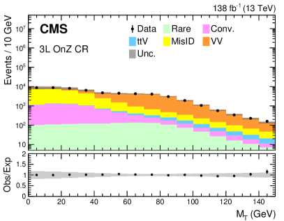
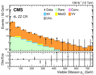
Figure 4: The distributions of $M_{\mathrm{T}}$ in 3L OnZ CR (upper left), visible diboson in 4L $\PZ\PZ$ CR (upper right), in 2L1T MisID CR (lower left), and $\HT$ in 3L $\ttbar\PZ$ CR (lower right) events. The rightmost bin contains the overflow events in each distribution. The lower panel shows the ratio of observed events to the total expected background prediction. The gray band on the ratio represents the sum of statistical and systematic uncertainties in the SM background prediction.

The DY+jets and $\ttbar$+jets processes are the dominant SM contributions to the total misidentified lepton background in multilepton events. However, different gluon, light quark, and heavy quark compositions, as well as different event kinematic properties of these two processes, yield misidentification rates that may differ by up to $50\%$ from each other for a given lepton flavor. Therefore, dedicated data and MC measurements are performed for both processes. A variant of the tag-and-probe method is used for the measurement of the misidentification rates. In both 3L and 2L1T MisID CRs, the OnZ leptons are taken as the tag leptons, and the additional lepton is taken as the misidentified lepton probe, , $\Pe\Pe\Pgm$ and $\Pgm\Pgm\Pgm$ events are used to measure muon misidentification rates, while $\Pe\Pe\tauh$ and $\Pgm\Pgm\tauh$ events are used to measure the misidentification rates. In measurements conducted in data, contributions due to prompt probe leptons are estimated and subtracted using MC simulation. Misidentification rates obtained in simulated $\ttbar$+jets samples are verified in dedicated data CRs enriched in such contributions, where one lepton is required to fail the three-dimensional impact parameter significance requirement or the tag veto described in Section 0.5.

The lepton misidentification rates are also parametrized as functions of the lepton and $\abs{\eta}$. The rates are further split for one- and three-prong objects. The central value of the misidentification rates for each lepton flavor is corrected for the recoil of the event, where the recoil is defined as a function of the vector sum of the of all other leptons, jets, and in the event. These recoil-based corrections improve the modeling of misidentified lepton backgrounds in DY+jets events, in which the misidentified lepton often originates from a jet recoiling against the leptonically decaying boson system. Similarly, the misidentification rates are corrected as a function of the multiplicity of tracks originating from the PV and the jet multiplicity.

The final misidentification rates for all lepton flavors are obtained by a weighted average of the DY- and $\ttbar$-based measurements. These are evaluated according to the expected DY-$\ttbar$ composition of the MisID background, as obtained from simulated samples in each SR category and for each -tagged jet multiplicity. These DY and $\ttbar$ MC samples use normalization factors measured in dedicated dilepton control regions. Half of the difference between rates derived from DY- and $\ttbar$-based measurements is assigned as a systematic uncertainty to allow for inaccurate modeling of the expected background composition. Typical electron and muon misidentification rates, relative to the loose selection, are in the range of 5–30%, whereas those of objects are found to be in the range of 1–15%.

Figure 4 shows a selection of kinematic distributions in the various control regions, with the sum of statistical and systematic uncertainties in the SM background prediction, as described in Section LABEL:sec:systematics. The data are observed to be in agreement with the SM prediction.

0.8 Signal regions

The multilepton events that have been selected in the seven channels following the description in Sections 0.5 and 0.6 are now categorized into two alternative SRs. This categorization is done either in a model-independent way, based on the characteristics of the SM backgrounds, or in a model-dependent way, based on the output of BDTs trained specifically for particular signal hypotheses.

Figure 5 illustrates $L_{\mathrm{T}}$, , and $\HT$ distributions in the full multilepton phase space, and the $M_{\text{OSSF}}$ distribution in channels with at least one OSSF light lepton pair. In each distribution, a benchmark signal hypothesis distribution is overlaid to allow a comparison of shapes between signal and background. The plots include the sum of statistical and systematic uncertainties in the SM background prediction, as described in Section LABEL:sec:systematics, and the data are found to be in agreement with the SM prediction.

Figure 5: The distributions of $L_{\mathrm{T}}$ (upper left), (upper right), and $\HT$ (lower left) in all seven multilepton channels, and $M_{\text{OSSF}}$ (lower right) in channels with at least one light lepton pair (4L, 3L1T, 3L, 2L2T, and 2L1T). The rightmost bin contains the overflow events in each distribution. The lower panel shows the ratio of observed events to the total expected background prediction. The gray band on the ratio represents the sum of statistical and systematic uncertainties in the SM background prediction. As illustrative examples, a signal hypothesis for the production of the vector-like lepton in the doublet scenario of $m_{\PGt^{\prime}\Xspace}=1\TeV$ and a scalar leptoquark coupled to a top quark and a lepton of $m_{{\HepParticle{S}{}{}}\Xspace}=1\TeV$ are overlaid in the $L_{\mathrm{T}}$ and $\HT$ distributions respectively. Similarly, a signal hypothesis for the production of the type-III seesaw heavy fermions in the flavor-democratic scenario of $m_{\Sigma}=1\TeV$ is overlaid for the and $M_{\text{OSSF}}$ distributions.

0.8.1 Model-independent selections

The model-independent SRs are defined by splitting the channels into various lepton charge and flavor combinations, mass variables, and kinematic regions depending on the dominant SM background processes. This categorization allows the complete utilization of multilepton events collected, such that any event that does not populate a CR contributes to an SR. Explicitly, events selected for the CRs, which are used in the estimation of major SM backgrounds as described in Section 0.7, are not used in any of the SRs.

The SRs are designed to separate regions where signs of BSM models could appear from regions dominant in SM background processes. The most easily distinguishable feature is the presence of a boson candidate, determined using OSSF$n$ and $M_{\text{OSSF}}$. The $\PZ\PZ$ and the $\PW\PZ$ processes can be separated by additional requirements on $M_{\mathrm{T}}$ in the event. Similarly, the MisID background can be separated using the minimum lepton . Further selections on $N_{\PQb}$ give SR regions that have significant contributions from $\ttbar\PZ$.

Fundamental scheme of event categorization, as a function of lepton charge combinations and mass variables. The mass categorizations refer to masses of OSSF pairs if present, and of OSDF pairs otherwise, as explained in the text. For categorization purposes, all possible opposite-sign dielectron and dimuon pair masses in the event are considered, whereas only the largest mass in the event is considered for all other opposite-sign pairs. Only the dielectron and dimuon pairs are considered to tag events as OnZ. The 1L3T OSSF0 and OSSF1 events are combined into a single category. Disallowed categories are marked with “”. l l c l l l c l l l l c l l l c   OSSF0   OSSF1   OSSF2
BelowZ AboveZ SS OnZ BelowZ AboveZ MixedZ Single-OnZ Double-OnZ OffZ
3L Low $\pt/M_{\mathrm{T}}$ A1 A1 A2 A3 A4 A5 A6
High $\pt/M_{\mathrm{T}}$ A7 A7 A8 A9 A10 A11 A12
2L1T Low B1 B2 B3 B4 B5 B6
High B7 B8 B9 B10 B11 B12
1L2T C1 C2 C3 C4 C5
4L D1 D1 D1 D2 D3 D3 D3 D4 D5 D6
3L1T E1 E1 E1 E2 E3 E3 E3
2L2T F1 F1 F1 F2 F2 F2 F3 F4
1L3T G1 G1 G1 G1 G1

Based on the idea of the broad categorization described above, we have a fundamental scheme with 43 orthogonal selections labeled A1–G1, as summarized in Table 0.8.1. The primary classification is done based on OSSF$n$, with $n$ being 2, 1, or 0. We also define another scheme, labeled the advanced scheme, which builds on the fundamental scheme, but adds further categories. Each of the 43 fundamental scheme categories is first split into up to three tag multiplicity regions. The categories with 0 tag, 1 tag, and 2 or more tag multiplicities are denoted by 0, 1, and 2respectively, in all the subsequent tables and figures. Furthermore, each category in a given tag multiplicity region is split in up to four bins, using a binary low/high criterion and an $\HT$ requirement. This results in a total of 204 orthogonal categories.

Events where an OSSF light lepton pair is not found, but an OSSF $\PGt\PGt$ pair is found, are categorized as BelowZ or AboveZ with respect to the pole mass ($91\GeV$) using the $\PGt\PGt$ pair mass. This is done since a resonance will not appear at the pole mass because of the neutrino emitted in the lepton decays. In OSSF0 events, an OSDF pair is sought, and the event is categorized as BelowZ or AboveZ (as for $\PGt\PGt$ events) based on the OSDF pair with the largest mass. Events with no OSSF or OSDF pairs are classified as same-sign (SS) events.

The 3L channel is further split into two categories, based on the value of either $M_{\mathrm{T}}$ or the minimum lepton . In the 3L OnZ channel, an $M_{\mathrm{T}}>125\GeV$ criterion is used for a binary low or high classification, whereas a lepton $\pt>25\GeV$ criterion is used for the rest of the 3L channel. The 2L1T channel is split into a similar binary classification based on the candidate $\pt>50\GeV$ criterion.

In order to be sensitive to a large class of BSM models in each of the 43 categories of the fundamental scheme, an $L_{\mathrm{T}}$+$\ptmiss$ distribution is obtained in $200\GeV$ wide bins, with the last bin being inclusive for all higher values. This results in 156 $L_{\mathrm{T}}$+$\ptmiss$ bins. The combined spectrum (across all 43 categories) gives the fundamental $L_{\mathrm{T}}$+$\ptmiss$ table. The width of bins in the spectrum is chosen to provide smooth and monotonic expected background behavior, while still retaining sensitivity to nonresonant models. The first and last bins of the $L_{\mathrm{T}}$+$\ptmiss$ distribution are chosen with the requirement that the per-bin expected background yield is more than 0.5 events to ensure robustness in statistical interpretations.

The second table, labeled the fundamental $S_{\mathrm{T}}$ table, is identical to the first table except that we use the $S_{\mathrm{T}}$ distribution in each category, where $S_{\mathrm{T}}$ is the scalar sum of $L_{\mathrm{T}}$, $\HT$, and , also in $200\GeV$ wide bins, resulting in 257 bins. This table provides sensitivity to signal models with energetic jets, such as leptoquarks, whereas the $L_{\mathrm{T}}$+$\ptmiss$ table is optimized for models without significant hadronic activity, such as vector-like lepton and type-III seesaw scenarios.

For the third and final table, we use $S_{\mathrm{T}}$ as the final discriminating variable, binned in $200\GeV$ increments, in the advanced scheme categorization resulting in 805 bins. This table, labeled the advanced $S_{\mathrm{T}}$ table, provides improved sensitivity to a wide array of BSM signals with masses at the electroweak scale.

The binning in all the schemes is described in Tables 0.8.1–0.8.1. Each table is produced separately for each year of data collection, resulting in a total of 468 bins in the fundamental $L_{\mathrm{T}}$+$\ptmiss$ table scheme, 771 bins in the fundamental $S_{\mathrm{T}}$ table scheme, and 2415 bins in the advanced $S_{\mathrm{T}}$ table scheme, for the combined 2016–2018 data set.

The binning of $L_{\mathrm{T}}$+$\ptmiss$ and $S_{\mathrm{T}}$ distributions for the fundamental scheme in the 3L channel, and the binning of $S_{\mathrm{T}}$ distribution for the advanced scheme in the 3L channel. The categorization is described in Table 0.8.1. The ranges, as well the and $\HT$ requirements, are given in GeV. The first bins in the $L_{\mathrm{T}}$+$\ptmiss$ or $S_{\mathrm{T}}$ range contain the underflow, the last bins contain the overflow. llllllllllllll Fundamental Tables Advanced Table Advanced Table Advanced Table
$L_{\mathrm{T}}$+$\ptmiss$ $S_{\mathrm{T}}$ 0 1 2
Cat. Range Bins Range Bins $\HT$ $S_{\mathrm{T}}$ Range Bins $S_{\mathrm{T}}$ Range Bins $S_{\mathrm{T}}$ Range Bins
A1 $[0,800]$ 1–4 $[50,1650]$ 1–8 $<$125 $<$150 $[100,700]$ 1–3 $<$125 $[100,1100]$ 189–193 $[50,1250]$ 291–296
$<$125 $>$150 $[200,1000]$ 4–7
$>$125 $<$150 $[250,650]$ 8–9 $>$125 $[150,1350]$ 194–199
$>$125 $>$150 $[350,1150]$ 10–13
A2 $[50,450]$ 5–6 $[150,750]$ 9–11 $[150,750]$ 14–16
A3 $[50,1650]$ 7–14 $[150,2750]$ 12–24 $>$125 $<$150 $[50,1450]$ 17–23 $>$125 $[300,2100]$ 200–208 $[350,1750]$ 297–303
$>$125 $>$150 $[250,2650]$ 24–35
A4 $[100,900]$ 15–18 $[50,1850]$ 25–33 $<$125 $<$150 $[50,650]$ 36–38 $<$125 $[0,1200]$ 209–214 $[100,1300]$ 304–309
$<$125 $>$150 $[150,1350]$ 39–44
$>$125 $<$150 $[100,700]$ 45–47 $>$125 $[100,1500]$ 215–221
$>$125 $>$150 $[300,1500]$ 48–53
A5 $[150,1150]$ 19–23 $[0,1800]$ 34–42 $<$125 $<$150 $[0,1000]$ 54–58 $<$125 $[100,1100]$ 222–226 $[100,1300]$ 310–315
$<$125 $>$150 $[150,1150]$ 59–63
$>$125 $<$150 $[100,900]$ 64–67 $>$125 $[200,1200]$ 227–231
$>$125 $>$150 $[300,1300]$ 68–72
A6 $[50,850]$ 24–27 $[0,1400]$ 43–49 $<$125 $<$150 $[50,650]$ 73–75 $<$125 $[150,950]$ 232–236 $[300,1100]$ 316–319
$<$125 $>$150 $[200,1000]$ 76–79
$>$125 $<$150 $[200,800]$ 80–82 $>$125 $[350,1150]$ 237–239
$>$125 $>$150 $[500,1100]$ 83–85
A7 $[0,1000]$ 28–32 $[150,1750]$ 50–57 $<$125 $<$150 $[50,650]$ 86–88 $<$125 $[150,1150]$ 240–244 $[150,1350]$ 320–325
$<$125 $>$150 $[150,950]$ 89–92
$>$125 $<$150 $[150,750]$ 93–95 $>$125 $[350,1350]$ 245–249
$>$125 $>$150 $[350,1350]$ 96–100
A8 $[100,500]$ 33–34 $[50,650]$ 58–60 $[50,650]$ 101–103
A9 $[150,1350]$ 35–40 $[150,2150]$ 61–70 $<$125 $<$150 $[150,2150]$ 104–108 $<$125 $[300,1300]$ 250–254 $[450,1250]$ 326–329
$<$125 $>$150 $[400,1800]$ 109–115
$>$125 $<$150 $[200,1000]$ 116–119 $>$125 $[350,1350]$ 255–259
$>$125 $>$150 $[500,1700]$ 120–125
A10 $[100,1100]$ 41–45 $[0,1800]$ 71–79 $<$125 $<$150 $[0,800]$ 126–129 $<$125 $[150,1150]$ 260–264 $[250,1250]$ 330–334
$<$125 $>$150 $[200,1400]$ 130–135
$>$125 $<$150 $[150,950]$ 136–139 $>$125 $[300,1300]$ 265–269
$>$125 $>$150 $[300,1500]$ 140–145
A11 $[0,1400]$ 46–52 $[50,2050]$ 80–89 $<$125 $<$150 $[50,1250]$ 146–151 $<$125 $[200,1400]$ 270–275 $[200,1600]$ 335–341
$<$125 $>$150 $[200,1600]$ 152–158
$>$125 $<$150 $[200,1200]$ 159–163 $>$125 $[300,1500]$ 276–281
$>$125 $>$150 $[400,1800]$ 164–170
A12 $[100,1100]$ 53–57 $[150,1750]$ 90–97 $<$125 $<$150 $[100,900]$ 171–174 $<$125 $[100,1100]$ 282–286 $[350,1150]$ 342–345
$<$125 $>$150 $[250,1450]$ 175–180
$>$125 $<$150 $[300,900]$ 181–183 $>$125 $[500,1300]$ 287–290
$>$125 $>$150 $[450,1450]$ 184–188

The binning of $L_{\mathrm{T}}$+$\ptmiss$ and $S_{\mathrm{T}}$ distributions for the fundamental scheme in the 2L1T channel, and the binning of $S_{\mathrm{T}}$ distribution for the advanced scheme in the 2L1T channel. The categorization is described in Table 0.8.1. The ranges, as well as the and $\HT$ requirements, are given in GeV. The first bins in the $L_{\mathrm{T}}$+$\ptmiss$ or $S_{\mathrm{T}}$ range contain the underflow, and the last bins contain the overflow. llllllllllllll Fundamental Tables Advanced Table Advanced Table Advanced Table
$L_{\mathrm{T}}$+$\ptmiss$ $S_{\mathrm{T}}$ 0 1 2
Cat. Range Bins Range Bins $\HT$ $S_{\mathrm{T}}$ Range Bins $S_{\mathrm{T}}$ Range Bins $S_{\mathrm{T}}$ Range Bins
B1 $[100,700]$ 58–60 $[100,1300]$ 98–103 $<$100 $<$150 $[150,550]$ 346–347 $<$100 $[0,800]$ 489–492 $[150,950]$ 571–574
$<$100 $>$150 $[250,850]$ 348–350
$>$100 $<$150 $[0,600]$ 351–353 $>$100 $[100,1100]$ 493–497
$>$100 $>$150 $[350,1150]$ 354–357
B2 $[50,850]$ 61–64 $[0,1600]$ 104–111 $<$100 $<$150 $[50,650]$ 358–360 $<$100 $[50,1050]$ 498–502 $[150,1150]$ 575–579
$<$100 $>$150 $[300,1100]$ 361–364
$>$100 $<$150 $[200,800]$ 365–367 $>$100 $[250,1250]$ 503–507
$>$100 $>$150 $[300,1300]$ 368–372
B3 $[100,500]$ 65–66 $[150,750]$ 112–114 $[150,750]$ 373–375
B4 $[150,950]$ 67–70 $[0,1800]$ 115–123 $>$100 $<$150 $[50,750]$ 376–379 $>$100 $[200,1200]$ 508–512 $[250,1050]$ 580–583
$>$100 $>$150 $[400,1600]$ 380–385
B5 $[100,700]$ 71–73 $[50,1250]$ 124–129 $<$100 $<$150 $[150,550]$ 386–387 $<$100 $[50,850]$ 513–516 $[50,1050]$ 584–588
$<$100 $>$150 $[100,1100]$ 388–392
$>$100 $<$150 $[0,600]$ 393–395 $>$100 $[100,900]$ 517–520
$>$100 $>$150 $[300,1100]$ 396–399
B6 $[0,1000]$ 74–78 $[150,1550]$ 130–136 $<$100 $<$150 $[50,850]$ 400–403 $<$100 $[150,1150]$ 521–525 $[250,1050]$ 589–592
$<$100 $>$150 $[200,1200]$ 404–408
$>$100 $<$150 $[200,800]$ 409–411 $>$100 $[250,1250]$ 526–530
$>$100 $>$150 $[300,1300]$ 412–416
B7 $[100,700]$ 79–81 $[50,1250]$ 137–142 $<$100 $<$150 $[150,550]$ 417–418 $<$100 $[100,700]$ 531–533 $[400,800]$ 593–594
$<$100 $>$150 $[150,750]$ 419–421
$>$100 $<$150 $[150,550]$ 422–423 $>$100 $[250,1050]$ 534–537
$>$100 $>$150 $[350,1150]$ 424–427
B8 $[0,1000]$ 82–86 $[150,1750]$ 143–150 $<$100 $<$150 $[150,750]$ 428–430 $<$100 $[100,1100]$ 538–542 $[350,1350]$ 595–599
$<$100 $>$150 $[250,1050]$ 431–434
$>$100 $<$150 $[150,950]$ 435–438 $>$100 $[250,1450]$ 543–548
$>$100 $>$150 $[250,1450]$ 439–444
B9 $[100,500]$ 87–88 $[100,700]$ 151–153 $[100,700]$ 445–447
B10 $[250,1250]$ 89–93 $[200,2000]$ 154–162 $>$100 $<$150 $[100,1100]$ 448–452 $>$100 $[250,1250]$ 549–553 Incl. 600
$>$100 $>$150 $[400,2000]$ 453–460
B11 $[100,900]$ 94–97 $[50,1450]$ 163–169 $<$100 $<$150 $[100,700]$ 461–463 $<$100 $[100,900]$ 554–557 $[250,950]$ 601–603
$<$100 $>$150 $[250,1050]$ 464–467
$>$100 $<$150 $[150,750]$ 468–470 $>$100 $[250,1050]$ 558–561
$>$100 $>$150 $[400,1200]$ 471–474
B12 $[50,1050]$ 98–102 $[150,1750]$ 170–177 $<$100 $<$150 $[100,900]$ 475–478 $<$100 $[200,1000]$ 562–565 $[400,1000]$ 604–606
$<$100 $>$150 $[350,1150]$ 479–482
$>$100 $<$150 $[300,900]$ 483–485 $>$100 $[350,1350]$ 566–570
$>$100 $>$150 $[600,1200]$ 486–488

The binning of $L_{\mathrm{T}}$+$\ptmiss$ and $S_{\mathrm{T}}$ distributions for the fundamental scheme in the 1L2T channel, and the binning of $S_{\mathrm{T}}$ distribution for the advanced scheme in the 1L2T channel. The categorization is described in Table 0.8.1. The ranges, as well as the and $\HT$ requirements, are given in GeV. The first bins in the $L_{\mathrm{T}}$+$\ptmiss$ or $S_{\mathrm{T}}$ range contain the underflow, and the last bins contain the overflow. llllllllllllll Fundamental Tables Advanced Table Advanced Table Advanced Table
$L_{\mathrm{T}}$+$\ptmiss$ $S_{\mathrm{T}}$ 0 1 2
Cat. Range Bins Range Bins $\HT$ $S_{\mathrm{T}}$ Range Bins $S_{\mathrm{T}}$ Range Bins $S_{\mathrm{T}}$ Range Bins
C1 $[100,500]$ 103–104 $[100,900]$ 178–181 $<$75 $<$75 $[0,400]$ 607–608 $<$75 $[100,500]$ 657–658 $[200,600]$ 684–685
$<$75 $>$75 $[200,600]$ 609–610
$>$75 $<$75 Incl. 611 $>$75 $[100,700]$ 659–661
$>$75 $>$75 $[150,750]$ 612–614
C2 $[150,750]$ 105–107 $[100,1100]$ 182–186 $<$75 $<$75 $[150,750]$ 615–616 $<$75 $[50,650]$ 662–664 $[100,900]$ 686–689
$<$75 $>$75 $[100,700]$ 617–619
$>$75 $<$75 $[150,750]$ 620–622 $>$75 $[200,800]$ 665–667
$>$75 $>$75 $[300,900]$ 623–625
C3 $[50,450]$ 108–109 $[150,550]$ 187–188 $[150,550]$ 626–627
C4 $[50,850]$ 110–113 $[100,1700]$ 189–196 $<$75 $<$75 $[0,600]$ 628–630 $<$75 $[0,800]$ 668–671 $[200,1000]$ 690–693
$<$75 $>$75 $[150,950]$ 631–634
$>$75 $<$75 $[150,750]$ 635–637 $>$75 $[150,1150]$ 672–676
$>$75 $>$75 $[150,1350]$ 638–643
C5 $[50,850]$ 114–117 $[150,1350]$ 197–202 $<$75 $<$75 $[0,600]$ 644–646 $<$75 $[150,750]$ 677–679 $[200,800]$ 694–696
$<$75 $>$75 $[250,850]$ 647–649
$>$75 $<$75 $[50,650]$ 650–652 $>$75 $[200,1000]$ 680–683
$>$75 $>$75 $[300,1100]$ 653–656

The binning of $L_{\mathrm{T}}$+$\ptmiss$ and $S_{\mathrm{T}}$ distributions for the fundamental scheme in the 4L, 3L1T, 2L2T, and 1L3T channels, and the binning of $S_{\mathrm{T}}$ distribution for the advanced scheme in the 4L, 3L1T, 2L2T, and 1L3T channels. The categorization is described in Table 0.8.1. The ranges, as well as the and $\HT$ requirements, are given in GeV. The first bins in the $L_{\mathrm{T}}$+$\ptmiss$ or $S_{\mathrm{T}}$ range contain the underflow, and the last bins contain the overflow. For the 3L1T and 2L2T channels, multiple categories in the 1or 2selections are combined. These bins are marked with a single- or a double-dagger. For the 1L3T channel, all the tag categories are combined and the corresponding bins are marked with an asterisk. llllllllllllll Fundamental Tables Advanced Table Advanced Table Advanced Table
$L_{\mathrm{T}}$+$\ptmiss$ $S_{\mathrm{T}}$ 0 1 2
Cat. Range Bins Range Bins $\HT$ $S_{\mathrm{T}}$ Range Bins $S_{\mathrm{T}}$ Range Bins $S_{\mathrm{T}}$ Range Bins
D1 Incl. 118 Incl. 203 Incl. 697
D2 $[150,950]$ 119–122 $[0,1400]$ 204–210 $<$75 $<$50 $[150,550]$ 698–699 $<$75 $[200,800]$ 739–741 $[400,1000]$ 765–767
$<$75 $>$50 $[200,1000]$ 700–703
$>$75 $<$50 $[100,700]$ 704–706 $>$75 $[300,1100]$ 742–745
$>$75 $>$50 $[250,1050]$ 707–710
D3 $[150,750]$ 123–125 $[150,950]$ 211–214 $<$75 $<$50 $[0,400]$ 711–712 $[250,850]$ 746–748 Incl. 768
$<$75 $>$50 Incl. 713
$>$75 Incl. 714
D4 $[50,1250]$ 126–131 $[100,1500]$ 215–221 $<$75 $<$50 $[0,1000]$ 715–719 $<$75 $[100,900]$ 749–752 $[250,1050]$ 769–772
$<$75 $>$50 $[150,1150]$ 720-724
$>$75 $<$50 $[150,750]$ 725–727 $>$75 $[250,1050]$ 753–756
$>$75 $>$50 $[400,1200]$ 728–731
D5 $[100,700]$ 132–134 $[50,1050]$ 222–226 $<$75 $[100,900]$ 757–760 Incl. 773
$>$75 Incl. 761
D6 $[0,800]$ 135–138 $[100,1100]$ 227–231 $<$75 $<$50 $[0,600]$ 732–734 $[150,750]$ 762–764 Incl. 774
$<$75 $>$50 $[150,750]$ 735–737
$>$75 Incl. 738
E1 $[100,500]$ 139–140 $[250,650]$ 232–233 Incl. 775 $[150,950]$ 795–798 $\dagger$ $[250,850]$ 802–804 $\dagger$
E2 $[100,900]$ 141–144 $[50,1250]$ 234–238 $[100,1100]$ 776–780 $[150,950]$ 795–798 $\dagger$ $[250,850]$ 802–804 $\dagger$
E3 $[150,750]$ 145–147 $[0,1000]$ 239–244 $[0,800]$ 781–784 $[150,950]$ 795–798 $\dagger$ $[250,850]$ 802–804 $\dagger$
F1 Incl. 148 $[50,450]$ 245–246 Incl. 785 $[200,800]$ 799–801 $\ddagger$ Incl. 805 $\ddagger$
F2 $[150,550]$ 149–150 $[100,700]$ 247–249 $[150,550]$ 786–787 $[200,800]$ 799–801 $\ddagger$ Incl. 805 $\ddagger$
F3 $[100,700]$ 151–153 $[150,950]$ 250–253 $[100,900]$ 788–791 $[200,800]$ 799–801 $\ddagger$ Incl. 805 $\ddagger$
F4 $[150,550]$ 154–155 $[200,800]$ 254–256 $[150,550]$ 792–793 $[200,800]$ 799–801 $\ddagger$ Incl. 805 $\ddagger$
G1 Incl. 156 Incl. 257 Incl. 794${}^{*}$ Incl. 794${}^{*}$ Incl. 794${}^{*}$

0.8.2 Model-dependent selections

The model-dependent SRs are defined by employing BDTs that are trained to discriminate a specific signal from the SM backgrounds. We have used the BDT implementation from the tmva package [Helge:TMVA]. Individual BDTs for specific model scenarios and for each year of data collection are trained to discriminate the signal process from the major SM backgrounds ($\PW\PZ$, $\PZ\PZ$, DY, $\ttbar$, and $\PZ\PGg$).

Discriminant training

The BDT training process consider all multilepton events that pass the event selection, and are performed separately for each year of data collection. Events passing the CR selections are removed from the training process, but are used to validate the modeling of BDT input variables and the outputs of the trained BDTs.

For each of the three data-taking periods, BDTs are trained using statistically independent simulated event samples of signal and background from the other two periods. The misidentified lepton background contributions used for training the BDT are taken from the DY and $\ttbar$ MC samples; hence the training does not employ the sideband events in data used to predict the misidentified lepton backgrounds.

The properties of the targeted BSM models vary considerably across the probed 0.1 to 2.0mass range, and may depend explicitly on lepton flavor. To address this, we define small windows in signal mass, combining a few neighboring signal mass hypotheses in a single training, yielding three mass-range-specific BDTs for each signal.

For the vector-like lepton model, a single BDT is trained using both the doublet and singlet scenarios. For the type-III seesaw model, separate BDTs are trained for the flavor-democratic ($\mathcal{B}_{\Pe}=\mathcal{B}_{\PGm}=\mathcal{B}_{\PGt}$) scenario and for the $\mathcal{B}_{\PGt}=1$ scenario. Similarly, for the leptoquark model, two separate BDTs are trained for the models with couplings to leptons ($\mathcal{B}_{\PGt}=1$) and light leptons ($\mathcal{B}_{\Pe}+\mathcal{B}_{\PGm}=1$).

A combination of up to 48 object- and event-level quantities are used as input variables to the model-specific trainings. These include , invariant masses, angular variables, lepton charge and flavor, and -tagged jet multiplicities, as described in Section 0.6. A full list of the quantities used in the BDT training process is provided in Table 0.8.2.

Input variables used for the BDTs trained for the various BSM models. Note that the indices $i,j$ run over the leptons of all flavors ($i,j=1,2,3,4$) in a given event. If a given variable is not defined in a given channel, the variable is set to a nonphysical default value for signal and background processes, and plays no role in training. l l l l Variable type Used for
All signals Vector-like lepton Seesaw and leptoquarks
Event $\HT$, , $N_{\PQb}$, $M_{\Pell}$ $Q_{\Pell}$ $L_{\mathrm{T}}$, $\pt^{\mathrm{i}}/L_{\mathrm{T}}$, $L_{\mathrm{T}}/S_{\mathrm{T}}$, $\HT/S_{\mathrm{T}}$, $\ptmiss/S_{\mathrm{T}}$
Lepton $\pt^{\mathrm{i}}$, $\pt^{\text{OSSF}}$
Angular $\Delta{R}_{\text{min}}$ Max, Min: $\Delta\phi^{\mathrm{i}}$,  Max, Min: $\Delta\phi^{\mathrm{ij}}$ Max: $\Delta\eta^{\mathrm{ij}}$
Mass $M_{\mathrm{T}}^{\mathrm{i}}$ $M^{\mathrm{ij}}$, $M_{\mathrm{T}}^{\mathrm{12}}$, $M_{\mathrm{T}}^{\mathrm{13}}$, $M_{\mathrm{T}}^{\mathrm{23}}$

All BDTs used for each BSM model have 800 trees with a maximum depth of 10, and utilize a minimum node size of 1.5% with 10 steps during node cut optimization. The GradientBoost algorithm is chosen for boosting the trees. The BDT hyperparameters, as well as the choices of training strategy described here have been optimized to give the largest background rejection for a given signal efficiency in the training samples. This optimization is done while ensuring that the performance of the BDTs in orthogonal testing data sets matches the training performance, and that the performance in testing data sets does not change significantly for small changes in the BDT hyperparameters.

To summarize, for the vector-like lepton model, three mass ranges and thus three BDTs are trained per year of data taking. For the type-III seesaw and leptoquark models, three mass ranges with two flavor scenarios in each range are considered, giving six BDTs each per year.