Dissipative Tunneling Rates through the Incorporation of First-Principles Electronic Friction in Instanton Rate Theory I: Theory

Abstract

Reactions involving adsorbates on metallic surfaces and impurities in bulk metals are ubiquitous in a wide range of technological applications. The theoretical modelling of such reactions presents a formidable challenge for theory because nuclear quantum effects (NQEs) can play a prominent role and the coupling of the atomic motion with the electrons in the metal gives rise to important non-adiabatic effects (NAEs) that alter atomic dynamics. In this work, we derive a theoretical framework that captures both NQEs and NAEs and, due to its high efficiency, can be applied to first-principles calculations of reaction rates in high-dimensional realistic systems. In more detail, we develop a method that we coin ring polymer instanton with explicit friction (RPI-EF), starting from the ring-polymer instanton formalism applied to a system-bath model. We derive general equations that incorporate the spatial and frequency dependence of the friction tensor, and then combine this method with the ab initio electronic friction formalism for the calculation of thermal reaction rates. We show that the connection between RPI-EF and the form of the electronic friction tensor presented in this work does not require any further approximations, and it is expected to be valid as long as the approximations of both underlying theories remain valid.

I Introduction

Metallic systems lack an energy gap between unoccupied and occupied electronic states. Thus, low energy excitation and deexcitation of electron-hole pairs can easily exchange energy with nuclear vibrations, representing a violation of the Born-Oppenheimer principle, where electrons are assumed to adjust adiabatically to the position of the nuclei. This type of non-adiabatic effect (NAE) has been verified experimentally numerous times in the past Bartels et al. (2011); Wodtke (2016); Auerbach, Tully, and Wodtke (2021) and found to be particularly important for hot-electron-induced reactions Schindler, Diesing, and Hasselbrink (2011), surface scatteringCohen et al. (2005); Box et al. (2021) and vibrational relaxation lifetimes Persson and Hellsing (1982); Tully, Gomez, and Head-Gordon (1993); Rittmeyer et al. (2015). Many theoretical approaches have been developed to account for NAEs in these contexts Dou and Subotnik (2016); Shenvi, Roy, and Tully (2009); Ryabinkin and Izmaylov (2017); Head-Gordon and Tully (1995). Among them, the method coined “molecular dynamics with electronic friction”Head-Gordon and Tully (1995) (MDEF) has the advantage of being a method that can currently be coupled to ab initio electronic structure theory without resorting to model parametrization. Maurer et al. (2016); Blanco-Rey et al. (2014)

MDEF describes the motion of classical nuclei through a Langevin equation where the friction forces and the corresponding random noise embody the effects of the electronic excitations, therefore approximately including NAEs to an otherwise classical nuclear dynamics. The electronic friction tensor lies at the core of the definition of the friction force in MDEF and can be understood as a first order correction to the Born-Oppenheimer approximation in the presence of a manifold of fast relaxing electronic states Dou and Subotnik (2018). As a consequence, MDEF is expected to break down when strong non-adiabatic effects are present Coffman and Subotnik (2018); Bartels et al. (2011) and in cases where charge transfer mechanisms are dominant Shenvi, Roy, and Tully (2009). Despite these shortcomings, MDEF has proven to be a useful approach for several realistic systems and conditions, in which high-level simulations can explain well-controlled experiments Box et al. (2021); Zhang et al. (2019); Spiering et al. (2019); Kandratsenka et al. (2018); Bünermann et al. (2015); Rittmeyer et al. (2015).

The classical-nuclei approximation in the context of MDEF is appropriate for many situations. However, when studying the motion of light atoms, such as hydrogen, deuterium, lithium, etc., the quantum nature of the nuclei can lead to significant quantum effects including tunneling, isotope effects, and non-Arrhenius temperature dependence of rates Forsythe and Makri (1998); Kimizuka, Ogata, and Shiga (2019); Rossi, Ceriotti, and Manolopoulos (2016); Kimizuka and Shiga (2021). Indeed, Fang et al. Fang et al. (2017) showed that depending on the shape of the barrier for hydrogen diffusion on metallic surfaces, a coexistence of deep tunneling through the barrier and classical hopping above the barrier can take place even at elevated temperatures, while Kimizuka et al. exposed a strong interplay between the relevance of the quantum fluctuations and lattice strain of interstitial H diffusion in metals Kimizuka, Ogata, and Shiga (2018).

In this work, we propose a new approach based on ring polymer instanton (semi-classical) rate theory Richardson (2018), that includes NAEs through the electronic friction formalism initially proposed by Hellsing and Persson Hellsing and Persson (1984) and Head-Gordon and TullyHead-Gordon and Tully (1995). As we will discuss later, the description of the electrons as a harmonic bath of non-interacting particles is the key consideration that makes this connection possible. We show how both theories can be combined naturally and include the full frequency and position dependence of the electronic friction.

Part I of this paper is organized as follows: In section II we present a brief review of the ring-polymer instanton (RPI) theory. In section III we introduce and discuss our proposed theory coined ring polymer instanton with explicit friction (RPI-EF). In section IV we present and discuss the connection of RPI-EF and an ab initio electronic friction, and finally conclude part I of this paper in section V. In part II, we present benchmarks of our method for model systems and an application to hydrogen hopping in Pd, employing Kohn-Sham density-functional theory.

II Ring Polymer Instanton Rate Theory

The RPI approximation Richardson and Althorpe (2009); Arnaldsson (2007) is a semi-classical method based on the path integral formulation of quantum mechanics and allows the evaluation of reaction rates in the deep tunneling regime Miller (1975); Richardson (2018). The theory assumes that only a couple of well-defined reactant and product states are sufficient to describe the reactive process under consideration. This condition is met for gas-phase reactions and atomic diffusion on (or in) solids, Fang et al. (2017) but it is rarely satisfied for liquid environments Grifoni, Piccini, and Parrinello (2019). The RPI approximation replaces the quantum mechanical time propagator in the flux-side time correlation function by its semi-classical counterpart, and allows one to express the reaction rate in terms of the dominant stationary trajectory in imaginary time that connects reactants and products, i.e. the instanton trajectory. This special trajectory can be interpreted as the main tunneling pathway at a given temperature and offers an intuitive picture of the process under study. RPI rate theory has been derived by Richardson from quantum scattering theory Richardson (2016) and has been shown by Althorpe to be equivalent to the more traditional derivation based on the “Im F” premiseAlthorpe (2011), where the rate is related to the imaginary part of the system free energy Affleck (1981).

In order to find the instanton pathway, it is numerically convenient to discretize the closed trajectories and represent them by ring polymers Richardson (2018). The discretized Euclidean action for a given trajectory in imaginary time, $S_{P}$, is related to the potential energy of the ring polymer, $U_{P}$, by

$$S_{P}/\hbar=\beta_{P}U_{P},$$ (1)

with

$$U_{P}(\bm{q})=\\ \sum_{k=1}^{P}\sum_{i=1}^{3N}m_{i}\frac{\omega_{P}^{2}}{2}(q_{i}^{(k)}-q_{i}^{(k+1)})^{2}+\\ \sum_{k=1}^{P}V(q_{1}^{(k)},\dots q_{3N}^{(k)}).$$ (2)

Here, $q^{(k)}_{i}$ is the position of the $i$-th degree of freedom of the $k$-th replica, $m_{i}$ is the mass of the $i$-th degree of freedom, $N$ is the number of atoms, $P$ is the number of replicas, $\bm{q}$ is an abbreviated notation to represent all the degrees of freedom, and $\omega_{P}=(\beta_{P}\hbar)^{-1}$ with $\beta_{P}=\frac{1}{k_{B}PT}$, where $k_{\text{B}}$ is the Boltzmann constant and $T$ is the temperature. As a result of Eq. 1 and the fact that the instanton pathway is a stationary trajectory in imaginary time, the instanton geometry represents a stationary point on $U_{P}$. Moreover, it constitutes a first order saddle point and can easily be found by standard saddle-point search algorithmsRommel, Goumans, and Kästner (2011).

The tunneling rate can be expressed as Richardson (2018)

$$\begin{split}k_{\text{inst}}(\beta)=-\frac{2}{\beta\hbar}\text{Im}\hskip 1.0ptF=\frac{1}{Z^{r}_{P}(\beta)}\frac{2}{\beta\hbar}\text{Im}\int e^{-S_{P}(\bm{q})/\hbar}d\bm{q},\end{split}$$ (3)

where $F$ is the system’s complex free energy and $Z^{r}_{P}$ the reactant canonical partition function. The evaluation of the integral is performed by a steepest-descent integration around the instanton geometry $\bm{\bar{q}}$ for all modes with positive eigenvalues, while the mode with negative eigenvalue and the mode with zero eigenvalue, which corresponds cyclic permutation of beads, require special care. As a result, the instanton rate reads

$$\begin{split}k_{\text{inst}}(\beta)=\frac{1}{Z_{r}(\beta)}\frac{1}{\beta_{P}\hbar}\sqrt{\frac{B_{P}(\bm{\bar{q}})}{2\pi\beta_{P}\hbar^{2}}}Z_{\text{vib}}e^{-S_{P}(\bm{\bar{q}})/\hbar},\end{split}$$ (4)

with

$$\begin{split}B_{P}(\bm{\bar{q}})=\sum_{i=1}^{3N}\sum_{k=1}^{P}m_{i}(\bm{\bar{q}}^{(k+1)}_{i}-\bm{\bar{q}}^{(k)}_{i})^{2},\end{split}$$ (5)

and

$$\begin{split}Z_{\text{vib}}=\prod_{k}{{}^{\prime}}\frac{1}{\beta_{P}\hbar|\lambda_{k}|}.\end{split}$$ (6)

In the expression above, $\lambda_{k}$ represent the $P\times 3N$ eigenvalues of the mass scaled ring-polymer Hessian defined by the second derivatives of $U_{P}$ with respect to the replica positions, and the prime indicates that the product is taken over all modes except the ones with zero eigenvalue. The contribution of translational and rotational degrees of freedom have been discarded in Eq. 4 since they are not relevant for the present work. The accuracy of the tunneling rates defined by this theory is limited mainly for two reasons: i) the fluctuations orthogonal to the reactive direction are considered to be harmonic and, ii) due to lack of real-time information, recrossing effects are completely neglected. Despite these shortcomings, the RPI approximation constitutes a valuable and practical method due to its favorable trade-off between accuracy and computational cost, and the method has been successfully applied to systems containing up to several hundreds of degrees of freedom, using an ab initio description of their electronic structure Rommel et al. (2012); Litman et al. (2019); Litman and Rossi (2020).

Instanton trajectories only exist below a critical temperature known as cross-over temperature, $T_{c}^{\circ}$, which in most cases can be estimated by a parabolic barrier approximation as

$$k_{B}T_{c}^{\circ}=\frac{\hbar\omega^{\ddagger}}{2\pi},$$ (7)

where $\omega^{\ddagger}$ represents the imaginary frequency at the barrier top between reactants and products. At temperatures below $T_{c}^{\circ}$ the reactive process is dominated by tunneling, while above $T_{c}^{\circ}$ the classical ‘over-the-barrier hopping’ mechanism represents the major contribution, with nuclear tunneling playing a minor role Gillan (1987). Due to the lack of real-time information the RPI approach is sometimes presented as a ‘thermodynamic’ method Weiss (2008), and therefore can be seen as an extension of the Eyring transition state theory into the deep tunneling regime (i.e. extension for temperatures below $T_{c}^{\circ}$).

III Ring Polymer Instanton Rate Theory with Explicit Friction

We consider a system coupled to a harmonic bath, which leads to the following modified RP potential

$$\begin{split}U_{P}^{\text{sb}}&=U_{P}^{\text{sys}}+\sum_{j=1}^{N_{b}}\bigg{[}\sum_{k=1}^{P}\frac{\mu_{j}\omega_{P}^{2}}{2}(x_{j}^{(k)}-x_{j}^{(k+1)})^{2}+\\ &\sum_{i=1}^{3N}\sum_{k=1}^{P}\frac{\mu_{j}\omega_{j}^{2}}{2}\left(x_{j}^{(k)}-\frac{f_{ij}(\bm{q}^{(k)})}{\mu_{j}\omega_{j}^{2}}\right)^{2}\bigg{]},\end{split}$$ (8)

where $U_{P}^{\text{sys}}$ is the system RP potential given by Eq. 2, $\bm{q}^{(k)}=\{q_{1}^{(k)},q_{2}^{(k)},\dots,q_{N}^{(k)}\}$, $N_{b}$ is the total number of bath modes, $x_{j}^{(k)}$ represents the coordinate of the $k$-th replica of the $j$-th bath mode, and $\mu_{j}$ and $\omega_{j}$ are its corresponding mass and frequency, respectively. The function $f_{ij}$ determines the coupling between the $j$-th bath mode and the $i$-th system degree of freedom, even though it is, in principle, a function of all the system degrees of freedom Caldeira and Leggett (1983).

The harmonic bath can be completely characterized by a second-rank tensor known as spectral density whose components are given by

$$\begin{split}J_{il}(\bm{q},\omega)=\frac{\pi}{2}\sum_{j=1}^{N_{b}}\left(\frac{\partial f_{ij}(\bm{q})}{\partial q_{l}}\right)^{2}\frac{1}{\mu_{j}\omega}(\delta(\omega-\omega_{j})+\delta(\omega+\omega_{j})),\end{split}$$ (9)

and the time- and position-dependent friction tensor, which will be an important quantity in this paper, can be expressed in terms of the spectral density as

$$\begin{split}\eta_{il}(\bm{q},t)=\frac{1}{\pi}\int_{-\infty}^{\infty}d\omega\frac{J_{il}(\bm{q},\omega)}{\omega}\cos(\omega t),\end{split}$$ (10)

where it is understood that the previous equation is valid only for $t\geq 0$ Weiss (2008).

For reasons that will become clear later, we write the Laplace transform of $\eta_{il}(t)$ as

$$\begin{split}\tilde{\eta}_{il}(\bm{q},\lambda)=\int_{0}^{\infty}e^{-\lambda t}\eta_{il}(\bm{q},t)dt=\frac{1}{\pi}\int_{-\infty}^{\infty}d\omega\frac{J_{il}(\bm{q},\omega)}{\omega}\frac{\lambda}{\omega^{2}+\lambda^{2}}.\end{split}$$ (11)

The derivation of the mean-field expression for the ring-polymer potential energy involves a coordinate transformation from the Cartesian representation to the normal modes of the free RP and a later Gaussian integral as detailed below. The quantum canonical partition function, $Z$, for such a system can be related to a classical partition function, $Z_{P}$, as Feynman and Hibbs (1965)

$$\begin{split}Z=\lim_{P\to\infty}Z_{P}\end{split}$$ (12)

with

$$\begin{split}Z_{P}=&\bigg{[}\left(\frac{m}{2\pi\beta_{P}\hbar^{2}}\right)^{P/2}\prod_{j}^{N_{b}}\left(\frac{\mu_{j}}{2\pi\beta_{P}\hbar^{2}}\right)^{P/2}\bigg{]}\times\\ &\int dq^{(1)}\dots dq^{(P)}\prod_{j}^{N_{b}}dx_{j}^{(1)}\dots dx_{j}^{(P)}e^{-\beta_{P}U_{P}^{\text{sb}}}\end{split}$$ (13)

where $U_{P}^{\text{sb}}$ is the RP potential of Eq. 8.

We now perform a unitary transformation into the RP normal modes space Markland and Manolopoulos (2008) to get

$$\begin{split}U_{P}^{\text{sb}}=&\sum_{l=-P/2+1}^{P/2}\sum_{i=1}^{3N}\frac{1}{2}m_{i}\omega_{l}^{2}(Q_{i}^{(l)})^{2}+\sum_{k=1}^{P}V(q_{1}^{(k)},\dots q_{3N}^{(k)})\\ &+\sum_{j=1}^{N_{b}}\sum_{l=-P/2+1}^{P/2}\bigg{[}\frac{1}{2}\mu_{j}\omega_{l}^{2}(X_{j}^{(l)})^{2}+\sum_{i=1}^{3N}\frac{1}{2}\mu_{j}\omega_{j}^{2}\bigg{(}X^{(l)}_{j}-\frac{f_{ij}^{(l)}}{\mu_{j}\omega_{j}^{2}}\bigg{)}^{2}\bigg{]},\end{split}$$ (14)

where $X_{j}^{(l)}$ and $Q_{i}^{(l)}$ represent coordinates in the normal mode space and $f_{ij}^{(l)}=\sum_{k=1}^{P}C_{lk}f_{ij}(\textbf{q}^{(k)})$ represents the RP transformed system-bath coupling with $\bm{C}$ being the RP normal mode transformation matrix (see Appendix A) and $\omega_{l}=2\omega_{P}\sin(|l|\pi/P)$ . In the previous expression, an even number of replicas, $P$, has been assumed. It is straightforward to treat an odd number of beads, but more involved and not necessary for the present derivation.

In order to perform an integration over the bath degrees of freedom, it is convenient to rewrite the previous equation as

$$\begin{split}U_{P}^{\text{sb}}=&\sum_{l=-P/2+1}^{P/2}\sum_{i=1}^{3N}\frac{1}{2}m_{i}\omega_{l}^{2}(Q_{i}^{(l)})^{2}+\sum_{k=1}^{P}V(q_{1}^{(k)},\dots q_{3N}^{(k)})\\ &+\sum_{l=-P/2+1}^{P/2}\sum_{j=1}^{N_{b}}\sum_{i=1}^{3N}\frac{1}{2}\frac{(f_{ij}^{(l)})^{2}\omega_{l}^{2}}{\mu_{j}(\omega_{j}^{2}+\omega_{l}^{2})}\\ &+\sum_{l=-P/2+1}^{P/2}\sum_{j=1}^{N_{b}}\sum_{i=1}^{3N}\frac{1}{2}\mu_{j}(\omega_{j}^{2}+\omega_{l}^{2})\bigg{(}X^{(l)}_{j}-\frac{f_{ij}^{(l)}}{\mu_{j}(\omega_{j}^{2}+\omega_{l}^{2})}\bigg{)}^{2}.\end{split}$$ (15)

Introducing Eq. 15 into Eq. 13 and integrating over the bath degrees of freedom yields

$$\begin{split}Z_{P}=Z_{P}^{\text{bath}}\left(\frac{m}{2\pi\beta_{P}\hbar^{2}}\right)^{P/2}\int dq^{(1)}\dots dq^{(P)}e^{-\beta_{P}U^{\text{MF}}_{P}},\end{split}$$ (16)

where

$$\begin{split}Z_{P}^{\text{bath}}=&\prod_{j}^{N_{b}}\prod_{l=-P/2+1}^{P/2}\frac{1}{\beta_{P}\hbar\sqrt{(\omega_{j}^{2}+\omega_{l}^{2})}}\end{split}$$ (17)

which converges to the harmonic oscillator partition function $\prod_{j}^{N}(2\sinh(\beta\omega_{j}/2))^{-1}$ in the limit of $P\to\infty$ Kleinert (2009), and the mean-field (MF) RP potential is given by

$$\begin{split}U^{\text{MF}}_{P}=&U^{\text{sys}}_{P}+\sum_{l=-P/2+1}^{P/2}\sum_{i=1}^{3N}\sum_{j=1}^{N}\frac{1}{2}\frac{\omega_{l}^{2}}{\mu_{j}(\omega_{j}^{2}+\omega_{l}^{2})\omega_{j}^{2}}(\tilde{f}_{ij}^{(l)})^{2}.\end{split}$$ (18)

From this point, an expression of the rate can be obtained in analogy to Eq. 4. We shall refer to this formulation as RPI with explicit friction (RPI-EF) for reasons that will become clear later. The discretized ring polymer formulation that we present in this paper is theoretically equivalent to previous formulations proposed by Caldeira, Leggett and others Caldeira and Leggett (1983); Weiss (2008), but it presents several advantages: it allows for a more intuitive analysis, it is mathematically simpler, and it is computationally more efficient. We note that related methodologies have been proposed in the literature before Ranya and Ananth (2020); Lawrence et al. (2019); Lawrence and Manolopoulos (2020).

Eq. 18 nicely shows how, according to quantum mechanics, the effect of the bath modifies time-independent equilibrium properties, while in the classical limit (i.e. $P=1$, and $\omega_{l=0}=0$) the bath contribution to these properties becomes zero. The MF approximation does not account for dynamical effects of the bath on the system, which makes it particularly suitable to be combined with the ring-polymer instanton method. We note also that even though the random force is a crucial element in the MDEF approach Hertl et al. (2021), rooted in the second fluctuation dissipation theorem Kubo (1966), it does not appear in the RPI-EF theory due to the lack of real-time trajectories. Next, we consider different possible forms of the system-bath coupling.

III.1 Position Independent Friction

The first type of coupling considered is a linear coupling given by

$$\begin{split}f_{ij}(\bm{q})=c_{j}q_{i}.\end{split}$$ (19)

Using this expression, we can write Eq. 18 as

$$\begin{split}U^{\text{MF}}_{P}=&U^{\text{sys}}_{P}+\sum_{l=-P/2+1}^{P/2}\sum_{i=1}^{3N}\bigg{[}\sum_{j=1}^{N_{b}}\frac{1}{2}\frac{\omega_{k}^{2}c_{j}^{2}}{\mu_{j}(\omega_{j}^{2}+\omega_{k}^{2})\omega_{j}^{2}}\bigg{]}(Q_{i}^{(l)})^{2}\\ =&U^{\text{sys}}_{P}+\sum_{l=-P/2+1}^{P/2}\sum_{i=1}^{3N}\bigg{[}\frac{1}{\pi}\int_{-\infty}^{\infty}d\omega\frac{J_{ii}(\omega)}{\omega}\frac{\omega_{l}^{2}}{\omega^{2}+\omega_{l}^{2}}\bigg{]}(Q_{i}^{(l)})^{2}\\ =&U^{\text{sys}}_{P}+\sum_{l=-P/2+1}^{P/2}\sum_{i=1}^{3N}\frac{\tilde{\eta}_{ii}(\omega_{l}){\omega_{l}}}{2}(Q_{i}^{(l)})^{2},\\ \end{split}$$ (20)

where we used Eq. 9 in the second line, and Eq. 11, and Eq. 19 in the last line. Importantly, as a consequence of Eq. 9, a linear coupling function results in a friction tensor that is position independent.

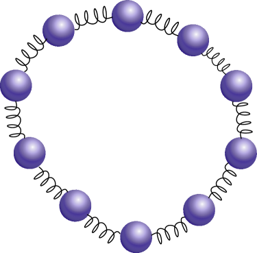
(a)

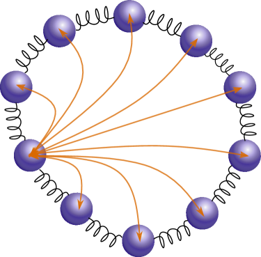
(b)

Figure 1: Cartoon representing the ring polymer of (a) a free particle, and (b) a particle in contact with a harmonic bath. The standard harmonic springs are depicted in black while the springs emerging from the system-bath coupling are depicted in orange. These two couplings correspond to the second and last term on the right hand side of Eq. 20, respectively. Note that, for the sake of clarity, we only draw the latter term for a single bead, but it is present between all pairs of beads.

In Fig. 1 we show a cartoon representation of the ring polymer corresponding to one free particle and to the same particle coupled to a harmonic bath. The second term on the right-hand side of Eq. 20, the ‘friction springs’, couple the beads beyond the nearest neighbours, representing a term that is non-local in imaginary time (see further discussion in Appendix B). For a positive-definite friction tensor, these friction spring-terms increase the effective coupling among the beads causing the system to behave more classically when compared to the free-particle system. Indeed, in the low friction limit, the zero-point energy (ZPE) of a damped harmonic oscillator with frequency $\omega$, $E^{\omega,\eta}_{\text{ZPE}}$, decreases as

$$\begin{split}E^{\omega,\eta}_{\text{ZPE}}-E^{\omega,0}_{\text{ZPE}}\approx-\frac{\hbar\tilde{\eta}_{0}\omega_{D}}{4\omega}+\frac{\hbar\tilde{\eta}(0)}{2\pi}\ln\frac{\omega_{D}}{\omega}<0,\end{split}$$ (21)

where a spectral density with Drude cutoff $J^{\text{Drude}}(\omega)=\eta\omega\omega_{D}^{2}/(\omega_{D}^{2}+\omega^{2})$ was assumed in the derivation Ingold (2002).

Next, we show that when the friction is position-independent, we can derive an extension of the Grote-Hynes approximation for the reaction rate in the deep-tunneling regime.

Extension of the Grote-Hynes approximation into the Deep Tunneling Regime

Grote, HynesGrote and Hynes (1980, 1981) and Pollak Pollak (1986) showed that for intermediate to strong friction values, the classical reaction rate of the system-bath model can be written in terms of the system rate and $\tilde{\eta}(\omega)$ as

$$\begin{split}k_{\text{TST}}(\tilde{\eta})=k^{\text{sys}}_{\text{TST}}\bigg{\{}\bigg{[}\left(\frac{\tilde{\eta}(\omega_{0})}{2m\omega^{{\ddagger}}}\right)^{2}+1\bigg{]}^{1/2}-\frac{\tilde{\eta}(\omega_{0})}{2m\omega^{{\ddagger}}}\bigg{\}},\end{split}$$ (22)

where $k^{\text{sys}}_{\text{TST}}$ and $k_{\text{TST}}$ are the transition state rates for the system and system bath, respectively, $m$ the system mass, $\omega^{{\ddagger}}$ the imaginary frequency of the system at the barrier top, and $\omega_{0}$ is given by the relation

$$\begin{split}\frac{\omega_{0}}{\omega^{{\ddagger}}}&=\bigg{[}\left(\frac{\tilde{\eta}(\omega_{0})}{2m\omega^{{\ddagger}}}\right)^{2}+1\bigg{]}^{1/2}-\frac{\tilde{\eta}(\omega_{0})}{2m\omega^{{\ddagger}}}.\end{split}$$ (23)

As elegantly proved by PollakPollak (1986), Eq. 23 can be interpreted as a renormalized effective barrier frequency due to dissipation. In a similar spirit, we would like to derive a relation between the RPI rates of the system without dissipation and the RPI-EF rates which include dissipation. Moreover, it would be desirable to obtain such a relation without resorting to any assumption on the potential energy surface. The last condition forbids any direct relation between $k_{\text{inst}}(\beta,\eta)$ and $k_{\text{inst}}(\beta,\eta=0)$ at the same temperature, since both instanton pathways will have different extensions and therefore will be affected by different regions of the potential energy surface. Another possibility to tackle this problem is to ask the following question: “Given an instanton obtained at $T_{a}$ on $U_{P}^{\text{sys}}$, at which temperature $T_{b}$ will an instanton obtained on $U_{P}^{\text{MF}}$ present (approximately) the same geometry?”. Mathematically, given $\beta_{a}=1/k_{B}T_{a}$ and $\bm{q}_{a}$ the solution to

$$\begin{split}0&=\frac{\partial S_{P}^{\text{sys}}(\beta_{a},\bm{q}_{a})}{\partial q_{i}^{(k)}},\quad k=1,\dots,P\quad i=1,\dots,3N,\end{split}$$ (24)

we aim to find $\beta_{b}$ such that $\bm{q}_{a}$ is an approximate solution to

$$\begin{split}0&=\frac{\partial S_{P}^{\text{MF}}(\beta_{b},\bm{q}_{a})}{\partial q_{i}^{(k)}},\quad k=1,\dots,P,\quad i=1,\dots,3N.\end{split}$$ (25)

In the previous equations the sub-index $a$ and $b$ refer to the inverse temperatures $\beta_{a}$ and $\beta_{b}$, respectively. Using Eq. 1 and going to the RP normal mode representation, we look for $\beta_{b}$ that simultaneously satisfies

$$\begin{split}0&=\frac{\partial S^{\text{sys}}(\beta_{a},\textbf{q}_{a})/\hbar}{\partial Q_{i}^{(l)}}=\beta^{a}_{P}\bigg{[}\frac{\partial V(\textbf{q}_{a})}{\partial Q_{i}^{(l)}}+m_{i}{\omega_{l}^{a}}^{2}Q_{i}^{(l)}\bigg{]}\\ 0&=\frac{\partial V(\textbf{q}_{a})}{\partial Q_{i}^{(l)}}+m_{i}{\omega_{l}^{a}}^{2}Q_{i}^{(l)},\end{split}$$ (26)

and

$$\begin{split}0&=\frac{\partial S^{\text{MF}}(\beta_{b},\textbf{q}_{a})/\hbar}{\partial Q_{i}^{(l)}}=\beta^{b}_{P}\bigg{[}\frac{\partial V(\textbf{q}_{b})}{\partial Q_{i}^{(l)}}+m_{i}{\omega_{l}^{b}}^{2}Q_{i}^{(l)}+\tilde{\eta}(\omega_{l})Q_{i}^{(l)}\bigg{]}\\ 0&=\frac{\partial V(\textbf{q}_{a})}{\partial Q_{i}^{(l)}}+m_{i}{\omega_{l}^{b}}^{2}Q_{i}^{(l)}+\tilde{\eta}(\omega^{b}_{l})\omega^{b}_{l}Q_{i}^{(l)},\end{split}$$ (27)

for $l=-P/2+1,\dots,P/2$ and $i=1,\dots,3N$.

We combine Eq. 26 and Eq. 27 to get

$$\begin{split}{\omega_{l}^{b}}^{2}+\frac{\tilde{\eta}({\omega_{l}^{b}})}{m_{i}}{{\omega_{l}^{b}}}-{\omega_{l}^{a}}^{2}=0,\end{split}$$ (28)

where $Q_{i}^{(l)}\neq 0$ was assumed since in that case Eq. 26 and 27 became identical and therefore the latter is trivially satisfied when the former is. In the limit of $P\to\infty$, we have $\omega_{l}=\frac{2\pi|l|}{\beta\hbar}$, so we can solve the quadratic equation for $T_{b}$ to obtain

$$\begin{split}T_{b}/T_{c}^{\circ}=\sqrt{\bigg{(}\frac{\tilde{\eta}(\omega_{l}^{b})}{2m_{i}{\omega^{\ddagger}}}\bigg{)}^{2}\frac{1}{l^{2}}+\left(\frac{T_{a}}{T_{c}^{\circ}}\right)^{2}}-\frac{\tilde{\eta}(\omega_{l}^{b})}{2m_{i}{\omega^{\ddagger}}}\frac{1}{l},\end{split}$$ (29)

where $T_{c}^{\circ}$ is given by Eq. 7 and $l\neq 0$. The previous equation cannot be fulfilled for all values of $l$ unless $\tilde{\eta}$ has a very specific frequency dependence. In part II of this paper, we will see that we can exploit the fact that the normal modes with $|l|=1$ dominate the instanton pathways, and thus we can solve Eq. 29 for $|l|=1$. Note that this equation has to be solved self-consistently, since $\omega^{b}_{l}$ depends on $T^{b}$. Interestingly, Eq. 39 results from Eq. 29 for $T_{a}=T_{c}$, so the latter equation can be interpreted as a generalization of the former. Eq. 29 allows one to compute the tunneling rates of a system coupled to a bath by only finding instanton pathways of the uncoupled system at a scaled temperature. Thus, it can be interpreted as a generalization of the GH equation into the deep tunneling regime.

III.2 Position Dependent Friction

The simplest system-bath coupling function that results in a position dependence of the friction is given by

$$\begin{split}f_{ij}(\bm{q})=c_{j}g_{i}(\bm{q}),\end{split}$$ (30)

leading to the following spectral density

$$\begin{split}J_{il}(\bm{q},\omega)=\bigg{(}\frac{\partial g_{i}(\bm{q})}{\partial q_{l}}\bigg{)}^{2}\frac{\pi}{2}\sum_{j=1}^{N_{b}}\frac{c_{j}^{2}}{\mu_{j}\omega}(\delta(\omega-\omega_{j})+\delta(\omega+\omega_{j})).\end{split}$$ (31)

This coupling function is equivalent to assuming that the zero-frequency value of the friction tensor $\tilde{\eta}(\bm{q},\omega=0)$ is position-dependent and its frequency dependence is identical for all positions Straus, Gomez Llorente, and Voth (1993). Thus, it is sometimes referred to as ‘separable coupling’, and can be shown to yield a lower limit for the tunneling rate Caldeira and Leggett (1983). The MF-RP potential in this scenario becomes

$$\begin{split}U^{\text{MF}}_{P}=&U^{\text{sys}}_{P}+\\ &\sum_{l=-P/2+1}^{P/2}\sum_{i=1}^{3N}\sum_{j=1}^{N_{b}}\frac{1}{2}\frac{c_{j}^{2}\omega_{l}^{2}}{\mu_{j}(\omega_{j}^{2}+\omega_{l}^{2})\omega_{j}^{2}}\bigg{[}\sum_{k=1}^{P}C_{lk}g(\textbf{q}^{(k)})_{i}\bigg{]}^{2}\\ =&U^{\text{sys}}_{P}+\\ &\sum_{l=-P/2+1}^{P/2}\sum_{i=1}^{3N}\sum_{j=1}^{N_{b}}\bigg{[}\frac{1}{2}\frac{c_{j}^{2}\omega_{l}^{2}}{\mu_{j}(\omega_{j}^{2}+\omega_{l}^{2})\omega_{j}^{2}}\bigg{]}\times\\ &\bigg{[}\sum_{k=1}^{P}C_{lk}\int_{0}^{1}ds\frac{dg(\textbf{q}^{\text{k}}(s))_{i}}{ds}-\sum_{k=1}^{P}C_{lk}g(\textbf{q}^{\text{ref}})_{i}\bigg{]}^{2}\\ =&U^{\text{sys}}_{P}+\\ &\sum_{l=-P/2+1}^{P/2}\sum_{i=1}^{3N}\sum_{j=1}^{N_{b}}\bigg{[}\frac{1}{2}\frac{c_{j}^{2}\omega_{l}^{2}}{\mu_{j}(\omega_{j}^{2}+\omega_{l}^{2})\omega_{j}^{2}}\bigg{]}\times\\ &\bigg{[}\sum_{k=1}^{P}C_{lk}\int_{0}^{1}ds\frac{dg(\textbf{q}^{\text{k}}(s))_{i}}{ds}\bigg{]}^{2},\\ \end{split}$$ (32)

where we consider that $\textbf{q}^{k}(s):\mathbb{R}\rightarrow{}\mathbb{R}^{3N}$ is a parametrization, such that $\textbf{q}^{k}(0)=\textbf{q}^{\text{ref}}$ and $\textbf{q}^{k}(1)=\textbf{q}^{\text{k}}$. In the last line we used that $\sum_{k=1}^{P}C_{lk}g(\textbf{q}^{\text{ref}})_{i}$ only contributes to the $l=0$ term and, since $\omega_{0}=0$, its contribution vanishes. As a consequence, the reference position is a free parameter which does not affect the results.

We continue by applying the chain rule

$$\begin{split}U^{\text{MF}}_{P}=&U^{\text{sys}}_{P}+\sum_{l=-P/2+1}^{P/2}\sum_{i=1}^{3N}\bigg{[}\sum_{k=1}^{P}C_{lk}\int_{0}^{1}ds\sum_{r}\frac{\partial q^{\text{k}}_{r}(s)}{\partial s}\times\\ &\bigg{(}\sum_{j=1}^{N_{b}}\frac{1}{2}\frac{c_{j}^{2}}{\mu_{j}\omega_{j}^{2}}\frac{\partial g(\textbf{q}^{\text{k}}(s))_{i}}{\partial q^{\text{k}}_{r}}^{2}\frac{\omega_{l}^{2}}{(\omega_{j}^{2}+\omega_{l}^{2})}\bigg{)}^{1/2}\bigg{]}^{2},\end{split}$$ (33)

and finally, by rearranging the terms, we obtain

$$\begin{split}U^{\text{MF}}_{P}=&U^{\text{sys}}_{P}+\\ &\sum_{l=-P/2+1}^{P/2}\sum_{i=1}^{3N}\frac{\omega_{l}}{2}\bigg{[}\sum_{k=1}^{P}C_{lk}\bigg{(}\sum_{r=1}^{3N}\int_{\bm{q}^{\text{ref}}}^{\bm{q}^{(k)}}\tilde{\eta}_{ir}(\bm{q}^{\prime},\omega_{k})^{1/2}\cdot d\bm{q_{r}}^{\prime}\bigg{)}\bigg{]}^{2}\\ &=U^{\text{sys}}_{P}+\\ &\sum_{l=-P/2+1}^{P/2}\sum_{i=1}^{3N}\frac{\omega_{l}}{2}\bigg{[}\sum_{k=1}^{P}C_{lk}\bigg{(}\int_{\bm{q}^{\text{ref}}}^{\bm{q}^{(k)}}\tilde{\bm{\eta}_{i}}(\bm{q}^{\prime},\omega_{k})^{1/2}\cdot d\bm{q}^{\prime}\bigg{)}\bigg{]}^{2},\end{split}$$ (34)

with $\tilde{\bm{\eta}}_{i}$ being the $i$-th row of the friction tensor. We note that a straightforward extension of the Grote-Hynes approximation is not possible in this case. For completeness, for a one-dimensional system, the previous equation simplifies to

$$\begin{split}U^{\text{MF}}_{P}=&U^{\text{sys}}_{P}+\sum_{l=-P/2+1}^{P/2}\frac{\omega_{l}}{2}\bigg{[}\sum_{k=1}^{P}C_{lk}\int_{q^{\text{ref}}}^{q^{(k)}}dq^{\prime}\tilde{\eta}(q^{\prime},\omega_{l})^{1/2}\bigg{]}^{2}.\end{split}$$ (35)

III.3 Renormalization of cross-over temperature

Naturally, the coupling of the bath to the system impacts the nuclear tunneling. One can study, for example, how the tunneling cross-over temperature is modified by the coupling to the bath. A trivial stationary point on the extended phase space of the ring polymer in the pathway that connects reactants and products can be found by locating all the beads at the top of the barrier. For a 1D system with position-dependent or independent friction under the parabolic barrier approximation, one can write

$$\begin{split}\lambda_{l}&=\sqrt{\omega_{l}^{2}+\frac{\tilde{\eta}(\omega_{l})}{m}\omega_{l}-(\omega^{\ddagger})^{2},}\end{split}$$ (36)

where $\omega_{l}=2\omega_{P}\sin(|l|\pi/P)$ are the free RP normal mode frequencies, $i\omega^{{\ddagger}}$ is the imaginary frequency at the barrier top, and $\tilde{\eta}$ has been evaluated at the barrier top. In the limit of large $P$, $\omega_{l}=2\pi|l|/\beta\hbar$ and the lowest three frequencies are

$$\begin{split}\lambda_{0}&=i\omega^{{\ddagger}}\\ \lambda_{\pm 1}&=\sqrt{\frac{4\pi^{2}}{\beta^{2}\hbar^{2}}+\frac{2\pi\tilde{\eta}(\omega_{1})}{\beta\hbar m}-(\omega^{\ddagger})^{2}},\end{split}$$ (37)

where $\omega_{1}$ refers to the first Matsubara frequency Matsubara (1955), which depends on the temperature. The cross-over temperature is the temperature, $\beta^{\text{sb}}_{c}=1/k_{B}T_{c}^{\text{sb}}$, below which $\lambda_{\pm 1}$ becomes imaginary (i.e. $\lambda_{\pm 1}^{2}$ becomes negative) and the location of the first-order saddle point is not at the top of the barrier, i.e. a non-trivial instanton pathway becomes possible. By taking $\lambda_{\pm 1}=0$ in the previous equation and solving the quadratic equation for $\beta^{\text{sb}}_{c}$, one obtains

$$\begin{split}k_{B}T^{\text{sb}}_{c}&=\frac{1}{\beta^{\text{sb}}_{c}}=\frac{\hbar}{4\pi}\left(\sqrt{\frac{\tilde{\eta}(\omega_{1})^{2}}{m^{2}}+4\omega^{{\ddagger}2}}-\sqrt{\frac{\tilde{\eta}(\omega_{1})^{2}}{m^{2}}}\right),\end{split}$$ (38)

where $\omega_{1}$ is evaluated at $T_{c}^{\text{sb}}$. Finally, identifying $T_{c}^{\circ}$ (Eq. 7) in the equation above leads to

$$\begin{split}T_{c}^{\text{sb}}=T^{\circ}_{c}\times\bigg{[}\sqrt{\bigg{(}\frac{\tilde{\eta}(\omega_{1})}{2m\omega^{\ddagger}}\bigg{)}^{2}+1}-\frac{\tilde{\eta}(\omega_{1})}{2m\omega^{\ddagger}}\bigg{]}.\end{split}$$ (39)

Since $\omega_{1}$ depends on $T_{c}^{\text{sb}}$, Eq. 39 has to be solved self-consistently. The number between square brackets is always positive and less than 1, so $T_{c}^{\text{sb}}$ is always lower than $T_{c}^{\circ}$. Moreover, it is straightforward to see that the stronger the friction, the lower $T_{c}^{\text{sb}}$ becomes, and tunneling becomes less important at a given temperature. If the friction tensor is position-dependent, $T_{c}^{\text{sb}}$ can be calculated by Eq. 39 replacing $\tilde{\eta}(\omega_{1})$ by $\tilde{\eta}(\bm{q}^{\ddagger},\omega_{1})$ where $\bm{q}^{\ddagger}$ refers to the transition state geometry.

IV Ab initio Electronic Friction

For systems in which the ground electronic state can be approximated by effectively independent quasi-particles such as the ones obtained with Kohn-Sham (KS) density-functional theory (DFT), the adiabatic electronic friction tensor can be obtained from first-principles simulations assuming non-interacting electrons and, as shown in Appendix C, adopts the following form for t>0

$$\begin{split}\eta^{\text{el}}_{ij}(\textbf{q},t)=&\hbar\sum_{\nu,\nu^{\prime}}\braket{\psi_{\nu}}{\partial_{i}\psi_{\nu^{\prime}}}\braket{\psi_{\nu^{\prime}}}{\partial_{j}\psi_{\nu}}\Omega_{\nu\nu^{\prime}}\\ &\times(f(\epsilon_{\nu})-f(\epsilon_{\nu^{\prime}}))\cos{(\Omega_{\nu\nu^{\prime}}t)},\end{split}$$ (40)

where $f(\epsilon)$ is the state occupation given by the Fermi-Dirac occupation function, $\Omega_{\nu\nu^{\prime}}=(\epsilon_{\nu^{\prime}}-\epsilon_{\nu})/\hbar$, $\psi_{\nu}$ and $\epsilon_{\nu}$ are the KS electronic orbitals and orbital energies of the $\nu$-th level, $i$ and $j$ label the nuclear degrees of freedom, and $\partial_{i}=\partial/\partial q_{i}$. A Fourier transform of the expression above leads to the usual expression employed in Refs. Head-Gordon and Tully (1995); Dou, Miao, and Subotnik (2017); Maurer et al. (2016) and reads

$$\begin{split}\hat{\eta}^{\text{el}}_{ij}(\textbf{q},\omega)=&\pi\hbar\sum_{\nu,\nu^{\prime}}\braket{\psi_{\nu}}{\partial_{i}\psi_{\nu^{\prime}}}\braket{\psi_{\nu^{\prime}}}{\partial_{j}\psi_{\nu}}\times(f(\epsilon_{\nu})-f(\epsilon_{\nu^{\prime}}))\\ &\times\Omega_{\nu\nu^{\prime}}\delta(\Omega_{\nu{\nu^{\prime}}}-\omega),\end{split}$$ (41)

where the k-point dependence has been omitted.

Most of the applications of the MDEF approach only consider an electronic friction tensor that is local in time to avoid the complexities of handling a non-instantaneous memory kernel and normally invoke the Markov approximation. This limit is also often referred to in the literature as the quasi-static limit since the Markov approximation is normally realized by taking $\omega\to 0$ limit in Eq. 41.Hellsing and Persson (1984) In the cases where the system presents a constant density of states (DOS) around the Fermi level, an equivalent derivation is possible by applying the constant coupling approximation Head-Gordon and Tully (1995). The quasi-static limit involves the evaluation of the friction tensor in Eq. 41 for excitations infinitesimally close to the Fermi level. In practical calculations with finite k-point grids, it is numerically challenging to accurately describe the DOS at the Fermi energy. This is typically circumvented by introducing a finite width for the delta function in Eq. 41. The choice of width depends on the system and, in literature, values between 0.01 and 0.60 eV can be found.Maurer et al. (2016); Novko et al. (2019); Connor L. Box (2021); Shipley et al. (2020).

The connection of the ab initio electronic friction and the RPI rate theory might seem a trivial substitution of Eq.  41 into Eq. 34. However, as we shall show in the next section, this is not the case and in order to obtain a better connection between the electronic friction and the system-bath model used in the formulation of RPI-EF, a different expression should be employed.

IV.1 Electronic spectral density of non-interacting electrons

Starting from Eq. 40, and in a similar spirit to Eq. 10, we perform a Laplace transform to get

$$\begin{split}\tilde{\eta}_{ij}^{\text{el}}(\textbf{q},\lambda)&=\int_{0}^{\infty}dte^{-\lambda t}\eta_{ij}^{\text{el}}(\textbf{q},t)\\ &=\hbar\sum_{\nu,\nu^{\prime}}\braket{\psi_{\nu}}{\partial_{i}\psi_{\nu^{\prime}}}\braket{\psi_{\nu^{\prime}}}{\partial_{j}\psi_{\nu}}(f(\epsilon_{\nu})-f(\epsilon_{\nu^{\prime}}))\Omega_{\nu\nu^{\prime}}\\ &\times\frac{\lambda}{\lambda^{2}+\Omega_{\nu\nu^{\prime}}^{2}}.\end{split}$$ (42)

The equation above adopts the same limit for $\lambda\to 0$ as Eq. 41. However, for $\lambda>0$, instead of the $\delta$ function, we obtain a sum of Lorentzian functions of width $2\lambda$. Comparing Eq. 42 and 11, we can identify the equivalent of the spectral density in RPI-EF as

$$\begin{split}J_{ij}(\bm{q},\omega)=\pi\hbar\sum_{\nu,\nu^{\prime}}\braket{\psi_{\nu}}{\partial_{i}\psi_{\nu^{\prime}}}\braket{\psi_{\nu^{\prime}}}{\partial_{j}\psi_{\nu}}\omega^{2}\\ \times(f(\epsilon_{\nu})-f(\epsilon_{\nu^{\prime}}))\delta(\omega-\Omega_{\nu\nu^{\prime}}),\end{split}$$ (43)

which provides a seamless connection between RPI-EF and electronic friction.

In RPI-EF, the spectral density of electronic friction shown in Eq. 43 is evaluated simultaneously at the ring polymer normal mode frequencies. Thus, we have derived viable expressions to combine RPI-EF with an electronic friction formulation that can be calculated from first-principles, without any further approximations, except for the assumption of separable coupling, which we shall examine for real systems in part II of this paper. We expect that the connection of these two theories will be suitable as long as the approximations of both underlying theories remain valid.

V Conclusions

We have presented an extension of the ring-polymer instanton rate theory to describe a system coupled to a bath of harmonic oscillators through the definition of an effective friction tensor that enters the instanton ring-polymer potential energy expression. We therefore refer to this method as the RPI-EF approach. The theory is rather general and allows the inclusion of frequency and position dependence in the system-bath coupling for the calculation of thermal tunneling rates within the instanton approximation. For the case of linear coupling, we derived an approximation that allows one to predict RPI-EF reactions rates using only RPI calculations. The approximation can be understood as an extension of the Grote-Hynes approximation to the deep tunneling regime. This may be useful to estimate whether it is necessary to carry out full RPI-EF calculations for a particular reaction.

RPI-EF is a method tailored for the description of tunneling rates and based on imaginary-time trajectories. Therefore, it cannot be applied for the simulation of vibrational relaxation or scattering experiments Bünermann et al. (2015); Wodtke (2016); Jiang et al. (2021), where some kinds of NQEs and NAEs could interplay strongly. It would be interesting to write similar extensions to approaches based on path integral molecular dynamics Craig and Manolopoulos (2004); Cao and Voth (1994); Rossi, Ceriotti, and Manolopoulos (2014); Trenins, Willatt, and Althorpe (2019), since they would yield efficient approximations to model these situations. Other future directions could cover the inclusion of non-equilibirum effects through the use of non-positive definite friction tensors Bode et al. (2012); Lü et al. (2019). We hope that the derivations presented in this work stimulate further theoretical developments in this area and allow new phenomena to be explained in situations that we have not yet explored.

Appendix

V.1 Free Ring Polymer Normal Modes

The free ring polymer potential is given by setting $V=0$ in Eq. 2. The resulting potential is harmonic, however, due to the presence of degenerate eigenvalues there is no unique transformation to diagonalize it. Assuming $P$ is even, one possibility is the following orthogonal coordinate transformationCraig (2006); Markland and Manolopoulos (2008)

$$Q^{(l)}_{i}=\sum^{P}_{k=1}C_{lk}^{(P)}{q}^{k}_{i}{\quad i=1,\dots,3N,\quad l=-P/2+1,\dots,P/2},$$ (44)

where the $P\times P$ matrix $C^{(P)}$ is defined as

$$C_{lk}^{(P)}=\begin{cases}\sqrt{\frac{1}{P}}&l=0\\ \sqrt{\frac{2}{P}}\cos(\frac{2\pi kl}{n})&1\leq l\leq P/2-1\\ \sqrt{\frac{1}{P}}(-1)^{j}&l=P/2\\ \sqrt{\frac{2}{P}}\sin(\frac{2\pi kl}{P})&-P/2+1\leq l\leq-1.\\ \end{cases}$$

V.2 Mean-Field Ring Polymer Potential in Cartesian Representation for Spatially Independent Coupling

The mean-field RP potential in Cartesian representation for the linear coupling case is obtained by introducing Eq. 44 into 20 leading to

$$\begin{split}U^{\text{MF}}_{P}=&\sum_{l=1}^{P}V(q_{1}^{(l)},\dots,q_{3N}^{(l)})+\\ &\sum_{\begin{subarray}{c}k=1\\ k^{\prime}=1\end{subarray}}^{P}\sum_{i=1}^{3N}\frac{1}{2}q_{i}^{(k^{\prime})}O_{i,k,k^{\prime}}q_{i}^{(k)}+\frac{1}{2}q_{i}^{(k^{\prime})}D_{i,k,k^{\prime}}q_{i}^{(k)}\end{split}$$ (45)

with

$$\begin{split}O_{k,k^{\prime}}=m_{i}\omega_{P}^{2}(2\delta_{k,k^{\prime}}-\delta_{k,k^{\prime}-1}-\delta_{k,k^{\prime}+1})\end{split}$$ (46)

and

$$\begin{split}D_{k,k^{\prime}}=&\eta_{0}\omega_{P}\bigg{[}\sum_{l=1}^{(P-1)/2}\frac{4}{P}\sin(\pi l/P)\cos(2\pi l(k-k^{\prime})/P)\\ &-\frac{2}{P}(-1)^{k+k^{\prime}}\bigg{]},\end{split}$$ (47)

where a linear (Ohmic) spectral density was considered. In Fig. 2 we show a graphical representation of the spring coupling matrices $O_{k,k^{\prime}}$ and $D_{k,k^{\prime}}$. The latter has small but non-zero matrix elements outside the tridiagonal entries present in the former, representing coupling beyond nearest-neighbor beads. Moreover, the matrix elements decay rapidly with the increase of the bead index distances when periodic boundary conditions are considered.

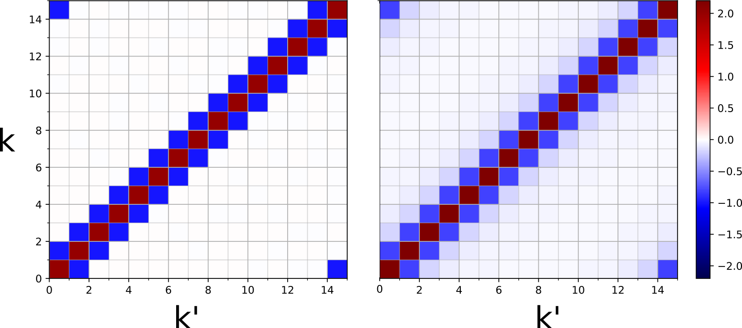
Figure 2: Spring coupling matrices $O_{k,k^{\prime}}$ (left) and $D_{k,k^{\prime}}$ (right) at 25 K for 15 beads and $\eta_{0}/m\omega_{0}=1.0$. The values have been scaled by $m\omega_{P}$ to ease visual comparison.

V.3 Arriving at Eq. 40

The steps presented in this Appendix closely follow Ref. Dou, Miao, and Subotnik (2017), and we repeat them here merely for completeness. We consider a quadratic electronic Hamiltonian of the form,

$$\begin{split}\hat{h}=\sum_{pq}h_{qp}(\mathbf{q})\hat{d}_{p}^{+}\hat{d}_{q}\end{split}$$ (48)

where $h_{qp}(\textbf{q})$ is general notation to represent that matrix elements might depend on the nuclear degrees of freedom, q, and $\hat{d}_{p}^{+}$ and $\hat{d}_{q}$ are the electronic creation and annihilation operators, respectively.

Starting from the quantum-classical Liouville equation, the electronic friction tensor in the adiabatic limit with nuclei fixed at position q can be written as Dou, Miao, and Subotnik (2017)

$$\begin{split}\eta^{\text{el}}_{ij}(\textbf{q},t)=-\text{tr}_{e}\bigg{(}\partial_{i}\hat{h}e^{-i\hat{\hat{\mathcal{L}}}t}\partial_{j}\hat{\rho}_{ss}\bigg{)}\end{split}$$ (49)

where $\hat{\hat{\mathcal{L}}}$ is the Liouvillian superoperator, $\text{tr}_{e}$ implies tracing over the electronic degrees of freedom, $\hat{\rho}_{ss}$ is the steady state electronic density matrix, and $i$ and $j$ represent two nuclear degrees of freedom.

By recalling that $e^{-i\hat{\hat{\mathcal{L}t}}}(\cdot)=e^{-i\hat{h}t/\hbar}(\cdot)e^{i\hat{h}t/\hbar}$, the invariance of the trace under cyclic permutations, and considering the quadratic Hamiltonian presented above we find

$$\begin{split}\eta^{\text{el}}_{ij}(\textbf{q},t)&=-\text{tr}_{e}\bigg{(}e^{i\hat{h}t}\partial_{i}\hat{h}e^{-i\hat{h}t}\partial_{j}\hat{\rho}_{ss}\bigg{)}\\ &=-\sum_{mn}\partial_{i}h_{nm}\text{tr}_{e}\bigg{(}e^{i\hat{h}t}\hat{d}_{m}^{+}\hat{d}_{n}e^{-i\hat{h}t}\partial_{j}\hat{\rho}_{ss}\bigg{)}\\ &=-\sum_{mn}\partial_{i}h_{nm}\text{tr}_{e}\bigg{(}e^{i\hat{h}t}\hat{d}_{m}^{+}e^{-i\hat{h}t}e^{i\hat{h}t}\hat{d}_{n}e^{-i\hat{h}t}\partial_{j}\hat{\rho}_{ss}\bigg{)}.\\ \end{split}$$ (50)

By noting that $e^{i\hat{h}t/\hbar}\hat{d}_{m}^{+}e^{-i\hat{h}t/\hbar}=\sum_{a}(e^{i\hat{h}t/\hbar})_{ma}\hat{d}_{a}^{+}$, and $e^{i\hat{h}t/\hbar}\hat{d}_{n}e^{-i\hat{h}t/\hbar}=\sum_{b}(e^{-i\hat{h}t/\hbar})_{bn}\hat{d}_{b}$ (see Supporting Information in Ref. Dou, Miao, and Subotnik (2017)), and defining $\sigma_{ab}^{ss}=\text{tr}_{e}(\hat{d}_{a}^{+}\hat{d}_{b}\hat{\rho}_{ss})$, Eq. LABEL:eq:eta2 can be expressed as

$$\begin{split}\eta^{\text{el}}_{ij}(\textbf{q},t)&=-\sum_{mnab}\partial_{i}h_{nm}(e^{i\hat{h}t/\hbar})_{ma}(e^{-i\hat{h}t/\hbar})_{bn}\text{tr}_{e}\bigg{(}\hat{d}_{a}^{+}\hat{d}_{b}\partial_{j}\hat{\rho}_{ss}\bigg{)}\\ &=-\sum_{mnab}\partial_{i}h_{nm}(e^{i\hat{h}t/\hbar})_{ma}\partial_{j}\sigma_{ab}^{ss}(e^{-i\hat{h}t/\hbar})_{bn}\\ &=-\sum_{n}\bigg{(}\partial_{i}\hat{h}e^{i\hat{h}t/\hbar}\partial_{j}\sigma^{ss}e^{-i\hat{h}t/\hbar}\bigg{)}_{nn}\end{split}$$ (51)

where $\sum_{n}$ represents a sum over electronic orbitals. If we take the basis in which $\hat{h}$ is diagonal,

$$\begin{split}\hat{h}=\sum_{\nu}\epsilon_{\nu}\Ket{\psi_{\nu}}\Bra{\psi_{\nu}},\end{split}$$ (52)

Eq. 51 simplifies to

$$\begin{split}\eta^{\text{el}}_{ij}(\textbf{q},t)&=-\sum_{\nu,\nu^{\prime}}\Bra{\psi_{\nu}}\partial_{i}\hat{h}\Ket{\psi_{\nu^{\prime}}}e^{i\epsilon_{\nu^{\prime}}t/\hbar}\Bra{\psi_{\nu^{\prime}}}\partial_{j}\sigma^{ss}\Ket{\psi_{\nu}}e^{-i\epsilon_{\nu}t/\hbar}.\end{split}$$ (53)

At equilibrium, we can write $\hat{\sigma}^{ss}$ as

$$\begin{split}\hat{\sigma}^{ss}=\sum_{\nu}f(\epsilon_{\nu})\Ket{\psi_{\nu}}\Bra{\psi_{\nu}},\end{split}$$ (54)

and therefore, the second matrix element in Eq. 53 can be evaluated as

$$\begin{split}\Bra{\psi_{\nu^{\prime}}}\partial_{i}\hat{\sigma}^{ss}\Ket{\psi_{\nu}}=&\partial_{i}\epsilon_{\nu}\frac{f(\epsilon_{k})}{\partial\epsilon_{\nu}}\delta_{\nu\nu^{\prime}}\\ &+(f(\epsilon_{\nu})-f(\epsilon_{\nu^{\prime}}))\braket{\psi_{\nu^{\prime}}}{\partial_{i}\psi_{\nu}}.\end{split}$$ (55)

Introducing Eq. 55 into Eq. 53, and using

$$\begin{split}\partial_{i}\Bra{\psi_{\nu}}\hat{h}\Ket{\psi_{\nu^{\prime}}}&=\partial_{i}\epsilon_{\nu}\delta_{\nu\nu^{\prime}}\\ &=\Bra{\psi_{\nu}}\partial_{i}\hat{h}\Ket{\psi_{\nu^{\prime}}}+\braket{\psi_{\nu}}{\partial_{i}\psi_{\nu^{\prime}}}(\epsilon_{\nu}-\epsilon_{\nu}^{\prime}),\end{split}$$ (56)

leads to

$$\begin{split}\eta^{\text{el}}_{ij}(\textbf{q},t)=&\sum_{\nu,\nu^{\prime}}\Bigg{[}\braket{\psi_{\nu}}{\partial_{i}\psi_{\nu^{\prime}}}(\epsilon_{\nu}^{\prime}-\epsilon_{\nu})+\partial_{i}\epsilon_{\nu}\delta_{\nu\nu^{\prime}}\Bigg{]}\\ &\times\Bigg{[}\partial_{j}\epsilon_{\nu}\frac{f(\epsilon_{\nu})}{\partial\epsilon_{\nu}}\delta_{\nu\nu^{\prime}}+(f(\epsilon_{\nu})-f(\epsilon_{\nu}^{\prime}))\braket{\psi_{\nu^{\prime}}}{\partial_{j}\psi_{\nu}}\Bigg{]}\\ &\times e^{-i(\epsilon_{\nu}-\epsilon_{\nu^{\prime}})t/\hbar}.\end{split}$$ (57)

Finally, upon noticing that the factors in front of the exponential are invariant under the exchange of orbital labels such that the imaginary part of the complex exponential vanishes, and the fact that for $\nu=\nu^{\prime}$ the expression is zero, one arrives to Eq. 40 presented in the main text. This expression agrees with an alternative recent derivation based on the exact factorization of the electronic-nuclear wavefunction Martinazzo and Burghardt (2021).

References

- Bartels et al. (2011) C. Bartels, R. Cooper, D. J. Auerbach, and A. M. Wodtke, Chem. Sci. 2, 1647 (2011).
- Wodtke (2016) A. M. Wodtke, Chem. Soc. Rev. 45, 3641 (2016).
- Auerbach, Tully, and Wodtke (2021) D. J. Auerbach, J. C. Tully, and A. M. Wodtke, Nat. Sciences 1 (2021).
- Schindler, Diesing, and Hasselbrink (2011) B. Schindler, D. Diesing, and E. Hasselbrink, J. Chem. Phys. 134, 034705 (2011).
- Cohen et al. (2005) O. Cohen, G. Bartal, H. Buljan, T. Carmon, J. W. Fleischer, M. Segev, and D. N. Christodoulides, Nature 433, 503 (2005).
- Box et al. (2021) C. L. Box, Y. Zhang, R. Yin, B. Jiang, and R. J. Maurer, J. Am. Chem. Soc. Au 1, 164 (2021).
- Persson and Hellsing (1982) M. Persson and B. Hellsing, Phys. Rev. Lett. 49, 662 (1982).
- Tully, Gomez, and Head-Gordon (1993) J. C. Tully, M. Gomez, and M. Head-Gordon, J. Vac. Sci. Technol. A 11, 1914 (1993).
- Rittmeyer et al. (2015) S. P. Rittmeyer, J. Meyer, J. I. n. Juaristi, and K. Reuter, Phys. Rev. Lett. 115, 046102 (2015).
- Dou and Subotnik (2016) W. Dou and J. E. Subotnik, J. Chem. Phys. 144, 024116 (2016).
- Shenvi, Roy, and Tully (2009) N. Shenvi, S. Roy, and J. C. Tully, J. Chem. Phys. 130, 174107 (2009).
- Ryabinkin and Izmaylov (2017) I. G. Ryabinkin and A. F. Izmaylov, J. Phys. Chem. Lett. 8, 440 (2017), 1611.06525 .
- Head-Gordon and Tully (1995) M. Head-Gordon and J. C. Tully, J. Chem. Phys. 103, 10137 (1995).
- Maurer et al. (2016) R. J. Maurer, M. Askerka, V. S. Batista, and J. C. Tully, Phys. Rev. B 94, 115432 (2016).
- Blanco-Rey et al. (2014) M. Blanco-Rey, J. I. Juaristi, R. Díez Muiño, H. F. Busnengo, G. J. Kroes, and M. Alducin, Phys. Rev. Lett. 112, 103203 (2014).
- Dou and Subotnik (2018) W. Dou and J. E. Subotnik, J. Chem. Phys. 148, 230901 (2018).
- Coffman and Subotnik (2018) A. J. Coffman and J. E. Subotnik, Phys. Chem. Chem. Phys. 20, 9847 (2018).
- Zhang et al. (2019) Y. Zhang, R. J. Maurer, H. Guo, and B. Jiang, Chem. Sci. 10, 1089 (2019).
- Spiering et al. (2019) P. Spiering, K. Shakouri, J. Behler, G.-J. Kroes, and J. Meyer, J. Phys. Chem. Lett. 10, 2957 (2019).
- Kandratsenka et al. (2018) A. Kandratsenka, H. Jiang, Y. Dorenkamp, S. M. Janke, M. Kammler, A. M. Wodtke, and O. Bünermann, Proc. Natl. Acad. Sci. USA 115, 680 (2018).
- Bünermann et al. (2015) O. Bünermann, H. Jiang, Y. Dorenkamp, A. Kandratsenka, S. M. Janke, D. J. Auerbach, and A. M. Wodtke, Science 350, 1346 (2015).
- Forsythe and Makri (1998) K. M. Forsythe and N. Makri, J. Chem. Phys. 108, 6819 (1998).
- Kimizuka, Ogata, and Shiga (2019) H. Kimizuka, S. Ogata, and M. Shiga, Phys. Rev. B 100, 024104 (2019).
- Rossi, Ceriotti, and Manolopoulos (2016) M. Rossi, M. Ceriotti, and D. E. Manolopoulos, J. Phys. Chem. Lett. 7, 3001 (2016).
- Kimizuka and Shiga (2021) H. Kimizuka and M. Shiga, Phys. Rev. Mater. 5, 065406 (2021).
- Fang et al. (2017) W. Fang, J. O. Richardson, J. Chen, X.-Z. Li, and A. Michaelides, Phys. Rev. Lett. 119, 126001 (2017).
- Kimizuka, Ogata, and Shiga (2018) H. Kimizuka, S. Ogata, and M. Shiga, Phys. Rev. B 97, 014102 (2018).
- Richardson (2018) J. O. Richardson, Int. Rev. Phys. Chem. 37, 171 (2018).
- Hellsing and Persson (1984) B. Hellsing and M. Persson, Phys. Scr. 29, 360 (1984).
- Richardson and Althorpe (2009) J. O. Richardson and S. C. Althorpe, J. Chem. Phys. 131, 214106 (2009).
- Arnaldsson (2007) A. Arnaldsson, Calculation of quantum mechanical rate constants directly from ab initio atomic forces, Ph.D. thesis, University of Washington (2007).
- Miller (1975) W. H. Miller, J. Chem. Phys. 62, 1899 (1975).
- Grifoni, Piccini, and Parrinello (2019) E. Grifoni, G. Piccini, and M. Parrinello, Proc. Natl. Acad. Sci. USA 116, 4054 (2019).
- Richardson (2016) J. O. Richardson, J. Chem. Phys. 144, 114106 (2016).
- Althorpe (2011) S. C. Althorpe, J. Chem. Phys. 134, 114104 (2011).
- Affleck (1981) I. Affleck, Phys. Rev. Lett. 46, 388 (1981).
- Rommel, Goumans, and Kästner (2011) J. B. Rommel, T. P. M. Goumans, and J. Kästner, J. Chem. Theor. Comp. 7, 690 (2011).
- Rommel et al. (2012) J. B. Rommel, Y. Liu, H.-J. Werner, and J. Kästner, J. Phys. Chem. B 116, 13682 (2012).
- Litman et al. (2019) Y. Litman, J. O. Richardson, T. Kumagai, and M. Rossi, J. Am. Chem. Soc 141, 2526 (2019).
- Litman and Rossi (2020) Y. Litman and M. Rossi, Phys. Rev. Lett. 125, 216001 (2020).
- Gillan (1987) M. J. Gillan, J. Phys. C: Solid State Phys. 20, 3621 (1987).
- Weiss (2008) U. Weiss, Quantum Dissipative Systems, 3rd ed. (WORLD SCIENTIFIC, 2008).
- Caldeira and Leggett (1983) A. Caldeira and A. Leggett, Ann. Phys. 149, 374 (1983).
- Feynman and Hibbs (1965) R. P. Feynman and A. R. Hibbs, Quantum mechanics and path integrals, International series in pure and applied physics (McGraw-Hill, New York, NY, 1965).
- Markland and Manolopoulos (2008) T. E. Markland and D. E. Manolopoulos, J. Chem. Phys 129, 024105 (2008).
- Kleinert (2009) H. Kleinert, Path Integrals in Quantum Mechanics, Statistics, Polymer Physics, and Financial Markets, 5th ed. (WORLD SCIENTIFIC, 2009).
- Ranya and Ananth (2020) S. Ranya and N. Ananth, J. Chem. Phys. 152, 114112 (2020).
- Lawrence et al. (2019) J. E. Lawrence, T. Fletcher, L. P. Lindoy, and D. E. Manolopoulos, J. Chem. Phys. 151, 114119 (2019).
- Lawrence and Manolopoulos (2020) J. E. Lawrence and D. E. Manolopoulos, J. Chem. Phys. 152, 204117 (2020).
- Hertl et al. (2021) N. Hertl, R. Martin-Barrios, O. Galparsoro, P. Larrégaray, D. J. Auerbach, D. Schwarzer, A. M. Wodtke, and A. Kandratsenka, J. Phys. Chem. C 125, 14468 (2021).
- Kubo (1966) R. Kubo, Rep. Prog. Phys 29, 255 (1966).
- Ingold (2002) G.-L. Ingold, “Path integrals and their application to dissipative quantum systems,” in Coherent Evolution in Noisy Environments, edited by A. Buchleitner and K. Hornberger (Springer Berlin Heidelberg, Berlin, Heidelberg, 2002) pp. 1–53.
- Grote and Hynes (1980) R. F. Grote and J. T. Hynes, J. Chem. Phys. 73, 2715 (1980).
- Grote and Hynes (1981) R. F. Grote and J. T. Hynes, J. Chem. Phys. 74, 4465 (1981).
- Pollak (1986) E. Pollak, J. Chem. Phys. 85, 865 (1986).
- Straus, Gomez Llorente, and Voth (1993) J. B. Straus, J. M. Gomez Llorente, and G. A. Voth, J. Chem. Phys. 98, 4082 (1993).
- Matsubara (1955) T. Matsubara, Progress of Theoretical Physics 14, 351 (1955).
- Dou, Miao, and Subotnik (2017) W. Dou, G. Miao, and J. E. Subotnik, Phys. Rev. Lett. 119, 046001 (2017).
- Novko et al. (2019) D. Novko, J. C. Tremblay, M. Alducin, and J. I. Juaristi, Phys. Rev. Lett. 122, 016806 (2019).
- Connor L. Box (2021) R. J. M. Connor L. Box, Wojciech G. Stark, (2021), arXiv:2112.00121 .
- Shipley et al. (2020) A. M. Shipley, M. J. Hutcheon, M. S. Johnson, R. J. Needs, and C. J. Pickard, Phys. Rev. B 101, 224511 (2020).
- Jiang et al. (2021) H. Jiang, X. Tao, M. Kammler, F. Ding, A. M. Wodtke, A. Kandratsenka, T. F. Miller, and O. Bünermann, J. Phys. Chem. Lett. 12, 1991 (2021).
- Craig and Manolopoulos (2004) I. R. Craig and D. E. Manolopoulos, J. Chem. Phys. 121, 3368 (2004).
- Cao and Voth (1994) J. Cao and G. A. Voth, J. Chem. Phys. 100, 5106 (1994).
- Rossi, Ceriotti, and Manolopoulos (2014) M. Rossi, M. Ceriotti, and D. E. Manolopoulos, J. Chem. Phys. 140, 234116 (2014).
- Trenins, Willatt, and Althorpe (2019) G. Trenins, M. J. Willatt, and S. C. Althorpe, J. Chem. Phys. 151, 054109 (2019).
- Bode et al. (2012) N. Bode, S. V. Kusminskiy, R. Egger, and F. v. Oppen, Beilstein Journal of Nanotechnology 3, 144 (2012), 1109.6043 .
- Lü et al. (2019) J.-T. Lü, B.-Z. Hu, P. Hedegård, and M. Brandbyge, Prog. Surf. Sci. 94, 21 (2019).
- Craig (2006) I. R. Craig, Ring polymer molecular dynamics, Ph.D. thesis, University of Oxford (2006).
- Martinazzo and Burghardt (2021) R. Martinazzo and I. Burghardt, (2021), arXiv:2108.02622 .