The Gaia-ESO Survey: The analysis of the hot-star spectra
Abstract
Context. The Gaia-ESO Survey (GES) is a large public spectroscopic survey that has collected, over a period of six years, spectra of stars. This survey provides not only the reduced spectra, but also the stellar parameters and abundances resulting from the analysis of the spectra.
Aims. The GES dataflow is organised in 19 working groups. Working group 13 (WG13) is responsible for the spectral analysis of the hottest stars (O, B, and A type, with a formal cutoff of K) that were observed as part of GES. We present the procedures and techniques that have been applied to the reduced spectra in order to determine the stellar parameters and abundances of these stars.
Methods. The procedure used was similar to that of other working groups in GES. A number of groups (called Nodes) each independently analyse the spectra via state-of-the-art techniques and codes. Specific for the analysis in WG13 was the large temperature range covered ( K), requiring the use of different analysis codes. Most Nodes could therefore only handle part of the data. Quality checks were applied to the results of these Nodes by comparing them to benchmark stars, and by comparing them to one another. For each star the Node values were then homogenised into a single result: the recommended parameters and abundances.
Results. Eight Nodes each analysed part of the data. In total 17 693 spectra of 6462 stars were analysed, most of them in 37 open star clusters. The homogenisation led to stellar parameters for 5584 stars. Abundances were determined for a more limited number of stars. The elements studied are He, C, N, O, Ne, Mg, Al, Si, and Sc. Abundances for at least one of these elements were determined for 292 stars.
Conclusions. The hot-star data analysed here, as well as the GES data in general, will be of considerable use in future studies of stellar evolution and open clusters.
Key Words.:
Surveys – Catalogs – Stars: fundamental parameters – Stars: abundances – Stars: early-type – Techniques: spectroscopic1 Introduction
The Gaia-ESO Survey111http://www.gaia-eso.eu (GES; Gilmore et al. 2012, 2022; Randich et al. 2013, 2022) is a large public spectroscopic survey that observed stars in the field and in clusters of the Milky Way. The observations were done over the period December 2011 – January 2018, on the UT2 of the Very Large Telescope (VLT), using the multi-fibre spectrograph FLAMES (Pasquini et al. 2002). A total of 115 614 unique stars were observed with either the medium-resolution () GIRAFFE setups or the high-resolution () UVES instrument. The general GES papers describing the final data release (Gilmore et al. 2022; Randich et al. 2022) present the science drivers of the survey and give more details of the survey itself.
An important part of GES is the study of open clusters, covering a large range in age, metallicity, density, and galactocentric distance. The stellar parameters and abundances derived for this large sample of stars also allow us to test stellar evolution models. The part of the sample discussed in this paper consists of the hottest and most massive stars, which play a determining role in the dynamical evolution of these clusters.
As a public survey, GES is committed to releasing not only the reduced spectra to the community, but also the radial velocities, stellar parameters, and abundances derived from these spectra. Within the GES, the analysis of the spectra is performed by a number of working groups (WGs). WG10 handles the analysis of the GIRAFFE spectra of FGK stars (Worley et al. 2022), WG11 the UVES spectra of FGK stars (Smiljanic et al. 2014), WG12 the pre-main-sequence stars (Lanzafame et al. 2015), and WG14 the flagging and outliers (Gilmore et al. 2022). WG15 homogenises the results of the different WGs and provides the final set of stellar parameters and abundances that are made publicly available (Hourihane et al. 2022). All spectra, stellar parameters, and abundances can be obtained through the ESO Archive222http://archive.eso.org/cms/data-portal.html and the dedicated archive at the Wide Field Astronomy Unit (WFAU333http://ges.roe.ac.uk/pubs.html).
| Setup | Wavelength | Resolving power | Number of spectra | Comment | ||||
|---|---|---|---|---|---|---|---|---|
| range (Å) | before | after | individual | nightly | stars | |||
| Feb 2015 | ||||||||
| GIRAFFE | ||||||||
| HR03 | 24 800 | 31 400 | 7613 | 3322 | 2266 | |||
| HR04 | 20 350 | 24 000 | 3163 | 1410 | 1294 | |||
| HR05A | 18 470 | 20 250 | 5818 | 2763 | 2055 | |||
| HR05B | 26 000 | 106 | 106 | 106 | archive data | |||
| HR06 | 20 350 | 24 300 | 5592 | 2339 | 2160 | |||
| HR09B | 25 900 | 31 750 | 11932 | 5285 | 3815 | |||
| HR14A | 17 740 | 18 000 | 7233 | 2419 | 2235 | |||
| HR14B | 28 800 | 106 | 106 | 106 | archive data | |||
| UVES | ||||||||
| 520 | 47 000 | 47 000 | 1951 | 520 | 334 | |||
| 580 | 47 000 | 47 000 | 1078 | 488 | 423 | |||
The subject of the present paper is WG13, which analyses the clusters containing stars of spectral type O, B, and A. The formal cutoff for WG13 is K, but some of the cooler stars in the selected clusters were also analysed to provide an overlap with the other WGs. Further processing of the stellar parameters and abundances discussed in this paper is done by WG15, leading to the results that are made publicly available (Hourihane et al. 2022).
The data reduction and the analysis of the spectra have gone through a number of cycles, each cycle corresponding to an internal data release (iDR). With each subsequent data release, the data reduction techniques and spectral analysis procedures are improved and refined. The WG13 analysis we present here is for internal Data Release 6 (iDR6). This is both the last internal and the last public data release of the GES. The present paper is a technical one presenting the spectral analysis of the hotter stars in GES. The scientific results will be presented by the different teams in separate papers.
2 Data
Data for hot stars in GES were collected using the GIRAFFE and the UVES spectrographs. The specific GIRAFFE setups used are listed in Table 1; they were chosen to provide a good compromise between throughput of the GES and wavelength range covering the spectral lines needed for the analysis of hot stars. For UVES, the 520 setup was mainly used for the hottest stars, and data from the 580 setup were collected for the cooler stars (see Table 1).
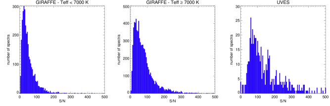
In the observation planning phase we set the requested integration times to aim for a signal-to-noise ratio S/N for a substantial fraction of the O and early B stars. For later-type stars, which contain more spectral lines, we required S/N. For fainter stars, we cannot reach these values within a reasonable integration time, so we aimed for the lower values of S/N for the O and early B stars and S/N for the later-type stars (the corresponding exposure times are listed in Bragaglia et al. 2021). For each of the GIRAFFE setups, the integration times were set to achieve these S/N numbers. The UVES fibres were usually put on brighter targets. As the UVES spectra were taken during the same pointing as the GIRAFFE spectra, their integration time is necessarily the same. The histograms of the obtained S/N are shown in Fig. 1.
| Cluster | log | HR03 | HR04 | HR05A | HR06 | HR09B | HR14A | V mag | U520 | V mag | U580 | V mag | |
| age(yr) | range | range | range | ||||||||||
| 25 Ori | 7.13 | … | … | … | … | … | … | 4 | … | ||||
| Alessi 43 | 7.06 | … | … | … | … | … | … | 13 | … | ||||
| Berkeley 25a𝑎aa𝑎aarchive data | 9.39 | … | … | … | … | 10 | … | … | … | ||||
| Berkeley 25 | … | … | … | … | 71 | … | … | … | |||||
| Berkeley 30 | 8.47 | … | … | … | … | 153 | … | … | … | ||||
| Berkeley 32 | 9.69 | … | … | … | … | … | … | 5 | … | ||||
| Berkeley 81 | 9.06 | … | … | … | … | 118 | … | … | … | ||||
| Collinder 197 | 7.15 | … | … | … | … | … | … | 1 | 7 | … | |||
| Haffner 10 | 9.58 | … | … | … | … | 102 | … | … | … | ||||
| IC 2391 | 7.46 | … | … | … | … | … | … | 11 | 41 | ||||
| IC 2602a𝑎aa𝑎aarchive data | 7.56 | … | … | … | … | … | … | … | 38 | ||||
| IC 2602 | … | … | … | … | … | … | 7 | 95 | |||||
| M 67a𝑎aa𝑎aarchive data | 9.63 | … | … | … | … | … | … | … | 42 | ||||
| NGC 2244 | 6.60b𝑏bb𝑏bage from Bell et al. (2013) | 141 | 36 | 35 | 36 | … | 35 | 29 | 40 | ||||
| NGC 2451 | 7.6c𝑐cc𝑐cage is average of NGC 2451A and NGC 2451B | … | … | … | … | … | … | 4 | … | ||||
| NGC 2516 | 8.38 | … | … | … | … | … | … | 16 | … | ||||
| NGC 2547 | 7.51 | … | … | … | … | … | … | 25 | … | ||||
| NGC 3293a𝑎aa𝑎aarchive data | 7.01 | 106 | 106 | 106d𝑑dd𝑑dHR05B | 106 | … | 106e𝑒ee𝑒eHR14B, | 5 | … | ||||
| NGC 3293 | 522 | 112 | 524 | 523 | 288 | 518 | 22 | … | |||||
| NGC 3532 | 8.60 | … | … | … | … | 150 | … | 18 | … | ||||
| NGC 3766 | 7.36 | 391 | … | 392 | 390 | … | 390 | 8 | … | ||||
| NGC 4815 | 8.57 | … | … | … | … | 113 | … | … | … | ||||
| NGC 6005 | 9.10 | … | … | … | … | 222 | … | … | … | ||||
| NGC 6067 | 8.10 | … | … | … | … | 312 | … | 15 | … | ||||
| NGC 6253a𝑎aa𝑎aarchive data | 9.51 | … | … | … | … | 188 | 199 | … | 91 | ||||
| NGC 6253 | … | … | … | … | … | … | … | 11 | |||||
| NGC 6259 | 8.43 | … | … | … | … | 173 | … | … | … | ||||
| NGC 6281 | 8.71 | … | … | … | … | 78 | … | 5 | … | ||||
| NGC 6405 | 7.54 | … | … | … | … | 52 | … | 12 | … | ||||
| NGC 6530 | 6.30b𝑏bb𝑏bage from Bell et al. (2013) | 11 | … | 11 | 12 | … | 12 | 46 | 16 | ||||
| NGC 6633a𝑎aa𝑎aarchive data | 8.84 | … | … | … | … | 103 | … | 4 | … | ||||
| NGC 6633 | … | … | … | … | 33 | … | 36 | … | |||||
| NGC 6649 | 7.85 | 53 | … | 53 | 53 | 112 | 53 | 5 | 4 | ||||
| NGC 6705 | 8.49 | 166 | 167 | 166 | 166 | 166 | 166 | 10 | … | ||||
| NGC 6709 | 8.28 | … | … | … | … | 123 | … | 10 | … | ||||
| NGC 6802 | 8.82 | … | … | … | … | 108 | … | … | … | ||||
| Pismis 15 | 8.94 | … | … | … | … | 108 | … | … | … | ||||
| Pismis 18 | 8.76 | … | … | … | … | 51 | … | … | … | ||||
| Pleiadesa𝑎aa𝑎aarchive data | 7.89 | … | … | … | … | … | … | … | 23 | ||||
| Carina Neb.f𝑓ff𝑓fCarina Nebula = in the direction of Trumpler 14 (log age = 7.80), Trumpler 15 (6.95), Trumpler 16 (7.13), and Collinder 228 (6.83 - from WEBDA https://webda.physics.muni.cz/) | 6.8-7.8f𝑓ff𝑓fCarina Nebula = in the direction of Trumpler 14 (log age = 7.80), Trumpler 15 (6.95), Trumpler 16 (7.13), and Collinder 228 (6.83 - from WEBDA https://webda.physics.muni.cz/) | 876 | 873 | 874 | 874 | … | 862 | 23 | 22 | ||||
| Trumpler 20a𝑎aa𝑎aarchive data | 9.27 | … | … | … | … | 884 | … | … | … | ||||
| Trumpler 23 | 8.85 | … | … | … | … | 97 | … | … | … |
The clusters that were analysed by WG13 are listed in Table 2. The table shows the number of spectra that are available for each cluster (split up according to GIRAFFE and UVES setup). We also list the V magnitude range covered for each cluster. This range can be quite different from one cluster to another, depending on the distance of the cluster and the range that covers the spectral types we analyse in WG13. For some clusters the data collected by the GES were supplemented by archive data taken with the same instrument in (nearly) the same setups. These spectra were also processed by the GES data reduction pipelines, thus allowing a comparison between the results of our procedure and values published in the literature.
The cluster selection is described in full in Randich et al. (2022), and an overview is given in Bragaglia et al. (2021). Here we provide a short summary relevant to the WG13 work. To select the young clusters with massive stars a longlist was made of clusters that include a large number of OB stars, according to the WEBDA666http://webda.physics.muni.cz database. From this longlist, clusters were dropped if they were too compact, too extended, or too faint for FLAMES, or if other researchers were already collecting FLAMES data. The cluster NGC 3293 was specifically chosen to allow a comparison of our results with one of the well-studied clusters in the literature (Evans et al. 2005). From the remaining clusters a further reduction had to be made to fit within the allotted observing time. This resulted in eight clusters containing massive stars (their names are indicated in italics in Table 2). These were observed with the HR03, HR05A, HR06, and HR14A GIRAFFE setups, and sometimes with the HR04 and HR09B GIRAFFE setups, and with the UVES 520 setup, and in some cases with the UVES 580 setup.
The selection procedure for the stars in each cluster is detailed in Bragaglia et al. (2021). Again, we summarise the WG13 relevant parts here. The stars to be observed in the young clusters with massive stars were selected on the basis of their photometry. A colour-magnitude diagram was used to find the stars that are high-probability members of the cluster; we note that these selections were made before the Gaia data became available. The brightest stars on the main sequence, or on the turn-off of the main sequence, were observed with the UVES fibres; a selection of the fainter ones were observed with the GIRAFFE fibres. None of the cluster member selection criteria are perfect and it is therefore always possible that some of the stars we studied are either fore- or background objects.
Additionally, young clusters with no massive stars, or only a few, were selected. We also selected a number of intermediate-age clusters that contain late B and A-type stars. These were mostly observed with the GIRAFFE HR09B setup for the brighter stars, which are typically located at the cluster turn-off, and HR15N for the fainter ones. These fainter stars are expected to be of a later spectral type, and were therefore not analysed by WG13. As the selection of the stars is based on photometric criteria, it can happen that the HR09B data contain spectral types later than A. For these less massive clusters and intermediate-age clusters, both colour-magnitude diagrams and proper-motion data were used to select cluster member candidates (see Bragaglia et al. 2021). The proper motion data are mainly from SPM4 (Girard et al. 2011) and UCAC4 (Zacharias et al. 2013). If the cluster contains a red clump, the UVES fibres were set on those stars, and the GIRAFFE fibres on the main sequence and turn-off of the main sequence.
In addition to the cluster stars, WG13 also analysed a number of benchmark stars. GES uses benchmark stars to ascertain the accuracy of the stellar parameters determined by the different analysis techniques. For the cooler stars, these benchmarks are stars that have their parameters derived by methods independent of spectroscopy, such as the use of interferometric angular diameters, parallaxes, and bolometric fluxes (Heiter et al. 2015; Jofré et al. 2014, 2018). For hot stars no such standards are available. Instead, the benchmark stars consist of a number of selected stars that have detailed spectral analyses in the literature. The stars used in GES are listed in Table 3, which extends Table 6 of Pancino et al. (2017).
The spectra were sky subtracted and wavelength calibrated (including barycentric correction) by WG7 (GIRAFFE, Gilmore et al. 2022; UVES, Sacco et al. 2014). The data delivered by WG7 also contain the inverse variance spectra, thus providing signal-to-noise ratio information for each wavelength bin.
While GES was not specifically designed to search for binaries, it does include a number of multi-epoch observations for many of the sources. Usually, two sequential integrations were made for each combination of pointing and setup. Additionally, some or all of these pointing–setup combinations were repeated at a later date. In principle, quite a number of sources therefore have multi-epoch data, although the epochs may have been taken during the same night. These multi-epoch data were combined by WG7 into a single spectrum per source. This combination was done after measuring the radial velocities on the individual spectra, both for GIRAFFE spectra (Gilmore et al. 2022, their Sect. 7) and UVES spectra (Sacco et al. 2014, their Sect. 5). The latter paper also discusses the stability of the UVES instrument, while Jackson et al. (2015) does the same for the GIRAFFE instrument. Many of the analyses discussed in this paper were performed on these combined spectra. One exception is the Liège Node, which recombined the multi-epoch data into nightly spectra for their analysis (Sect. 3.5.1), and for the search for SB1 binaries (Sect. 3.5.4). While ROBGrid used the combined spectra for the analysis, they also searched for SB1 binaries based on the multi-epoch data (Sect. 3.2.3).
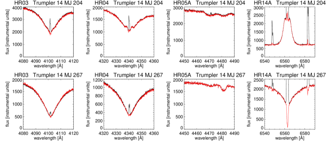
For those clusters where we have H observations, we clearly detect nebular absorption or emission in all stars of the six youngest clusters (i.e. those with an age up to log age(yr) ). It is not seen in H or H, except for the Carina Nebula region, and for about two-thirds of the stars in NGC 6530. In most cases these nebular lines could be handled by masking out the affected wavelength regions in the analysis. In the Carina Nebula, however, the nebulosity is much stronger and also changes as a function of position. The gas responsible for the nebulosity has a complex velocity structure caused by different expanding shells (Walborn et al. 2002) that is seen in the data. For the Carina Nebula another approach was therefore taken: we placed a nebular fibre 10″ away from each star, but since it is not possible to do so in the same exposure777The minimum button separation of the FLAMES Fibre Positioner is 11″ (Kaufer et al. 2011)., we resorted to an on/off strategy with two setups. In the first setup, half of the fibres were allocated to a first set of stars and half were allocated to the sky with a 10″ offset of a second set of stars. In the second setup (the same as the first, but with a global displacement of 10″) the role of each fibre was reversed.
Armed with a sky fibre for each star, our original idea was to directly subtract from each stellar spectrum the corresponding nebular spectrum 10″ away. This turned out to be sufficient for many cases, but not for all, due to the variation of nebular structures even within 10″ and possibly also due to the variations in seeing between the two setups. To solve this problem, we developed an interactive tool that allowed us to introduce slight variations in the intensity and velocity of the nebular fibre spectrum before subtracting it from the stellar spectrum. The subtraction can be done visually because some lines ([N ii] 6548, 6584) are only of nebular origin and can be used as a subtraction template. With the help of this tool we were able to successfully subtract the nebular component for most of the cases (see Fig. 2 for two examples), but a few were left where the nebular contamination could not be fully subtracted. Specifically for H, significant residual negative fluxes remained in the core of the line for % of the stars. For H and H, the situation was much better, with only two stars each having residual negative fluxes. In these cases, one would have to resort to other methods, for example long-slit spectroscopy (Sota et al. 2011), to adequately subtract the nebulosity, but this approach is beyond the scope of GES. The problematic spectra were left in GES and we compensated as much as possible for the presence of residual nebular emission by masking out the affected wavelength regions in the analysis.
3 Analysis
3.1 Overview
The analysis of the hot-star spectra in WG13 follows the same principles as that of the cool spectra in WG10 and WG11 (Smiljanic et al. 2014; Worley et al. 2022): a number of groups (called Nodes) each analyse the spectra independently. The results are then compared and a homogenisation procedure is applied, giving a single set of parameters and abundances for each star (the recommended values). The approach using multiple Nodes is very much needed in WG13, as the temperature range covered is large ( K). To date, no spectrum synthesis code can fully cover this range, and most Nodes are therefore limited to a part of the temperature range (see Table 4). Many of the WG13 Nodes focus on the hotter stars. Where Nodes overlap we can compare the results and thus determine the uncertainty on the stellar parameter determination.
The different analysis techniques used by the Nodes can be roughly divided into two categories. The first technique uses carefully selected sets of diagnostic photospheric spectral lines. The stellar parameters are determined with radiative transfer calculations that fit the profiles of neutral and ionic Fe lines in detail (this applies to the cooler part of the range covered by WG13). The stellar parameters are used to determine the abundances with fits to selected lines of other elements. The second technique uses a comparison of the observed spectrum to theoretically generated ones. In the comparison, all fluxes can have equal weight, or some spectral regions or lines can be favoured over others.
To give an idea of the diverse range of stellar parameters and Node techniques, we present in Appendix A some selected examples of spectra and their best-fit theoretical spectrum or the best fit to specific spectral lines. Figure 13 shows the results for the GIRAFFE data, Fig. 14 for the UVES data.
As part of the data analysis, the Nodes can also flag the spectra to indicate possible problems with the data reduction (e.g. bad normalisation) or with the analysis of the spectrum (e.g. spectral type outside the range of temperature that the Node can handle), or to describe interesting features of the spectrum (e.g. binarity). More details of the flagging are given in Gilmore et al. (2022).
The sections below describe how each Node determines the stellar parameters and abundances. For an overview we provide Table 4, which gives the effective temperature range covered by each Node, the spectral analysis technique used, the derived stellar parameters, and the elements for which abundances are determined. It also provides the references to the atomic data that were used. Table 5 gives the typical uncertainties for the parameters and abundances derived by the Nodes.
| Star | V | Spectral | log | [Fe/H] | |
|---|---|---|---|---|---|
| mag | type | (K) | (cm s-2) | ||
| HD 93128111111Holgado et al. (2020) | 6.90 | O3.5 V | 49 300 | 4.10 | (sol.) |
| HD 319699222222Holgado et al. (2018) | 9.63 | O5 V | 41 200 | 3.91 | (sol.) |
| HD 163758111111Holgado et al. (2020) | 7.32 | O6.5 Iafp | 34 600 | 3.28 | (sol.) |
| HD 462022,3232,32,3232,3footnotemark: | 8.19 | O9.2 V | 34 900 | 4.13 | (sol.) |
| HD 68450111111Holgado et al. (2020) | 6.44 | O9.7 II | 30 600 | 3.30 | (sol.) |
| $θ$ Car4,5454,54,5454,5footnotemark: | 2.76 | B0 Vp | 31 000 | 4.20 | (sol.) |
| $τ$ Sco4,5,6,7,8,94567894,5,6,7,8,94,5,6,7,8,94567894,5,6,7,8,9footnotemark: | 2.81 | B0.2 V | 31 750 | 4.13 | |
| V900 Sco10,11101110,1110,11101110,11footnotemark: | 6.38 | B0.7 Ia | 22 850 | 2.68 | |
| $γ$ Peg4,6,1246124,6,124,6,1246124,6,12footnotemark: | 2.84 | B2 IV | 22 350 | 3.82 | |
| HD 3591213,14131413,1413,14131413,14footnotemark: | 6.38 | B2 V | 18 750 | 4.00 | |
| 67 Oph11,15,16,171115161711,15,16,1711,15,16,171115161711,15,16,17footnotemark: | 3.93 | B5 Ib | 15 650 | 2.68 | |
| HD 56613444444Lefever et al. (2010) | 7.21 | B8 V | 13 000 | 3.92 | … |
| 134 Tau181818181818Smith & Dworetsky (1993) | 4.87 | B9 IV | 10 850 | 4.10 | |
| $o$ Peg171717171717Prugniel et al. (2011) | 4.78 | A1 IV | 9373 | 3.73 | |
| 68 Tau191919191919Burkhart & Coupry (1989) | 4.31 | A2 IV | 9000 | 4.00 | |
| 32 Gem202020202020Gray et al. (2001) | 6.47 | A9 III | 7240 | 2.14 |
, , $3$$3$footnotetext: Sota et al. (2014), , $5$$5$footnotetext: Hubrig et al. (2008), $6$$6$footnotetext: Nieva & Przybilla (2012), $7$$7$footnotetext: Simón-Díaz et al. (2006), $8$$8$footnotetext: Mokiem et al. (2005), $9$$9$footnotetext: Martins et al. (2012), $10$$10$footnotetext: Crowther et al. (2006), $11$$11$footnotetext: Thompson et al. (2008), $12$$12$footnotetext: Morel & Butler (2008), $13$$13$footnotetext: Simón-Díaz (2010), $14$$14$footnotetext: Nieva & Simón-Díaz (2011), $15$$15$footnotetext: Searle et al. (2008), $16$$16$footnotetext: Maíz Apellániz et al. (2018), , , , .
| Sect. | Node | range | Technique | Parameters determined | Abundances |
|---|---|---|---|---|---|
| 3.2 | ROBGrid | K | minimisation with grid | , , [M/H], , a𝑎aa𝑎aWhat is listed here as is actually the total line-broadening parameter, which can include other effects, such as macroturbulence. See Sect. 4.2 for further details. | … |
| of theoretical spectra | |||||
| 3.3 | ROB | K | Fe - Fe+ ionisation balance | , , [Fe/H], , a𝑎aa𝑎aWhat is listed here as is actually the total line-broadening parameter, which can include other effects, such as macroturbulence. See Sect. 4.2 for further details. | C, O, Mg, Al, Sc, Fe |
| of diagnostic photospheric lines | |||||
| 3.4 | MGNDU | K | Principal Component Analysis | , , [M/H] , , | … |
| and Sliced Inverse Regression | |||||
| 3.5 | Liège | K | minimisation with grid | , , , a𝑎aa𝑎aWhat is listed here as is actually the total line-broadening parameter, which can include other effects, such as macroturbulence. See Sect. 4.2 for further details. | He, C, N, Ne, Mg, Si |
| 3.6 | ON | K | Non-LTE synthesis and | , , a𝑎aa𝑎aWhat is listed here as is actually the total line-broadening parameter, which can include other effects, such as macroturbulence. See Sect. 4.2 for further details. | C, O, Si |
| Si ionisation balance | |||||
| 3.7 | IAC | K | minimisation with grid | , , , | He |
| of FASTWIND models | |||||
| 3.8 | Mntp | K | minimisation with grid | , , , | … |
| of CMFGEN models | |||||
| 3.9 | LiègeO | K | CMFGEN | , , , | He, C, N |
| Node | Atomic data for stellar parameters | Atomic data for abundances |
| ROBGrid | Bertone et al. (2008); Munari et al. (2005) | … |
| Coelho et al. (2005); Palacios et al. (2010) | ||
| Lanz & Hubeny (2003, 2007) | ||
| and references therein | ||
| ROB | Kurucz (1992); Castelli & Kurucz (2003) | Laverick et al. (2019) |
| and references therein | ||
| MGNDU | Kurucz (1992); Castelli & Kurucz (2003) | Gebran et al. (2016) and references therein |
| Sbordone et al. (2004) and references therein | ||
| Liège | Lanz & Hubeny (2007) and references therein | He, N, Mg and Si: Morel et al. (2006) and references therein; |
| Ne: Morel & Butler (2008); C: Nieva & Przybilla (2008) | ||
| ON | Hubeny & Lanz (1995, 2017); Bragança et al. (2019) | Bragança et al. (2019) |
| IAC | Puls et al. (2005) and references therein | Puls et al. (2005) and references therein |
| Mntp | CMFGEN websiteb𝑏bb𝑏bhttp://kookaburra.phyast.pitt.edu/hillier/web/CMFGEN.htm | … |
| LiègeO | CMFGEN websiteb𝑏bb𝑏bhttp://kookaburra.phyast.pitt.edu/hillier/web/CMFGEN.htm | CMFGEN websiteb𝑏bb𝑏bhttp://kookaburra.phyast.pitt.edu/hillier/web/CMFGEN.htm |
| Node | [M/H] | Abundances | |||
|---|---|---|---|---|---|
| (K) | (log cm s-2) | (dex) | (km s-1) | (dex) | |
| ROB | 150 – 250 | … | 0.05 – 0.1 | … | 0.05 – 0.1 |
| MGNDU | 150 | 0.35 | 0.15 | 2 | … |
| Liège | 750 | 0.15 | … | 15 | 0.1 – 0.3 |
| ON | 1000 | 0.15 | … | 15% | 0.1 – 0.15 |
| IAC | 1000 | 0.10 | … | 10-20% | … |
| Mntp | 2500 | 0.15 | … | … | … |
| LiègeO | 1000 | 0.1 | … | … | … |
3.2 ROBGrid Node
3.2.1 Grids used
In the ROBGrid Node, we determined the stellar parameters of both GIRAFFE and UVES spectra by comparing them to theoretical spectra from the literature. In selecting these theoretical grids we applied the following criteria: the wavelength range should cover at least 4020 Å – 6850 Å, and the resolving power should be at least 20,000.
We used the following grids: Bertone (Bertone et al. 2008); Munari (Munari et al. 2005); Coelho (Coelho et al. 2005); POLLUX, specifically ATLAS, MARCS_PARALLEL, and MARCS_SPHERICAL (Palacios et al. 2010); TLUSTY_B (Lanz & Hubeny 2007); and TLUSTY_O (Lanz & Hubeny 2003). While some of these grids were calculated with the same atmospheric modelling code (ATLAS), they differ in the line lists used, the mixing length applied, and the radiative transfer code used, among others, and can therefore give different results when we apply them in the fitting procedure. Most of these grids were calculated in local thermodynamic equilibrium (LTE), except TLUSTY_B and TLUSTY_O where both the atmospheric model and the emergent spectrum were calculated in non-LTE. From each of these grids, we prepared a set of rotationally broadened and normalised theoretical spectra covering the various wavelength ranges corresponding to the observed spectra. We limited our choice of theoretical spectra to the set with solar metallicity, and just one set with a higher metallicity and one set with a lower metallicity ([M/H] = 0.3 dex or 0.5 dex, depending on the grid used). This covered the expected metallicity range for Galactic open clusters (see e.g. Netopil et al. 2016).
The use of these grids allowed us to determine the stellar parameters (, , and metallicity, if not too far from solar metallicity) as well as the radial and projected rotational velocities. As the relative element to element abundances that went into these models cannot be changed, in the ROBGrid Node we did not determine abundances of individual elements.
3.2.2 Fitting and normalisation
The fitting code we used in the ROBGrid Node proceeds by comparing each observed spectrum to each rotationally broadened theoretical spectrum. We did not use the radial velocities that were determined by WG8, as the templates they used do not cover the hotter stars well. Instead, we used a cross-correlation technique (David et al. 2014, their Eq. 7) to determine the radial velocity shift, and then calculated the for that comparison. We then determined the stellar parameters (as well as the projected rotational velocity) by the best-fitting theoretical spectrum (minimum ). We further refined the stellar parameters by interpolating the theoretical spectra around the best-fit solution, and again determining which had the minimum . Because we compared the observed spectrum to all possible theoretical spectra from all the literature grids listed above, the minimisation automatically picked the grid to be used. Some grids do not cover the temperature range that is relevant for the given observed spectrum.
The above procedure is part of a larger loop that also includes the normalisation of the observed spectra. The initial normalisation starts by first removing cosmic ray features, and then iteratively fitting a low-order polynomial to the fluxes. In each of these iterations, we remove fluxes that are too different from the polynomial. We then divide this preliminary normalised spectrum into 20 bins. For each bin we explore various levels of the continuum to see at what level the noise of the fluxes above the continuum is consistent with the known signal-to-noise ratio. The final set of 20 data points is then fit with a low-order polynomial, and this provides the initial normalisation. We make a visual check of this normalisation, and apply corrections in the few cases where this is necessary.
In the subsequent steps of the larger loop, we make use of the fact that we have a theoretical spectrum that is in good agreement with the observed spectrum, and for which we know the position of the continuum. We again divide the wavelength range of the spectrum into 20 bins, and for each bin we determine a continuum correction factor, based on the comparison of the average observed spectrum in that bin and the average (normalised) theoretical spectrum. This is then used to fit a low-order polynomial, where we attribute a higher weight to those bins where the average theoretical flux is closer to the continuum. With this updated normalisation, we re-determine the stellar parameters. The loop is then continued until the stellar parameters are sufficiently converged.
We apply the above procedure to the different setups of the GIRAFFE spectra and ensure that the stellar parameters are simultaneously determined for all observed setups of the star. For the UVES spectra we use the data from the separate orders and apply the same procedure. In the normalisation step of the UVES spectra, we handle the orders that contain H and H in a different way, as these lines can be so broad that they extend beyond the order. For these, we determine the continuum by interpolating the continuum of the other orders using a 2D second-order polynomial. This special procedure is not needed for the H line as it is reasonably well centred in its order, which also covers a larger wavelength range. It is not needed for the GIRAFFE spectra either as these also cover a large enough wavelength range.
In the ROBGrid Node we did not have a procedure to determine the uncertainties on the derived stellar parameters. Instead, we assigned the uncertainties that were derived in the homogenisation phase (Sect. 4.3).
3.2.3 Flagging
While processing the data, we also flagged those spectra that have a S/N value that is too low to be analysed, that had problems in the reduction, or that were not possible to normalise or to analyse with ROBGrid. During our visual inspection of how well the model spectra fitted the observations, we also detected double-lined spectra, which we then flagged as potential SB2 binaries.
We also searched for SB1 binaries, using the multi-epoch observations to see if there are significant radial velocity differences between the epochs. For each of the clusters in Table 2, we explored the radial velocity differences between any possible multi-epoch observations of the same GIRAFFE setup. To compare the radial velocities, we cross-correlated the second-epoch spectrum with the first-epoch spectrum. This provided us with the relative radial velocity. To judge how significant this relative radial velocity is, we ran Monte Carlo simulations using the best-fit theoretical spectrum, as determined in Sect. 3.2.2. In the Monte Carlo simulations we shifted the spectrum with a randomly chosen velocity and added noise compatible with the first-epoch observation of that star. Similarly, we made a second spectrum with another randomly chosen velocity and added noise compatible with the second-epoch observation of that star. We then cross-correlated the two simulated spectra, determined the relative velocity, and compared it to the known input relative velocity. We did this for 500 Monte Carlo simulations and then determined the statistical results. The significance of the observed velocity difference can then be judged by comparing it to the standard deviation of the Monte Carlo simulations. For all results above three sigma, we also did a visual inspection and on the basis of this decided whether to flag the star as a potential SB1 binary.
3.3 ROB Node
In the ROB Node, we computed LTE stellar atmosphere models and their resulting spectra, covering a range K. We used Fe i and Fe ii lines to determine the iron ionisation balance and derive the stellar parameters from that. We also determined abundances for six elements (C, O, Mg, Al, Sc, Fe).
Here we give more details of the process. We developed a suite of computer codes for semi-automatic determinations of stellar parameters and abundances in GES, which requires three subsequent major computational steps. First the pre-processor estimates the stellar parameters using a limited number of diagnostic H Balmer, Fe, and Mg absorption lines. The second pipeline step iterates over , surface gravity (), line-of-sight microturbulence velocity (), and metallicity (M/H) until the best fit is obtained to the detailed profiles of a more extensive set of diagnostic photospheric lines: 40 sufficiently unblended Fe i and Fe ii lines with reliable atomic data values of line oscillator strengths, energy levels, and transition rest wavelengths (Lobel et al. 2017). The final step uses the iterated stellar parameters as input to measure the individual element abundances ([X/H]) from selected sets of medium-strong to strong lines (Laverick et al. 2019).
We calculated the theoretical spectra with the LTE radiative transfer code Scanspec101010http://alobel.freeshell.org/scan.html. It iteratively solves the Milne-Eddington transfer equation in 1D stellar atmosphere models (Lobel 2011a). The code is used for the development of the SpectroWeb database at spectra.freeshell.org (Lobel 2008). We included in the calculation important line broadening effects for strong resonance lines and the stellar continua. In addition to atoms, the equation of state also includes important diatomic molecules: a comprehensive set of hydrides; carbon-bearing molecules such as , CN, and CH; and a large number of oxides with updated partition functions. We computed the synthetic spectra using input hydrostatic, plane-parallel atmosphere models that we converge with ATLAS9 (Kurucz 1992). The model calculations adopt the updated opacity distribution functions of Castelli & Kurucz (2003). We adopted a constant mixing-length parameter /H = 1.25 for convection and omitted convective overshoot (as recommended by Bonifacio et al. 2012) and turbulent pressure contributions.
| Parameter | Range | Steps | |
|---|---|---|---|
| (K) | 50 | ||
| (dex) | 0.2 | ||
| [Fe/H] (dex) | 0.1 | ||
| (km s-1) | 0.5 | ||
| (km s-1) | 1 | ||
We calculated a large homogeneous grid of synthetic spectra between 3200 Å and 6800 Å. The parameter space of applicability for the ROB stellar parameter pipeline is provided in Table 6. We adopted the solar chemical composition of Grevesse et al. (2007).
Our suite of computer codes can semi-automatically determine stellar parameters and abundances of A- and late B-type GES spectra. The Mg ii 4481 triplet lines are very temperature sensitive in A-type stars. We used their line equivalent widths (EWs) observed in GIRAFFE spectra to find an initial estimate of . The values of and log were initially varied in steps of 250 K and 0.5 dex, respectively. We measured the EW-value of Mg ii 4481 after rectifying the observed spectrum to a local continuum flux level around the line. The model - and log -values were varied in combination with (in steps of 0.5 km s-1) until the observed EW was found. This yields a series of initial models that we used to calculate the detailed theoretical spectrum around the diagnostic Fe lines.
The ROB parameter determination method was developed according to traditional spectral diagnostic methods using sets of selected Fe i and Fe ii lines to determine the atmospheric iron ionisation balance. It iteratively determines the atmospheric Fe-ionisation balance and guarantees consistency between the metallicity of the atmosphere model and the Fe abundance. The method iterates until the best fit to the continuum-normalised and broadened Fe-line profiles is accomplished using -minimisation. The stellar parameter iterations loop over until [Fe/H] is in agreement with the metallicity of the atmosphere model within the resolution of the ATLAS9 model grid (typically 0.1 dex). The iterations minimise the difference between the abundance values calculated from the diagnostic Fe i and the Fe ii lines. Hence, the best-fit -value is consistent with the Fe- ionisation balance in the final atmosphere model. We convolved the resulting synthetic spectra with the (total) RMS mean of the rotational broadening and macroturbulence velocity values. The latter velocity is not separately determined from the projected rotational velocity. We used the appropriate filter functions that simulate the instrumental resolving power of the various GIRAFFE setups HR03, HR05A, and HR09B and of UVES 520.
We determined from the GES spectra instead of adopting parameterised -values (sometimes derived from and ) as this would be inaccurate for A- and late B-type stars ( K). There is a maximum in around the mid-A stars. We also iterated the -value in steps of 1.0 km s-1 to obtain the best fit to the detailed (broadened) profile shapes of the diagnostic Fe lines. The ROB analysis method of determining A-star parameters from Fe i and Fe ii lines is supported by the fact that the main ionisation stage turns from neutral to ionised iron around 7000 K, allowing for accurate determinations of -values, combined with -values from gravity-sensitive lines.
Based on UVES 520 data, we determined stellar parameters of 63 stars having 6000 11,500 K in five open clusters. Using GIRAFFE spectra, we did the same for an additional 97 stars in NGC 3293 and for 93 stars in NGC 6705 (no UVES data were analysed for NGC 6705). The stellar parameters were then used to determine the detailed abundances of six elements from good-quality UVES 520 spectra. The iron abundance was determined from the GIRAFFE and UVES spectra. The ROB stellar parameters were calculated with uncertainty estimates. Two main sources of uncertainty were accounted for: the S/N ratio in the spectral region of the diagnostic Fe lines, combined with the size of the final parameter- and abundance-value iteration step. The ROB parameter uncertainties range from K for K to K for K. The ROB metallicities and element abundances have uncertainties ranging from 0.05 dex to 0.1 dex, generally exceeding the final abundance iteration step (or best fitting the depth and equivalent line widths) by several factors. All information about the uncertainties is summarised in Table 5.
An interesting result of the ROB analysis is that is maximum around mid-A stars of K. The -maximum has previously been observed in other clusters and field stars (Gebran et al. 2014). The new results for NGC 3293 and NGC 6705 contribute to ongoing investigations into the physics of astrophysical microturbulence. The importance of microturbulence cannot be overstated for accurately determining stellar parameters from stellar spectra (Lobel 2011b; de Jager et al. 1997).
3.4 MGNDU Node
The procedure we follow in the MGNDU Node is based on a combination of principal component analysis (PCA) complemented with a sliced inverse regression (SIR) applied on spectra of B-A-F stars. We start by compiling a learning database using synthetic spectra. ATLAS9 model atmospheres are calculated using the latest version of Kurucz (1992) code (see also Castelli & Kurucz 2003; Sbordone et al. 2004). These 1D plane-parallel models use the new opacity distribution functions and assume LTE and hydrostatic equilibrium. Convection is treated according to the mixing-length theory (MLT) using a ratio of the mixing length to the pressure scale height () of 0.5 for stars with effective temperatures lower than 8500 K and 0 for higher values (Smalley 2004). These model atmospheres are included in the calculation of the synthetic spectra. We used the SYNSPEC48 LTE code of Hubeny & Lanz (1992) complemented with the line list of Gebran et al. (2016).
3.4.1 MGNDU’s learning database
We analysed GES data from the UVES 520 setup. For this reason the learning database was calculated for the wavelength range of 4450–4990 Å. This region harbours many lines that are sensitive to , , [M/H], and . It also includes lines that are insensitive to microturbulent velocity, which was fixed to km s-1 based on the average value for A stars (Gebran et al. 2014, 2016). The parameters that were used for the calculation of the synthetic spectra learning database are displayed in Table 7. All spectra were calculated at the resolving power of 47 000, the resolving power of FLAMES spectra in the UVES 520 setup.
| Parameter | Range | Steps | |
| (K) | 100 | ||
| (dex) | 0.1 | ||
| [M/H] (dex) | 0.1 | ||
| (km s-1) | |||
| … | |||
3.4.2 MGNDU’s derivation of fundamental parameters
In order to derive the fundamental parameters of UVES 520 stars, we start by sorting all the synthetic spectra in the learning database to form the global matrix called . This matrix contains each one having flux points. We then calculate the variance-covariance matrix , having a dimension of and defined as
| (1) |
where is the average of along the axis.
As shown and detailed in Paletou et al. (2015) and Gebran et al. (2016), only the first 12 Principal Components of the symmetric matrix are used as the new basis for the calculations of the synthetic spectra and observation coefficients. Then for each observation, the nearest neighbour is found by minimising the difference between the projected coefficients
| (2) |
where covers the number of spectra in the learning database and and are the projected coefficients in the principal component low dimension space, respectively of the observation and of the -th synthetic spectrum. For this purpose we used the normalised spectra delivered in iDR6 in the UVES 520 setup.
As described in Kassounian et al. (2019), the next step of the procedure is to sort the synthetic spectra by increasing order of the considered parameter for inversion (, , [M/H], ) while keeping the remaining parameters ordered randomly. A subset of spectra are then built up and stacked into slices, having the same (or very close) values of the considered parameter. For the inversion of each parameter, we calculate the intra-slice covariance matrix
| (3) |
where , is the number of spectra in the matrix containing the sorted spectra, and is the slice that contains synthetic spectra.
The matrix is then calculated and its eigenvector corresponding to the largest eigenvalue is considered for the inversion of the considered parameter (see Eq. 9 of Kassounian et al. 2019). The average uncertainties for the inverted parameters are around 150 K, 0.35 dex, 0.15 dex, and 2 km s-1 for , , [M/H], and , respectively (Table 5). No elemental abundances, other than Fe, are determined by MGNDU.
3.4.3 Pre-processing of the UVES 520 spectra
Before inverting the fundamental parameters (, , and [M/H]) and , we corrected all analysed UVES 520 spectra for their radial velocity (). We did not use the available values for these parameters, we instead decided to derive them. It is shown in Paletou et al. (2015) and Gebran et al. (2016) that should be known to an accuracy of , where is the speed of light and the resolving power of the observations. In the case of UVES 520 spectra, should be known to an accuracy of km s-1 in order to properly invert the parameters. Using the classical cross-correlation technique, the radial velocities were determined by comparing the UVES 520 observations with a synthetic template having K, dex, [M/H] dex, and km s-1.
Observations are renormalised according to the procedure described in Gebran et al. (2016). It consists in performing several iterations on each observed spectrum in order to ensure a proper comparison between observations and synthetic data. This procedure was initially used in Gazzano et al. (2010) on FLAMES/GIRAFFE observed spectra in CoRoT/Exoplanet fields.
An example of the fitting PCA/SIR inversion technique is shown in Fig. 14. The inverted parameters for 68 Tau are used to calculate the synthetic spectra that should best fit the observed ones.
3.5 Liège Node
We determined the parameters and chemical abundances of stars in the NGC 3293 cluster and benchmark stars covering the full temperature range of B stars (i.e. from about 10 000 to 32 000 K). Our code is unable to treat stars suffering significant mass loss because our analysis relies on codes assuming plane-parallel atmospheres in hydrostatic equilibrium (see below). This is not a concern for our sample because the stars are neither so massive nor so very evolved that they would have a strong stellar wind. The stars to be processed at the lower boundary were selected by a visual inspection of the blend formed by Ti ii 4468 and He i 4471: the Ti ii feature dominates for A stars.
3.5.1 Pre-processing
We analysed the GIRAFFE and UVES data including those of the warm GES benchmark stars (Table 3). Data taken from the ESO archives obtained in the framework of the VLT-FLAMES Survey of Massive Stars (Evans et al. 2005) were also treated. The HR03, HR04, HR05A/B, HR06, and UVES 520 (lower arm) data were used for the parameter and abundance determination. HR09B was not considered because it does not contain enough information. HR14A/B was only used to estimate the Ne i and Si ii abundances.
The individual exposures of all setups were extracted from the original GES files and grouped into epoch spectra: consecutive exposures were averaged, and spectra obtained over different nights were treated separately. All the spectra were normalised manually with IRAF111111iraf.noao.edu/ using low-order polynomials.
3.5.2 Parameters
We used a method based on a least-squares minimisation to derive the stellar parameters and the radial velocities. We fitted the observed normalised spectra with a grid of solar metallicity, synthetic spectra computed with the SYNSPEC program on the basis of non-LTE TLUSTY (Lanz & Hubeny 2007) and LTE ATLAS (Kurucz 1993) model atmospheres. We used the TLUSTY grid for the early B stars with two different microturbulence values (2 and 5 km s-1) and the ATLAS grid for the late B stars, assuming a microturbulence of 2 km s-1.
The first step of our method consists in determining the radial velocity and projected rotational velocity of all epoch setups. The synthetic spectra are thus rotationally broadened and shifted in velocity. The basic rotational profile used is the standard one (as given by e.g. Gray 2005). We did not consider broadening by macroturbulence, and this could have had some influence on the resulting rotational velocity. However, macroturbulence was not expected to dominate for the kind of objects the Liège Node studied for iDR6 (Simón-Díaz et al. 2017). Both radial velocity and projected rotational velocity quantities were determined with respect to a grid of synthetic spectra spanning a large range of stellar parameters. Then, for each target, we corrected each epoch setup for their individual radial velocity and combined them in one spectrum in the rest wavelength scale.
Finally, the determination of the effective temperature and surface gravity is performed over the whole wavelength domain by finding the best fit between the grid of synthetic spectra convolved with the rotational velocity averaged on the values obtained for each epoch setup and the combined spectra. After determining the effective temperature and the surface gravity, we use these parameters to compute again the radial velocity and projected rotational velocity of the different epoch setups. In these first fits, an uncertainty is associated with each measurement on the basis of the behaviour of the surface. The typical 1 uncertainties are 750 K for the effective temperature, 0.15 dex for the , 15 km s-1 for the projected rotational velocity, and 2 km s-1 for the radial velocity (Table 5).
3.5.3 Abundances
We considered the following species for the abundance analysis: He, C, N, Ne, Mg, and Si (both Si ii and Si iii). We derived the non-LTE abundances by finding the best match in a sense between a grid of rotationally broadened synthetic spectra and the observed line profiles of He i 4471, C ii 4267, N ii 4630, Ne i 6402, Mg ii 4481, Si ii 6371, and Si iii 4568-4575.
For the line modelling we used the non-LTE code DETAIL/SURFACE originally developed by Butler (1984). We refer to Morel et al. (2006) and Morel & Butler (2008) for details about the version of the code currently used and the model atoms implemented. We used synthetic C ii 4267 spectra computed with the carbon model atom of Nieva & Przybilla (2008). A microturbulence, , of 2 km s-1 is assumed for all stars, except for the relatively evolved, early B stars ( 22 000 K and ) for which it is arbitrarily fixed to 5 km s-1. The abundance uncertainties are estimated empirically by comparing the results for stars having multiple determinations from GES and archival data. For early B stars we also take into account the impact of the choice of the microturbulence. The 1 uncertainties on the abundances are typically in the range 0.1-0.3 dex.
3.5.4 Flagging
Along with the Liège Node pre-processing, we applied a first eye inspection of all individual spectra to detect obvious SB2 objects (or objects and spectra presenting clear oddities) that cannot be processed due to their nature. All the other objects were treated according to the processing described in Sect. 3.5.2. In parallel to this determination of the physical parameters, we then scrutinised the deduced radial velocities to detect binaries and/or variable stars through radial velocity variability as a first step. The main part of the work was done on the basis of the distribution over the population of objects of the differences in radial velocities between pairs of setups (we used HR03 versus HR04 and HR03 versus HR05A/B). As a second step, for objects presenting various observations in setups corresponding to the same wavelength domain (including that of UVES 520), we listed the cases of variations within each of these setups. Concomitantly, we visually inspected the corresponding spectra. Stars presenting significant variability on the basis of at least two criteria (i.e. within the same wavelength domain, or one or two of the two pairs) were classified as true variables with a good significance level. An additional visual inspection tended to discriminate between SB1 (or previously unrecognised SB2) and line-profile variables (due to pulsations or to any other cause). Except for well-marked SB1, these objects were rejected from further treatment. For weak or marginally detected variations, the object might not be rejected from the parameter determination process because a weak variation of the profile does not necessarily hamper the parameter determination.
3.6 ON Node
As a first step in the ON Node, we obtained estimates of from He i lines in order to select those stars with reasonably sharp lines and thus suitable for a chemical analysis. The estimates were based on the widths of the He i lines 4388 and 4471 measured from the observed spectra and interpolated in a grid of theoretical widths measured from non-LTE synthetic spectra by Daflon et al. (2007).
For those stars suitable for a photospheric analysis, we adopted the methodology consisting of full non-LTE spectral synthesis using the code SYNSPEC and a new grid of line-blanketed non-LTE model atmospheres calculated with TLUSTY (Hubeny & Lanz 1995, 2017), with updated model atoms that include higher energy levels, instead of the superlevels previously adopted, as described in Bragança et al. (2019). This new grid of model atmospheres comprises models for between and K, in steps of 1000 K, and surface gravity between 3.0 and 4.5 dex, in steps of 0.12 dex. We convolved the theoretical spectra to simulate the broadening by the corresponding instrumental profile plus macroturbulence fixed to 5 km s-1. In our method, spectra with high signal-to-noise ratio are necessary in order to disentangle the effects of macroturbulence, microturbulence, and on the wings of metal lines. Given the typical signal-to-noise ratio of the studied spectra, we elected to fix the macroturbulence velocity.
The analysis is based on GIRAFFE spectra, mainly using the setups HR03 (H and Si ii lines), HR04 (H), HR05A (He i and Si iii lines), HR06 (C iii, O ii, Si iv lines). The line list and the adopted values of oscillator strength are presented in Table 2 of Bragança et al. (2019). We used the normalised spectra provided by the ROBGrid Node as a starting point in the fitting procedure, although some pieces of spectra were re-normalised, when needed, by fitting a low-order polynomial.
The self-consistent analysis starts with the fitting of hydrogen lines in order to define the pairs of parameters and that can reproduce the observed H profiles. We then use the ionisation balance of Si ii-Si iii-Si iv, when possible, to constrain the effective temperature. We derive the abundances of C, O, and Si for a range of values of microturbulence velocity , which is then fixed from a plot of elemental abundances versus line intensity (equivalent widths), requiring that the abundance is independent of line strength. The elemental abundances, radial velocities and are varied in order to get the best fit for different spectral regions independently. We used the recommended values of radial velocities and provided by the WG8 as starting values in the fitting procedure and the best fits were chosen by minimisation. The final stellar parameters and elemental abundances are represented by the average and dispersion computed from the fits of individual spectral lines or regions.
The adopted iterative scheme yielded individual parameters with uncertainties K, , % of , and km s-1. We estimated the impact of these uncertainties on the derived abundances by changing the individual stellar parameters one at a time and adding the abundance variations in quadrature. The abundance uncertainties vary from 0.10 dex to 0.15 dex, with the highest impact caused by and microturbulence.
3.7 IAC Node
We analysed the early-type OB star sample in the Carina Nebula region (excluding detected SB2 binaries), as well as the earliest benchmark stars, by using semi-automatised tools for the determination of the physical stellar parameters based on large grids of synthetic spectra computed with the non-LTE FASTWIND stellar atmosphere code (Santolaya-Rey et al. 1997; Puls et al. 2005). Our grid of models covers the wide range of stellar and wind parameters considered for standard OB-type stars, from early O to early B types and from dwarf to supergiant luminosity classes (see Table 12). We used the spectra as normalised by the ROBGrid Node and the radial velocities determined by WG8.
| Parameter | Range or specific values | Step |
|---|---|---|
| [K] | 1000 | |
| log [dex] | 0.1 | |
| log | … | |
| (He) | … | |
| [km s-1] | 5 | |
| 0.2 |
3.7.1 Line-broadening characterisation
We first used the iacob-broad tool (Simón-Díaz & Herrero 2007, 2014), a procedure for the line-broadening characterisation based on a combined Fourier transform plus a goodness-of-fit methodology that allows the stellar projected rotational velocity () and the amount of non-rotational broadening (known as macroturbulent broadening, ) to be determined in OB-type stars. We mainly based the analysis on the Si iii 4552 line since metallic lines do not suffer from strong Stark broadening nor from nebular contamination. However, for the few cases where this line is too weak we used nebular free or weakly contaminated He i lines (He i 4713, 4471 and/or 4387, see Ramírez-Agudelo et al. 2013; Berlanas et al. 2020). Typical uncertainties in and are of the order of 10 – 20.
3.7.2 Determination of the fundamental parameters
Both and parameters along with the normalised observed spectrum are mandatory inputs for the user-friendly iacob-gbat tool (Simón-Díaz et al. 2011). Using optical H and He lines allows it to accurately determine the main fundamental stellar parameters such as the effective temperature (), surface gravity (log ), helium abundance ((He), defined as ), microturbulence (), wind-strength parameter131313The parameter combines the mass-loss rate , the terminal velocity of the wind , and the stellar radius . It is defined as (Puls et al. 1996). (), and the exponent of the wind velocity-law141414The stellar wind material presents a velocity law with a exponent dependency: , where represents the photospheric stellar radius of the star. (). If additional stellar information (the absolute visual magnitude and/or the terminal velocity) is provided, this tool also computes other physical stellar parameters, such as the radius (), the luminosity (), the mass (), and/or the mass-loss rate (). For a recent use of the tool see Holgado et al. (2018). We considered the following diagnostic lines for the analysis of the sample: H, H, H, He i 4387, He i 4471, He i 4713, He i 6678, He ii 6683, He ii 4541, and He ii 4686. Basically, once the observed spectrum is processed, the tool compares the observed and the synthetic line profiles by applying a algorithm, and then estimates the goodness of fit for each model within a subgrid of models selected from the global grid. The given parameters are the mean values computed from the models located within the 1 confidence level of the total distributions. Then the associated uncertainties are given by the standard deviation within the 1 level (see Simón-Díaz et al. 2011, for further details). Typical uncertainties are of the order of 1000 K, 0.10 dex, 0.15 dex, and 0.03 in , log , log , and Y (He), respectively (Table 5). An example of the best-fitting model is shown in Fig. 13.
However, we found two stars (Tr14 MJ-190 and Tr16 MJ-224) for which the He ii signal is too low to use this methodology. In these cases, due to the good agreement between temperatures determined using Si ii-iii-iv lines and the He i-ii ionisation balance (Simón-Díaz 2010), we carried out an analysis based on equivalent widths (EW) of silicon lines, similar to the method used by Berlanas et al. (2018). The two parameters, and log , were iteratively obtained by comparing the EW ratios of Si iii 4552/Si iv 4116 or Si ii 4130/Si iii 4552 (depending on the temperature of each star) and the wings of the H Balmer lines with our grid of FASTWIND stellar atmosphere models.
3.8 Mntp Node
We used the non-LTE code CMFGEN (Hillier & Miller 1998) for the spectroscopic analysis of stars in the Carina Nebula region, as well as the earliest benchmark stars. We started from the normalised spectra as delivered by the ROBGrid Node. We relied on a pre-computed grid of models and synthetic spectra that cover the full range of stellar parameters for O stars.
The determination of effective temperatures and surface gravities is performed as follows. We first determine the projected rotational velocity of each star by computing the Fourier transform of Si iii 4552 and/or He i 4713. The position of the first zero is associated with , as described by Simón-Díaz & Herrero (2014).
We then estimated the effective temperature and surface gravity of the star from its spectral type, using the calibration of Martins et al. (2005). We then selected a synthetic spectrum from our grid with the same temperature and gravity. We convolved this spectrum with a rotation profile with the value determined previously. Convolution with a Gaussian profile to take into account the instrumental resolution is also made. We added a third level of convolution, using a radial-tangential profile assumed to represent macroturbulence. Several values of were used. Comparison of the final theoretical profile with the observed Si iii 4552 and/or He i 4713 lines then yields .
In a third step, we convolved our entire theoretical spectral library with the determined and (and instrumental dispersion). We compared each individual convolved spectrum with the observed spectrum, using the radial velocity we determined. In practice, we focused on spectral features sensitive to both effective temperature and surface gravity: H, H, H, He i 4387, He i 4471, He ii 4542, and He ii 4686. We assessed the fit quality by means of a analysis. We adopted the effective temperature and surface gravity of the model with the smallest as the final stellar parameters. We renormalised all values to the minimum (), and estimated the 1 uncertainties from the contours +1. Typical uncertainties on and are 2500 K and 0.15 dex (Table 5).
| Cluster | ROBGrid | ROB | MGNDU | Liège | ON | IAC | Mntp | LiègeO | |
| 25 Ori | 3 | … | … | … | … | … | … | … | |
| Alessi 43 | 6 | … | … | … | … | … | … | … | |
| Berkeley 25a𝑎aa𝑎aarchive data. | 9 | … | … | … | … | … | … | … | |
| Berkeley 25 | 23 | … | … | … | … | … | … | … | |
| Berkeley 30 | 92 | … | … | … | … | … | … | … | |
| Berkeley 32 | 1 | … | … | … | … | … | … | … | |
| Berkeley 81 | 89 | … | … | … | … | … | … | … | |
| Haffner 10 | 100 | … | … | … | … | … | … | … | |
| IC 2391 | 37 | … | 8 | … | … | … | … | … | |
| IC 2602a𝑎aa𝑎aarchive data. | 33 | … | … | … | … | … | … | … | |
| IC 2602 | 97 | … | 4 | … | … | … | … | … | |
| M 67a𝑎aa𝑎aarchive data. | 40 | … | … | … | … | … | … | … | |
| NGC 2244 | 274 | … | 19 | … | … | … | … | … | |
| NGC 2451 | 3 | … | 4 | … | … | … | … | … | |
| NGC 2516 | 12 | 11 | 16 | … | … | … | … | … | |
| NGC 2547 | 21 | 15 | 24 | … | … | … | … | … | |
| NGC 3293a𝑎aa𝑎aarchive data. | 504 | … | … | 330 | … | … | … | … | |
| NGC 3293 | 1079 | 215 | … | 366 | 15 | … | … | … | |
| NGC 3532 | 160 | … | 15 | … | … | … | … | … | |
| NGC 3766 | 902 | … | … | … | … | … | … | … | |
| NGC 4815 | 78 | … | … | … | … | … | … | … | |
| NGC 6005 | 161 | … | … | … | … | … | … | … | |
| NGC 6067 | 305 | … | 9 | … | … | … | … | … | |
| NGC 6253a𝑎aa𝑎aarchive data. | 451 | … | … | … | … | … | … | … | |
| NGC 6253 | 10 | … | … | … | … | … | … | … | |
| NGC 6259 | 169 | … | … | … | … | … | … | … | |
| NGC 6281 | 80 | … | 3 | … | … | … | … | … | |
| NGC 6405 | 59 | … | 7 | … | … | … | … | … | |
| NGC 6530 | 85 | 10 | 15 | … | … | … | … | … | |
| NGC 6633a𝑎aa𝑎aarchive data. | 102 | … | 4 | … | … | … | … | … | |
| NGC 6633 | 64 | 22 | 33 | … | … | … | … | … | |
| NGC 6649 | 276 | … | 3 | … | … | … | … | … | |
| NGC 6705 | 653 | 244 | 10 | … | … | … | … | … | |
| NGC 6709 | 129 | … | 8 | … | … | … | … | … | |
| NGC 6802 | 82 | … | … | … | … | … | … | … | |
| Pismis 15 | 81 | … | … | … | … | … | … | … | |
| Pismis 18 | 50 | … | … | … | … | … | … | … | |
| Pleiadesa𝑎aa𝑎aarchive data. | 23 | … | … | … | … | … | … | … | |
| Carina Neb. | 1625 | … | 4 | … | 169 | 268 | 55 | 293 | |
| Trumpler 20a𝑎aa𝑎aarchive data. | 606 | … | … | … | … | … | … | … | |
| Trumpler 23 | 93 | … | … | … | … | … | … | … | |
| Benchmarks | 479 | 11 | 18 | 148 | 21 | 30 | 19 | … |
3.9 LiègeO Node
We used the CMFGEN non-LTE atmosphere code to determine the physical parameters of the O- and early B-type stars in the Carina Nebula region. The spectra were carefully normalised by fitting polynomials of degree 3 or 4 (depending on the wavelength range) to carefully chosen continuum windows. Before determining the stellar parameters of the stars, we first tag all the stars that present binarity. For this purpose, we look for double signatures in the observed spectra, and also asymmetries that can be related to the presence of a companion. Finally, we measure the radial velocities on the lines with a same ionisation stage (mainly He i) among the different setups. All the stars detected as binaries were removed from our sample.
For the determination of the stellar parameters, the methodology of our study is the same as described by the Mntp Node (Sect. 3.8). We determined the and by using the iacob-broad tool described by Simón-Díaz & Herrero (2014). We built a grid of CMFGEN models covering the effective temperature range between 27 000 K and 46 000 K, with steps of 1000 K, and the surface gravity range from 3.0 to 4.3 dex, with steps of 0.1 dex. The luminosity was calibrated from Martins et al. (2005) to compute the models. For these models, we used Vink et al. (2000, 2001) for the mass-loss prescriptions. The terminal wind velocities were fixed to 2.6 times the effective escape velocity from the photosphere, and for the acceleration of the wind outflow we used . For each object, the synthetic spectra were convolved a first time with the rotation profile and then a second time with a radial-tangential profile to take the into account. Once convolved by the different effects, we shifted these spectra in radial velocity and compared them to the observations to constrain the and of the stars. The quality of the fit was quantified by means of a analysis. The was computed for each model of the grid and we interpolated between these points with a step of K and . The uncertainties at 1, 2, and 3 on and are estimated from , 6.18, and 11.83, respectively (two degrees of freedom, Press et al. 2007).
To estimate the effective temperatures, we used the ionisation balances between He i and He ii lines for the O-type stars (mainly He i+ii 4026, He i 4389, He i 4471, He i 4713, He ii 4200, and He ii 4542) and between Si iii and Si iv for early B-type stars (mainly Si iii 4552, Si iv 4089, and Si iv 4116). For the latter, we also used the balance between the He i 4471 and the Mg ii 4481 lines as a second diagnostic. The typical uncertainty on the effective temperature is about 1000 K. The surface gravities were determined from the wings of the Balmer lines (H and H), giving typical uncertainties of about 0.1 dex (Table 5).
To determine the surface abundances we used the method described by Martins et al. (2015) and Mahy et al. (2020), with fixed and . While the helium abundance is solar for all our stars within the uncertainties, we focused on the carbon (e.g. C iii 4068-70), and nitrogen (e.g. N iii 4097, N iii 4197, N iii 4379, N iii 4508-12-15-20) lines by carefully selecting lines present within the GIRAFFE or UVES wavelength range. As mentioned by Martins et al. (2015), more accurate estimations of the surface abundances can be provided when all the lines are fitted at the same time. Preferably, we selected lines of the same element at different ionisation stages, but we were limited by the spectral range of our data. The uncertainties on the surface abundances depend on the number of diagnostic lines and the signal-to-noise ratio of the analysed spectrum.
3.10 Nodes summary
4 Stellar parameters
4.1 Benchmark stars
We first discuss the ROBGrid results for the benchmark stars. ROBGrid has only a limited range of metallicities ( to dex for most of the grids it uses; to dex if the 0.3 dex is not present in the grid). As may be expected, a comparison with benchmark stars that have metallicities well beyond this range shows large differences in the derived stellar parameters. We therefore limit the further analysis of the ROBGrid benchmarks to those with metallicities in the to range. As WG13 processes only the hotter stars, we also introduce a lower limit cutoff on . While the formal limit for WG13 is 7000 K, we set the limit at 6000 K to ensure some overlap with the other working groups. Details of these cooler benchmark stars are given in Pancino et al. (2017). We also include the Sun in the analysis.
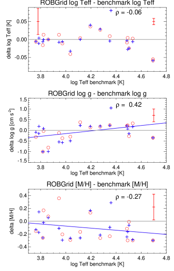
Figure 3 shows the differences between the ROBGrid values and the reference values for the benchmark stars. The top panel shows the differences, the middle panel the differences, and the bottom panel the metallicity differences. The agreement with is acceptable, but some systematic offset between the ROBGrid and metallicity values and the reference values is seen. We therefore decided to apply a correction to all ROBGrid and metallicity values before they enter the homogenisation phase.
The correction is based on a linear fit of the differences (in the sense ROBGrid minus reference values) against . Multiple values for the stellar parameters are determined by ROBGrid, as there are multiple spectra available. To avoid some benchmark stars having a greater weight in the fitting, the average of the ROBGrid stellar parameter values is used. All data from GIRAFFE, UVES 520, and UVES 580 are combined. The linear fit coefficients are then used to correct the ROBGrid values of and metallicity before they are used in the homogenisation. The slope of the correction is significantly different from zero (slope = , and correlation coefficient ), but that of the metallicity is only marginally different from zero (slope = , ). Nevertheless, we opted to keep the linear correction for both parameters. We also explored linear fits separately for the GIRAFFE data and the UVES 520 and 580 data, but these gave nearly identical results.
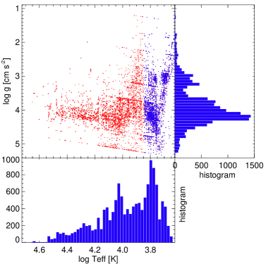
An overview of the ROBGrid data in the form of a Kiel diagram is shown in Fig. 4. Cool stars ( K) are indicated separately (in blue); although ROBGrid did determine stellar parameters for these stars, the code used is less appropriate for that temperature range. During the homogenisation procedure applied by WG15 (Hourihane et al. 2022), preference for these cool stars is given to results from other WGs. The figure also shows the histograms of and , giving a good indication of the data that have been processed by WG13.
The other Nodes processed only a limited number of benchmark stars. The agreement in for these Nodes is generally very good. The determination of is more challenging, with some Nodes having offsets of 0.3 dex, or more. As these offsets are not systematic, the application of corrections for these Nodes is not warranted. For the metallicity, many Nodes assume the solar value, which is indeed appropriate for the hottest stars. The only cooler star analysed by some of the other Nodes is Procyon; its benchmark metallicity is listed in Pancino et al. (2017, their Table 4). Nodes that allow for non-solar metallicities find good agreement with the benchmark reference values. The details of the comparison between the other Nodes and the benchmark stars are presented in Table 12.
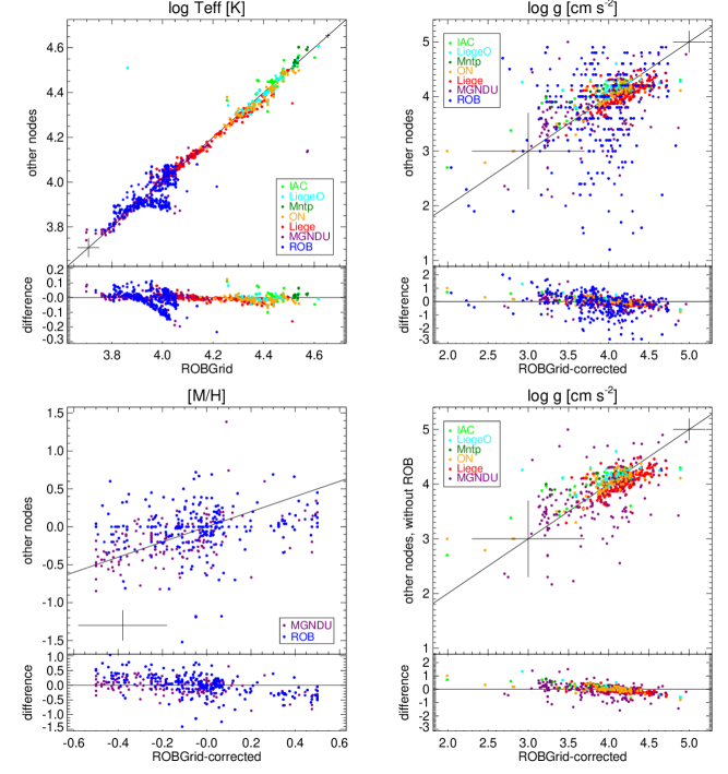
4.2 Comparison between Nodes
Figure 5 shows a comparison between the results of the ROBGrid Node and those of the other Nodes. This comparison covers all of the cluster stars, as well as the benchmark stars, where there is overlap with the ROBGrid Node. The ROBGrid values for and metallicity are the corrected ones (Sect. 4.1). The top left panel shows that agreement in is usually very good, with just a few outliers. There is a striking feature around on the ‘other Nodes’ axis: there is a lack of stars with effective temperature around that value. This is most prominent in the ROB results, but it is also present in the MGNDU results, while ROBGrid does not show such a feature. We suspect this problem is due to the Balmer lines, which reach their maximum strength around this . Because they are sensitive to both and , it is possible that one dependency is compensated by a change in the other when trying to find the best fit. This compensation works differently in different techniques, and could therefore lead to a stagnant and a corresponding spread in for some Nodes.
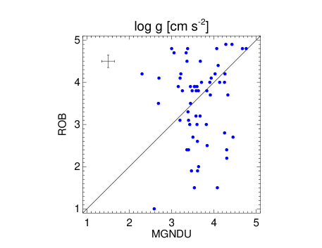
The top right panel of Fig. 5 compares the values showing a large spread in the results. This is not surprising as determining from spectroscopic data is notoriously difficult. As the spread is mainly due to the ROB values, we also plot them as a function of the MGNDU values (Fig. 6) as these two Nodes have a large overlap. Again, a large spread in the values is present with no clear systematics in the behaviour. Various tests were made to find out the reason for these differences. They are mainly related to the different approaches taken by the two Nodes. ROB uses the Fe ionisation equilibrium, while MGNDU uses a full spectrum synthesis (as does ROBGrid), which also includes the hydrogen lines. As mentioned above, the stagnant would also lead to a spread in . If we leave out the ROB values (bottom right panel of Fig. 5), we still find a large spread in values, but it is still reasonably symmetric around the diagonal. The Liège data show a small offset: ROBGrid values are a bit higher than the Liège ones. The other remaining Nodes are in acceptable agreement with ROBGrid.
Besides ROBGrid, only two other Nodes determine metallicities: ROB and MGNDU. For the purpose of that comparison, we do not distinguish between metallicity ([M/H]) and iron abundance ([Fe/H]). The lower left panel of Fig. 5 shows that the MGNDU metallicities are in acceptable agreement with the ROBGrid ones, though with a hint of a small downward-sloped gradient in the difference plot, and with a number of outliers. The comparison between ROBGrid metallicity and ROB Fe abundance shows a larger scatter.
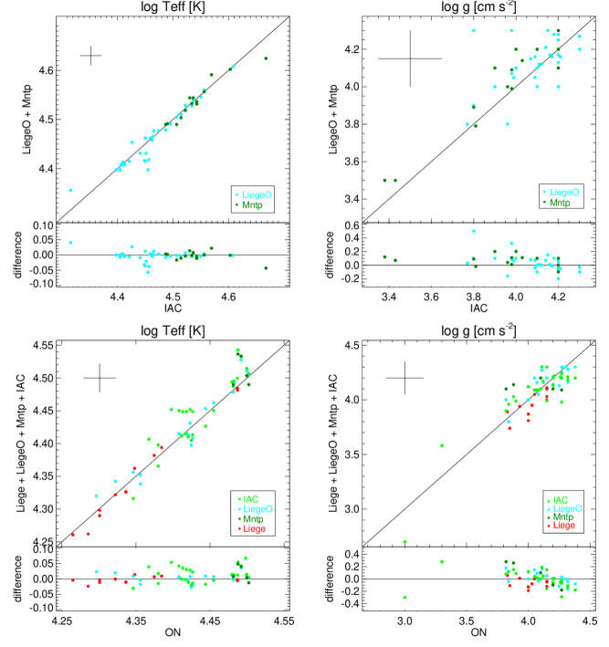
The data analysed here allow a comparison between the non-LTE codes FASTWIND and CMFGEN, which are used to determine the parameters of the hottest stars. This comparison has already been done by Massey et al. (2013) for ten LMC and SMC stars. The GES data add a further 38 Galactic stars to this. We note however that our sample has a higher metallicity, and is dominated by main-sequence stars, while the Massey et al. sample contains many supergiants. Also Holgado et al. (2018) compared their FASTWIND results to the literature values based on CMFGEN. The top panels of Fig. 7 show the results of the comparison. The effective temperature determination differs by an average of K and a median of K (in the sense CMFGEN minus FASTWIND). This difference is much lower than the typical uncertainty of the relevant Nodes, which shows a good level of precision of the different methods used. Our numbers are higher than the Massey et al. results (they find K average, K median in our sense of the difference), but are still within their estimated K fitting precision. Our standard deviation is K, the same as the Massey et al. result. Our results are even more in line with the Holgado et al. values (who find K average).
For the surface gravity we find quite different results. The difference is dex on average ( median) with a standard deviation of . This is less significant than the average and median found by Massey et al. Their standard deviation is lower, with a value of . It is not clear whether the differences between their results and ours should be attributed to the different samples (LMC/SMC vs Galactic) or to improvements in either of the codes. Again, our results are in better agreement with Holgado et al., who find dex on average.
A similar comparison can be made between the ON Node and the other Nodes that have sources in common. The bottom panels of Fig. 7 show the results; the ROBGrid Node was not included in this comparison as it was discussed previously. The differences in effective temperature (in the sense other Nodes minus ON Node) are K in average ( K in median), with a standard deviation of K. The figure also shows an increasing trend of the difference with increasing temperature.
The surface gravity is in good agreement: difference in average, in median, with a standard deviation of . Nevertheless, the difference plot again shows a linear trend, with the difference decreasing with higher values.
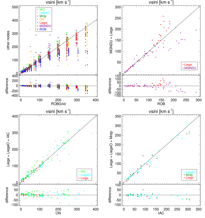
Many of the Nodes also determine . Some of the Nodes (IAC, LiègeO, and Mntp) also separate out the effect of macroturbulence. This effect can be quite important for the hottest stars, where the macroturbulence can go over 100 km s-1 in a good fraction of them (Simón-Díaz & Herrero 2014). The value of Nodes that do not derive a separate macroturbulent velocity will therefore also include the effect of some macroturbulent broadening (though it may be small in the case of the cooler stars). To allow a comparison of the results between all Nodes, we add the macroturbulent velocity (when determined) in quadrature to . This procedure may be less reliable for stars with a high , as it becomes difficult to determine a good value for the macroturbulence, but we expect that only very few stars will be affected by this. For ease of reference we refer to this total line broadening velocity hereafter as .
A comparison between the Nodes that determine is given in Fig. 8. The ROBGrid Node works with a set of discretised values to determine the . In the top left plot of Fig. 8 these values are compared to the results of the other Nodes. While there is an acceptable agreement for smaller values of , the conclusion is less clear for the larger values. Most Nodes still give an acceptable agreement for part of the data, but for another part of the data they obtain much lower values. The ROB Node even consistently finds lower values than the ROBGrid one. For the hottest stars the agreement (with the IAC, LiègeO, and Mntp Nodes) is good, even up to higher values.
We next compare those Nodes covering the lower temperature range, by plotting the MGNDU and Liège results against the ROB results (top right plot of Fig. 8). The agreement is very good at lower values, but the results deviate at the higher values: Liège finds higher values, and MGNDU finds lower values than ROB.
The bottom panels of Fig. 8 compare the middle and upper temperature ranges. In both cases there is good agreement among all the Nodes.
4.3 Recommended values
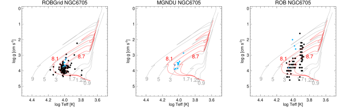
The analysis of the hot-star spectra in WG13 follows the same principles as in the case of the cool-star spectra: a homogenisation procedure is applied to the Node results, giving a single set of parameters and abundances for each star (the recommended values). Based on the results from Sect. 4.2, the ROBGrid and metallicity values were corrected for an offset before entering the homogenisation phase.
The homogenisation is based on a weighted average of the various Nodes. Ideally, this weighting scheme would be based on how well the Nodes can reproduce the results of the benchmark stars. In WG13, however, the coverage of the benchmark stars by the different Nodes is not very uniform due to the large temperature range that has to be handled for the hotter stars. We therefore use a different procedure to assign the Node weights; they are determined by how well a given Node leads to cluster results that can be fitted with a single isochrone. For each cluster that was analysed by at least two Nodes, two of us (RB and AL) made an independent by-eye judgement of which Node best fits a single isochrone161616This was done on results from iDR5.. An example of the figures in which this judgement is made is shown in Fig. 9. Nodes are judged pair-wise and two points are given to the better Node and zero to the worse one, or one point each if the difference between the two Nodes is negligible. In the specific case shown in Fig. 9, two points each are assigned to MGNDU and ROBGrid in their comparison with ROB, and one point each in the comparison between them. Weights are then assigned to each of the Nodes by adding up the points each Node received and dividing it by the number of pair-wise comparisons in which they played a role. The resulting weights are listed in Table 10.
| Node | Weight | Node | Weight | Node | Weight |
|---|---|---|---|---|---|
| ROBGrid | 0.80 | Liège | 1.50 | Mntp | 1.00 |
| ROB | 0.81 | ON | 0.58 | LiègeO | 1.50 |
| MGNDU | 1.19 | IAC | 1.50 |
The weights thus derived are applied to the homogenisation of , 171717Notwithstanding the problems discussed in Sect. 4.2, all available values were used in the homogenisation., metallicity, microturbulence, and radial velocity. For the metallicity we combine [M/H] data (where given) with [Fe/H] data (where given). For the same weights are used, except that the ROBGrid results are assigned a weight 0 as the comparison in Fig. 8 shows its results to be of lesser quality; however, if no other Node results exist, the ROBGrid value is chosen.
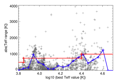
The stellar parameters are also assigned uncertainties. We attribute a fixed uncertainty for a certain range in parameter space. As an example, we show the procedure for in Fig. 10. The plus signs indicate the range of values (from the different Nodes and different GIRAFFE and UVES setups) plotted as a function of log . The log range is divided into 20 bins, and in each bin the value that contains 68.3 % of the points is determined (68.3 % corresponds to 1 for a Gaussian distribution). The blue line connects these 68.3 % points. This line is then rectified (by eye), taking into account that the uncertainty should increase with ; the rectified line is shown in red. All values within a certain range are then assigned the same uncertainty (read off from the red line). A similar approach is used for .
For metallicity and microturbulence similar figures were made, but they contain too few points to be useful. For the uncertainties on metallicity and microturbulence, we therefore take the (weighted) standard deviation of the differences between the Node results and the homogenised result. For , a similar figure was made, but it is dominated by ROBGrid results, which is not the best procedure to determine (Sect. 4.2). It was therefore decided instead to attribute a 15 % 1 uncertainty to . For results that are due to ROBGrid only, this uncertainty is in many cases smaller than the stepsize in the grid it used.
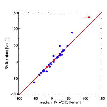
As a quality check on the radial velocities, we compare the median radial velocities of the clusters to the cluster radial velocities listed in Jackson et al. (2022). Stars flagged as binaries or radial velocity variables have not been included in the median calculation. The comparison in Fig. 11 shows that the clusters Berkeley 25, Berkeley 81, and Haffner 10 are significantly different, but the other clusters agree well (with the WG13 values on average being 2 km s-1 lower than the literature ones).
All of the Nodes have set flags for the spectra that have problems with the data reduction, or with spectral analysis. Flags are also set to describe interesting features of the spectrum (e.g. binarity). In the homogenisation phase, each star is assigned a list of flags, concatenated from the flags set for that star by the different Nodes. Discordant values between different Nodes are not flagged, however.
5 Abundances
| Cluster | He Ia𝑎aa𝑎aHe II was also used for the hottest stars, | C I | C II | C III | N II | N III | O I | O II | Ne I | Mg I | Mg II | Al II | Si II | Si III | Si IV | Sc II | |
| NGC 2516 | … | 11 | … | … | … | … | 11 | … | … | 11 | … | 11 | … | … | … | 11 | ROB |
| NGC 2547 | … | 10 | … | … | … | … | 10 | … | … | 10 | … | 10 | … | … | … | 10 | ROB |
| NGC 3293b𝑏bb𝑏barchive data. | 63 | … | 19 | … | 17 | … | … | … | 5 | … | 63 | … | … | 19 | … | … | Liège |
| NGC 3293 | 116 | … | 15 | … | 24 | … | … | … | 11 | … | 116 | … | 6 | 26 | … | … | Liège |
| NGC 6633 | … | 17 | … | … | … | … | 17 | … | … | 17 | … | 17 | … | … | … | 17 | ROB |
| NGC 6705 | … | 3 | … | … | … | … | 3 | … | … | 3 | … | 3 | … | … | … | 3 | ROB |
| Carina Neb. | … | … | … | 18 | … | … | … | 45 | … | … | … | … | 8 | 43 | 18 | … | ON |
| Carina Neb. | 59 | … | … | … | … | … | … | … | … | … | … | … | … | … | … | … | IAC |
| Carina Neb. | 66 | … | 52 | 16 | 50 | 14 | … | … | … | … | … | … | … | … | … | … | LiègeO |
Table 11 gives an overview of the number of stars for which abundances are derived for each ionic species of the elements considered here. It also lists the cluster and the Node that derived these values. Only a limited number of spectra are used to determine the abundances. One of the reasons for this is that the ROBGrid Node, which determined most of the stellar parameters, does not have the possibility to determine abundances, as explained in Sect. 3.2.1. In the lower temperature range covered by WG13, the ROB Node determines abundances only for the highest S/N spectra, while the MGNDU Node does not determine abundances. In the mid-temperature range, the Liège Node delivers values for the highest S/N spectra and the ON Node for almost all the spectra they processed. At the highest temperatures, abundances are derived for almost all stars, but the small number of stars and of spectral lines means this is limited to just a few ions of a few stars.
In GES it is standard procedure to determine these abundances with the recommended values of the stellar parameters. For hot stars, however, the use of recommended parameters that are too different from the Node values leads to clearly incorrect abundances. In the WG13 work the Node stellar parameters are therefore used to determine abundances.
The number of stars for which abundances are determined is relatively small, and there is little overlap between the different Nodes. A detailed comparison between the results is therefore not possible.
To determine the recommended values of the abundances, a non-weighted average of each abundance determination is taken. The 1 uncertainty is determined by the root mean square average. As noted above, there is very little overlap between the different Nodes, hence the recommended result for any star is usually the result of only a single Node. To give an overview of the quantity of abundance data, we show in Fig. 12 the histograms of our abundance determinations of all elements considered.
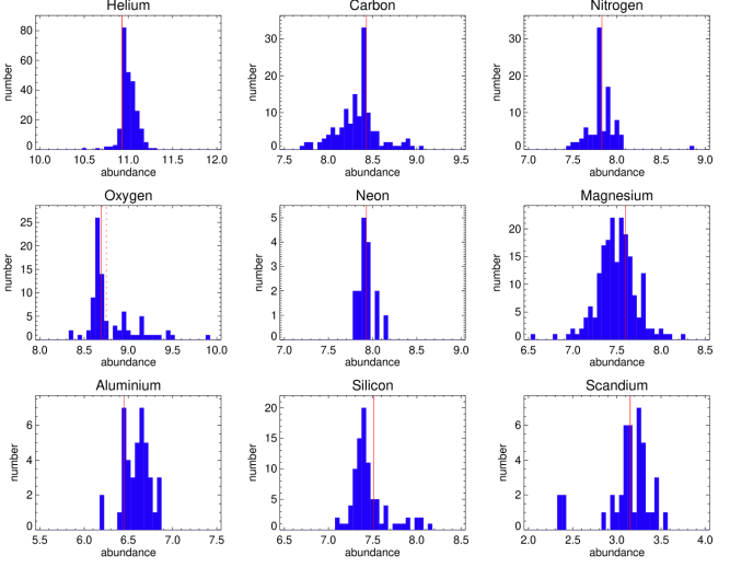
6 Summary and conclusions
In this paper we described the analysis of the hot-star spectra that were obtained by the Gaia-ESO Survey, GES. The determination of the stellar parameters and abundances followed a similar procedure to that for the cooler stars in the GES (Smiljanic et al. 2014; Lanzafame et al. 2015; Worley et al. 2022). A number of Nodes independently analysed a subset of the spectra, and the resulting parameters and abundances were then homogenised to deliver a set of recommended values. The large effective temperature range covered by these spectra required the use of different codes; most Nodes could therefore only cover part of the data. For consistency, we also determined Node abundances from the Node stellar parameters (rather than from the recommended ones, as done for the cooler stars in the GES).
We used the spectra from the last internal data release (iDR6). Quality checks on the stellar parameters were carried out by intercomparing the Node results, and by cross-checking with benchmark stars. The benchmark comparison led to some adjustments of the results of one of the Nodes (ROBGrid). The homogenisation procedure for stellar parameters consists of taking, for each star, a weighted average of the Node results, where the weights are determined by how well a single isochrone fits the Node results of each cluster.
As this is mainly a technical paper, only a few results were presented for this rich data set. The hottest stars were used for a comparison between the FASTWIND and CMFGEN codes, leading to a much larger comparison sample than was hitherto available in the literature. As for the GES data in general, the hot-star data analysed here will be of considerable use in future studies of stellar evolution and open clusters.
Acknowledgements.
This paper is based on data products from observations made with ESO Telescopes at the La Silla Paranal Observatory under programmes ID 188.B-3002, 193.B-0936, and 197.B-1074. These data products have been processed by the Cambridge Astronomy Survey Unit (CASU) at the Institute of Astronomy, University of Cambridge, and by the FLAMES/UVES reduction team at INAF/Osservatorio Astrofisico di Arcetri. This work was partly supported by the European Union FP7 programme through ERC grant number 320360 and by the Leverhulme Trust through grant RPG-2012-541. We acknowledge the support from INAF and Ministero dell’ Istruzione, dell’ Università’ e della Ricerca (MIUR) in the form of the grant ‘Premiale VLT 2012’. The results presented here benefitted from discussions held during the Gaia-ESO workshops and conferences supported by the ESF (European Science Foundation) through the GREAT Research Network Programme. We are grateful to E. Bertone for making their high-resolution models available, as well as to R. Sordo for making the high-resolution Munari models available. This research has made use of the WEBDA database, originally developed by Jean-Claude Mermilliod, and now operated at the Department of Theoretical Physics and Astrophysics of the Masaryk University. This research has also made use of the SIMBAD database, operated at CDS, Strasbourg, France. A.H. acknowledges support by the Spanish Ministerio de Ciencia e Innovación through grants PGC2018-091 3741-B-C22 and CEX-2019-000920-S. The work of S.R.B, I.N., and S.S.D. is partially supported by the Spanish Government Ministerio de Economía y Competitivad (MINECO/FEDER) under grants PGC2018-093741-B-C21/C22 (MICIU/AEI/FEDER, UE). A.L. acknowledges that his research has been funded in part by the Belgian Federal Science Policy Office under contract No. BR/143/A2/BRASS. The Liège Node is grateful to Belgian F.R.S.-FNRS for various supports. They are also indebted for an ESA/PRODEX Belspo contract related to the Gaia Data Processing and Analysis Consortium and for support through an ARC grant for Concerted Research Actions financed by the Federation Wallonie-Brussels. J.M.A. acknowledges support from the Spanish Government Ministerio de Ciencia through grants AYA2016-75 931-C2-2-P and PGC2018-095 049-B-C22. W.S. acknowledges CAPES for a Ph.D. Fellowship. G.H. acknowledges that this research has been partially funded by the Canarian Agency for Economy, Knowledge, and Employment and the European Regional Development Fund (ERDF/EU), under grant with reference ProID2020010016. F.J.E. acknowledges financial support from the Spanish MINECO/FEDER through the grant AYA2017-84089 and MDM-2017-0737 at Centro de Astrobiología (CSIC-INTA), Unidad de Excelencia María de Maeztu, and from the European Union’s Horizon 2020 research and innovation programme under Grant Agreement no. 824064 through the ESCAPE - The European Science Cluster of Astronomy & Particle Physics ESFRI Research Infrastructures project. E.J.A acknowledges funding from the State Agency for Research of the Spanish MCIU through the ‘Center of Excellence Severo Ochoa’ award to the Instituto de Astrofísica de Andalucía (SEV-2017-0709) and from MCIU grant PGC2018-095049-B-C21. T.B. acknowledges financial support by grant No. 2018-04857 from the Swedish Research Council. A.J.K. and U.H. acknowledge support from the Swedish National Space Agency (SNSA). R.S. acknowledges support from the National Science Centre (2014/15/B/ST9/03981).References
- Asplund et al. (2009) Asplund, M., Grevesse, N., Sauval, A. J., & Scott, P. 2009, ARA&A, 47, 481
- Bell et al. (2013) Bell, C. P. M., Naylor, T., Mayne, N. J., Jeffries, R. D., & Littlefair, S. P. 2013, MNRAS, 434, 806
- Bergemann et al. (2021) Bergemann, M., Hoppe, R., Semenova, E., et al. 2021, MNRAS, 508, 2236
- Berlanas et al. (2018) Berlanas, S. R., Herrero, A., Comerón, F., et al. 2018, A&A, 620, A56
- Berlanas et al. (2020) Berlanas, S. R., Herrero, A., Comerón, F., et al. 2020, A&A, 642, A168
- Bertone et al. (2008) Bertone, E., Buzzoni, A., Chávez, M., & Rodríguez-Merino, L. H. 2008, A&A, 485, 823
- Bonifacio et al. (2012) Bonifacio, P., Caffau, E., Ludwig, H.-G., & Steffen, M. 2012, in IAU Symposium, Vol. 282, From Interacting Binaries to Exoplanets: Essential Modeling Tools, ed. M. T. Richards & I. Hubeny, 213–220
- Bragaglia et al. (2021) Bragaglia, A., Alfaro, E., Flaccomio, E., et al. 2021, arXiv e-prints, arXiv:2112.11974
- Bragança et al. (2019) Bragança, G. A., Daflon, S., Lanz, T., et al. 2019, A&A, 625, A120
- Burkhart & Coupry (1989) Burkhart, C. & Coupry, M. F. 1989, A&A, 220, 197
- Butler (1984) Butler, K. 1984, PhD thesis, University of London, UK
- Cantat-Gaudin et al. (2020) Cantat-Gaudin, T., Anders, F., Castro-Ginard, A., et al. 2020, A&A, 640, A1
- Castelli & Kurucz (2003) Castelli, F. & Kurucz, R. L. 2003, in IAU Symposium, Vol. 210, Modelling of Stellar Atmospheres, ed. N. Piskunov, W. W. Weiss, & D. F. Gray, A20
- Coelho et al. (2005) Coelho, P., Barbuy, B., Meléndez, J., Schiavon, R. P., & Castilho, B. V. 2005, A&A, 443, 735
- Conrad et al. (2017) Conrad, C., Scholz, R. D., Kharchenko, N. V., et al. 2017, A&A, 600, A106
- Crowther et al. (2006) Crowther, P. A., Lennon, D. J., & Walborn, N. R. 2006, A&A, 446, 279
- Daflon et al. (2007) Daflon, S., Cunha, K., de Araújo, F. X., Wolff, S., & Przybilla, N. 2007, AJ, 134, 1570
- David et al. (2014) David, M., Blomme, R., Frémat, Y., et al. 2014, A&A, 562, A97
- de Jager et al. (1997) de Jager, C., Lobel, A., & Israelian, G. 1997, A&A, 325, 714
- Ekström et al. (2012) Ekström, S., Georgy, C., Eggenberger, P., et al. 2012, A&A, 537, A146
- Evans et al. (2005) Evans, C. J., Smartt, S. J., Lee, J.-K., et al. 2005, A&A, 437, 467
- Gazzano et al. (2010) Gazzano, J.-C., de Laverny, P., Deleuil, M., et al. 2010, A&A, 523, A91
- Gebran et al. (2016) Gebran, M., Farah, W., Paletou, F., Monier, R., & Watson, V. 2016, A&A, 589, A83
- Gebran et al. (2014) Gebran, M., Monier, R., Royer, F., Lobel, A., & Blomme, R. 2014, in Putting A Stars into Context: Evolution, Environment, and Related Stars, ed. G. Mathys, E. R. Griffin, O. Kochukhov, R. Monier, & G. M. Wahlgren, 193–198
- Gilmore et al. (2012) Gilmore, G., Randich, S., Asplund, M., et al. 2012, The Messenger, 147, 25
- Gilmore et al. (2022) Gilmore, G., Randich, S., Worley, C. C., et al. 2022, A&A, submitted
- Girard et al. (2011) Girard, T. M., van Altena, W. F., Zacharias, N., et al. 2011, AJ, 142, 15
- Gray (2005) Gray, D. F. 2005, The Observation and Analysis of Stellar Photospheres, 3rd edn. (Cambridge University Press)
- Gray et al. (2001) Gray, R. O., Graham, P. W., & Hoyt, S. R. 2001, AJ, 121, 2159
- Grevesse et al. (2007) Grevesse, N., Asplund, M., & Sauval, A. J. 2007, Space Sci. Rev., 130, 105
- Heiter et al. (2015) Heiter, U., Jofré, P., Gustafsson, B., et al. 2015, A&A, 582, A49
- Hillier & Miller (1998) Hillier, D. J. & Miller, D. L. 1998, ApJ, 496, 407
- Holgado et al. (2018) Holgado, G., Simón-Díaz, S., Barbá, R. H., et al. 2018, A&A, 613, A65
- Holgado et al. (2020) Holgado, G., Simón-Díaz, S., Haemmerlé, L., et al. 2020, A&A, 638, A157
- Hourihane et al. (2022) Hourihane, A., XXX, X., & XXX, X. 2022, A&A, in preparation
- Hubeny & Lanz (1992) Hubeny, I. & Lanz, T. 1992, A&A, 262, 501
- Hubeny & Lanz (1995) Hubeny, I. & Lanz, T. 1995, ApJ, 439, 875
- Hubeny & Lanz (2017) Hubeny, I. & Lanz, T. 2017, ArXiv e-prints [arXiv:1706.01859]
- Hubrig et al. (2008) Hubrig, S., Briquet, M., Morel, T., et al. 2008, A&A, 488, 287
- Jackson et al. (2015) Jackson, R. J., Jeffries, R. D., Lewis, J., et al. 2015, A&A, 580, A75
- Jackson et al. (2022) Jackson, R. J., Jeffries, R. D., Wright, N. J., et al. 2022, MNRAS, 509, 1664
- Jofré et al. (2014) Jofré, P., Heiter, U., Soubiran, C., et al. 2014, A&A, 564, A133
- Jofré et al. (2018) Jofré, P., Heiter, U., Tucci Maia, M., et al. 2018, Research Notes of the American Astronomical Society, 2, 152
- Kassounian et al. (2019) Kassounian, S., Gebran, M., Paletou, F., & Watson, V. 2019, Open Astronomy, 28, 68
- Kaufer et al. (2011) Kaufer, A., Martayan, C., & Melo, C. 2011, Very Large Telescope Paranal Science Operations FLAMES User Manual, ESO
- Kurucz (1992) Kurucz, R. L. 1992, Rev. Mexicana Astron. Astrofis., 23
- Kurucz (1993) Kurucz, R. L. 1993, in Astronomical Society of the Pacific Conference Series, Vol. 44, IAU Colloq. 138: Peculiar versus Normal Phenomena in A-type and Related Stars, ed. M. M. Dworetsky, F. Castelli, & R. Faraggiana, 87
- Lanz & Hubeny (2003) Lanz, T. & Hubeny, I. 2003, ApJS, 146, 417
- Lanz & Hubeny (2007) Lanz, T. & Hubeny, I. 2007, ApJS, 169, 83
- Lanzafame et al. (2015) Lanzafame, A. C., Frasca, A., Damiani, F., et al. 2015, A&A, 576, A80
- Laverick et al. (2019) Laverick, M., Lobel, A., Royer, P., et al. 2019, A&A, 624, A60
- Lefever et al. (2010) Lefever, K., Puls, J., Morel, T., et al. 2010, A&A, 515, A74
- Lobel (2008) Lobel, A. 2008, in Journal of Physics Conference Series, Vol. 130, Journal of Physics Conference Series, 012015
- Lobel (2011a) Lobel, A. 2011a, Canadian Journal of Physics, 89, 395
- Lobel (2011b) Lobel, A. 2011b, in Journal of Physics Conference Series, Vol. 328, Journal of Physics Conference Series, 012027
- Lobel et al. (2017) Lobel, A., Royer, P., Martayan, C., et al. 2017, Canadian Journal of Physics, 95, 833
- Mahy et al. (2020) Mahy, L., Sana, H., Abdul-Masih, M., et al. 2020, A&A, 634, A118
- Maíz Apellániz et al. (2018) Maíz Apellániz, J., Pantaleoni González, M., Barbá, R. H., et al. 2018, A&A, 616, A149
- Martins et al. (2012) Martins, F., Escolano, C., Wade, G. A., et al. 2012, A&A, 538, A29
- Martins et al. (2015) Martins, F., Hervé, A., Bouret, J.-C., et al. 2015, A&A, 575, A34
- Martins et al. (2005) Martins, F., Schaerer, D., & Hillier, D. J. 2005, A&A, 436, 1049
- Massey et al. (2013) Massey, P., Neugent, K. F., Hillier, D. J., & Puls, J. 2013, ApJ, 768, 6
- Merle et al. (2017) Merle, T., Van Eck, S., Jorissen, A., et al. 2017, A&A, 608, A95
- Mokiem et al. (2005) Mokiem, M. R., de Koter, A., Puls, J., et al. 2005, A&A, 441, 711
- Morel & Butler (2008) Morel, T. & Butler, K. 2008, A&A, 487, 307
- Morel et al. (2006) Morel, T., Butler, K., Aerts, C., Neiner, C., & Briquet, M. 2006, A&A, 457, 651
- Munari et al. (2005) Munari, U., Sordo, R., Castelli, F., & Zwitter, T. 2005, A&A, 442, 1127
- Netopil et al. (2016) Netopil, M., Paunzen, E., Heiter, U., & Soubiran, C. 2016, A&A, 585, A150
- Nieva & Przybilla (2008) Nieva, M. F. & Przybilla, N. 2008, A&A, 481, 199
- Nieva & Przybilla (2012) Nieva, M. F. & Przybilla, N. 2012, A&A, 539, A143
- Nieva & Simón-Díaz (2011) Nieva, M.-F. & Simón-Díaz, S. 2011, A&A, 532, A2
- Palacios et al. (2010) Palacios, A., Gebran, M., Josselin, E., et al. 2010, A&A, 516, A13
- Paletou et al. (2015) Paletou, F., Gebran, M., Houdebine, E. R., & Watson, V. 2015, A&A, 580, A78
- Pancino et al. (2017) Pancino, E., Lardo, C., Altavilla, G., et al. 2017, A&A, 598, A5
- Pasquini et al. (2002) Pasquini, L., Avila, G., Blecha, A., et al. 2002, The Messenger, 110, 1
- Press et al. (2007) Press, W., Teukolsky, S., Vetterling, W., & Flannery, B. 2007, Numerical Recipes: The Art of Scientific Computing, 3rd edn. (Cambridge University Press)
- Prugniel et al. (2011) Prugniel, P., Vauglin, I., & Koleva, M. 2011, A&A, 531, A165
- Puls et al. (1996) Puls, J., Kudritzki, R. P., Herrero, A., et al. 1996, A&A, 305, 171
- Puls et al. (2005) Puls, J., Urbaneja, M. A., Venero, R., et al. 2005, A&A, 435, 669
- Ramírez-Agudelo et al. (2013) Ramírez-Agudelo, O. H., Simón-Díaz, S., Sana, H., et al. 2013, A&A, 560, A29
- Randich et al. (2013) Randich, S., Gilmore, G., & Gaia-ESO Consortium. 2013, The Messenger, 154, 47
- Randich et al. (2022) Randich, S., Gilmore, G., Magrini, L., et al. 2022, A&A, submitted
- Sacco et al. (2014) Sacco, G. G., Morbidelli, L., Franciosini, E., et al. 2014, A&A, 565, A113
- Santolaya-Rey et al. (1997) Santolaya-Rey, A. E., Puls, J., & Herrero, A. 1997, A&A, 323, 488
- Sbordone et al. (2004) Sbordone, L., Bonifacio, P., Castelli, F., & Kurucz, R. L. 2004, Memorie della Societa Astronomica Italiana Supplementi, 5, 93
- Searle et al. (2008) Searle, S. C., Prinja, R. K., Massa, D., & Ryans, R. 2008, A&A, 481, 777
- Simón-Díaz (2010) Simón-Díaz, S. 2010, A&A, 510, A22
- Simón-Díaz et al. (2011) Simón-Díaz, S., Castro, N., Herrero, A., et al. 2011, in Journal of Physics Conference Series, Vol. 328, Journal of Physics Conference Series, 012021
- Simón-Díaz et al. (2017) Simón-Díaz, S., Godart, M., Castro, N., et al. 2017, A&A, 597, A22
- Simón-Díaz & Herrero (2007) Simón-Díaz, S. & Herrero, A. 2007, A&A, 468, 1063
- Simón-Díaz & Herrero (2014) Simón-Díaz, S. & Herrero, A. 2014, A&A, 562, A135
- Simón-Díaz et al. (2006) Simón-Díaz, S., Herrero, A., Esteban, C., & Najarro, F. 2006, A&A, 448, 351
- Smalley (2004) Smalley, B. 2004, in IAU Symposium, Vol. 224, The A-Star Puzzle, ed. J. Zverko, J. Ziznovsky, S. J. Adelman, & W. W. Weiss, 131–138
- Smiljanic et al. (2014) Smiljanic, R., Korn, A. J., Bergemann, M., et al. 2014, A&A, 570, A122
- Smith & Dworetsky (1993) Smith, K. C. & Dworetsky, M. M. 1993, A&A, 274, 335
- Sota et al. (2014) Sota, A., Maíz Apellániz, J., Morrell, N. I., et al. 2014, ApJS, 211, 10
- Sota et al. (2011) Sota, A., Maíz Apellániz, J., Walborn, N. R., et al. 2011, ApJS, 193, 24
- Thompson et al. (2008) Thompson, H. M. A., Keenan, F. P., Dufton, P. L., et al. 2008, MNRAS, 383, 729
- Vink et al. (2000) Vink, J. S., de Koter, A., & Lamers, H. J. G. L. M. 2000, A&A, 362, 295
- Vink et al. (2001) Vink, J. S., de Koter, A., & Lamers, H. J. G. L. M. 2001, A&A, 369, 574
- Walborn et al. (2002) Walborn, N. R., Danks, A. C., Vieira, G., & Landsman, W. B. 2002, ApJS, 140, 407
- Worley et al. (2022) Worley, C., XXX, X., & XXX, X. 2022, A&A, in preparation
- Zacharias et al. (2013) Zacharias, N., Finch, C. T., Girard, T. M., et al. 2013, AJ, 145, 44
Appendix A Supplementary material
To show the range and diversity of the spectra analysed by WG13, as well as the different techniques applied by the different Nodes, we present some typical examples. Figure 13 shows a number of GIRAFFE spectra and their analysis (fits) by some of the Nodes. The Mntp and ON Nodes provide a full-spectrum analysis. This is also done by the IAC Node, but a number of spectral lines are not included in their code. The Liège Node does a full-spectrum analysis and also fits in detail a number of spectral lines for abundance determination.
Figure 14 shows two examples of UVES data. The MGNDU Node (top panel) uses information from the full spectrum to determine the stellar parameters. The ROB Node (bottom panel) fits a number of spectral lines to determine both stellar parameters and abundances.
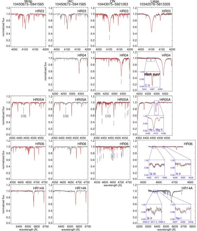
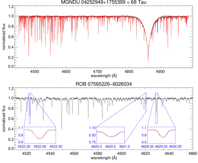
In Table 12 we show the comparison of the Node (other than ROBGrid) stellar parameters to the benchmark values.
| Benchmark | Benchmark | ROB | MGNDU | Liège | ON | IAC | Mntp | |
|---|---|---|---|---|---|---|---|---|
| star | parameters | Node | Node | Node | Node | Node | Node | |
| Procyon | K | .. | … | … | … | … | ||
| .. | … | … | … | … | ||||
| [Fe/H] = 0.01 | .. | … | … | … | … | |||
| 68 Tau | K | .. | .. | … | … | … | … | |
| .. | … | … | … | … | ||||
| [Fe/H] = 0.13 | … | … | … | … | ||||
| 134 Tau | K | .. | .. | .. | … | … | … | |
| .. | .. | .. | … | … | … | |||
| [Fe/H] = -0.05 | .. | … | … | … | … | |||
| HD 56613 | K | … | … | .. | … | … | … | |
| … | … | .. | … | … | … | |||
| 67 Oph | K | … | … | … | … | … | ||
| … | … | … | … | … | ||||
| HD 35912 | K | … | … | .. | … | … | ||
| … | … | .. | … | … | ||||
| Peg | K | … | … | .. | … | … | ||
| … | … | .. | … | … | ||||
| V900 Sco | K | … | … | … | … | … | ||
| … | … | … | … | … | ||||
| HD 68450 | K | … | … | … | ||||
| … | … | … | ||||||
| Car | K | … | … | … | … | |||
| … | … | … | … | |||||
| Sco | K | … | … | .. | … | |||
| … | … | .. | … | |||||
| HD 163758 | K | … | … | … | … | |||
| … | … | … | … | |||||
| HD 46202 | K | … | … | … | … | |||
| … | … | … | … | |||||
| HDE 319699 | K | … | … | … | … | … | ||
| … | … | … | … | … |