Photon frequency diffusion process

Abstract

We introduce a stochastic multi-photon dynamics on reciprocal space. Assuming isotropy, we derive the diffusion limit for a tagged photon to be a nonlinear Markov process on frequency. The nonlinearity stems from the stimulated emission. In the case of Compton scattering with thermal electrons, the limiting process describes the dynamical fluctuations around the Kompaneets equation. More generally, we construct a photon frequency diffusion process which enables to include nonequilibrium effects. Modifications of the Planck Law may thus be explored, where we focus on the low-frequency regime.

I Introduction

Time-dependent and nonequilibrium dynamics of photons are of increasing interest in a wide range of subjects. Quantum electromagnetic fields can be manipulated to produce photonic lattices (spatial network of coupled photon modes) where time-dependent driving leads to a breaking of time-reversal invariance (synthetic magnetic field) koch ; fang ; roushan . Same thing for wave guides where the input field may be driven by either a laser or microwave generator, imposing a nonequilibrium boundary condition on the propagating photons pozar ; roy . In quantum optomechanical studies photon gases may be enclosed in cavities with time-dependent geometry such as from vibrating walls, metaphotonics . In another domain and since much longer, plasma physics has dealt with the problem of understanding the origin of suprathermal tails supra1 ; banerjee and high-energy cosmic radiation as a result of the scattering of electrons with turbulent electromagnetic fields fermi ; sturrock ; brin . Finally, in Early Universe cosmology, the dynamical origin of the main features of the cosmic background radiation (CMB) remains of central importance, especially to understand (possible) deviations from homogeneity dark or from the Planck Law arcade1 ; arcade2 ; edges ; arca .
As understood from the pioneering days of statistical mechanics and in analogy with Brownian motion, we may expect that the studies mentioned above benefit from modeling fluctuations, i.e., to identify the random motion in photon frequency space. For example, considering a mesoscopic level of description, we become able to insert nonequilibrium effects on the single-photon level allowing to discover meaningful modifications of the Planck Law.

In the present paper we derive a (stochastic) diffusion process for a tagged photon, that can be seen as the diffusion limit of a multi-photon hopping dynamics in reciprocal space. Stimulated emission results in the nonlinearity of the Markov diffusion process.
We first apply our construction to build a Kompaneets process, i.e., the stochastic (single-photon) dynamics that has the well-known Kompaneets equation as its nonlinear Fokker-Planck equation. That new fluctuation dynamics is the counterpart to the analysis of Kompaneets in kompa and makes our first main result: the derivation of the frequency diffusion process for a tagged photon in a plasma dominated by Compton scattering. Similarly, many other processes such as double Compton and Bremsstrahlung can be considered, and thanks to our setup, are easily added to the dynamics, turning it into a fully nonlinear reaction-diffision dynamics. Not only does that process complement (in some precise sense) the Kompaneets equation, it allows also to see beyond, leading to our second main contribution. A possible avenue indeed that gets opened, is the implementation and exploration of nonequilibrium effects modifying the Planck law, via physically motivated interventions on the single-photon level. Our work explores how changing drift and adding diffusion may change the low-frequency distribution, where the relaxation times in the Kompaneets process are largest, hence most vulnerable to nonequilibrium amendments.
As a final remark, it should be noted in all these cases that we start from a multi-photon diffusion process in frequency space. It means to include the stimulated emission in the reactivities. That presents a nontrivial aspect in both the theoretical and computational analysis, leading finally to important nonlinearities in the corresponding Fokker-Planck equation. However, our results indicate that the processes simulate indeed the Kompaneets equation and its extensions, in the sense that the empirical density of photons follows these equations.

In the next section we describe the Kompaneets equation for relaxation to the Planck law via Compton scattering. In Section III we introduce the Kompaneets process, describing the hopping of photons in reciprocal space. Its diffusion limit for a tagged photon gives a nonlinear Markov process, described in Eq. (21). That simulation is explained in Section IV, where the results are shown in terms of the time-dependence of the spectral density. We confirm the validity of the simulation scheme by verifying relaxation to the Planck law along the Kompaneets equation. There, we also show the appearance of a condensate when the number of photons is taken to be large enough, an effect already observed in levermore . Other non photon-number preserving radiation processes are added in Section V. Bremsstrahlung and double Compton scattering are described there as low-frequency corrections. These are reactive mechanisms to control photon-number that can be handled and taken effectively in the simulation. Section VI discusses more general photon-number processes, extending the Kompaneets process to implement two types of low-frequency modifications, either in the drift or in the diffusion. They are nonequilibrium features in the photon dynamics, effectively implementable on the single-photon level that we simulate. Finally, in Section VII, we explain the simulation details for that extension (including reactive mechanisms). That illustrates in great detail how nonequilibrium features change the stationary solution to enhance low-frequency occupation (yielding there a higher effective temperature).

II Kompaneets equation

The Compton effect is a quantum process in which photons scatter from free electrons. It eventually leads to the relaxation of the photon distribution to that of the Planck radiation law. The Kompaneets equation

$$\omega^{2}\frac{\partial n}{\partial t}(t,\omega)=\frac{n_{e}\sigma_{T}c}{m_{e}c^{2}}\frac{\partial}{\partial\omega}\omega^{4}\left\{k_{B}T\frac{\partial n}{\partial\omega}(t,\omega)+\hbar\left[1+n(t,\omega)\right]n(t,\omega)\right\}$$ (1)

describes that relaxation towards equilibrium of a photon gas in contact with a nondegenerate, nonrelativistic electron bath in thermal equilibrium at temperature $T$. Here, $n(t,\omega)$ is the average occupation number at frequency $\omega$ of the photon gas at time $t$; stationarity is then achieved when $n(t,\omega)$ reaches the Bose-Einstein distribution. Apart from the usual constants in (1), we recognize $\sigma_{T}$ as the Thomson total cross section and $n_{e},m_{e}$ as the density and mass of the electrons, respectively. The induced Compton scattering liedahl ; blandford leads to the nonlinearity (in the second term) appearing in the Kompaneets equation (1).
In 1957 Kompaneets kompa gave a mesoscopic derivation of (1), starting from a semi-classical Boltzmann equation. It remains essential for the understanding of the CMB spectrum and related phenomena such as the Sunyaev-Zeldovich effect sunyaeveffect ; sunyaev . The understanding of the Kompaneets equation has been evolving over the years and excellent reviews include practical ; gui ; zeldovich . We emphasize that many extensions to the equation exist. For example, the isotropy condition for the distribution has been relaxed in buet ; pitrou , while nonrelativistic extensions can be found in barbosa ; brown ; itoh ; itoh2 ; cooper ; kohyama1 ; kohyama2 ; kohyama3 . More recently in paper we addressed some consistency problems in Kompaneets’ original framework kompa .

For simplicity it is convenient to use the dimensionless counterpart of (1) in order to introduce (in the next Section) the Kompaneets process, which describes the hopping of photons in reciprocal space.
The dynamics of the average photon occupation number $n(t,x)$ at dimensionless frequency $x=\hbar\omega/k_{B}T$ in a thermal environment with temperature $T$, is obtained from equation (1) as

$$x^{2}\frac{\partial n}{\partial t}(y,x)=\frac{\partial}{\partial x}x^{4}\left\{\frac{\partial n}{\partial x}(y,x)+\left[1+n(y,x)\right]n(y,x)\right\}$$ (2)

where we have defined the dimensionless Compton optical depth

$$y=\frac{k_{B}T}{m_{e}c^{2}}n_{e}\sigma_{T}c\,t=\frac{t}{\tau_{C}}.$$

Here, $\tau_{C}$ is the characteristic time in which photons change their frequency due to Compton scattering with thermal electrons,

$$\left\langle\frac{1}{2\tau}\left(\frac{\Delta\omega}{\omega}\right)^{2}\right\rangle\approx\frac{k_{B}T}{m_{e}c^{2}}\;\frac{1}{\tau}=\frac{1}{\tau_{C}}$$ (3)

where $\tau=l/c$ is the average collision rate, related to the mean free path of photons $l=(n_{e}\sigma_{T})^{-1}$. For simplicity, we will take our units such that $\tau_{C}=1$, identifing $y$ with $t$.
Note that the

$$n_{\mu}(x)=\frac{1}{e^{x-\mu}-1},\qquad\mu\leq 0$$ (4)

are stationary solutions of (2): $\frac{\differential n_{\mu}}{\differential x}(x)+[1+n_{\mu}(x)]\,n_{\mu}(x)=0$.

Central for our purposes to simulate the Compton scattering on a mesoscopic level is to write the Kompaneets equation (1)–(2) in terms of the photon density. Assuming that photons are confined to a box of volume $V$ with periodic boundary conditions, the density of states is

$$g(\mathbf{k})\differential^{3}\mathbf{k}=\frac{2V}{(2\pi)^{3}}\differential^{3}\mathbf{k}=\frac{2V}{(2\pi)^{3}}4\pi k^{2}\differential k$$

where $\mathbf{k}$ is the wave vector. It is useful here to assume isotropy: in function of the dimensionless $x=\hbar\omega/k_{B}T$, the density of states is

$$g(x)\differential x=\frac{2V}{(2\pi)^{3}}\left(\frac{k_{B}T}{\hbar c}\right)^{3}4\pi x^{2}\differential x$$

From here we can integrate the photon occupation number to get the total number of photons

$$N_{t}=\int_{0}^{\infty}\differential{x}g(x)n(t,x)$$

That allows to write the spectral probability density

$$\rho(t,x)=\frac{V}{N_{t}}\frac{1}{\pi^{2}}\left(\frac{k_{B}T}{\hbar c}\right)^{3}x^{2}n(t,x)=\frac{x^{2}n(t,x)}{2\zeta(3)Z_{t}},$$ (5)

where $2\zeta(3)=\int_{0}^{\infty}\differential x\,x^{2}/(e^{x}-1)\simeq 2.404$. By using the normalization of the spectral probability density while integrating (5) over $x$, we can write

$$Z_{t}=\frac{1}{2\zeta(3)}\,\int_{0}^{\infty}\differential x\,x^{2}n(t,x)\propto\frac{N_{t}}{V}\left(\frac{\hbar c}{k_{B}T}\right)^{3}$$ (6)

which is a possibly time-dependent parameter, depending on the temperature and proportional to the number of photons per volume. Since the Kompaneets equation (still without reaction mechanism) is photon-number preserving, $Z_{t}=Z$ is time-independent and yields for the stationary $n_{\mu}$ in (4),

$$Z=\frac{\text{Li}_{3}(e^{\mu})}{\zeta(3)}$$

with Li₃ the polylogarithm of order 3. In that notation, the Kompaneets equation (2) becomes

$$\frac{\partial\rho}{\partial t}(t,x)=-\frac{\partial}{\partial x}\left[\left(4x-x^{2}\left(1+2\zeta(3)Z\,\frac{\rho(t,x)}{x^{2}}\right)\right)\rho(t,x)\right]+\frac{\partial^{2}}{\partial x^{2}}\left[x^{2}\rho(t,x)\right]$$ (7)

Observe still that $Z$ can be interpreted as the ratio of the actual photon spectral density to that of the Planck distribution corresponding to the same temperature. For the Bose-Einstein distribution $n(t,x)=n_{\text{BE}}(x)=n_{0}(x)=1/(e^{x}-1)$, the photon number equals

$$N_{\text{BE}}=2\zeta(3)\frac{V}{\pi^{2}}\left(\frac{k_{B}T}{\hbar c}\right)^{3}$$

corresponding to a spectral probability density with $Z=1$:

$$\rho_{\text{BE}}(x)=\frac{x^{2}n_{BE}(x)}{2\zeta(3)}$$ (8)

We make a “hot” Planck spectral density by changing $x\rightarrow x/2$ (doubling the temperature), taking $n(x)=n_{\text{BE}}(x/2)$, leading to

$$\rho_{\text{BE}}^{\text{hot}}(x)=\frac{x^{2}n_{\text{BE}}(x/2)}{16\zeta(3)}$$ (9)

in which case $Z=8$. On the other hand, as $Z$ goes to zero, we recover the Wien expression $\rho_{\text{Wien}}(x)=x^{2}e^{-x}/2$ to be the stationary spectral probability density for equation (7) which becomes linear at $Z=0$.

As a final comment we note that the Kompaneets equation is positivity preserving positivity . That is important because any solution of the equation will retain its sign, suggesting indeed to interpret this equation as of Fokker-Planck type.

III Mesoscopics of Compton scattering: Kompaneets stochastic process

When considering a single Compton scattering event, the transition rates are fully determined by the incident electron and photon momenta together with energy-momentum conservation. However, in the presence of repeated scattering, treating the electron as a classical particle and the photon as a boson, the transition rates must account for stimulated emission, i.e., transitions are enhanced if photons are present in the final state. Mathematically, we work on a symmetrized Fock space kadanoff , where transition rates (between incoming $|\text{i}\rangle$ and final states $|\text{f}\rangle$) have an additional term coming from the matrix element

$$\left|\langle\text{f}\,|a^{\dagger}_{{\mathbf{k}^{\prime}}}a_{\mathbf{k}}|\text{i}\rangle\right|^{2}=(1+n({\mathbf{k}^{\prime}}))\,n({\mathbf{k}})$$ (10)

where $a^{(\dagger)}_{\mathbf{k}}$ are the annihilation (creation) operators in the Fock space related to the photon momentum $\mathbf{k}$, and $n({\mathbf{k}})$ are occupation numbers. That is the only “interaction” between the photons that we take into account so far.

III.1 Jump process in reciprocal space

As introduced in paper , we start from a random walk of bosons in reciprocal space. Here we consider a bath of a large number $N$ of photons, confined to a cube of sidelength $\ell$ with periodic boundary conditions. We will end up working in the thermodynamic limit for fixed density $N/\ell^{3}$. For now however the modes are quantized, at a fixed distance $\delta=2\pi/\ell$. We designate each photon by its wave vector $\mathbf{k}_{i}$ so that the full state of the bath is described by $\mathbf{K}=(\mathbf{k}_{1},\dots,\mathbf{k}_{N})$. Yet, we must treat the photons indistinguishably, and soon we will work with occupation numbers.
Transitions $\mathbf{K}\rightarrow\mathbf{K}^{\prime}$ between states are restricted to these for which only one photon jumps to another wave vector, i.e., to transitions

$$\mathbf{K}=(\mathbf{k}_{1},\dots,\mathbf{k}_{i},\ldots,\mathbf{k}_{N})\longrightarrow\mathbf{K}^{\prime}=(\mathbf{k}_{1},\dots,\mathbf{k}_{i}+\mathbf{a}\delta,\dots,\mathbf{k}_{N})$$

where $\mathbf{a}$ is one of the six unit vectors. The corresponding rate of such a transition is of the form

$$w_{i}(\mathbf{K},\mathbf{a}\delta)=w(\mathbf{k}_{i},\mathbf{a}\delta)\left(1+n_{\mathbf{k}_{i}+\mathbf{a}\delta}(\mathbf{K})\right)$$

where

$$n_{\mathbf{k}}(\mathbf{K})=\sum_{i}\delta_{\mathbf{k},\mathbf{k}_{i}}$$

(with the Kronecker delta) counts the number of photons at $\mathbf{k}$. It realizes the stimulated emission in the process. The rest of the rates is taken as usual,

$$w(\mathbf{k},\mathbf{a}\delta)=D\left(\mathbf{k}+\frac{\mathbf{a}\delta}{2}\right)\exp\left\{-\frac{\beta}{2}\left(U(\mathbf{k}+\mathbf{a}\delta)-U(\mathbf{k})\right)\right\}$$

to satisfy detailed balance with energy function $U$ at inverse temperature $\beta$. We also added a (time-symmetric) reactivity $D$, also to be specified below in the case of Compton scattering.

The thus defined process $\mathbf{K}(t)$ is Markovian and has backward generator $L_{\delta}$, to be applied to observables $F(\mathbf{K})$, given by

$$L_{\delta}F(\mathbf{K})=\sum_{i,\mathbf{a}}w_{i}(\mathbf{K},\mathbf{a}\delta)\left(F(\mathbf{K}^{\prime})-F(\mathbf{K})\right)$$ (11)

where $\mathbf{k}^{\prime}_{j}=\mathbf{k}_{j}$ for $j\neq i$ and $\mathbf{k}^{\prime}_{i}=\mathbf{k}_{i}+\mathbf{a}\delta$. So far, the process can be seen as a generalized zero range process blythe . That generalization is sometimes referred to as a “misanthrope process”, motivated by the convenience of monotonicity; see cocozza ; sethuraman . Here that name is less appropriate as the dependence on the target configuration is one of “stimulation”.
We are not staying with the multiparticle dynamics generated by (11), as we wish to find the dynamics for a single tagged photon. To have a rigorous understanding of the dynamics of a tagged particle in a “misanthrope” (or stimulated) zero range process is far from trivial; see also jara . Our approach will therefore be more heuristic.

To start, we find the time evolution of the expected occupation numbers by applying the above rule to the observables $n_{\mathbf{k}}$ and by noting that

$$n_{\mathbf{k}}(\mathbf{K}^{\prime})-n_{\mathbf{k}}(\mathbf{K})=\delta_{\mathbf{k},\mathbf{k}_{i}+\mathbf{a}\delta}-\delta_{\mathbf{k},\mathbf{k}_{i}}$$

Hence,

$$L_{\delta}n_{\mathbf{k}}(\mathbf{K}) = \sum_{i,\mathbf{a}}w(\mathbf{k}_{i},\mathbf{a}\delta)\left(1+n_{\mathbf{k}_{i}+\mathbf{a}\delta}(\mathbf{K})\right) (\delta_{\mathbf{k},\mathbf{k}_{i}+\mathbf{a}\delta}-\delta_{\mathbf{k},\mathbf{k}_{i}})$$

$$= \sum_{\mathbf{a}}w(\mathbf{k}-\mathbf{a}\delta,\mathbf{a}\delta)\left(1+n_{\mathbf{k}}(\mathbf{K})\right) \left(\sum_{i}\delta_{\mathbf{k},\mathbf{k}_{i}+\mathbf{a}\delta}\right)$$

$$\ -\sum_{\mathbf{a}}w(\mathbf{k},\mathbf{a}\delta)\left(1+n_{\mathbf{k}+\mathbf{a}\delta}(\mathbf{K})\right)\left(\sum_{i}\delta_{\mathbf{k},\mathbf{k}_{i}}\right)$$

$$= \sum_{\mathbf{a}}w(\mathbf{k}-\mathbf{a}\delta,\mathbf{a}\delta)\left(1+n_{\mathbf{k}}(\mathbf{K})\right) n_{\mathbf{k}-\mathbf{a}\delta}(\mathbf{K})-w(\mathbf{k},\mathbf{a}\delta)\left(1+n_{\mathbf{k}+\mathbf{a}\delta}(\mathbf{K})\right)n_{\mathbf{k}}(\mathbf{K})$$ (12)

Continuing with (12) and writing $n(t,\mathbf{k})=\left\langle n_{\mathbf{k}}(\mathbf{K}(t))\right\rangle$ for the expectation value over the process at time $t$, we thus get

$${\partialderivative{n}{t}}(t,\mathbf{k})=\sum_{\mathbf{a}} w(\mathbf{k}-\mathbf{a}\delta,\mathbf{a}\delta)\left\langle(1+n_{\mathbf{k}})n_{\mathbf{k}-\mathbf{a}\delta}\right\rangle-w(\mathbf{k},\mathbf{a}\delta)\left\langle(1+n_{\mathbf{k}+\mathbf{a}\delta})n_{\mathbf{k}}\right\rangle$$

Next we assume that the correlations between occupations factorize. That is not only part of standard kinetic theory; it originates mainly in the extremely weak interaction between photons. We end up then with

$${\partialderivative{n}{t}}(t,\mathbf{k})=\sum_{\mathbf{a}}w(\mathbf{k}-\mathbf{a}\delta,\mathbf{a}\delta)(1+n(t, \mathbf{k}))n(t,\mathbf{k}-\mathbf{a}\delta)$$

$$-w(\mathbf{k},\mathbf{a}\delta)(1+n(t,\mathbf{k}+\mathbf{a}\delta))n(t,\mathbf{k})$$ (13)

which has the form of a nonlinear Master equation. We already note the resemblance with the Kompaneets equation (1) but that can be made more complete by taking the diffusion limit.

III.2 Diffusion limit

The process above can be considered in the limit $\delta\downarrow 0$ while rescaling time. To obtain the limiting diffusion process we calculate the limiting backward generator $L=L_{\delta}/\delta^{2}$ on permutation-invariant functions $F$ which are piecewise constant on cubes of side $2\delta$ around $\mathbf{K}\in(\delta{\mathbb{Z}})^{3N}$. We remember from (11) that

$$L_{\delta}F(\mathbf{K})=\sum_{i,a}D\left(\mathbf{k}_{i}+\frac{\mathbf{a}\delta}{2}\right)\exp\left\{-\frac{\beta}{2}\left(U(\mathbf{k}_{i}+\mathbf{a}\delta)-U(\mathbf{k}_{i})\right)\right\} (1+n_{\mathbf{k}_{i}+\mathbf{a}\delta}(\mathbf{K}))$$ (14)

$$\left(F(\mathbf{K}^{\prime})-F(\mathbf{K})\right)$$

For expanding that to order $\delta^{2}$ we must take into account

$$w(\mathbf{k},\mathbf{a}\delta)=\big{(}D(\mathbf{k})+\frac{\delta}{2}\mathbf{a}\cdot\nabla_{\mathbf{k}}D(\mathbf{k})\big{)}\;\big{(}1-\frac{\beta\delta}{2}\mathbf{a}\cdot\nabla_{\mathbf{k}}U(\mathbf{k})\big{)}$$

$$n_{\mathbf{k+a\delta}}=n_{\mathbf{k}}+\delta\,\mathbf{a}\cdot\nabla_{\mathbf{k}}n$$

Whence, to nonvanishing order,

$$\frac{1}{\delta^{2}}L_{\delta}F(\mathbf{K})=\sum_{i}D(\mathbf{k}_{i})(1+n_{\mathbf{k}_{i}}(\mathbf{K}))\Delta_{\mathbf{k}_{i}} F(\mathbf{K})+\sum_{i,\mathbf{a}}\bigg{\{}\left(\frac{1}{2}\mathbf{a}\cdot\nabla_{\mathbf{k}}D(\mathbf{k}_{i})-\frac{\beta}{2}D(\mathbf{k}_{i})\mathbf{a}\cdot\nabla_{\mathbf{k}}U(\mathbf{k}_{i})\right)$$

$$(1+n_{\mathbf{k}_{i}}(\mathbf{K}))\ +D(\mathbf{k}_{i})\,\mathbf{a}\cdot\nabla_{\mathbf{k}}n\bigg{\}}\mathbf{a}\cdot\nabla_{\mathbf{k}_{i}}F(\mathbf{K})$$ (15)

We should remember that $F$ depends on $\mathbf{K}$ only through the occupations $n_{\mathbf{k}}(\mathbf{K})$. Moreover we are interested in the dynamics of a tagged photon, which amounts to a single-particle description. We take therefore functions $F(\mathbf{K})=\int\differential^{3}\mathbf{k}f(\mathbf{k})n_{\mathbf{k}}(\mathbf{K})$ for the field $n_{\mathbf{k}}(\mathbf{K})=\sum_{j}\delta(\mathbf{k}_{j}-\mathbf{k})$,

$$F(\mathbf{K})=\sum_{j}\int\differential^{3}\mathbf{k}f(\mathbf{k})\,\delta(\mathbf{k_{j}}-\mathbf{k})=\sum_{j}f({\mathbf{k}_{j}})$$ (16)

In that case, expression (15) can be rewritten line per line and per wave vector by using $\frac{1}{\delta^{2}}L_{\delta}F(\mathbf{K})=\int\differential^{3}\mathbf{k}\,n(\mathbf{k})\,{\mathcal{L}}f(\mathbf{k})$ for

$${\mathcal{L}}f(\mathbf{k})=D(\mathbf{k})(1+n_{\mathbf{k}}) \Delta_{\mathbf{k}}f(\mathbf{k})+\sum_{\mathbf{a}}\bigg{\{}\frac{1}{2}\mathbf{a}\cdot\nabla_{\mathbf{k}}D(\mathbf{k})(1+n_{\mathbf{k}})$$

$$-\frac{\beta}{2}D(\mathbf{k})\mathbf{a}\cdot\nabla_{\mathbf{k}}U(\mathbf{k})(1+n_{\mathbf{k}})+D(\mathbf{k})\,\;\mathbf{a}\cdot\nabla_{\mathbf{k}}n\bigg{\}}\quad\mathbf{a}\cdot\nabla_{\mathbf{k}}f(\mathbf{k})$$ (17)

Note now that

$$\int\differential^{3}\mathbf{k}\,n_{\mathbf{k}}\,\bigg{\{}D(\mathbf{k})\,n_{\mathbf{k}}\Delta_{\mathbf{k}} f(\mathbf{k})$$

$$+\sum_{a}\left[\frac{1}{2}\mathbf{a}\cdot\nabla_{\mathbf{k}}D(\mathbf{k})\,n_{\mathbf{k}}+D(\mathbf{k})\,\;\mathbf{a}\cdot\nabla_{\mathbf{k}}n\right]\quad\mathbf{a}\cdot\nabla_{\mathbf{k}}f(\mathbf{k})\bigg{\}}=0$$ (18)

by partial integration. We thus get

$$\int\differential^{3}\mathbf{k}\,n(\mathbf{k})\,{\mathcal{L}}f(\mathbf{k})= D(\mathbf{k})\,\Delta_{\mathbf{k}}f(\mathbf{k})$$

$$+\sum_{a}\left\{\frac{1}{2}\mathbf{a}\cdot\nabla_{\mathbf{k}}D(\mathbf{k})-\frac{\beta}{2}D(\mathbf{k})\mathbf{a}\cdot\nabla_{\mathbf{k}}U(\mathbf{k})(1+n_{\mathbf{k}})\right\}\;\mathbf{a}\cdot\nabla_{\mathbf{k}}f(\mathbf{k})$$ (19)

Remember that we interpret $n_{\mathbf{k}}$ as a given continuum field. As a consequence, the limiting diffusion of the tagged photon is given by

$$\dot{\mathbf{k}}_{t}=\nabla_{\mathbf{k}}{D}({\mathbf{k}_{t}})-\beta D(\mathbf{k}_{t})\,\nabla_{\mathbf{k}}U(\mathbf{k}_{t})(1+n_{\mathbf{k}_{t}})+\mathchoice{{\hbox{$\displaystyle\sqrt{2D(\mathbf{k}_{t})\,}$}\lower 0.4pt\hbox{\vrule height=7.5pt,depth=-6.00003pt}}}{{\hbox{$\textstyle\sqrt{2D(\mathbf{k}_{t})\,}$}\lower 0.4pt\hbox{\vrule height=7.5pt,depth=-6.00003pt}}}{{\hbox{$\scriptstyle\sqrt{2D(\mathbf{k}_{t})\,}$}\lower 0.4pt\hbox{\vrule height=5.25pt,depth=-4.20003pt}}}{{\hbox{$\scriptscriptstyle\sqrt{2D(\mathbf{k}_{t})\,}$}\lower 0.4pt\hbox{\vrule height=3.75pt,depth=-3.00002pt}}}\,\mathbf{\Xi}_{t}$$ (20)

where $\mathbf{\Xi}_{t}$ is a standard white noise on ${\mathbb{R}}^{3}$ and Itô-convention must be applied. The derivation of (20) from (19) is not trivial. It would follow standard practice without the nonlinearity (stimulated emission) by understanding the backward generator $\mathcal{L}$ as the generator of the time-evolution of the walk in reciprocal space. Yet, full rigor is not attempted here and the precise derivation of the tagged photon dynamics remains mathematically challenging; see also fra for more details. Numerical checks will follow below.

III.3 Tagged photon nonlinear Markov process

We get to our main result. Assume that the process is isotropic to suppose that $D$ and $U$ only depend on the radial component $x$ with ${\mathbf{k}}=x/(\beta\hbar c)\mathbf{\hat{x}}$. We keep referring to $x=\beta\hbar\omega$ as the dimensionless frequency.
We apply Itô’s lemma to (20), with calculation in Appendix A, to end up with

$$\dot{x}=2\frac{{D}(x)}{x}+\partial_{x}D(x)-D(x)\partial_{x}U(x)(1+n(t,x))+\mathchoice{{\hbox{$\displaystyle\sqrt{2{D}(x)\,}$}\lower 0.4pt\hbox{\vrule height=7.5pt,depth=-6.00003pt}}}{{\hbox{$\textstyle\sqrt{2{D}(x)\,}$}\lower 0.4pt\hbox{\vrule height=7.5pt,depth=-6.00003pt}}}{{\hbox{$\scriptstyle\sqrt{2{D}(x)\,}$}\lower 0.4pt\hbox{\vrule height=5.25pt,depth=-4.20003pt}}}{{\hbox{$\scriptscriptstyle\sqrt{2{D}(x)\,}$}\lower 0.4pt\hbox{\vrule height=3.75pt,depth=-3.00002pt}}}\,\xi_{t}$$ (21)

where $\xi_{t}$ is again standard white noise. That Itô-stochastic process (21) is what we call the Kompaneets process, and its construction and simulation (in the next Section) is our first main result. It is the (nonlinear) Langevin dynamics associated to the Kompaneets equation (7) in the case where

$$U(x)=x,\qquad D(x)=x^{2}$$ (22)

Note the dependence on the photon occupation field $n(t,x)$. What we have here is a mean-field nonlinear Markov process for the tagged photon, where the field $n(t,x)$ represents the empirical occupations kolokoltsov ; frank ; see also funaki . It realizes the Kompaneets equation as a nonlinear Fokker-Planck equation. That follows the spirit of the McKean-Vlasov equation mckean , where the mean-field interaction leads to the nonlinearity in a multi-particle limit. Our derivation has been “theoretical” but confirmation of the soundness of our approach is obtained in the next section. One difficulty we ignore here is the singularity in the modulus of the vector ${\mathbf{k}}$. It also implies that the white noise can lead to negative values of $x$. Yet, in the simulations when starting with a particle number less than or equal to the value corresponding to the Planck distribution ($Z\leq 1$), even without an explicit boundary condition, there is no probability flux through the origin, that is, no negative frequencies are observed. For a sufficiently small time step in the simulation, no particle ever reaches $x=0$.

IV Simulation of the Kompaneets process

Suppose the following Itô stochastic differential equation for $X_{t}\in{\mathbb{R}}$,

$$\dot{X}_{t}=B(X_{t})+\mathchoice{{\hbox{$\displaystyle\sqrt{2D(X_{t})\,}$}\lower 0.4pt\hbox{\vrule height=7.5pt,depth=-6.00003pt}}}{{\hbox{$\textstyle\sqrt{2D(X_{t})\,}$}\lower 0.4pt\hbox{\vrule height=7.5pt,depth=-6.00003pt}}}{{\hbox{$\scriptstyle\sqrt{2D(X_{t})\,}$}\lower 0.4pt\hbox{\vrule height=5.25pt,depth=-4.20003pt}}}{{\hbox{$\scriptscriptstyle\sqrt{2D(X_{t})\,}$}\lower 0.4pt\hbox{\vrule height=3.75pt,depth=-3.00002pt}}}\;\xi_{t},\qquad t\geq 0$$ (23)

with standard white noise $\xi_{t}$. Then, the Euler-Maruyama algorithm reads

$$X_{t_{i+1}}=X_{t_{i}}+B(X_{t_{i}})\Delta t+\mathchoice{{\hbox{$\displaystyle\sqrt{2D(X_{t_{i}})\,}$}\lower 0.4pt\hbox{\vrule height=7.5pt,depth=-6.00003pt}}}{{\hbox{$\textstyle\sqrt{2D(X_{t_{i}})\,}$}\lower 0.4pt\hbox{\vrule height=7.5pt,depth=-6.00003pt}}}{{\hbox{$\scriptstyle\sqrt{2D(X_{t_{i}})\,}$}\lower 0.4pt\hbox{\vrule height=5.25pt,depth=-4.20003pt}}}{{\hbox{$\scriptscriptstyle\sqrt{2D(X_{t_{i}})\,}$}\lower 0.4pt\hbox{\vrule height=3.75pt,depth=-3.00002pt}}}\Delta W_{i}+O(\Delta t^{3/2})$$

in which $\Delta t=t_{i+1}-t_{i}$ is the timestep and $\Delta W_{i}$ is a Gaussian random variable with mean $0$ and variance $\Delta t$ at iteration $i$.
If $B=B(X_{t},\rho_{t})$ depends also on the distribution function $\rho_{t}$ at time $t$, we need to consider an ensemble of processes. Here we take $N_{E}$ independent Kompaneets processes, and approximate the probability density $\rho_{t}$ with the empirical density $\rho_{t}^{E}$, which follows from a histogram of the frequencies of the ensemble. We expect in the limit $\rho_{t}^{E}\to\rho_{t}$ (large $N_{E}$) that the implementation of stimulated emission is exact. Furthermore, a initial value for $Z$ is chosen, see (6), which can be interpreted as the ratio of the total number of photons to the number of photons which would be present in the same volume if the occupation number were to follow a Bose-Einstein distribution. We can then at any point in time invert (5) yielding the empirical occupation number

$$n_{t}^{E}(x)=2\zeta(3)Z\frac{\rho_{t}^{E}(x)}{x^{2}}.$$

We simulate an ensemble of around $N_{E}\simeq 10^{5}$ particles, fixing the total time $\simeq 100$ and using a timestep of $\differential t=10^{-4}$. The timestep was chosen to be low enough that lowering it did not appreciably change the simulation. The histograms are binned with a step of $\differential x=0.05$ in frequency domain. As most of the distribution is concentrated between 0 and 10, this implies a bin will have on average about $500$ particles.

The Euler-Maruyama algorithm for each particle reads at each iteration $i$

$$x_{t_{i+1}}=x_{t_{i}}+\left(4x_{t_{i}}-x^{2}_{t_{i}}\left(1+n^{E}_{t_{i}}(x_{t_{i}})\right)\right)\differential t+x_{t_{i}}\mathchoice{{\hbox{$\displaystyle\sqrt{2\differential t\,}$}\lower 0.4pt\hbox{\vrule height=6.94444pt,depth=-5.55559pt}}}{{\hbox{$\textstyle\sqrt{2\differential t\,}$}\lower 0.4pt\hbox{\vrule height=6.94444pt,depth=-5.55559pt}}}{{\hbox{$\scriptstyle\sqrt{2\differential t\,}$}\lower 0.4pt\hbox{\vrule height=4.8611pt,depth=-3.8889pt}}}{{\hbox{$\scriptscriptstyle\sqrt{2\differential t\,}$}\lower 0.4pt\hbox{\vrule height=3.47221pt,depth=-2.77779pt}}}u_{i}$$ (24)

The above equation corresponds to the choices

$$B(x,\rho_{t})=4x-x^{2}(1+n_{t}(x)) n_{t}(x)=2\zeta(3)Z\frac{\rho_{t}(x)}{x^{2}}$$ with (25)

$$D(x)=x^{2}$$ (26)

for drift and diffusion in (23), respectively (equivalent of (22)). Note here that at low frequencies, $x\ll 1$, there is almost no activity when also $x^{2}n_{t}(x)\ll 1$. At each iteration $i$, we update the frequency according to (24). Note that we check at each step the histogram at the frequency obtained in the previous time step. Then, after the Euler-Maruyama step, the histogram is updated accordingly. It is also important to mention here that we need to specify the initial occupation field $n_{0}(x)$, which determines the probability density $\rho_{0}(x)$ from which the initial $x_{0}$ is drawn. The step from $n_{0}$ to $\rho_{0}$ requires specifying $Z$ in (5). In other words, there can be two different evolutions even when the initial $\rho_{0}$ are identical, if there is a different $Z$.

To validate the correctness of our (somewhat heuristic) derivation, we compare the empirical spectral probability density obtained by our process to a numerical integration of the Kompaneets process. The results are shown in fig. 1 and show a clear agreement between the two. The initial condition as described in the caption, a sum of two Gaussians, is not supposed to be physical but was purposefully chosen to better visually highlight the accordance.

To quantitatively check how much the obtained histogram deviates from the theoretical prediction, we can for every time $t$ compute the excess $\rho_{\text{NUM}}(t,x)-\rho_{\text{BE}}(t,x)$, where $\rho_{\text{NUM}}(t,x)$ is the numerical integration of the Kompaneets equations. Our simulations show that over the entire frequency range the results have a precision on the order of ${10}^{-3}$.

Figure 1: The spectral probability density $\rho_{t}$ in function of the dimensionless frequency $x$ with plots for $t=0.05,0.5$ and $5$, respectively dotted, dashed and solid. We compare the Kompaneets process (21) on the left with a numerical solution of the Kompaneets equation on the right. The initial condition (not shown here) was taken to be a sum of two Gaussians centered around $x=2$ and $x=6$ with standard deviations of respectively 2 and 1, and weights of respectively $1/3$ and $2/3$.

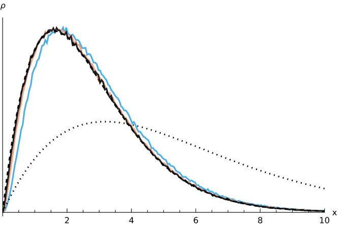
Figure 2: The spectral probability density $\rho_{t}$ in function of the dimensionless frequency $x$ for the Kompaneets process (21), with plots for $t=1,2,3$ going from right to left. The dotted line indicates the initial “hot Planck” condition corresponding to the occupation field $n_{0}(x)=n_{\text{BE}}(x/2)/8$ for which $Z=1$. Notice the fast thermalization to a Wien-like tail, followed by a slow final thermalization at lower frequencies ($x<6$).

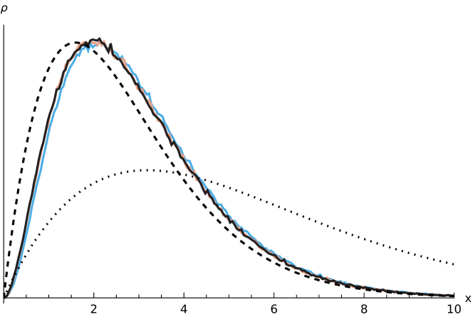
Figure 3: Similar to Fig. 2, but with $Z=0.1$, i.e., with the initial occupation field $n_{0}(x)=n_{\text{BE}}(x/2)/80$. There is a marked difference (going like $x^{2}$ at low frequency) with the dashed line representing the Planck density, as there is particle conservation. There is only the fast thermalization to a(n almost) Wien density because of the absence of low-frequency activity, $x^{2}n_{t}(x)\ll 1$ at low $x$.

If we lower $Z$ to, say, $0.1$, the frequency spectral density instead converges to something closely resembling the Wien distribution $\simeq x^{2}e^{-x}$, as verified in Fig. 3. This corresponds to (4) with $\mu\simeq-2.13$. There is no further convergence to the Planck law here because there is particle conservation and because of the absence of low-frequency drift or diffusion for $x\ll 1$, making both (25) and (26) negligible since $n_{t}(x)$ is of order 1 there.

We conclude from these simulations that the constructed process (21) can be reliably simulated and indeed, for its deterministic behavior reproduces the time-evolution (7), and hence the Kompaneets equation (1). We have given examples of various initial conditions and we conclude that the Kompaneets process shows two different time-scales: one is a fast relaxation to the Planck shape, better at high frequencies, after which a slower relaxation occurs shifting the distribution at the correct temperature. Such a fast prethermalization followed by a slower adjustment is not uncommon in kinetic equations; it already happens in the classical Boltzmann equation where a local Maxwellian is rapidly established.
Finally, we note that when taking $Z>1$, a condensate is expected to form levermore . Fig. 4 shows that condensate appearing for the simulated spectral density for $Z=1.1$. In that case, we also find particles going out of bounds at $x=0$, leading to unphysical negative energies. However, that may be remedied by non-particle-conserving processes (e.g. double Compton or Brehmsstrahlung), which absorb the condensate at the origin (though simulation results are not shown here).

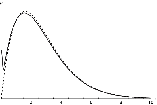
Figure 4: ”Stationary” spectral density for $Z=1.1$. The dashed line is the Planck density. Notice the formation of a condensate around the origin. In that case, there is also the appearance of non-physical negative frequencies. The condensate and the non-physical behavior may be remedied by considering radiative processes like Bremsstrahlung.

V Bremsstrahlung and double Compton scattering

Double Compton scattering and Bremsstrahlung are additional radiation processes, physically similar in controlling emission and absorption of photons. Since the number of photons is not conserved in this case, we can regard them as mechanisms to control the photon number density.
Both can be implemented as stochastic processes but we skip the derivations. We refer to emrmodel ; longair , where the analysis that leads to the master equation was first obtained by Kompaneets (Eq. (18) in kompa ).

The Bremsstrahlung process resembles a chemical reaction, where photons are produced by electrons as they are deflected by nuclei. Here, we use the expression derived by Kompaneets to write in a slightly different manner

$$\left(\frac{\partial n}{\partial t}\right)_{\text{B}}=\frac{\tau_{C}}{\tau_{B}(x)}\left(\frac{1}{e^{x}-1}-n(t,x)\right)$$ (27)

where we have used $\tau_{C}$, the characteristic Compton timescale of (3), to make the comparison with the frequency dependent timescale $\tau_{B}(x)$ of Bremsstrahlung. Notice how there is no diffusion or drift, Bremsstrahlung instead provides a pointwise convergence of the occupation numbers towards the Bose-Einstein distribution.
If we temporarily reinstate units, and assuming for a moment that all nuclei are single protons, which means their density matches that of the electrons, we find that

$$\frac{\tau_{C}}{\tau_{B}(x)}=\frac{9\alpha n_{e}}{8}\mathchoice{{\hbox{$\displaystyle\sqrt{\frac{\pi}{2}\left(\frac{m_{e}c^{2}}{k_{B}T}\right)^{3}\,}$}\lower 0.4pt\hbox{\vrule height=11.74442pt,depth=-9.39557pt}}}{{\hbox{$\textstyle\sqrt{\frac{\pi}{2}\left(\frac{m_{e}c^{2}}{k_{B}T}\right)^{3}\,}$}\lower 0.4pt\hbox{\vrule height=9.30444pt,depth=-7.44359pt}}}{{\hbox{$\scriptstyle\sqrt{\frac{\pi}{2}\left(\frac{m_{e}c^{2}}{k_{B}T}\right)^{3}\,}$}\lower 0.4pt\hbox{\vrule height=6.7222pt,depth=-5.37779pt}}}{{\hbox{$\scriptscriptstyle\sqrt{\frac{\pi}{2}\left(\frac{m_{e}c^{2}}{k_{B}T}\right)^{3}\,}$}\lower 0.4pt\hbox{\vrule height=6.7222pt,depth=-5.37779pt}}}\left(\frac{\hbar c}{k_{B}T}\right)^{3}\frac{\sinh(x/2)K_{0}(x/2)}{x^{3}}$$ (28)

where $\alpha$ is the fine structure constant and $K_{0}$ is a modified Bessel function of the second kind macdon (adapted to our notation from kompa ). Given the $x^{-3}$ dependence of the timescale, we see that Bremsstrahlung dominates the very lowest frequencies, but is negligible everywhere else. Qualitatively, they reproduce the above reactive processes.

Similarly, we can treat the double Compton mechanism, whose radiative nature makes the treatment parallel to Bremsstrahlung. We choose to not give the detailed expression for the timescale, but we follow lightman to note that double Compton scattering is faster in producing the Planck spectrum. In fact, both have nearly the same frequency dependence, but Bremsstrahlung is more relevant for rarefied photon gases and matter-dominated plasmas. Conversely, double Compton scattering becomes more important at higher electron-temperatures and for radiation-dominated plasmas lightman .

Nevertheless, in our simulation of the extened Kompaneets process below, we do not need the detailed implementation of the processes. Using the fact that both radiative mechanisms have “nearly” the same frequency dependence, we control in the simulations the number of photons by hand. Both processes completely dominate the lower frequency ranges, but are negligible compared to Compton scattering for higher frequencies. In the simulations of the Kompaneets process we will simply add or remove particles under a certain cutoff such that their occupation numbers always exactly correspond to the Bose-Einstein distribution for a given volume and temperature.

VI Extension of the Kompaneets process

It is well known that the Boltzmann equation, the traditional point of departure to obtain (1), may wash out certain nonequilibrium degrees of freedom of the electron bath: any isotropic distribution barbosa ; brown ; brown2 ; peebles for the bath (which respects a mild constraint on the decay rate towards zero at infinity)paper yields the Kompaneets equation with a suitable redefinition of the temperature.
As proposed in paper , the Kompaneets equation can be extended to include more general diffusivities and a possible driving. In the present section we directly interfere with the Kompaneets process to add nonequilibrium features to the photon process, leaving aside for a moment the specific origin. There will in fact be two main directions of nonequilibrium, effectively introduced in a generalized Kompaneets equation.

On the level of the Kompaneets equation, the nonequilibrium extension is taken to be

$$\frac{\partial n}{\partial t}=\frac{1}{x^{2}}\frac{\partial}{\partial x}x^{4}\left\{\frac{\partial n}{\partial x}(t,x)+(1+bx^{k})[1+n(t,x)]n(t,x)\right\}+\frac{c}{x^{2}}\frac{\partial}{\partial x}x\left\{\frac{\partial n}{\partial x}(t,x)\right\}$$ (29)

parametrized by positive constants $b,c$ and $k$. As before, we have changed to dimensionless variables. That makes a special case of a more general extended Kompaneets equation

$$x^{2}\frac{\partial n}{\partial t}(t,x)=\frac{\partial}{\partial x}x^{2}D(x)\left\{\frac{\partial n}{\partial x}(t,x)+g(x)[1+n(t,x)]n(t,x)\right\}$$ (30)

for

$$D(x)=x^{2}+\frac{c}{x},\qquad g(x)=\frac{1+bx^{k}}{1+cx^{-3}}$$ (31)

Obviously, the case $c=b=0$ recovers the standard Kompaneets equation. The change in the drift where to the energy function $U(\omega)=\hbar\omega$ (for the standard Kompaneets process) an extra potential $\sim\omega^{k+1}$ is added, is motivated by the search for higher order drivings where the force may depend on the frequency. One is to change the drift, where we imagine a driving that depends on the frequency instead of a constant “force” as in the Kompaneets process. Obviously, we do not assume photon-photon scattering, which is extremely weak in vacuum silveira . The drift can however be realized by employing strong light-matter coupling, resulting in strong effective energy exchanges (and dissipation) on single-photon level roy2 . In other words, we change (22) (or (25)) and replace the constant $U^{\prime}$ with a frequency-dependent force $g$.
A second change is to add an extra diffusion (changing (26)) where the diffusion constant no longer has the features of Compton scattering, but gets modified at low frequencies. By making $c\neq 0$ an extra diffusion has been added in frequency space where the diffusivity decays with frequency, certainly unlike Compton-type processes. Obviously, the dependence $c/x$ in (31) should not be taken literally all the way to $x\downarrow 0$ but an appropriate cutoff will be installed in the simulation (in the next section). In general, while interested in low-frequency effects, we are not interested in the very-low frequency-behavior $x\downarrow 0$. The extra diffusive term (the last term in (29)) was also introduced in arca , motivated by hints of low-frequency modifications in the Planck law, as observed from ARCADE 2 data arcade1 ; arcade2 and EDGES experiment edges . The idea is to drastically increase the activity of low-frequency photons, which are otherwise largely untouched in Compton scattering. Or, in other words, to decrease the activity of high-energy photons. The latter was motivated by a mechanism similar to stochastic turbulence. One should think here of the analogue of creating suprathermal tails in electron velocity distributions by their Rutherford scattering against turbulent fields supra1 ; banerjee . From the Coulomb interaction, high energy electrons are least scattered. Similarly, low-frequency photons are least affected by Compton scattering and that allows them to become abundant by nonequilibrium effects, breaking detailed balance with respect to the Planck law.

A rearrangement is in order to rewrite (30) in terms of the spectral density $\rho(t,x)$, defined in the exact same way as (5), yielding

$$\frac{\partial}{\partial t}\rho(t,x)=-\frac{\partial}{\partial x}\left[\left(2\frac{D(x)}{x}+\partial_{x}D(x)-D(x)g(x)\left(1+n(t,x)\right)\right)\rho(t,x)\right]+\frac{\partial^{2}}{\partial x^{2}}[D(x)\rho(t,x)]$$ (32)

Note the stimulated emission with the occupation number density $n(t,x)$; of course we can subsitute the spectral density from (5). Yet is numbers that matter, not probability.
Observe that (30) remains a continuity equation, photon-number preserving just like Kompaneets. It means that $Z_{t}$ in (5) for the density of the nonequilibrium extension (30) is also a time-independent prefactor, depending only on the environment temperature and the (constant) number of photons per volume.
Interpreting similarly as before the above equation as a Fokker-Planck type equation, we find the associated Langevin equation in the Itô-interpretation

$$\dot{x}=2\frac{D(x)}{x}+\partial_{x}D(x)-D(x)g(x)\left(1+n(t,x)\right)+\mathchoice{{\hbox{$\displaystyle\sqrt{2D(x)\,}$}\lower 0.4pt\hbox{\vrule height=7.5pt,depth=-6.00003pt}}}{{\hbox{$\textstyle\sqrt{2D(x)\,}$}\lower 0.4pt\hbox{\vrule height=7.5pt,depth=-6.00003pt}}}{{\hbox{$\scriptstyle\sqrt{2D(x)\,}$}\lower 0.4pt\hbox{\vrule height=5.25pt,depth=-4.20003pt}}}{{\hbox{$\scriptscriptstyle\sqrt{2D(x)\,}$}\lower 0.4pt\hbox{\vrule height=3.75pt,depth=-3.00002pt}}}\,\xi_{t}$$ (33)

where $\xi_{t}$ is a standard white noise as before. According to (23), we have in this case

$$B(x,\rho_{t})=2\frac{D(x)}{x}+\partial_{x}D(x)-D(x)g(x)\left(1+n(t,x)\right)$$ (34)

with drift and diffusion given by expression (31), and $n(t,x)$ derived from $\rho(t,x)$ as before.

To be compared with (21), the above equation defines the extended Kompaneets process and makes our second main result: it is the fluctuating single-photon dynamics that takes into account physically interesting nonequilibrium features. Note that a stationary solution to (29) can be found, of the form

$$n_{\text{st}}(x;b,c;k)=\frac{1}{\exp\left(\int_{x_{0}}^{x}\differential s\,\frac{1+bs^{k}}{1+cs^{-3}}\right)-1}$$ (35)

where $x_{0}$ is the cutoff for the extra diffusion, as we expect for a realistic situation. That solution is only valid for $x>x_{0}$. For $x\leq x_{0}$ the details of the cutoff should enter in the exponent as to make $n_{\text{st}}$ well defined. When adding radiative processes to (32) at low frequencies such as Bremsstrahlung (see Section V), the stationary solution differs from (35) as well.

VII Simulation of the extended Kompaneets process

Simulations of these extended processes are straightforward, we repeat the algorithm of Section IV, but with different functions $B$ and $D$. Furthermore, we perform an ad hoc implementation of Bremsstrahlung and double Compton scattering, by simply clamping the occupation numbers of the lowest frequencies to the Planck distribution, as explained in Section V. Specifically, we look at the lowest 1% of the frequency range, which in our case consists of the lowest two bins, and compare the empirical occupation number with value expected from the Planck distribution. In case there is an excess, the surplus amount of particles are randomly chosen and removed from the simulation. On the other hand, if there is a deficit, particles are added, randomly distributed over the bin, to make up the difference.
Notice that as particles are being added to or removed from the ensemble, the value of $Z$ will change, i.e, it becomes time-dependent $Z=Z_{t}$.
In the following subsections we separate the influence of $b$ and $c$ in (31); indeed we estimate it is interesting to study their influence separately and the physical mechanisms underlying their presence.

VII.1 Adding low-frequency diffusion

We first take $c=0.1$, leaving $b=0$ in (31). A spurious difficulty arises for nonzero $c$, as the given diffusion and drift coefficients diverge near the origin. To remedy this, we implement a cutoff $x_{0}$ in the simulation, which we take to be $0.1$ (i.e. 1% of the relevant frequency range), where the extra diffusion term is taken to go linearly to zero as $x$ goes below this cutoff, as it is nonphysical for the activity to remain the same all the way to zero frequency anyway.

Simulating with initially $2\text{\times}{10}^{5}$ particles, Fig 5 shows the resulting frequency histogram of the simulation for a total time $\simeq 5$ with the black solid line corresponding to (almost) stationarity. Deviations from the dashed Planckian distribution are evident, with an abundance of low-frequency photons, but keeping the Planck-shape at larger frequency. Together with the extra diffusivity, we implement reactive mechanisms. That makes the behavior below the cutoff frequency $x_{0}$ similar as if we were to turn off the extra diffusive term, i.e, to make $c=0$ for $x<x_{0}$. With that in mind we define

$$h(x)=\int_{0}^{x}\differential x^{\prime}\begin{cases}\frac{1}{1+c/x^{\prime 3}}&\text{for $x^{\prime}>x_{0}$}\\ 1&\text{for $x^{\prime}<x_{0}$}\end{cases}.$$

Then, the stationary distribution appears very well described as

$$n_{\text{st}}(x)=\frac{1}{\exp(h(x))-1}$$ (36)

as is tested in Fig. 5. That theoretical density would correspond to $Z=1.82$, which is however not the value $Z\approx 1.73$ that is found in the simulation. This is not surprising since the addition of reactive processes should make the stationary distribution slightly different at low frequencies.

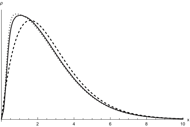
Figure 5: Solid line corresponds to the simulation of (33) using (31) for $c=0.10,b=0$. The dashed line is the Planck law. The dotted line depicts the supposed stationary distribution (36).

Figure 6: Profile of effective temperature corresponding to Fig. 4 and defined in (37). The very-low frequency regime is dominated by the ad hoc cutoff and procedures replacing Bremsstrahlung and double Compton scattering, as explained in the text. For low frequency $1<x<5$ the effective temperature is significantly higher than the Planck-value.

We define an effective temperature $T_{\text{eff}}(x)$ as a function of the frequency, derived from the empirical occupation number at this frequency by inverting the Planck distribution,

$$n_{\text{Pl},T_{\text{eff}}}(x)=\frac{1}{\exp(x/T_{\text{eff}})-1}$$ (37)

Because of our choice of units, this will be expressed as a ratio to the temperature of the background electron gas. Fig. 6 plots this effective temperature for the stationary distribution.

VII.2 Adding frequency-dependent drift

Taking now a non-zero driving in (31), we set $b=0.1$ and $k=0.4$, keeping $c=0$. A marked deviation from the Planck law becomes visible. It is also interesting to note a remarkable feature for $b\neq 0$, which is the formation of a condensate around $x=0$. However, the low-frequency reaction mechanism (either double Compton or Bremssthralung) is able to absorb the condensate. In fact, the appearance of that condensate can be explained by looking at the stochastic equation (33), where the extra drift coming from $g(x)$ contributes in the stimulated emission term, making shifts towards negatives values of frequency more frequent.

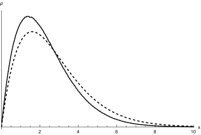
Figure 7: Stationary density profile when adding the frequency-dependent drift with $b=0.1$ and $k=0.4$, keeping $c=0$ in (31). Again a deviation is seen from the Planck law (dashed line), with the simulation almost completely overlapping with the stationary solution.

Here, in contrast with the diffusive addition in Fig. 5, high frequencies get much more affected.

VIII Conclusions

The present paper achieves to construct photon processes in frequency space dominated by Compton scattering. The stimulated emission produces the nonlinearities. From the single-photon stochastic process, we enter the realm of time-dependent fluctuation phenomena for photon dynamics. It implies we can start exploring nonequilibrium photon dynamics, much in the tradition of stochastic dynamics for open particle systems. We have explored the addition of nonequilibrium drift and diffusion terms which affect mostly the low-frequency part in a modified Planck spectrum.

Various applications can be envisaged, subject of future studies, while the present paper sets the mathematical and simulational structure of the photon diffusion process. Despite the appearance of nonlinearities, due to stimulated emission, which makes a nontrivial aspect, we simulate this process using traditional algorithms for stochastic equations and conclude that relaxation to the equilibrium Planck law can be reliable simulated, as seen in Fig. 2. The nonlinearity is satisfactorily dealt by considering an ensemble of processes while using histograms to construct the empirical spectral density of photons at each time step. Physical processes such as Bremsstrahlung and double Compton can also be easily included by an ad hoc procedure we describe in Section V. It means to continuously set, below some cutoff frequency, the density of photons to its corresponding value in the Planck spectrum, under the argument that low-frequency photons rapidly thermalize via reactive mechanisms.

The $Z$ parameter can be tuned as to make the stimulated emission weaker and convergence to a Wien-like spectrum is observed in the simulations; see Fig. 3. In fact, this would correspond to a rarefied photon gas, where stimulated emission is expected to become less important. On the other hand, detailed balance with respect to Planck’s law is broken by considering the extension to the Kompaneets equation. There, nonequilibrium drift and diffusion make extra contributions to the standard equation for the single-photon process. The proposed extension (29) is parameterized by the values $b,c$ and $k$, such that $b=c=0$ corresponds to the standard Kompaneets process (21). The simulation results, Figs. 5 and 7, show that, for the values of parameters considered, modifications to the Planck law that ultimately lead to higher occupancy in the low-frequency part of the spectrum are seen. Those modifications match very well with the theoretical stationary solution (36), but slight deviations are expected due to the inclusion of reaction mechanisms.
From the mathematical point of view, the derivation of the Kompaneets process is interesting and challenging. It appears to open a new theme in the domain of nonlinear Markov diffusions fra .
Let us finish by emphasizing that the proposed mechanisms remain conjectural and that the theory is largely phenomenological. A follow-up can be found in res , where a resetting mechanism is added to the Kompaneets process corresponding to random abrupt Doppler shifts to the low frequency regime.

Appendix A Itô’s lemma and the Kompaneets process

Suppose we have a (possibly) time-dependent function of the random variable $\mathbf{X}_{t}$

$$f=f(t,\mathbf{X}_{t})$$

then, $f$ itself is a random variable. Suppose also that $\mathbf{X}_{t}$ follows the stochastic differential equation

$$\dot{\mathbf{X}}_{t}=\mathbf{B}(\mathbf{X}_{t})+\mathbf{Q}_{t}(\mathbf{X}_{t})\mathbf{\Xi}_{t}$$

where $\mathbf{\Xi}_{t}$ is a three-dimensional white noise as before.

Then, Itô’s lemma states that $f$ satisfies the stochastic differential equation

$$\dot{f}(t,\mathbf{X}_{t})=\frac{\partial f}{\partial t}+\left(\nabla_{\mathbf{X}}f\right)\cdot\mathbf{B}+\frac{1}{2}\mathrm{Tr}\left[\mathbf{Q}^{T}_{t}\left(H_{X}f\right)\mathbf{Q}_{t}\right]+\left(\nabla_{\mathbf{X}}f\right)^{T}\mathbf{Q}_{t}\,\mathbf{\Xi}_{t}$$ (38)

where the positive $d\times d$ matrix $\mathbf{Q}_{t}$ is such that the diffusion tensor

$$\mathbf{D}=\frac{1}{2}\mathbf{Q}_{t}\mathbf{Q}^{T}_{t}$$

and $H_{X}$ is the Hessian matrix with respect to $\mathbf{X}_{t}$.

We use that to show in more detail the derivation of equation (21). We begin with the $i$-th generator in (15)

$$\frac{1}{\delta^{2}}{L_{i}}_{\delta}F(\mathbf{K})=D(\mathbf{k}_{i})(1+n_{\mathbf{k}_{i}}(\mathbf{K}))\Delta_{\mathbf{k}_{i}} F(\mathbf{K})+\sum_{\mathbf{a}}\bigg{\{}\left(\frac{1}{2}\mathbf{a}\cdot\nabla_{\mathbf{k}}D(\mathbf{k}_{i})-\frac{\beta}{2}D(\mathbf{k}_{i})\mathbf{a}\cdot\nabla_{\mathbf{k}}U(\mathbf{k}_{i})\right)$$

$$(1+n_{\mathbf{k}_{i}}(\mathbf{K}))\ +D(\mathbf{k}_{i})\,\mathbf{a}\cdot\nabla_{\mathbf{k}}n\bigg{\}}\mathbf{a}\cdot\nabla_{\mathbf{k}_{i}}F(\mathbf{K})$$ (39)

which leads by applying the steps (16)–(19) to the Itô process for the $i$-th photon

$$\dot{\mathbf{k_{i}}}_{t}=\nabla_{\mathbf{k}}{D}({\mathbf{k_{i}}_{t}})-\beta D(\mathbf{k_{i}}_{t})\,\nabla_{\mathbf{k}}U(\mathbf{k_{i}}_{t})(1+n_{\mathbf{k_{i}}_{t}}(\mathbf{K}))+\mathchoice{{\hbox{$\displaystyle\sqrt{2D(\mathbf{{k_{i}}_{t}})\,}$}\lower 0.4pt\hbox{\vrule height=7.5pt,depth=-6.00003pt}}}{{\hbox{$\textstyle\sqrt{2D(\mathbf{{k_{i}}_{t}})\,}$}\lower 0.4pt\hbox{\vrule height=7.5pt,depth=-6.00003pt}}}{{\hbox{$\scriptstyle\sqrt{2D(\mathbf{{k_{i}}_{t}})\,}$}\lower 0.4pt\hbox{\vrule height=5.25pt,depth=-4.20003pt}}}{{\hbox{$\scriptscriptstyle\sqrt{2D(\mathbf{{k_{i}}_{t}})\,}$}\lower 0.4pt\hbox{\vrule height=3.75pt,depth=-3.00002pt}}}\,\mathbf{\Xi}_{t}$$ (40)

In order to simplify notation, we will opt to not differentiate the quantities from their dimensionless counterpart, therefore, it should be noted that all quantities appearing here are dimensionless. In particular, we shall identify the photon energy with its dimensionless version

$$\beta U(\omega_{i})\to U(x_{i})=x_{i}$$

We apply Itô’s lemma for

$$f(\mathbf{k_{i}})=|\mathbf{k_{i}}|.$$

A simple calculation yields

$$\nabla_{\mathbf{k_{i}}}f=\frac{\mathbf{k_{i}}}{|\mathbf{k_{i}}|}$$

$$H_{\mathbf{k_{i}}}f=\begin{pmatrix}\frac{1}{|\mathbf{k_{i}}|}-\frac{{k_{ix}}^{2}}{|\mathbf{k_{i}}|^{3}}&&\\ &\frac{1}{|\mathbf{k_{i}}|}-\frac{{k_{iy}}^{2}}{|\mathbf{k_{i}}|^{3}}&\\ &&\frac{1}{|\mathbf{k_{i}}|}-\frac{{k_{iz}}^{2}}{|\mathbf{k_{i}}|^{3}}\end{pmatrix}$$

recall from (40) that

$$\mathbf{B}(\mathbf{k_{i}})=\nabla_{\mathbf{k}}D(\mathbf{k_{i}})-D(\mathbf{k_{i}})\nabla_{\mathbf{k}}{U}(\mathbf{k_{i}})(1+n_{\mathbf{k_{i}}}(\mathbf{K}))$$

$$\mathbf{Q}(\mathbf{k_{i}})=\mathchoice{{\hbox{$\displaystyle\sqrt{2D(\mathbf{k_{i}})\,}$}\lower 0.4pt\hbox{\vrule height=7.5pt,depth=-6.00003pt}}}{{\hbox{$\textstyle\sqrt{2D(\mathbf{k_{i}})\,}$}\lower 0.4pt\hbox{\vrule height=7.5pt,depth=-6.00003pt}}}{{\hbox{$\scriptstyle\sqrt{2D(\mathbf{k_{i}})\,}$}\lower 0.4pt\hbox{\vrule height=5.25pt,depth=-4.20003pt}}}{{\hbox{$\scriptscriptstyle\sqrt{2D(\mathbf{k_{i}})\,}$}\lower 0.4pt\hbox{\vrule height=3.75pt,depth=-3.00002pt}}}\mathbf{I}_{3\times 3}$$

Therefore, we can easily find all terms in Itô’s lemma (38)

$$\begin{cases}&\partial_{t}f=0\\ &\left(\nabla_{\mathbf{X}}f\right)\cdot\mathbf{B}=\frac{\mathbf{k_{i}}}{|\mathbf{k_{i}}|}\cdot\left(\nabla_{\mathbf{k}}D(\mathbf{k_{i}})-D(\mathbf{k_{i}})\nabla_{\mathbf{k}}{U}(\mathbf{k_{i}})(1+n_{\mathbf{k_{i}}}(\mathbf{K}))\right)\\ &\frac{1}{2}\mathrm{Tr}\left[\mathbf{Q}^{T}_{t}\left(H_{X}f\right)\mathbf{Q}_{t}\right]=2\frac{D(\mathbf{k_{i}})}{|\mathbf{k_{i}}|}\\ &\left(\boldsymbol{\nabla_{X}}f\right)^{T}\mathbf{Q}_{t}=\mathchoice{{\hbox{$\displaystyle\sqrt{2D(\mathbf{k_{i}})\,}$}\lower 0.4pt\hbox{\vrule height=7.5pt,depth=-6.00003pt}}}{{\hbox{$\textstyle\sqrt{2D(\mathbf{k_{i}})\,}$}\lower 0.4pt\hbox{\vrule height=7.5pt,depth=-6.00003pt}}}{{\hbox{$\scriptstyle\sqrt{2D(\mathbf{k_{i}})\,}$}\lower 0.4pt\hbox{\vrule height=5.25pt,depth=-4.20003pt}}}{{\hbox{$\scriptscriptstyle\sqrt{2D(\mathbf{k_{i}})\,}$}\lower 0.4pt\hbox{\vrule height=3.75pt,depth=-3.00002pt}}}\frac{\mathbf{k_{i}}}{|\mathbf{k_{i}}|}\end{cases}$$

we substitute back in (38) and write quantities in terms of the dimensionless frequency $\mathbf{k_{i}}=x_{i}\,\mathbf{\hat{x_{i}}}$. Repeating the process for $i=1,\dots,N$, taking the sum and the continuum limit for the generator in frequency space similarly than done in steps (15)–(19) we find (21).
Applying directly Itô’s lemma for a nonlinear Markov diffusion is not needed here, but is another mathematical question that is raised by the Kompaneets process.

Appendix B Data Availability Statement

The data and software that support the findings of this study are openly available on GitLabgitlab .

References

- (1) J. Koch, A. A. Houck, K. L. Hur, and S. M. Girvin, “Time-reversal-symmetry breaking in circuit-qed-based photon lattices,” Phys. Rev. A, vol. 82, p. 043811, Oct. 2010.
- (2) K. Fang, Z. Yu, and S. Fan, “Realizing effective magnetic field for photons by controlling the phase of dynamic modulation,” Nature Photonics, vol. 6, pp. 782–787, Nov. 2012.
- (3) P. Roushan, C. Neill, A. Megrant, Y. Chen, R. Babbush, R. Barends, B. Campbell, Z. Chen, B. Chiaro, A. Dunsworth, A. Fowler, E. Jeffrey, J. Kelly, E. Lucero, J. Mutus, P. J. J. O’Malley, M. Neeley, C. Quintana, D. Sank, A. Vainsencher, J. Wenner, T. White, E. Kapit, H. Neven, and J. Martinis, “Chiral ground-state currents of interacting photons in a synthetic magnetic field,” Nature Physics, vol. 13, pp. 146–151, Oct. 2016.
- (4) D. Pozar, Microwave Engineering. Wiley, 2004.
- (5) D. Roy, “Two-photon scattering by a driven three-level emitter in a one-dimensional waveguide and electromagnetically induced transparency,” Phys. Rev. Lett., vol. 106, p. 053601, Feb. 2011.
- (6) A. Baev, P. N. Prasad, H. Ågren, M. Samoć, and M. Wegener, “Metaphotonics: An emerging field with opportunities and challenges,” Physics Reports, vol. 594, pp. 1–60, 2015. Metaphotonics: An emerging field with opportunities and challenges.
- (7) T. Demaerel, W. De Roeck, and C. Maes, “Producing suprathermal tails in the stationary velocity distribution,” Physica A: Statistical Mechanics and its Applications, vol. 552, p. 122179, 2020. Tributes of Non-equilibrium Statistical Physics.
- (8) T. Banerjee, U. Basu, and C. Maes, “Active velocity processes with suprathermal stationary distributions and long-time tails,” Phys. Rev. E, vol. 101, p. 062130, June 2020.
- (9) E. Fermi, “On the origin of the cosmic radiation,” Phys. Rev., vol. 75, pp. 1169–1174, Apr. 1949.
- (10) P. A. Sturrock, “Stochastic acceleration,” Phys. Rev., vol. 141, pp. 186–191, Jan. 1966.
- (11) C. Univ, M. Brin, W. on Dynamical Systems, R. Topics, K. Burns, D. Dolgopyat, and Y. Pesin, Fermi acceleration, p. 149. Contemporary mathematics - American Mathematical Society, American Mathematical Society, 2008.
- (12) T. Buchert, “Dark Energy from structure: a status report,” General Relativity and Gravitation, vol. 40, pp. 467–527, Dec. 2007.
- (13) D. J. Fixsen, A. Kogut, S. Levin, M. Limon, P. Lubin, P. Mirel, M. Seiffert, J. Singal, E. Wollack, T. Villela, and C. A. Wuensche, “ARCADE 2 Measurement of the Absolute Sky Brightness at 3-90 GHz,” Astrophys. J. , vol. 734, p. 5, June 2011.
- (14) M. Seiffert, D. J. Fixsen, A. Kogut, S. M. Levin, M. Limon, P. M. Lubin, P. Mirel, J. Singal, T. Villela, E. Wollack, and C. A. Wuensche, “Interpretation of the ARCADE 2 absolute sky brightness measurement,” The Astrophysical Journal, vol. 734, p. 6, may 2011.
- (15) K. Cheung, J.-L. Kuo, K.-W. Ng, and Y.-L. S. Tsai, “The impact of EDGES 21-cm data on dark matter interactions,” Physics Letters B, vol. 789, pp. 137–144, 2019.
- (16) M. Baiesi, C. Burigana, L. Conti, G. Falasco, C. Maes, L. Rondoni, and T. Trombetti, “Possible nonequilibrium imprint in the cosmic background at low frequencies,” Phys. Rev. Research, vol. 2, p. 013210, Feb. 2020.
- (17) A. S. Kompaneets, “The Establishment of Thermal Equilibrium between Quanta and Electrons,” Soviet Journal of Experimental and Theoretical Physics, vol. 4, pp. 730–737, May 1957.
- (18) C. D. Levermore, H. Liu, and R. L. Pego, “Global dynamics of bose–einstein condensation for a model of the kompaneets equation,” SIAM Journal on Mathematical Analysis, vol. 48, no. 4, pp. 2454–2494, 2016.
- (19) D. A. Liedahl, The X-Ray Spectral Properties of Photoionized Plasma and Transient Plasmas, vol. 520, p. 189. 1999.
- (20) R. D. Blandford and E. T. Scharlemann, “On induced Compton scattering by relativistic particles,” Astrophysics and Space Science, vol. 36, pp. 303–317, Sept. 1975.
- (21) R. A. Sunyaev and Y. B. Zeldovich, “Distortions of the background radiation spectrum,” Nature, vol. 223, pp. 721–722, Aug. 1969.
- (22) R. A. Sunyaev and Y. B. Zeldovich, “The Observations of Relic Radiation as a Test of the Nature of X-Ray Radiation from the Clusters of Galaxies,” Comments on Astrophysics and Space Physics, vol. 4, p. 173, Nov. 1972.
- (23) D. G. Shirk, “A practical review of the kompaneets equation and its application to Compton scattering,” 2006.
- (24) G. E. Freire Oliveira, “Statistical mechanics of the Kompaneets equation,” Master’s thesis, KU Leuven. Faculteit Wetenschappen, Leuven, 2021.
- (25) Y. B. Zeldovich, “Interaction of free electrons with electromagnetic radiation,” Soviet Physics Uspekhi, vol. 18, pp. 79–98, Feb. 1975.
- (26) C. Buet, B. Després, and T. Leroy, “Anisotropic models and angular moments methods for the Compton scattering.” working paper or preprint, Feb. 2018.
- (27) C. Pitrou, “Radiative transport of relativistic species in cosmology,” Astroparticle Physics, p. 102494, 2020.
- (28) D. Barbosa, “A note on Compton scattering,” The Astrophysical Journal, vol. 254, pp. 301–308, 1982.
- (29) L. S. Brown and D. L. Preston, “Leading relativistic corrections to the kompaneets equation,” Astroparticle Physics, vol. 35, no. 11, pp. 742–748, 2012.
- (30) N. Itoh, Y. Kohyama, and S. Nozawa, “Relativistic corrections to the Sunyaev-Zeldovich effect for clusters of galaxies,” The Astrophysical Journal, vol. 502, no. 1, p. 7, 1998.
- (31) N. Itoh and S. Nozawa, “Relativistic corrections to the Sunyaev-Zeldovich effect for extremely hot clusters of galaxies,” A&A, vol. 417, no. 3, pp. 827–832, 2004.
- (32) G. Cooper, “Compton Fokker-Planck equation for hot plasmas,” Physical Review D, vol. 3, no. 10, p. 2312, 1971.
- (33) S. Nozawa and Y. Kohyama, “Analytical study on the Sunyaev-Zeldovich effect for clusters of galaxies,” Physical Review D, vol. 79, no. 8, p. 083005, 2009.
- (34) S. Nozawa, Y. Kohyama, and N. Itoh, “Analytical study on the Sunyaev-Zeldovich effect for clusters of galaxies. ii. comparison of covariant formalisms,” Physical Review D, vol. 82, no. 10, p. 103009, 2010.
- (35) S. Nozawa and Y. Kohyama, “Relativistic corrections to the kompaneets equation,” Astroparticle Physics, vol. 62, pp. 30–32, 2015.
- (36) G. E. Freire Oliveira, C. Maes, and K. Meerts, “On the derivation of the Kompaneets equation,” Astroparticle Physics, vol. 133, p. 102644, 2021.
- (37) O. Kavian, “Remarks on the Kompaneets equation, a simplified model of the Fokker-Planck equation,” in Nonlinear Partial Differential Equations and their Applications - Collège de France Seminar Volume XIV, pp. 469–487, Elsevier, 2002.
- (38) L. P. Kadanoff, Quantum statistical mechanics. CRC Press, 2018.
- (39) R. A. Blythe and M. R. Evans, “Nonequilibrium steady states of matrix-product form: a solver's guide,” Journal of Physics A: Mathematical and Theoretical, vol. 40, pp. R333–R441, Oct. 2007.
- (40) C. Cocozza-Thivent, “Processus des misanthropes,” Zeitschrift für Wahrscheinlichkeitstheorie und Verwandte Gebiete, vol. 70, no. 4, pp. 509–523, 1985.
- (41) S. Sethuraman, “On diffusivity of a tagged particle in asymmetric zero-range dynamics,” 2004.
- (42) M. Jara, C. Landim, and S. Sethuraman, “Nonequilibrium fluctuations for a tagged particle in one-dimensional sublinear rate zero-range processes,” 2010.
- (43) T. D. Frank, Nonlinear Fokker-Planck equations: fundamentals and applications. Springer Science & Business Media, 2005.
- (44) V. N. Kolokoltsov, Nonlinear Markov Processes and Kinetic Equations. Cambridge Tracts in Mathematics, Cambridge University Press, 2010.
- (45) T. D. Frank, “Strongly nonlinear stochastic processes in physics and the life sciences,” ISRN Mathematical Physics, vol. 2013, pp. 1–28, Mar. 2013.
- (46) T. Funaki, “A certain class of diffusion processes associated with nonlinear parabolic equations,” Zeitschrift für Wahrscheinlichkeitstheorie und Verwandte Gebiete, vol. 67, no. 3, pp. 331–348, 1984.
- (47) H. P. McKean, “A class of Markov processes associated with nonlinear parabolic equations,” Proceedings of the National Academy of Sciences, vol. 56, pp. 1907–1911, Dec. 1966.
- (48) E. Pechersky, A. Yambartsev, and V. Zagrebnov, “Stochastic dynamics of Einstein matter-radiation model with spikes,” 2018.
- (49) M. S. Longair, High energy astrophysics. Cambridge university press, 2010.
- (50) K. B. Oldham, J. C. Myland, and J. Spanier, The Macdonald Function Kv(x), pp. 527–536. New York, NY: Springer US, 2009.
- (51) A. P. Lightman, “Double Compton emission in radiation dominated thermal plasmas,” Astrophys. J. , vol. 244, pp. 392–405, Mar. 1981.
- (52) L. S. Brown, “Compton scattering in a plasma,” Annals of Physics, vol. 200, no. 1, pp. 190–205, 1990.
- (53) P. J. E. Peebles, L. A. Page Jr, and R. B. Partridge, Finding the Big Bang. Cambridge University Press, 2009.
- (54) D. d’Enterria and G. G. da Silveira, “Observing light-by-light scattering at the large hadron collider,” Physical Review Letters, vol. 111, no. 8, 2013.
- (55) D. Roy, C. M. Wilson, and O. Firstenberg, “Colloquium: Strongly interacting photons in one-dimensional continuum,” Rev. Mod. Phys., vol. 89, p. 021001, May 2017.
- (56) G. E. F. Oliveira, C. Maes, and K. Meerts, “Resetting photons,” 2022.
- (57) K. Meerts, “Photon diffusion process.” https://gitlab.kuleuven.be/u0131889/photon-diffusion-process/-/tags/v1.0.