Scalable spin squeezing from spontaneous breaking of a continuous symmetry

Abstract

Spontaneous symmetry breaking (SSB) is a property of Hamiltonian equilibrium states which, in the thermodynamic limit, retain a finite average value of an order parameter even after a field coupled to it is adiabatically turned off. In the case of quantum spin models with continuous symmetry, we show that this adiabatic process is also accompanied by the suppression of the fluctuations of the symmetry generator – namely, the collective spin component along an axis of symmetry. In systems of $S=1/2$ spins or qubits, the combination of the suppression of fluctuations along one direction and of the persistence of transverse magnetization leads to spin squeezing – a much sought-after property of quantum states, both for the purpose of entanglement detection as well as for metrological uses. Focusing on the case of XXZ models spontaneously breaking a U(1) (or even SU(2)) symmetry, we show that the adiabatically prepared states have nearly minimal spin uncertainty; that the minimum phase uncertainty that one can achieve with these states scales as $N^{-3/4}$ with the number of spins $N$; and that this scaling is attained after an adiabatic preparation time scaling linearly with $N$. Our findings open the door to the adiabatic preparation of strongly spin-squeezed states in a large variety of quantum many-body devices including e.g. optical lattice clocks.

Introduction. Many-body entanglement is at the heart of the fundamental complexity of quantum states Preskill (2012), and it is the basis mechanism by which a quantum many-body system relaxes to a stationary state after having been driven away from equilibrium Kaufman et al. (2016). In this respect, the generation of many-body entangled quantum states is one of the main goals of a new generation of quantum devices, going from quantum simulators Georgescu et al. (2014) to quantum computers Nielsen and Chuang (2000), whose common trait is the ability to perform coherent unitary evolutions of quantum many-body systems. Yet, certifying (let alone putting to use) many-body entanglement is a task which is restricted to a small class of quantum many-body states, most prominently those whose entanglement can be detected via the measurement of the lowest moments of the quantum-noise distribution Gühne and Tóth (2009). In the context of ensembles of $N$ qubits ($S=1/2$ spins), characterized by the collective-spin operator ${\bm{J}}=\sum_{i=1}^{N}{\bm{S}}_{i}$ (where the ${\bm{S}}_{i}$’s are $S=1/2$ quantum spin operators), one of the best example of such states is offered by spin-squeezed ones, whose entanglement is detected via the spin-squeezing parameter Wineland et al. (1994)

$$\xi_{R}^{2}=\frac{N\min_{\perp}{\rm Var}(J^{\perp})}{\langle{\bm{J}}\rangle^{2}},$$ (1)

where $\min_{\perp}$ expresses the minimization of the variance on the collective-spin components perpendicular to the average spin orientation $\langle{\bm{J}}\rangle$. A state with $\xi_{R}^{2}<1/k$ $(k\geq 1)$ is entangled, with an entanglement depth (least number of entangled spins) of $k+1$ Sørensen et al. (2001); Pezzè et al. (2018). The $\xi_{R}^{2}$ parameter is also a fundamental figure of merit of the sensitivity of the state to rotations, expressing the reduction in phase-estimation error for a Ramsey interferometric protocol with respect to a factorized state Wineland et al. (1994); and it offers the possibility to improve the efficiency of quantum devices such as atomic clocks Louchet-Chauvet et al. (2010); Leroux et al. (2010a); Pedrozo-Peñafiel et al. (2020); Schulte et al. (2020) or quantum sensors Muessel et al. (2014); Salvi et al. (2018); Shankar et al. (2019) by using entanglement as a resource.

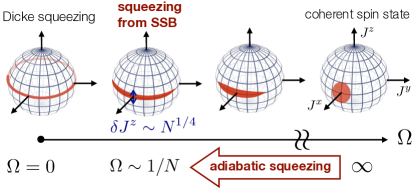
Figure 1: Adiabatic squeezing from spontaneous symmetry breaking in the XXZ model. Starting from a coherent spin state at $\Omega=\infty$, an adiabatic reduction of the field $\Omega$ coupling to the order parameter leads to the appearance of scalable spin squeezing when $\Omega\sim 1/N$, due to the scaling of the uncertainty on the $J^{z}$ component, $\delta J^{z}=\sqrt{{\rm Var}(J^{z})}\sim N^{1/4}$; and to the absence of scaling of the order parameter $m=\langle J^{x}\rangle/N$, as a consequence of spontaneous symmetry breaking (SSB). The red areas depict the uncertainty regions of the collective spin on a sphere of radius $\sqrt{\langle\bm{J}^{2}\rangle}\sim N$. As a consequence the angular aperture of the uncertainty region along the $z$ axis is $\delta\phi\approx\delta J^{z}/\sqrt{\langle\bm{J}^{2}\rangle}\sim N^{-3/4}$, defining the sensitivity of the state to rotations around the $y$ axis.

Figure 2: Adiabatic squeezing from SSB in the 2$d$ Heisenberg model. (a) Field-induced magnetization $\langle J^{x}\rangle/N$ for various lattice sizes $N=L^{2}$; (b) Variance of the collective spin component $J^{z}$; (c) resulting spin-squeezing parameter $\xi_{R}^{2}$; (d) comparison between $\xi_{R}^{-2}$ and $4{\rm Var}(J^{y})/N$. In all panels the solid black line indicates the prediction of linear spin-wave (LSW) theory, and the dotted line in panels (b)-(c) shows the $\Omega^{1/2}$ scaling as a reference (multiplied by an arbitrary prefactor).

For the reasons listed above, devising many-body mechanisms that lead to the controlled preparation of spin-squeezed states Ma et al. (2011) is a very significant endeavor – and particularly so when the squeezing parameter can be parametrically reduced by increasing the number of resources. This situation leads to scalable squeezing – generically $\xi^{2}_{R}\sim N^{-\alpha}$ ($\alpha>0$) – which allows one to surpass the standard quantum limit for the scaling of the phase-estimation error with the number of qubits Pezzè et al. (2018). The two main mechanisms that have been identified and implemented so far in this direction are the preparation of spin-squeezed states via unitary evolutions with collective-spin interactions Kitagawa and Ueda (1993); Estève et al. (2008); Riedel et al. (2010); Bohnet et al. (2016) and via the non-demolition measurement of a spin component Leroux et al. (2010b); Hosten et al. (2016). Yet a third way to spin squeezing is offered by adiabatic preparation, which relies upon the identification of spin squeezing in the ground state of quantum spin Hamiltonians implemented e.g. by quantum simulation platforms. A clear example in this direction is offered by Ising quantum critical points, which exhibit scalable squeezing at and above the upper critical dimension ($d\geq 3$ for short-range interactions) Frérot and Roscilde (2018).

In this work we unveil another fundamental link between many-body physics of spin models and the generation of spin squeezing, namely the appearance of squeezing in the presence of spontaneous breaking of a continuous spin symmetry in the ground state. Without loss of generality, in the following we will be concerned with symmetry under U(1) rotations $U_{z}(\phi)=e^{-i\varphi J^{z}}$ generated by the collective spin component $J^{z}$ – this property is also present for SU(2)-symmetric Hamiltonians. On a finite-size system and in the absence of any symmetry-breaking field, the ground state of a U(1) symmetric Hamiltonian has ${\rm Var}(J^{z})=0$, namely it exhibits so-called Dicke squeezing Pezzè et al. (2018), lacking nonetheless a finite net magnetization $\langle{\bm{J}}\rangle=0$. At the same time, the low-lying energy spectrum of that same Hamiltonian exhibits a so-called Anderson tower of states (ToS), whose energy collapses as $1/N$ onto that of the ground state Anderson (1997); Tasaki (2018); Beekman et al. (2019); Comparin et al. (2021). Hence a field $\Omega\sim 1/N$ coupling to the order parameter in the $x-y$ plane, e.g. $-\Omega J^{x}$ (without loss of generality), is sufficient to mix the ToS into a state exhibiting a net polarization $m=\langle J^{x}\rangle/N\neq 0$. The hallmark of spontaneous symmetry breaking (SSB) is then the persistence of a finite order parameter $m$ in the limit $N\to\infty$, in which the field is also parametrically set to zero. Here we investigate paradigmatic XXZ models with nearest-neighbor interactions using finite-temperature and variational quantum Monte Carlo simulations, as well as of spin-wave theory; and, in the presence of SSB in the ground state, we show that the state polarized by the minimal field $\Omega\sim 1/N$ away from Dicke squeezing retains a strong asymmetry in the fluctuations of the collective spin components, exhibiting scalable (Wineland) spin squeezing with $\xi_{R}^{2}\sim N^{-1/2}$. Such a state is shown to have minimal spin uncertainty, namely squeezing is its optimal metrological resource; and it can be prepared adiabatically, starting from a coherent spin state stabilized at $\Omega\to\infty$, and ramping down $\Omega$ to a value $\sim 1/N$ in a time scaling linearly with system size, $\tau\sim N$ (see Fig. 1 for a summarizing sketch). This finding opens the possibility to squeeze the collective spin of quantum simulators of U(1)- (or SU(2)-)symmetric qubit Hamiltonians, with potential applications to quantum sensors Muessel et al. (2014); Facon et al. (2016) and atomic clocks Takamoto et al. (2005); Campbell et al. (2017).

Model and methods. We focus our attention on the $S=1/2$ XXZ Hamiltonian:

$${\cal H}=-\frac{1}{2}\sum_{ij}{\cal J}_{ij}(S^{x}_{i}S^{x}_{j}+S^{y}_{i}S^{y}_{j}-\Delta S^{z}_{i}S^{z}_{j})-\Omega\sum_{i}\epsilon_{i}S_{i}^{x}$$ (2)

where $i,j$ are lattice sites on a $d$-dimensional hypercubic lattice of size $N=L^{d}$ with periodic boundary conditions. In the following we shall specialize our attention to nearest-neighbor (n.n.) interactions – ${\cal J}_{ij}={\cal J}$ if $i$ n.n. $j$. Moreover we choose ${\cal J}>0$ and $-1<\Delta\leq 1$, defining an XXZ model with ferromagnetic interactions in the plane and ferromagnetic or antiferromagnetic along the symmetry axis. Such a situation is realized e.g. in bosonic Mott insulators Duan et al. (2003); Jepsen et al. (2020); Sun et al. (2021). Under these assumptions, the above model is known to break a continuous symmetry in the ground state in $d\geq 2$; and the field coupling to the order parameter is uniform, namely $\epsilon_{i}=1~{}\forall i$. But most of our results are completely general, and apply to any model featuring SSB of a continuous symmetry – provided that the order parameter does not commute with the Hamiltonian (otherwise the ground state is simply a coherent spin state for all $\Omega$, e.g. $\otimes_{i=1}^{N}|\rightarrow_{x}\rangle_{i}$ with $|\rightarrow_{x}\rangle_{i}$ the eigenstate of $S_{i}^{x}$ with eigenvalue $+1/2$). In the case ${\cal J}<0$ (antiferromagnetic interactions in the $xy$ plane) – as realized in fermionic Mott insulators Duan et al. (2003); Greif et al. (2013); Mazurenko et al. (2017) – the order parameter is the staggered magnetization, e.g. $m=\langle J^{x}_{\rm st}\rangle/N=\langle\sum_{i}\epsilon_{i}S_{i}^{x}\rangle/N$; the field coupling to the order parameter must therefore be staggered, $\epsilon_{i}=(-1)^{i}$; and the relevant rotations are generated by $J^{y}_{\rm st}=\sum_{i}\epsilon_{i}S_{i}^{y}$. Yet, for n.n. interactions on a hypercubic lattice, the physics is equivalent to that of the bosonic insulators, as the two models are connected by a canonical transformation (rotation of $\pi$ around the $z$ axis for one of the two sublattices).

We have studied the ground-state physics of the XXZ Hamiltonian in $d=1,2$ and 3 making use of numerically exact quantum Monte Carlo (QMC) simulations, based on the Stochastic Series Expansion method Syljuåsen and Sandvik (2002); as well as of spin-wave theory, valid in the presence of spontaneous symmetry breaking ($d=2,3$). Moreover we have investigated the (quasi-)adiabatic dynamics of preparation of the ground state starting from a large $\Omega$ by making use of time-dependent variational Monte Carlo (tVMC), based on pair-product (or spin-Jastrow) wavefunctions Thibaut et al. (2019); Comparin et al. (2021) as well as of time-dependent spin-wave theory (see the Supplemental Material – SM – for an extended discussion of the methods SM ).

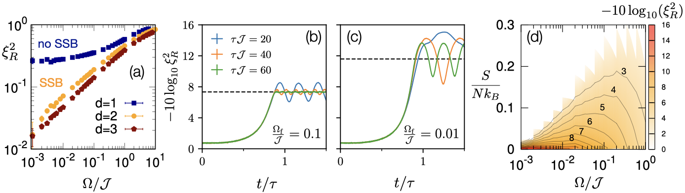
Figure 3: Quasi-adiabatic preparation of the low-field state. (a) Comparison between the field dependence of the squeezing parameter $\xi_{R}^{2}$ for the ground state of the Heisenberg model in $d=$1, 2, and 3. For each value of $\Omega$, we use a system size $N$ such that $\Omega\geq{\cal J}/N$, at a temperature $T/{\cal J}=1/N$ removing thermal effects. (b-c) The two panels show tVMC results for the evolution of the spin-squeezing parameter in the 2$d$ Heisenberg model ($L=12$) along two field ramps starting from $\Omega_{i}/{\cal J}=10$ and ending at (b) $\Omega_{\rm f}/{\cal J}=10^{-1}$ and (c) $10^{-2}$ – see text for the ramp protocol. Each panel shows three different ramps for different ramp durations $\tau$. The dashed lines show the ground-state spin squeezing parameters – obtained by variational minimization of the energy with the spin-Jastrow Ansatz. (d) Spin squeezing parameter vs. applied field and entropy per spin in the 2$d$ Heisenberg model, $L=24$.

Adiabatic squeezing from SSB. In the following we shall only show results for the case $\Delta=1$ (Heisenberg model) – analogous results for the case $\Delta=0$ (XX model) are presented in the SM. Fig. 2 shows our QMC results for the 2$d$ Heisenberg model calculated for different sizes $N=L^{2}$ at a temperature $T={\cal J}/N$ chosen so as to effectively remove thermal effects at the energy scale of an applied field $\Omega\sim{\cal J}/N$ – as we shall see, this choice is rather conservative, because the field opens in fact a gap in the spectrum scaling as $({\cal J}\Omega)^{1/2}$. The QMC results are compared to linear spin-wave (LSW) theory – see SM for the details of the theory – in the thermodynamic limit, which is expected to be very accurate at large $\Omega$, and to quantitatively capture some selected features in the limit $\Omega\to 0$ Manousakis (1991). The uniform magnetization $\langle J^{x}\rangle/N$, shown in Fig. 2(a), is indeed correctly predicted by LSW theory: the finite-size QMC data show that the LSW prediction is reproduced down to a field scaling $\sim 1/N$, below which the finite-size gap between the states of the Anderson tower overcomes the field. Hence the SSB scenario, namely the persistence of a finite magnetization down to $\Omega=0$ when $N\to\infty$, is clearly shown. Concomitantly, the suppression of the symmetry breaking field $\Omega$ leads to a strong suppression of the fluctuations of the U(1) symmetry generator $J^{z}$; LSW theory predicts that ${\rm Var}(J^{z})\sim\Omega^{1/2}$ when $\Omega\to 0$, a prediction which appears to be consistent with our finite-size QMC results for e.g. the 2$d$ XX model (see Ref. SM ) for fields down to $\Omega\approx{\cal J}/N$; while the 2$d$ Heisenberg model shows significant beyond-LSW corrections, which interestingly appear to lead to a further reduction of the variance, namely to stronger squeezing SM . The combination of these two results implies naturally that the $\xi_{R}^{2}$ parameter is smaller than unity for all values of $\Omega$ – in agreement with a recent theorem predicting ground-state squeezing in this model as soon as $\Omega<\infty$ Roscilde et al. (2021); and which scales as $\Omega^{1/2}$ (actually faster for the 2$d$ Heisenberg model) down to fields $\sim{\cal J}/{N}$, namely as $N^{-1/2}$ (or faster) for the lowest significant fields for each finite size $N$. The evidence of scalable spin squeezing resulting from SSB – namely from the absence of scaling (or persistence) of $\langle J^{x}\rangle/N$ – is the main result of our work.

Another significant feature of the low-$\Omega$ state of XXZ models exhibiting SSB is that of being a state of minimal uncertainty for the collective spin, namely the collective spin components saturate the Heisenberg-Robertson inequality, ${\rm Var}(J^{y}){\rm Var}(J^{z})\geq\langle J^{x}\rangle^{2}/4$. To discuss this aspect and its metrological implications, it is useful to introduce the quantum Fisher information (QFI) density Pezzè et al. (2018) for the $J^{y}$ component, defined as $f(J^{y})=\frac{2}{N}\sum_{nm}\frac{(p_{n}-p_{m})^{2}}{p_{n}+p_{m}}|\langle m|J^{y}|n\rangle|^{2}$, where $|n\rangle$ and $p_{n}$ are the eigenstates and corresponding eigenvalues of the density matrix $\rho$. When the state in question is rotated around the $y$ axis by the transformation $U_{y}(\phi)=e^{-i\phi J^{y}}$, the QFI density expresses the minimal uncertainty on the angle $\phi$, $\delta\phi\geq(f_{Q}N)^{-1/2}$, namely $f_{Q}\neq 1$ implies a deviation of this uncertainty with respect to the standard quantum limit. The latter property, combined with the fact that $4{\rm Var}(J^{y})/N$ is an upper bound to the QFI density, leads to the inequality chain:

$$\xi_{R}^{-2}=\frac{\langle J^{x}\rangle^{2}}{N{\rm Var}(J^{z})}\leq f_{Q}(J^{y})\leq\frac{4{\rm Var}(J^{y})}{N}~{}.$$ (3)

If a state has minimal uncertainty, namely ${\rm Var}(J^{y}){\rm Var}(J^{z})\simeq\langle J^{x}\rangle^{2}/4$, the above inequality chain collapses to an equality, namely $\xi_{R}^{-2}\approx f_{Q}(J^{y})\approx 4{\rm Var}(J^{y})/N$. This collapse is clearly exhibited by our numerical data for all values of $\Omega>0$ and all systems sizes – see Fig. 2(d). In particular, among all the macroscopic observables built as a sum of local observables, $J^{y}$ is arguably the one with the largest QFI density SM , so that the estimation of the rotation angle $\phi$ is the optimal phase-estimation protocol for the low-$\Omega$ states. The fact that $\xi_{R}^{-2}\approx f_{Q}$ implies that the measurement of the rotation of the average collective spin (corresponding to Ramsey interferometry) is the optimal measurement for this protocol, leading to a phase-estimation error $\delta\phi=\xi_{R}/\sqrt{N}\sim N^{-3/4}.$

Finally, we would like to stress that the above results are not at all limited to the 2$d$ Heisenberg model, but they are valid for all the XXZ models spontaneously breaking a U(1) (or SU(2)) symmetry in the thermodynamic limit that we have explored. Fig. 3(a) shows the field dependence of the spin-squeezing parameters $\xi_{R}^{2}$ for the Heisenberg model in $d$=1, 2, and 3. We observe that the scaling of $\xi_{R}^{2}$ as $\Omega^{1/2}$ is clearly exhibited in $d=3$. On the other hand, for $d=1$ (Heisenberg chain) SSB is not realized because of the critical strength of quantum fluctuations Auerbach (1994): as a consequence, $\langle J^{x}\rangle$ vanishes when $\Omega\to 0$, leading to the breakdown of the mechanism that underpins scalable spin squeezing in higher dimensions. Fig. 3(a) shows that $\langle J^{x}\rangle^{2}$, vanishing as $\Omega^{1/2}$, leads to a squeezing parameter $\xi_{R}^{2}$ that goes to a constant as $\Omega\to 0$. Similar results for the XX model ($\Delta=0$) are shown in the SM SM .

Quasi-adiabatic ramps. The preparation of the ground state at low fields requires the initialization of the system in a coherent spin-state aligned with the $\Omega$ field with $\Omega\gg{\cal J}$; and the subsequent gradual reduction of the field along an adiabatic down-ramp – a protocol analog to that of adiabatic quantum computing Albash and Lidar (2018). The adiabatic theorem mandates that the duration $\tau$ of an adiabatic ramp that prepares the system in the ground state at a final field $\Omega_{\rm f}$ should be $\tau{\cal J}\gtrsim(\Delta E_{\rm min}/{\cal J})^{-2}$, where $\Delta E_{\rm min}=\min_{\Omega\in[\Omega_{\rm f},\infty]}(E_{1}(\Omega)-E_{0}(\Omega))$ is the minimal gap between the $\Omega$-dependent ground-state energy ($E_{0}$) and the energy of the first excited state ($E_{1}$) over the field range of the ramp. This gap can be calculated by LSW theory SM – in good agreement with exact diagonalization on small system sizes SM – and for the Heisenberg model ($\Delta=1$) and $\Omega_{\rm f}\ll{\cal J}$ it is shown to be $\Delta E_{\rm min}/{\cal J}\approx(z\Omega_{\rm f}/{\cal J})^{1/2}$ where $z=2d$ is the coordination number. This result implies that the adiabatic preparation of the ground state for the minimal field $\Omega_{\rm f}\sim 1/N$ at size $N$ takes a time $\tau/{\cal J}\gtrsim(z\Omega_{\rm f}/J)^{-1}\sim N$.

We complement the above general prediction from LSW theory with realistic calculations of quasi-adiabatic ramps based on tVMC – which show remarkable agreement with independent calculations based on time-dependent LSW SM , mutually corroborating their quantitative validity. We start the state evolution from the ground state at a large initial field value $\Omega_{\rm i}=10{\cal J}$ – obtained by minimization of the variational energy of the spin-Jastrow Ansatz SM ; and then we ramp the field down to $\Omega_{\rm f}$ with the schedule $\Omega(t)=\Omega_{\rm i}+F(t/\tau)(\Omega_{\rm f}-\Omega_{\rm i})$, where $F(x)=\frac{1}{2}e^{-1/x+2}~{}\theta(1/2-x)+\left[1-\frac{1}{2}e^{-1/(1-x)+2}\right]\theta(x-1/2)$ for $t\in[0,\tau]$, while $\Omega(t)=\Omega_{\rm f}$ for $t>\tau$. The function $F(t)$ has the property of having vanishing derivatives at all orders at the two extremes of the $[0,\tau]$ interval, so that it is continuous along with all of its derivatives when it is extended to $t<0$ and $t>\tau$ by constant functions. Fig. 3(b-c) shows the tVMC results for evolution of the $\xi_{R}^{2}$ parameter in the 2$d$ Heisenberg model ($L=12$) with two different final fields ($\Omega_{\rm f}/{\cal J}=10^{-1}$ and $10^{-2}$), and various ramp durations. Our main observation is that, even when the ramp fails to keep the system in its ground state down to $\Omega_{\rm f}$, the squeezing parameter exceeds the adiabatic value only for $t\lesssim\tau$, while it systematically evolves to lower values at immediately later times, and then oscillates around the adiabatic value. Therefore failure to follow a perfectly adiabatically ramp (which in Fig. 3 is observed for all considered ramp durations when $\Omega_{f}=10^{-2}{\cal J}$) does not per se imply a degradation of the amount of squeezing that can be produced in the system. A final comment concerns the possibly of imperfect preparation of the initial state of the quasi-adiabatic ramp: this would generically entail the presence of finite entropy in the initial state, persisting then in the evolved one. Fig. 3(d) tests the robustness of squeezing to the presence of finite entropy in the case of the equilibrium state of the 2$d$ Heisenberg model. Not surprisingly, a finite entropy imposes a limit to the achievable squeezing; yet adiabatic spin squeezing can be obtained up to spin entropies $S/N\lesssim 0.3k_{B}$.

Conclusions. In this work we have demonstrated a fundamental mechanism for the equilibrium preparation of many-qubit entangled states featuring scalable spin squeezing, based on the adiabatic preparation of low-field magnetized ground states for Hamiltonians breaking a continuous (U(1) or SU(2)) symmetry in the thermodynamic limit. At variance with the existing schemes for spin squeezing using collective-spin interactions Kitagawa and Ueda (1993); Estève et al. (2008); Riedel et al. (2010); Bohnet et al. (2016); Leroux et al. (2010b); Hosten et al. (2016), here we offer a specific protocol for the production of scalable spin squeezing using short-range qubit Hamiltonians with continuous symmetry, whose implementation is common to nearly all quantum simulation platforms. Our results are immediately relevant for Mott insulators of bosonic ultracold atoms in optical lattices, realizing the XXZ model with SU(2) symmetry or U(1) symmetry (easy-plane anisotropy) – see e.g. the two relevant cases of ⁷Li Jepsen et al. (2020) and of ⁸⁷Rb Sun et al. (2021)); and to Mott insulators of fermionic atoms, realizing the Heisenberg antiferromagnet Greif et al. (2013); Mazurenko et al. (2017). In the bosonic case the $\Omega$ field coupled to the order parameter is a uniform, coherent Rabi coupling between two internal states; while in the fermionic case the field coupling to the order parameter must be staggered, and it can be potentially created by Stark shifting a sublattice of a square or cubic lattice by a superlattice, therefore creating a Rabi-frequency difference between the two sublattices. This scheme opens the possibility to squeeze the spin state of optical-lattice clocks in the Mott insulating regime (e.g. based on ⁸⁷Sr Takamoto et al. (2005); Campbell et al. (2017)). Our protocol (with a uniform Rabi field $\Omega$) is also relevant for superconducting circuits realizing e.g. the 2$d$ XX Hamiltonian Mi et al. (2021); for Rydberg atoms with resonant interactions Browaeys and Lahaye (2020), realizing the dipolar XX model $\Delta=0$, ${\cal J}_{ij}\sim|r_{i}-r_{j}|^{\alpha}$ with $\alpha=3$; as well as for trapped ions, realizing the XX model with long-range interactions ($0<\alpha<3$) Brydges et al. (2019). Our findings pave the way for the controlled adiabatic preparation of scalable spin-squeezed states, with the double bonus of a solid entanglement certification via the measurement of the collective spin; and of the possibility to accelerate the size scaling of phase-estimation error compared to separable states.

I Spin-wave theory for the XXZ model

In this section we describe the well-known linear spin-wave (LSW) theory as applied to the XXZ model in an applied field. We introduce the linearized Holstein-Primakoff transformation

$$S^{x}_{i} = \frac{1}{2}-n_{i}$$ (4)

$$S^{y}_{i} = \frac{1}{2}\left(\sqrt{1-n_{i}}~{}b_{i}+b_{i}^{\dagger}\sqrt{1-n_{i}}\right)\approx\frac{1}{2}\left(b_{i}+b_{i}^{\dagger}\right)$$

$$S^{z}_{i} = \frac{1}{2i}\left(\sqrt{1-n_{i}}~{}b_{i}+b_{i}^{\dagger}\sqrt{1-n_{i}}\right)\approx\frac{1}{2i}\left(b_{i}-b_{i}^{\dagger}\right)$$

in which $n_{i}=b_{i}^{\dagger}b_{i}$ and $b_{i},b_{i}^{\dagger}$ are bosonic destruction and creation operators – where the linearization assumes that $\langle n_{i}\rangle\ll 1$ for all quantum states of interest. Under this transformation the XXZ Hamiltonian takes the form of a quadratic bosonic Hamiltonian

$${\cal H}\approx E_{0}+\frac{1}{2}\sum_{\bm{k}}\left[2A_{\bm{k}}b_{\bm{k}}^{\dagger}b_{\bm{k}}+B_{\bm{k}}(b_{\bm{k}}b_{-\bm{k}}+{\rm h.c.})\right]$$ (5)

where we have introduced the Fourier transformed bosonic operators

$$b_{\bm{k}}=\frac{1}{\sqrt{N}}\sum_{i}e^{-i\bm{k}\cdot\bm{r}_{i}}b_{i}~{};$$ (6)

the mean-field energy

$$E_{0}=-\frac{\sum_{ij}{\cal J}_{ij}}{4}-\frac{N\Omega}{2};$$ (7)

and the coefficients

$$A_{\bm{k}} = \gamma_{0}+(\Delta-1)\frac{\gamma_{\bm{k}}}{2}+\Omega$$

$$B_{\bm{k}} = (\Delta+1)\frac{\gamma_{\bm{k}}}{2}$$

$$\gamma_{\bm{k}} = \frac{1}{N}\sum_{ij}{\cal J}_{ij}e^{i{\bm{k}}\cdot({\bm{r}}_{i}-{\bm{r}}_{j})}~{}.$$ (8)

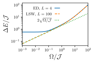
Figure 4: Energy gap of the 2$d$ Heisenberg model as a function of the applied $\Omega$ field: the prediction of LSW theory for a large system ($L=100$) is compared to that of exact diagonalization (ED) for a small system ($L=4$), and to the expected low-field behavior $\Delta E\approx 2{\cal J}\sqrt{\Omega/{\cal J}}$, valid in the thermodynamic limit.

The above Hamiltonian is diagonalized via the Bogoliubov transformation

$$b_{\bm{k}}=u_{\bm{k}}\beta_{\bm{k}}-v_{\bm{k}}\beta^{\dagger}_{-\bm{k}}$$ (9)

into

$${\cal H}=E_{0}+\sum_{\bm{k}}\epsilon_{\bm{k}}\beta_{\bm{k}}^{\dagger}\beta_{\bm{k}}+{\rm const.}$$ (10)

where $\epsilon_{\bm{k}}=\sqrt{A_{\bm{k}}^{2}-B_{\bm{k}}^{2}}$ and

$$u_{\bm{k}}=\frac{1}{\sqrt{2}}\left(\frac{A_{\bm{k}}}{\epsilon_{\bm{k}}}+1\right)^{1/2}~{}~{}~{}v_{\bm{k}}={\rm sign}(B_{\bm{k}})(1-u_{\bm{k}}^{2})^{1/2}~{}.$$ (11)

The observables relevant for the calculation of the squeezing parameter are then

$$\langle J^{x}\rangle = \frac{N}{2}-\frac{1}{2}\sum_{\bm{k}}v_{\bm{k}}^{2}=N-\sum_{\bm{k}}\frac{A_{\bm{k}}}{2\epsilon_{\bm{k}}}$$ (12)

$${\rm Var}(J^{z}) = \frac{N}{4}\left(1+2v_{0}^{2}+u_{0}v_{0}\right)=\frac{N}{4}\sqrt{\frac{A_{0}+B_{0}}{A_{0}-B_{0}}}~{}.$$

The comparison between the predictions of LSW theory and QMC is already shown in the main text, as well as in the next section. Fig. 4 shows the LSW prediction for the spectral gap $\epsilon_{\bm{k}=0}$, compared to the exact diagonalization (ED) for a $N=16$ square lattice, in the case of the SU(2) model with $\Delta=1$. The exact results were obtained via the QuSpin package Weinberg and Bukov (2017, 2019). We observe that the gap predicted by LSW theory is very accurate at large fields; the deviation from the ED results at lower field is due to the saturation of the ED gap to a value $\sim{\cal O}(N^{-1})$ due to the finite size, while the LSW gap closes as $\Omega^{1/2}$ when $\Omega\to 0$.

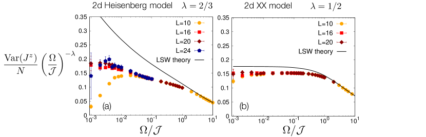
Figure 5: Variance of the squeezed collective-spin component ${\rm Var}(J^{z})$ as a function of the applied field for (a) the 2$d$ Heisenberg model and (b) the 2$d$ XX model. The symbols are QMC data, and the solid line corresponds to LSW theory. The variance is multiplied by the factor $(\Omega/{\cal J})^{\lambda}$ so as to single out its power-law vanishing behavior as $\Omega\to 0$.

II Beyond-spin-wave behavior of spin squeezing in the 2d Heisenberg model

Here we discuss in more details the field scaling of the variance of the squeezed spin component, ${\rm Var}(J^{z})$, in the 2$d$ Heisenberg model and in the 2$d$ XX model. Fig. 5 shows the field dependence of ${\rm Var}(J^{z})$ multiplied by a factor $(\Omega/{\cal J})^{-\lambda}$. A $\lambda$ exponent which leads to a field-independent product corresponds to the field-scaling exponent of ${\rm Var}(J^{z})$ at low fields. While LSW theory predicts $\lambda=1/2$, we clearly observe that this exponent is inadequate for the low-field behavior of the 2$d$ Heisenberg model – see Fig. 5(a). Instead the heuristic choice $\lambda=2/3$ seems to be more appropriate, and we retain this as the low-field scaling of ${\rm Var}(J^{z})$, clearly faster than the LSW prediction. This picture is to be contrasted with that of the 2d XX model – see Fig. 5(b) – for which the low-field scaling of ${\rm Var}(J^{z})$ is captured very well by the LSW prediction (within a $\sim 10\%$ accuracy).

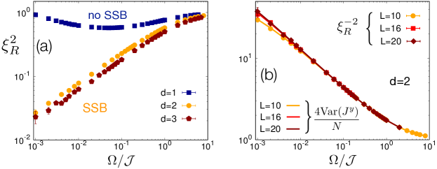
Figure 6: Adiabatic squeezing in the $d$-dimensional XX model. (a) Spin squeezing parameter for various dimensions from QMC simulations: $\xi_{R}^{2}$ is found to scale to zero as $\sqrt{\Omega}$ in the presence of spontaneous symmetry breaking (SSB) in the ground state for $d=2$ and 3, while it does not vanish in its absence ($d=1$). (b) Comparison between the inverse spin squeezing parameter $\xi_{R}^{-2}$ and $4{\rm Var}(J^{y})/N$ for the 2$d$ XX model for various system sizes. The coincidence of the two quantities shows that the ground state of the system is a minimal-uncertainty quantum state for all the field values we explored.

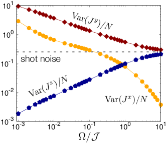
Figure 7: Variance of the three components of the collective spin in the ground state of the 2$d$ Heisenberg model (QMC data for a $L=20$ lattice). The dashed line marks the shot-noise limit ${\rm Var}(J^{\alpha})/N=1/4$.

III QMC results for the XX model

In this section we show our results for the XX model ($\Delta=0$), relevant e.g. for the physics of superconducting circuits Mi et al. (2021) as well of ultracold spinful atoms in optical lattices Jepsen et al. (2020). Fig. 6(a) shows the field scaling of the spin squeezing parameter for the models in $d=1,2$ and 3 dimensions. Similarly to the case of the Heisenberg model discussed in the main text, the scaling of the spin squeezing parameter as $\xi_{R}^{2}\sim\Omega^{1/2}$ is observed in $d=2,3$, while it is absent in $d=1$ because of the lack of spontaneous symmetry breaking.

Fig. 6(b) also shows that for $d=2$ the ground state at finite $\Omega$ is a state of minimal spin uncertainty, for which $\xi^{-2}_{R}\approx 4{\rm Var}(J^{y})/N$. Similar result is also found in $d=3$.

IV Ground-state variance of the collective spin components

In Fig. 7 we compare the variance of the three spin components $J^{x}$, $J^{y}$ and $J^{z}$ in the ground state of the 2$d$ Heisenberg model in a finite $\Omega$ field. We clearly observe that ${\rm Var}(J^{y})$ is the largest among the three, meaning that the highest sensitivity of the state to rotations is achieved when the rotation axis is the $y$ axis. Also, among all operators of the form $O=\sum_{i}o_{i}$ (with $o_{i}$ a local operator associated to a finite neighborhood of site $i$) $J^{y}=\sum_{i}S_{i}^{y}$ is arguably the one that has the largest variance: this can be deduced from the fact that the variance is the integral of the correlation function ${\rm Var}(O)=\sum_{ij}\langle o_{i}o_{j}\rangle-\langle o_{i}\rangle\langle o_{j}\rangle$, and the correlation function which has the slowest spatial decay, leading to the largest integral, is the one of the order parameter in the SSB mechanism, corresponding to any spin component in the xy plane in the limit $\Omega\to 0$.

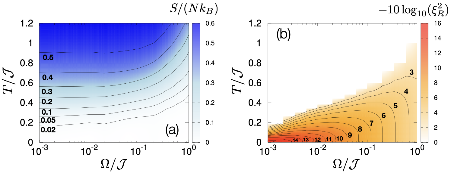
Figure 8: Entropy and squeezing maps for the 2$d$ Heisenberg model. (a) Entropy map in the $(\Omega/{\cal J},T/{\cal J})$ plane; (b) squeezing map in the $(\Omega/{\cal J},T/{\cal J})$ plane. All the QMC data shown here were obtained for a $L=24$ lattice.

V Adiabatic squeezing at finite entropy

Entropy curves can be obtained via QMC using a simple scheme of linear interpolation on the energy data. A direct result of the QMC calculation is the average energy per spin $e(T)=\langle\cal H\rangle/N$. From a sufficiently fine grid $\{T_{k}\}$ of temperature values, we can then reconstruct the $e(T)$ curve by linear interpolation between two successive temperatures $e(T_{k})$ and $e(T_{k+1})$, and therefore obtain the specific heat at the mid-point temperature $T_{k+1/2}=(T_{k+1}+T_{k})/2$ as

$$c(T_{k+1/2})\approx\frac{e(T_{k+1})-e(T_{k})}{T_{k+1}-T_{k}}~{}.$$ (13)

In order to obtain the $s(T)=S(T)/(Nk_{B})$ curve via integration of the specific-heat data, we can proceed by a linear interpolation of the specific heat between midpoints

$$c(T)\approx c(T_{k+1/2})+\frac{c(T_{k+3/2})-c(T_{k+1/2})}{T_{k+3/2}-T_{k+1/2}}(T-T_{k+1/2})$$ (14)

valid for $T_{k+1/2}\leq T\leq T_{k+3/2}$. This then allows us to estimate the entropy increment between two temperatures of the grid $\{T_{k}\}$ as

$$\Delta s_{k}=s(T_{k+1})-s(T_{k})=\delta s_{k,<}+\delta s_{k,>}$$ (15)

where

$$\begin{split}&\delta s_{k,<}=\int_{T_{k}}^{T_{k+1/2}}dT~{}\frac{c(T)}{T}\\ &\approx\left[c(T_{k-1/2})-\frac{c(T_{k+1/2})-c(T_{k-1/2})}{T_{k+1/2}-T_{k-1/2}}\right]\log\left(\frac{T_{k+1/2}}{T_{k}}\right)\\ &+\frac{c(T_{k+1/2})-c(T_{k-1/2})}{T_{k+1/2}-T_{k-1/2}}(T_{k+1/2}-T_{k})\end{split}$$ (16)

and

$$\begin{split}&\delta s_{k,>}=\int_{T_{k+1/2}}^{T_{k+1}}dT~{}\frac{c(T)}{T}\\ &\approx\left[c(T_{k+1/2})-\frac{c(T_{k+3/2})-c(T_{k+1/2})}{T_{k+3/2}-T_{k+1/2}}\right]\log\left(\frac{T_{k+1}}{T_{k+1/2}}\right)\\ &+\frac{c(T_{k+3/2})-c(T_{k+1/2})}{T_{k+3/2}-T_{k+1/2}}(T_{k+1}-T_{k+1/2})~{}.\end{split}$$ (17)

We have verified that this entropy reconstruction scheme delivers a similar result as that of a high-order polynomial fit of the $e(T)$ curve, as used e.g. in Ref. Carcy et al. (2021); yet it has the advantage that no fitting procedure is involved.

Fig. 8(a) shows the resulting entropy map for the 2$d$ Heisenberg model as a function of temperature and applied field. We then combine the entropy map with the squeezing map at finite temperatures shown in Fig. 8(b), to reconstruct the squeezing dependence on field and entropy, reported in Fig. 3 of the main text.

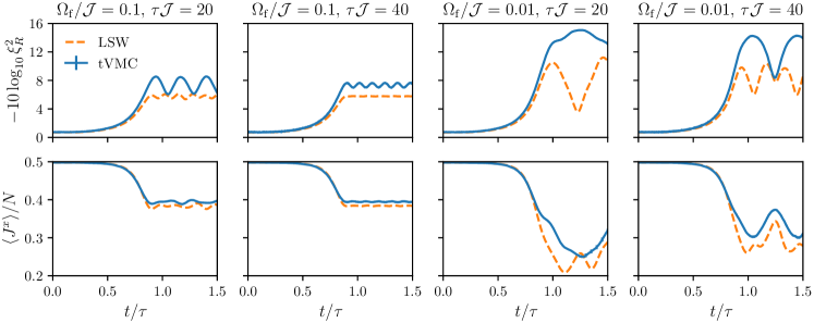
Figure 9: Comparison between tVMC and LSW results for the evolution of the squeezing parameter $\xi_{R}^{2}$ (upper row) and of the magnetization per spin $\langle J^{x}\rangle/N$ (lower row) along quasi-adiabatic ramps starting from the ground state at $\Omega_{\rm i}=10{\cal J}$ and ending at two different values $\Omega_{\rm f}=0.1{\cal J}$ and $0.01{\cal J}$, with two different ramp durations, $\tau{\cal J}=20$ and 40.

VI Time-dependent spin-wave theory vs. time-dependent variational Monte Carlo

In order to corroborate the results coming from time-dependent variational Monte Carlo (tVMC), shown in the main text, we have compared them with an independent calculation, based on time-dependent LSW theory. This comparison is interesting especially at high $\Omega$ fields, for which, as we have seen in the main text and in the results above, the predictions of (static) LSW theory are fully quantitative.

As in the main text, we consider an evolution which starts from the ground state at an initial field $\Omega_{\rm i}=10{\cal J}$, and ends at a final value $\Omega_{\rm f}$ with schedule $\Omega(t)=\Omega_{\rm i}+F(t/\tau)(\Omega_{\rm f}-\Omega_{\rm i})$, where $F(x)$ is reported in the main text. The time dependence of the field $\Omega(t)$ translates into a time-dependent $A_{\bm{k}}(t)$ parameter entering in the linear bosonic Hamiltonian Eq. (5). The evolution of the Gaussian state of the bosonic variables within LSW is fully described by the two correlation functions $G_{\bm{k}}=\langle b_{\bm{k}}^{\dagger}b_{\bm{k}}\rangle$ and $F_{\bm{k}}=\langle b_{\bm{k}}b_{-\bm{k}}\rangle$, which evolve according to the equations (descending from the Heisenberg equations for the $b_{\bm{k}}$ operators):

$$\frac{dG_{\bm{k}}}{dt} = -2~{}(1+\delta_{\bm{k},0})~{}B_{\bm{k}}~{}{\rm Im}(F_{\bm{k}})$$ (18)

$$\frac{dF_{\bm{k}}}{dt} = -i(1+\delta_{\bm{k},0})\left[2A_{\bm{k}}(t)F_{\bm{k}}+B_{\bm{k}}(1+G_{\bm{k}}+G_{-\bm{k}})\right]$$

and from which our main observables of interest can be deduced

$$\langle J^{x}\rangle = \frac{N}{2}-\sum_{\bm{k}}G_{\bm{k}}$$

$${\rm Var}(J^{z}) = \frac{1}{4}\left[1+G_{\bm{k}}+G_{-\bm{k}}+2{\rm Re}(F_{\bm{k}})\right]~{}.$$ (19)

Fig. 9(a)-(b) shows the comparison between the results of tVMC and those of LSW theory, obtained for the 2$d$ Heisenberg model with $L=12$, for final fields $\Omega_{f}=0.1{\cal J}$ and $0.01{\cal J}$ and ramp durations $\tau{\cal J}=20,40$ (same as those shown in Fig. 3 in the main text). In particular we show the evolution of the spin squeezing parameter $\xi_{R}^{2}$ and of the magnetization per spin $\langle J^{x}\rangle/N$. We observe that tVMC and LSW agree perfectly for most of the ramp duration, while they deviate upon approaching the end of the ramp ($t=\tau$) and in the subsequent time evolution, during which $\Omega$ is held fixed at its final value. This deviation is easily understood within an adiabatic picture, namely from the fact that (static) LSW theory overestimates the $\xi_{R}^{2}$ parameter (as shown in the main text), namely it underestimates $-10\log_{10}(\xi_{R}^{2})$ shown in the figure; while the tVMC results for quasi-adiabatic ramps produce values of the $\xi_{R}^{2}$ which are systematically closer to the (static) QMC estimate. From this comparison we conclude therefore that our tVMC results, while not numerically exact, are fully quantitative, as they reproduce the LSW results at large fields ($t<\tau$); and, for quasi-adiabatic ramps, they oscillate around a value compatible with the QMC prediction for $t>\tau$.

References

- Preskill (2012) J. Preskill, Quantum computing and the entanglement frontier (2012), eprint 1203.5813.
- Kaufman et al. (2016) A. M. Kaufman, M. E. Tai, A. Lukin, M. Rispoli, R. Schittko, P. M. Preiss, and M. Greiner, Science 353, 794 (2016).
- Georgescu et al. (2014) I. M. Georgescu, S. Ashhab, and F. Nori, Rev. Mod. Phys. 86, 153 (2014), URL https://link.aps.org/doi/10.1103/RevModPhys.86.153.
- Nielsen and Chuang (2000) M. A. Nielsen and I. L. Chuang, Quantum Computation and Quantum Information (Cambridge University Press, 2000), ISBN 9780521635035.
- Gühne and Tóth (2009) O. Gühne and G. Tóth, Physics Reports 474, 1 (2009), ISSN 0370-1573, URL https://www.sciencedirect.com/science/article/pii/S0370157309000623.
- Wineland et al. (1994) D. J. Wineland, J. J. Bollinger, W. M. Itano, and D. J. Heinzen, Phys. Rev. A 50, 67 (1994), URL https://link.aps.org/doi/10.1103/PhysRevA.50.67.
- Sørensen et al. (2001) A. Sørensen, L.-M. Duan, J. I. Cirac, and P. Zoller, Nature 409, 63 (2001), URL https://doi.org/10.1038/35051038.
- Pezzè et al. (2018) L. Pezzè, A. Smerzi, M. K. Oberthaler, R. Schmied, and P. Treutlein, Rev. Mod. Phys. 90, 035005 (2018), URL https://link.aps.org/doi/10.1103/RevModPhys.90.035005.
- Louchet-Chauvet et al. (2010) A. Louchet-Chauvet, J. Appel, J. J. Renema, D. Oblak, N. Kjaergaard, and E. S. Polzik, New Journal of Physics 12, 065032 (2010), URL https://doi.org/10.1088/1367-2630/12/6/065032.
- Leroux et al. (2010a) I. D. Leroux, M. H. Schleier-Smith, and V. Vuletić, Phys. Rev. Lett. 104, 250801 (2010a), URL https://link.aps.org/doi/10.1103/PhysRevLett.104.250801.
- Pedrozo-Peñafiel et al. (2020) E. Pedrozo-Peñafiel, S. Colombo, C. Shu, A. F. Adiyatullin, Z. Li, E. Mendez, B. Braverman, A. Kawasaki, D. Akamatsu, Y. Xiao, et al., Nature 588, 414 (2020), ISSN 1476-4687, URL https://doi.org/10.1038/s41586-020-3006-1.
- Schulte et al. (2020) M. Schulte, C. Lisdat, P. O. Schmidt, U. Sterr, and K. Hammerer, Nature Communications 11, 5955 (2020), ISSN 2041-1723, URL https://doi.org/10.1038/s41467-020-19403-7.
- Muessel et al. (2014) W. Muessel, H. Strobel, D. Linnemann, D. B. Hume, and M. K. Oberthaler, Phys. Rev. Lett. 113, 103004 (2014), URL https://link.aps.org/doi/10.1103/PhysRevLett.113.103004.
- Salvi et al. (2018) L. Salvi, N. Poli, V. Vuletić, and G. M. Tino, Phys. Rev. Lett. 120, 033601 (2018), URL https://link.aps.org/doi/10.1103/PhysRevLett.120.033601.
- Shankar et al. (2019) A. Shankar, L. Salvi, M. L. Chiofalo, N. Poli, and M. J. Holland, 4, 045010 (2019), URL https://doi.org/10.1088/2058-9565/ab455d.
- Ma et al. (2011) J. Ma, X. Wang, C. Sun, and F. Nori, Phys. Rep. 509, 89 (2011), ISSN 0370-1573, URL http://www.sciencedirect.com/science/article/pii/S0370157311002201.
- Kitagawa and Ueda (1993) M. Kitagawa and M. Ueda, Phys. Rev. A 47, 5138 (1993), URL https://link.aps.org/doi/10.1103/PhysRevA.47.5138.
- Estève et al. (2008) J. Estève, C. Gross, A. Weller, S. Giovanazzi, and M. K. Oberthaler, Nature 455, 1216 (2008), URL https://doi.org/10.1038/nature07332.
- Riedel et al. (2010) M. F. Riedel, P. Böhi, Y. Li, T. W. Hänsch, A. Sinatra, and P. Treutlein, Nature 464, 1170 (2010), URL https://doi.org/10.1038/nature08988.
- Bohnet et al. (2016) J. G. Bohnet, B. C. Sawyer, J. W. Britton, M. L. Wall, A. M. Rey, M. Foss-Feig, and J. J. Bollinger, Science 352, 1297 (2016), URL https://doi.org/10.1126/science.aad9958.
- Leroux et al. (2010b) I. D. Leroux, M. H. Schleier-Smith, and V. Vuletić, Phys. Rev. Lett. 104, 073602 (2010b), URL https://link.aps.org/doi/10.1103/PhysRevLett.104.073602.
- Hosten et al. (2016) O. Hosten, N. J. Engelsen, R. Krishnakumar, and M. A. Kasevich, Nature 529, 505 (2016), URL https://doi.org/10.1038/nature16176.
- Frérot and Roscilde (2018) I. Frérot and T. Roscilde, Phys. Rev. Lett. 121, 020402 (2018), URL https://link.aps.org/doi/10.1103/PhysRevLett.121.020402.
- Anderson (1997) P. W. Anderson, Basic Notions of Condensed Matter Physics (Taylor & Francis, Boca Raton (FL), 1997).
- Tasaki (2018) H. Tasaki, J. Stat. Phys. 174, 735 (2018), URL https://doi.org/10.1007/s10955-018-2193-8.
- Beekman et al. (2019) A. J. Beekman, L. Rademaker, and J. van Wezel, SciPost Phys. Lect. Notes p. 11 (2019), URL https://scipost.org/10.21468/SciPostPhysLectNotes.11.
- Comparin et al. (2021) T. Comparin, F. Mezzacapo, and T. Roscilde, Universal spin squeezing from the tower of states of -symmetric spin hamiltonians (2021), eprint 2103.07354.
- Facon et al. (2016) A. Facon, E.-K. Dietsche, D. Grosso, S. Haroche, J.-M. Raimond, M. Brune, and S. Gleyzes, Nature 535, 262 (2016), ISSN 1476-4687, URL https://doi.org/10.1038/nature18327.
- Takamoto et al. (2005) M. Takamoto, F.-L. Hong, R. Higashi, and H. Katori, Nature 435, 321 (2005), ISSN 1476-4687, URL https://doi.org/10.1038/nature03541.
- Campbell et al. (2017) S. L. Campbell, R. B. Hutson, G. E. Marti, A. Goban, N. D. Oppong, R. L. McNally, L. Sonderhouse, J. M. Robinson, W. Zhang, B. J. Bloom, et al., Science 358, 90 (2017).
- Duan et al. (2003) L.-M. Duan, E. Demler, and M. D. Lukin, Phys. Rev. Lett. 91, 090402 (2003), URL https://link.aps.org/doi/10.1103/PhysRevLett.91.090402.
- Jepsen et al. (2020) P. N. Jepsen, J. Amato-Grill, I. Dimitrova, W. W. Ho, E. Demler, and W. Ketterle, Nature 588, 403 (2020), URL https://doi.org/10.1038/s41586-020-3033-y.
- Sun et al. (2021) H. Sun, B. Yang, H.-Y. Wang, Z.-Y. Zhou, G.-X. Su, H.-N. Dai, Z.-S. Yuan, and J.-W. Pan, Nature Physics 17, 990 (2021), ISSN 1745-2481, URL https://doi.org/10.1038/s41567-021-01277-1.
- Greif et al. (2013) D. Greif, T. Uehlinger, G. Jotzu, L. Tarruell, and T. Esslinger, Science 340, 1307 (2013), eprint https://www.science.org/doi/pdf/10.1126/science.1236362, URL https://www.science.org/doi/abs/10.1126/science.1236362.
- Mazurenko et al. (2017) A. Mazurenko, C. S. Chiu, G. Ji, M. F. Parsons, M. Kanász-Nagy, R. Schmidt, F. Grusdt, E. Demler, D. Greif, and M. Greiner, Nature 545, 462 (2017), URL https://doi.org/10.1038/nature22362.
- Syljuåsen and Sandvik (2002) O. F. Syljuåsen and A. W. Sandvik, Phys. Rev. E 66, 046701 (2002), URL http://link.aps.org/doi/10.1103/PhysRevE.66.046701.
- Thibaut et al. (2019) J. Thibaut, T. Roscilde, and F. Mezzacapo, Phys. Rev. B 100, 155148 (2019), URL https://link.aps.org/doi/10.1103/PhysRevB.100.155148.
- (38) See Supplemental Material (SM) for a discussion of: 1) Spin-wave theory of the XXZ model; 2) beyond LSW effects in the squeezing of in the 2 Heisenberg model; 3) QMC results for squeezing in the 2 XX model; 4) the field dependence of the variance of all spins components in the 2 Heisenberg model; 5) details on the calculation of squeezing at finite temperature/entropy; and 6) comparison between tVMC and LSW results for the evolution along quasi-adiabatic ramps.
- Manousakis (1991) E. Manousakis, Rev. Mod. Phys. 63, 1 (1991), URL https://link.aps.org/doi/10.1103/RevModPhys.63.1.
- Roscilde et al. (2021) T. Roscilde, F. Mezzacapo, and T. Comparin, Phys. Rev. A 104, L040601 (2021), URL https://link.aps.org/doi/10.1103/PhysRevA.104.L040601.
- Auerbach (1994) A. Auerbach, Interacting electrons and quantum magnetism (Springer, New York, 1994).
- Albash and Lidar (2018) T. Albash and D. A. Lidar, Rev. Mod. Phys. 90, 015002 (2018), URL https://link.aps.org/doi/10.1103/RevModPhys.90.015002.
- Mi et al. (2021) X. Mi, P. Roushan, C. Quintana, S. Mandra, J. Marshall, C. Neill, F. Arute, K. Arya, J. Atalaya, R. Babbush, et al., Information scrambling in computationally complex quantum circuits (2021), eprint 2101.08870.
- Browaeys and Lahaye (2020) A. Browaeys and T. Lahaye, Nat. Phys. 16, 132 (2020), URL https://doi.org/10.1038/s41567-019-0733-z.
- Brydges et al. (2019) T. Brydges, A. Elben, P. Jurcevic, B. Vermersch, C. Maier, B. P. Lanyon, P. Zoller, R. Blatt, and C. F. Roos, Science 364, 260 (2019), URL https://doi.org/10.1126/science.aau4963.
- Weinberg and Bukov (2017) P. Weinberg and M. Bukov, SciPost Phys. 2, 003 (2017), URL https://scipost.org/10.21468/SciPostPhys.2.1.003.
- Weinberg and Bukov (2019) P. Weinberg and M. Bukov, SciPost Phys. 7, 20 (2019), URL https://scipost.org/10.21468/SciPostPhys.7.2.020.
- Carcy et al. (2021) C. Carcy, G. Hercé, A. Tenart, T. Roscilde, and D. Clément, Phys. Rev. Lett. 126, 045301 (2021), URL https://link.aps.org/doi/10.1103/PhysRevLett.126.045301.