Localization and delocalization properties in quasi-periodically driven one-dimensional disordered system

Abstract

Localization and delocalization of quantum diffusion in time-continuous one-dimensional Anderson model perturbed by the quasi-periodic harmonic oscillations of $M$ colors is investigated systematically, which has been partly reported by the preliminary letter [PRE 103, L040202(2021)]. We investigate in detail the localization-delocalization characteristics of the model with respect to three parameters: the disorder strength $W$, the perturbation strength $\epsilon$ and the number of the colors $M$ which plays the similar role of spatial dimension. In particular, attentions are focused on the presence of localization-delocalization transition (LDT) and its critical properties. For $M\geq 3$ the LDT exists and a normal diffusion is recovered above a critical strength $\epsilon$, and the characteristics of diffusion dynamics mimic the diffusion process predicted for the stochastically perturbed Anderson model even though $M$ is not large. These results are compared with the results of time-discrete quantum maps, ie., Anderson map and the standard map. Further, the features of delocalized dynamics is discussed in comparison with a limit model which has no static disordered part.

I Introduction

It has been theoretically and experimentally shown that the three-dimensional random system undergoes an Anderson transition (AT) from insulator to metallic conductor due to decrease in the potential disorder anderson58 ; ishii73 ; lifshiz88 ; abrahams10 . Furthermore, in recent numerical experiments, the properties of AT in 4-dimensional and 5-dimensional random systems have been also studied markos06 ; garcia07 ; slevin14 ; tarquini17 . In the system with the AT, a localization-delocalization transition (LDT) can exist, and its existence can be directly observed by the wavepacket dynamics of initially localized wave packet, where the delocalization is observed as an appearance of normal diffusion.

In higher-dimensional Anderson model the appearance of delocalized states is quite natural, and it is expected that the self-consistent mean-field theory works well in such systems vollhard80 ; wolfle10 . However, even in higher-dimensional Anderson models the deviation of the critical value and the critical exponent predicted by the SCT was recently reported by using the properties of the energy spectrum tarquini17 .

The relationship between the dimension of the Anderson model and the characteristics of the LDT is an interesting problem from a different point of view. Increase of the system’s dimension $d$ may be performed in a quite different way: an alternative way to increase $d$ is to make the system interact with many dynamical degrees of freedom. Indeed, even in the one-dimensional (1D) Anderson model exhibiting a strong exponential localization, the localization is released and normal diffusion is induced by the application of arbitrarily small stochastic perturbation, which can be considered as a superposition of an infinite number of incommensurate harmonic degrees of freedoms haken72 ; palenberg00 ; moix13 ; knap17 . This can be considered as a limiting example of delocalization realized in systems with infinite degrees of freedom.

Then it is a quite natural question to inquire how the number of the degrees of harmonic modes $M$ controlls the localization and delocalization in disordered systems. (The harmonic modes may be replaced the active phonon modes.) Indeed, in the case of chaotic quantum maps such as the standard map (SM), the harmonic perturbation destroys the dynamical localization and restores the chaotic diffusion casati89 ; lopez12 ; lopez13 ; yamada15 ; yamada18 ; yamada20 , which is supported by the Maryland transformation asserting the equivalence between the SM and a $M+1$-dimensional lattice with a quasi-periodic disorder.

Quantum maps is a very powerful model which can easily be treated by numerical method because its time is discretized, but it is not a natural system. Instead, as a time-continuous model, we proposed a time-continuous 1D Anderson model interacting with $M$ incommensurate harmonic modes yamada98 ; yamada99 . For $M=1$, the maintenance of localization can be shown by the Floquet theory holhaus95 ; Martinez06 . But for $M\geq 2$, diffusion-like behaviors are observed numerically at least on a finite time scale if the perturbation strength is strong enough. In this system, the $M-$modes can be treated as a quantum dynamical degrees of freedom, and so the whole system can be regarded as an autonomous quantum dynamical system with $(M+1)-$degrees of freedom. There has been some studies showing strong localized property of the dynamics for the same type of harmonically perturbed models. It is inferred from analytical calculation and rigorous proofs that the localization persists against the dynamical perturbation consisting of finite number of the modes hatami16 ; wang04 . In particular, the persistence of the localization for $1\leq M<\infty$ is mathematically claimed in the regime of weak enough dynamical perturbations and strong disorder potential wang04 . On the other hand, as mentioned above, a stochastic perturbation which corresponds to $M\to\infty$ can restore a complete diffusion. The presence of the LDT in harmonically perturbed 1D Anderson model has not been yet clarified.

In our preliminary report it was shown that if there exist three or more harmonics ($M\geq 3$), the LDT occurs with the increase of the perturbation strength and the Anderson localized states can be delocalized yamada21 . This work is a full report of the localization-delocalization characteristics of the 1D Anderson model perturbed by polychromatic perturbations, which is numerically observed by changing the three parameters: the disorder strength $W$, perturbation strength $\epsilon$ and the number of the modes $M$ of the oscillations. We are particularly interested in making clear how the number $M$ controls the characteristics of LDT. Additionally as a limiting situation of our model mentioned above, we can consider a model system without the static random potential. Such a version leads to a quantum state that models the ultimate limit of delocalization exhibited by our model, which will be discussed in detail.

Since the direct numerical wavepacket propagation of the original continuous-time model is too time consuming, we proposed a discrete-time quantum map version of the original time-continuous model, which we called the Anderson map (AM), and investigated its nature in comparison with the SM and many-dimensional Anderson model yamada15 ; yamada18 ; yamada20 . Comparison of the original time-continuous model with the AM is also a purpose of this article.

Recently realization of ergodic state in isolated quantum systems with many degrees of freedom has been extensively studied gutzwiller91 ; borgonovi97 ; neill16 ; notarnicola18 ; piga19 . As mentioned above, our system is a closed quantum dynamical system with $M+1$ degrees of freedom, and the LDT may be looked upon as a transition to an ergodic state even though $M$ is small. The transition to a delocalized behavior is a “self-organization” of a irreversible relaxation process in quantum systems with a small-number of degrees of freedom stressed in Ref.ikeda93 . With this regard the minimal number of $M$ above which the LDT takes place is a quite interesting problem.

The plan of the present work is as follows. In the next section, the models used in the present paper are introduced. In Sec.III, the characteristics of the localization phase which is dominant when the number $M$ is small ie., $M=0,1,2$ are explored. A hypothesis due to the intrinsic nature of time-continuous model, which was not taken into account in our preliminary report yamada21 , is discussed. It is used as a base of the following analysis. Next, in Sec.IV, the presence of LDT for the case of $M\geq 3$ is demonstrated and the characteristic of the LDT are clarified on the basis of the one-parameter scaling theory together with the above hypothesis. The presence of critical subdiffusion, invariant nature of critical perturbation strength and their dependency upon $M$ are fully discussed. After these arguments, we reexamine the absence of LDT in the case of $M=2$ in Sec.V. Finally, in Sec.VI, characteristic of the normal diffusion in the delocalized states is discussed in some detail. Summary and discussion are devoted in the last section.

II Models

We consider one-dimensional tightly binding disordered system represented by the lattece site basis $|n\rangle$(n:integer) with the probability amplitude $\Psi_{n}$, which is driven by time-dependent quasi-periodic perturbation. The Schrödinger equation of the above system is represented by

$$i\hbar\frac{\partial\Psi_{n}(t)}{\partial t}=\Psi_{n-1}(t)+\Psi_{n+1}(t)+V(n,t)\Psi_{n}(t),$$ (1)

where $V(n,t)$ is the time dependent on-site potential. We deal with the following two cases, $V_{A}(n,t)$ and $V_{B}(n,t)$, as $V(n,t)$ with coherent periodic perturbation $f_{\epsilon}(t)$:

$$V(n,t)=\begin{cases}V_{A}(n,t)=V(n)[1+f_{\epsilon}(t)]&({\rm A-model})\\ V_{B}(n,t)=V(n)f_{\epsilon}(t)&({\rm B-model}).\end{cases}$$ (2)

The coherent periodic perturbation $f_{\epsilon}(t)$ is given as,

$$f_{\epsilon}(t)=\frac{\epsilon}{\sqrt{M}}\sum_{i}^{M}\cos(\omega_{i}t+\theta_{i}),$$ (3)

where $M$ and $\epsilon$ are number of the frequency component and the relative strength of the perturbation, respectively. Note that the long-time average of the total power of the perturbation is normalized to $\overline{f_{\epsilon}(t)^{2}}=\epsilon^{2}/2$. The frequencies $\{\omega_{i}\}(i=1,...,M)$ are taken as mutually incommensurate numbers of order $O(1)$ given in Appendix A. Here we take $\theta_{i}=0$($i=1,2,...M$) to see long-term results that do not depend on the details of initial phases $\{\theta_{i}\}$. The static on-site disorder potential is represented as $V(n)=Wv_{n}$. $W$ denotes the strength of potential, and $v_{n}$ is uniform random variable with the range $[-1,1]$ which is decorrelatd between different sites. In the A-model, it becomes the Anderson model if we take $\epsilon=0$, and the Anderson localization occurs. How the localization may become delocalized by increasing the perturbation strength $\epsilon$ is the main problem to be clarified. On the other hand, the B-model is controlled by the combined parameter $\epsilon W$, and if we take $\epsilon W=0$, the eigenstates are the Bloch states. The issue is how the ballistic motion of $\epsilon=0$ may make transition to a stochastic motion such as the normal diffusion by increasing $\epsilon$, which models stochastization of ballistic electrons by dynamical impurities.

We remark that time-dependent model (1) has an autonomous representation. The isolated harmonic modes form a $M-$dimensional ladder of the eigenstate $|\{n_{i}\}\rangle$ which is assigned by the set of integers $\{n_{i}\}~{}(1\leq i\leq M)$ as the quantum numbers and has the energy $E_{h}(\{n_{i}\}):=\sum_{i=1}^{M}\omega_{i}n_{i}$. If we denote the eigenstate of 1D Anderson model of $\epsilon=0$ by $|N\rangle$, which are the Anderson localized state (A-model) or Bloch states (B-model) having the energy eigenvalue $E_{N}$, then Eq. (1) is equivalent to the autonomous Schrödinger equation describing the transition process among $(M+1)-$dimensional lattice of sites assigned by $(N,\{n_{i}\})$: let the probability amplitude of the quantum state $|N,\{n_{i}\}\rangle=|N\rangle|\{n_{i}\}\rangle$ be $\Phi(N,\{n_{i}\})$, then the Schrödinger equation is represented by

$$i\hbar\frac{d\Phi(N,\{n_{i}\})}{dt}=\left[E_{N}+E_{h}(\{n_{i}\})\right]\Phi(N,\{n_{i}\})$$

$$+\frac{\epsilon}{\sqrt{M}}\sum_{N^{\prime}}\sum_{j=1}^{M}W_{NN^{\prime}}\Phi(N^{\prime},n_{1},..,n_{j}\pm 1,n_{j+1}...n_{M}),$$ (4)

where $W_{NN^{\prime}}$ is the transition element $W\sum_{n}\langle N|n\rangle v_{n}\langle n|N^{\prime}\rangle$ and $\{|n\rangle\}$ is an orthonormalized basis set representing the lattice site $n$. The equivalent of Eq.(II) to the autonomous version of Eq(1) is presented in Appendix B.

We basically limit the perturbation strength to $\epsilon<0.3$, since we are interested in how small $\epsilon$ may destroy the localization effect. As $\epsilon$ increases far beyond the perturbation regime, the A-model will gradually approach to the B-model.

As the tool of numerical integration of Eq.(1), we use the second-order symplectic integrator

$$U(\ell)={\rm e}^{-i\Delta t\cos(n)/2\hbar}{\rm e}^{-iV(n,\ell\Delta t)/\hbar}{\rm e}^{-i\Delta t\cos(n)/2\hbar}$$ (5)

with the small-enough time step $\Delta t=0.02\sim 0.05$, where the value of Planck constant is taken $\hbar=1/8$. The system and ensemble sizes are $2^{15}-2^{16}$ and $10-50$, respectively, throughout this paper. We use a localized state at $n=n_{0}$ as the initial state and numerically observe the spread of the wavepacket measured by the mean square displacement (MSD),

$$m_{2}(t)=\sum_{n}(n-n_{0})^{2}\langle|\Psi(n,t)|^{2}\rangle.$$ (6)

In the limit $M\to\infty$, the quasiperiodic perturbation $f_{\epsilon}(t)$ can be identified with the delta-correlated stochastic force $n(t)$ characterized by $\langle n(t)n(t^{`})\rangle=\epsilon_{s}^{2}\delta(t-t^{`})$ with the strength $\epsilon_{s}$. In this paper, corresponding to A-model and B-model, we consider the stochastic version of the two models in which the harmonic force $f_{\epsilon}(t)$ is replaced by the noise force $n(t)=\epsilon_{s}n_{1}(t)$, which varies at random in time uniformly in the range $[-1,1]$:

$$\begin{cases}V_{SA}(n,t)=V(n)[1+\epsilon_{s}n_{1}(t)]&({\rm SA-model})\\ V_{SB}(n,t)=V(n)\epsilon_{s}n_{1}(t)&({\rm SB-model}),\end{cases}$$ (7)

We call these SA-model and SB-model, respectively. In the SA-model, the localization is destroyed by the stochastic perturbation and the normal diffusion $m_{2}(t)=Dt$ with the diffusion constant $D$ appears for $t\to\infty$ yamada98 ; yamada99 , as was first pointed out by Haken and his coworkers haken72 ; palenberg00 . They predicted analytically the diffusion constant $D$ for the white Gaussian noise as

$$D=\lim_{t\to\infty}\dfrac{m_{2}(t)}{t}\propto\frac{\epsilon_{s}^{2}}{\epsilon_{s}^{4}+W^{2}/3}.$$ (8)

for weak enough $\epsilon_{s}$. The diffusion constant increases as $D\propto\epsilon_{s}^{2}$ for $\epsilon_{s}<<1$ and it reaches maximum at $\epsilon_{s}^{*}=\frac{W}{\sqrt{3}}$, and it finally decreases as $D\propto\epsilon_{s}^{-2}$. The noise-induced diffusion has been extended for a random lattice driven by the colored noise, including the hopping disorder effect moix13 ; knap17 .

For finite $M$, $f_{\epsilon}(t)$ can no longer be replaced by the random noise, and it playes as a coherent dynamical perturbation, and the system corresponds to a quantum dynamical system with $(M+1)$-degrees of freedom.

III Localized states of A-model

First of all we show in this section the localization characteristics exhibited by our model Eq.(1). The cases of $M=1,2$ are particularly focused on, and a basic hypothesis to interpret all our numerical results is discussed in connection with the localization characteristics of our system.

III.1 dynamics toward localization; localizing evolution

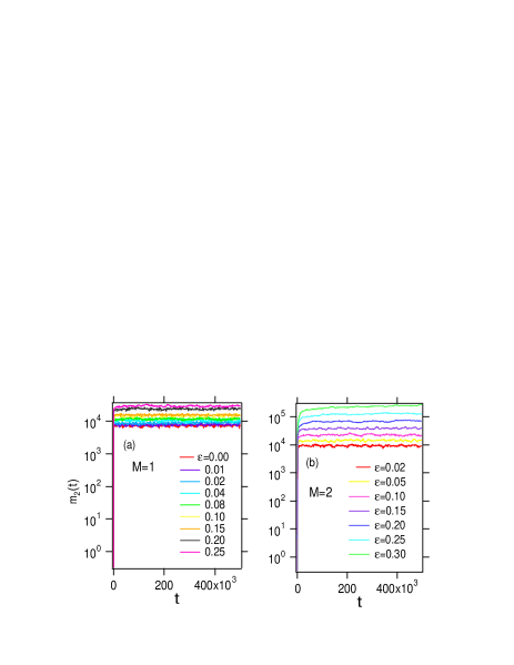
Figure 1: (Color online) The plots of $m_{2}(t)$ as a function of time for different values of $\epsilon$ increasing from bottom to top in the perturbed Anderson model. (a)$M=1$, $W=1.0$. (b)$M=2$, $W=1.0$. Note that the horizontal axes are in the logarithmic scale.

Figure 1(a) shows the time-dependence of MSD for some typical cases of the monochromatically perturbed A-model, for which the growth of time-dependence is saturated at a certain level. The the spread of the wavepacket becomes larger as the perturbation strength increases. This is the same tendency as was observed for the Anderson map. In this paper, we directly compute the localization length (LL) by

$$\xi_{M}=\sqrt{m_{2}(\infty)},$$ (9)

where $m_{2}(\infty)$ indicates the numerically saturated MSD reached after a sufficiently long time evolution. For $M=1$ the localization is manifest. Even in the case of $M=2$, localization occurs and the LL increases as the perturbation strength increases , as can be seen from the Fig.1(b).

Application of harmonic perturbation in general enhances the LL. The enhancement of LL is conspicuous for $M=2$, and the numerical evaluation of $\xi_{M}$ directly from the long time behavior of MSD is possible only in the limited range of $\epsilon<0.4$.

III.2 $W-$dependence of localization length

Figure 2 shows $W-$dependence of the LL $\xi_{M}$ for $M=0,1,2$. In all cases, it is naturally found that for $\epsilon<<1$ the larger $W$, the stronger the localization is, and the LL follows the rule

$$\xi_{M}\sim\frac{A_{M}(\epsilon)}{W^{2}},$$ (10)

where $A_{M}(\epsilon)$ depends on $M$ and $\epsilon$. The $W^{-2}-$dependence of the LL has been commonly observed in the case of quantum map systems yamada20 . For $M=1$ the persistence of localization can be expected as is argued in Appendix C.

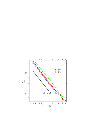
Figure 2: (Color online) Localization length $\xi_{M}$ of the A-model as a function of disorder strength $W$ for $M=0,1,2$ and $\epsilon=0.05$

III.3 $\epsilon-$dependence of localization length ($\epsilon<<1$)

Figure 3(a) shows the result of the $\epsilon-$dependence in the A-model of $M=1,M=2$ for some $W$’s. It is obvi- ous that the LL grows exponentially as the perturbation strength $\epsilon$ increases in the all cases:

$$\xi_{M}\sim{\rm e}^{c_{M}\epsilon}.$$ (11)

When $W$ is the same, the exponentially growth rate $c_{M}$ of $M=2$ is larger than that of $M=1$, and it can be seen that the coefficient $c_{M}$ does not depend on the disorder strength $W$. To confirm this more concretely, we plot the $\epsilon$-dependence in the Fig.3(b) of the scaled LL $\xi\times W^{2}$. At least when $\epsilon$ is small ($\epsilon<0.3$), they all overlap well, and the coefficient $c_{M}$ is almost constant and has no $W-$dependence. Therefore,

$$\xi_{M}\simeq\frac{{\rm exp}\{c_{M}\epsilon\}}{W^{2}}.$$ (12)

This is similar to what was found for the monochromatically perturbed Anderson map yamada18 in a small region of $\epsilon$.

Although it is difficult to obtain the LL $\xi_{M}$ directly from the long time behavior of MSD, it can be expected that a similar tendency to the cases of M = 1 and M = 2 will be observed even in the localized region of $M\geq 3$ for small enough $\epsilon$. However, as is the case in the high-dimensional disordered lattices and also in the Anderson map system, if localization-delocalization transition (LDT) takes place at some critical $\epsilon_{c}$, the LL grows divergently as $\epsilon\to\epsilon_{c}$

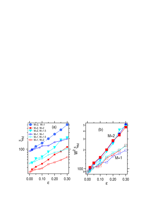
Figure 3: (Color online) (a)Localization length $\xi_{M}$ of the A-model as a function of perturbation strength $\epsilon$ for $M=1,2$ and $W=1.0,1.5,2.0$. (b) $\xi_{M}W^{2}$ as a function of $\epsilon$. Note that the vertical axes are logarithmic scale.

III.4 $\epsilon-$dependence of localization length for large $\epsilon$

We observed that, at least, the wavepacket localizes completely when $M=2$ in the region where the perturbation strength is relatively small $\epsilon<0.4$. We would like to investigate the localization length $\xi_{M}$ for $M=1$ and $M=2$ when $\epsilon$ increases beyond the perturbation region. In the region where $\epsilon$ is large, the localization length $\xi_{M}$ cannot be estimated directly by the saturation level of the MSD.
Here, we try to determine $\xi_{M}$ indirectly by supposing that the MSD data follows the common scaling from independent of $\epsilon$ as

$$m_{2}(t)\sim\xi(\epsilon)^{2}F\left(\frac{t}{\xi(\epsilon)^{2}}\right),$$ (13)

where $F(x)$ is a scaling function. To confirm this, we show in Fig.4 the plots of $m_{2}/\xi(\epsilon)^{2}$ as a function of $t/\xi(\epsilon)^{2}$, which manifests the scaling hypothesis of Eq.(13).

We can estimate the localization length $\xi_{M}(\epsilon)$ by using, and sometimes by repeatedly using, the scaling hypothesis Eq.(13) even for $\epsilon>0.4$.

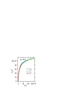
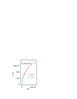
Figure 4: (Color online) Scaling peoperty $m_{2}(t)/\xi(\epsilon)^{2}$ as a function of $t/\xi(\epsilon)^{2}$ in the dichromatically perturbed A-model of $W=1$ for various $\epsilon$’s. (a)$\epsilon=0.40,0.50,0.55,0.60$ and (b)$\epsilon=0.55,0.70,0.80$.

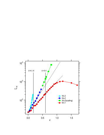
Figure 5: (Color online) Localization length as a function of $\epsilon$ for $M=1,2,3$ with $W=1$. Some LL of $M=2$ are obtained by the scaling hypothesis Eq.(13) for $\epsilon>0.4$. Note that the horizontal axis is in logarithmic scale. The dashed lines are $e^{5.5\epsilon}$ and $e^{3.8\epsilon}$, respectively. The lines $\epsilon=0.18$ and $\epsilon=0.6$ are shown as a reference.

Figure 5 shows the $\epsilon-$dependence of a wide range of the localization lengths, including indirectly determined $\xi_{M}$ with the scaling hypothesis (13). For comparison, $\xi_{M}$ of $M=3$, which exhibits a clear DLT as discussed in detail later, is also shown.The localization, of course, occurs in the case of $M=1$.

Then what is the difference of the localizations between the case of $M=1$ and the cases of $M=2$. In both cases of $M=1$ and $M=2$, the localization length grow exponentially when the $\epsilon$ is small enough ($\epsilon<0.8$ for $M=1$ and $\epsilon<0.3$ for $M=2$).

For $M=1$, it is obvious that the localization occurs no matter how large $\epsilon$ may be, but, as for $M=2$, the presence or absence of DLT is still unclear. We will discuss again the persistence of localization for $M=2$ in Sect. V after the next Sect.IV in which the presence of DLT is confirmed for $M\geq 3$. In the next subsection we consider the substantial dimension of our system which may dominate the upperbound dimension of localization.

III.5 The effective dimension

Our model (1) is very similar to that of the AM perturbed by $M$ harmonic modes, which is represented by the symplectic propagator (5) of $\Delta t=1$ It is formally transformed into $d(=M+1)-$dimensional quasi-random lattice by the so called Maryland transformation yamada20 , and $d=2$, i.e. $M=1$, is the upper-bound of dimension in which deloclization does not happen. Unlike this, in the present model the numerical observations suggest $M=2$ may be the upper-bound dimension of the localization. Why is there such a difference is?

In the case of AM, time is not continuous and there is no conserved quantity. However, in the present case, Eq.(1) is rewritten as Eq.(B) given in Appendix B which yields a severe constraint of energy conservation. In the transition process by the interaction among the harmonic modes and the isolated 1D random lattice the constraint due to the energy conservation

$$\left|\sum_{m=1}^{M}\Delta n_{m}\omega_{m}\right|<\frac{|E_{N}-E_{N^{\prime}}|}{\hbar}<\frac{C}{\hbar}$$ (14)

exists, where $E_{N}$ and $E_{N^{\prime}}$ are the energies of the localized eigenstates and $\Delta n_{i}=n_{i}^{\prime}-n_{i}$ is the change of excitation number of $i$-th harmonic mode. The upper-bound of $C={\rm Max}\{|E_{N}-E_{N^{\prime}}|\}$ is estimated as $C<4+2W$. IF $C=0$, the number of degrees of freedom exactly reduces by exactly 1, and

$$d_{f}=(M-1)+1=M$$ (15)

is the effective dimension of the system. However, since $C$ is finite, the system should be regarded as the “quasi-$d_{f}$” dimensional system in the sense that $M-1$ quantum numbers can arbitrarily be changed but the $M$-th mode is restricted by Eq.(14). If $d_{f}$ corresponds to the spatial dimension of the irregular lattice, then the maximal dimension in which only the localization exist can be $d_{f}=M=2$ if the scaling theory of the localization is followed. In the present paper we interpret the results presented below on the hypothesis that Eq.(15) is the “effective dimension”. We emphasize that the hypothesis was not taken into account in our previous letter, and $M+1$, instead of $M=d_{f}$, was used as the system dimension yamada21 .

IV Localization-Delocalization transition: A-model

In this section, we investigate LDT of the A-model with increasing the number of colors from $M=3$ to $M=7$ while paying attention to the correspondence with result in the Anderson map system. The case of $M=2$, which has a large localization length but is expected to have no LDT, will be also rediscussed in next section.

IV.1 dynamical LDT

In Fig.6, typical examples indicating the LDT for $M\geq 3$ are depicted. They are the double logarithmic plot of the time evolution of MSD for an increasing series of the perturbation strength $\epsilon$. For both examples one can recognize that with an increase in $\epsilon$ the time evolution of MSD exhibits a transition from a saturating behavior to a straight line of slope 1 implying the normal diffusion $m_{2}\propto t$. A remarkable fact is that the transition proceeds through a time evolution represented by a straight increase with a fractional slope $0<\alpha<1$ at a particular value $\epsilon=\epsilon_{c}$. It can be regarded as the critical subdiffusion $m_{2}\propto t^{\alpha}$. Indeed, for $M\geq 3$ the numerical results indicate that the asymptotic behavior of the MSD in the limit $t\to\infty$ changes as

$$m_{2}(t)\sim\begin{cases}t^{0}{\rm(localization)}&\epsilon<\epsilon_{c}\\ t^{\alpha}{\rm(subdiffusion)}&\epsilon\simeq\epsilon_{c}\\ t^{1}{\rm(delocalization)}&\epsilon>\epsilon_{c}\end{cases}$$ (16)

which fully follows the numerical observations in AM and SM yamada20 .

To confirm numerically the critical behavior represented by Eq.(16), it is very convenient to introduce the local diffusion exponent defined as the instantaneous slope of the log-log plot of MSD

$$\alpha_{ins}(t)=\dfrac{d\log m_{2}(t)}{d\log t}.$$ (17)

as a function of $t$, where $m_{2}(t)$ is appropriately smoothed.

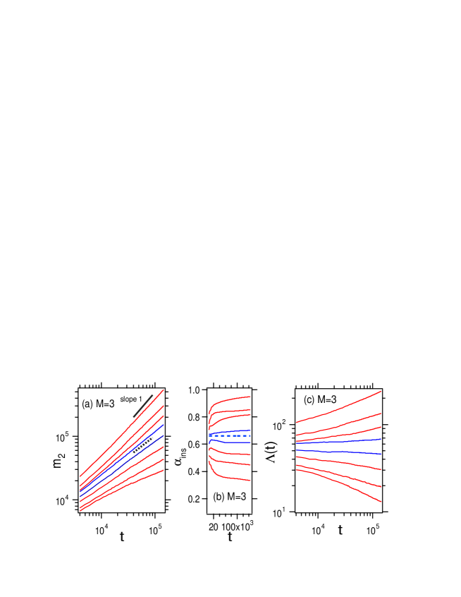
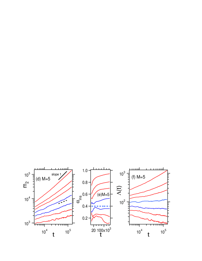
Figure 6: (Color online) Localization-delocalization transition for the A-model exhibited by the change of time-dependence of MSD: (a),(b), and (c) for $M=3$ and $W=1$ and (d),(e) and (f) for $M=5$ and the same $W=1$. (a) The double-logarithmic plots of MSD $m_{2}(t)$, (b) the diffusion index $\alpha_{ins}(t)$ and (c) the scaled MSD $\Lambda(\epsilon,t)=m_{2}(t)/t^{\alpha_{c}}$, where $\alpha_{c}=0.66$ as functions of time for increasing perturbation strengths $\epsilon=0.17,0.18,0.19,0.20,0.21,0.22,0.23,0.25$ from below. The broken line in (b) indicates the critical subdiffusion line $\alpha_{ins}(t)=\alpha_{c}=0.66$ predicted by the scaling theory. (d)(e) and (f) are the counterparts of (a)(b) and (c), respectively, for $M=5$, where $\epsilon$ is increased as $\epsilon=0.05,0.06,0.07,0.08,0.09,0.10,0.12$ from below and $\alpha_{c}=0.40$.

Figure 6(a)-(c) and (d)-(f) are examples of the transition process modeled by Eq.(16) for $M=3$ and $M=5$, respectively. (a) and (d) represent the change of MSD from the localized states to the normal diffusion state. Transition from the localized state to the normal diffusion is directly recognized by the change of $\alpha_{ins}(t)$ plots demonstrated in (b) and (e). It either decays to 0 or increases toward 1, and it keeps a constant value only at a particular $\epsilon=\epsilon_{c}$, indicated by broken lines, which means the existence of the critical subdiffusion $m_{2}(t)\propto t^{\alpha_{c}}$ at $\epsilon=\epsilon_{c}$, where $0.60<\alpha_{c}<0.70$ and $0.35<\alpha_{c}<0.45$ in (b) and (e), respectively.

These facts suggest the so called one-parameter scaling theory, which was successfully used in the analyses of AM and SM, is applicable to our model, identifying the effective dimension Eq.(15) as the dimension $d$ of the random system. It predicts the critical subdiffusion index as

$$\alpha=\frac{2}{d_{f}}=\frac{2}{M}.$$ (18)

The theoretical value $\alpha\sim 0.66$ for $M=3$ and $\alpha\sim 0.40$ for $M=5$ are drawn in (b) and (e) by broken lines, respectively. Agreement with the critical lines suggested by $\alpha_{ins}(t)$ plots is evident. We note that in our preliminary report we took $d_{f}=M+1$, instead of Eq.(15), because the restriction (14) was not taken into account. However, as $M$ increases beyond 5, Eq.(18) become less cofirmative.

To make a further check of the LDT close to the critical point, it is instructive to use the MSD $\Lambda(t)$ divided by the critical subdiffusive increase:

$$\Lambda(t)\equiv\dfrac{m_{2}(t)}{t^{\frac{2}{M}}}.$$ (19)

Then $\Lambda(t)\simeq const.$ indicates the critical point, and $\Lambda(t)$ grows upward for $\epsilon>\epsilon_{c}$, while it decays downward for $\epsilon<\epsilon_{c}$, as are seen in Fig.6(c) and (f). The feature that the $\Lambda(t)$ curves expands to form a trampet-like pattern suggests the existence of the LDT.

As are shown in Fig.7, we confirm that the critical sub- diffusion can be observed at certain critical point $\epsilon=\epsilon_{c}$ even if $M$ is increased beyond 3, and it is evident that the subdiffusion index $\alpha$ at the critical point decreases as $M$ increases, and it is numerically consistent with the prediction of Eq.(18).

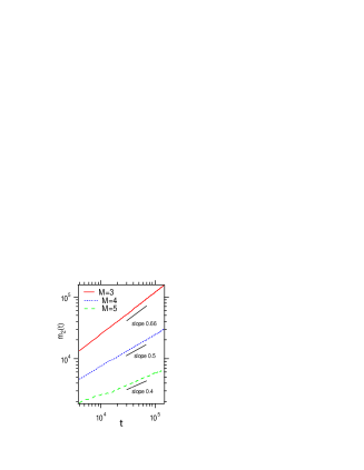
Figure 7: (Color online) The double-logarithmic plots of $m_{2}(t)$ as a function of time near the critical pints $\epsilon_{c}$ in the polychromatically perturbed 1D Anderson model ($M=3,4,5$ from top) with $W=1$.

IV.2 $M-$dependence of the scaling property for the LDT

In Fig.8(a), we show result of finit-time scaling analysys for the A-model of $M=3$. The method used here is the same as that used in the paper yamada20 . We choose the following quantity as a scaling variable

$$\Lambda_{s}(\epsilon,t)=\log\Lambda(\epsilon,t)=F(x),$$ (20)

by shifting the time axis to $x$:

$$x=\xi_{M}(\epsilon)t^{\alpha/2\nu},$$ (21)

for different values of $\epsilon$ by using critical exponent $\nu$ to characterize the divergence of the localization length around the LDT:

$$\xi_{M}\sim|\epsilon-\epsilon_{c}|^{-\nu}.$$ (22)

$F(x)$ is a differentiable scaling function and $\alpha$ is the diffusion index.

Figure 8(b) shows a plot of $\Lambda_{s}(t)$ as a function of $\epsilon$ at several times $t$, and it can be seen that this intersects at the critical point $\epsilon_{c}$. In addition, Fig.8(c) shows a plot of

$$s(t)=\frac{\Lambda_{s}(\epsilon,t)-\Lambda_{s}(\epsilon_{c},t)}{|\epsilon_{c}-\epsilon|}\propto t^{\alpha/2\nu}$$ (23)

as a function of $t$, and the critical localization exponent $\nu$ is determined by best fitting this slope. This is consistent with formation of the one-parameter scaling theory (OPST) of the localization. As a result, even in the A-model, the OPST is well established for the LDT regardless of the number of colors $M$ and the disorder strength $W$.

The critical exponent evaluated using the data ($\alpha=0.66,\epsilon_{c}=0.21$) at $W=1$ for $M=3$ is $\nu\simeq 1.81$. The same is true for the other $M(\geq 4)$ color perturbations. Appendix D shows the results of the finite-time scaling analysis when $M=4$ and $M=7$. These results are similar to that of AM system perturbed by the $(M-1)$ colors and of numerical calculations using finite-size scaling in the $d_{f}(=M)-$dimensional random systems. Note that pursuing the numerical value of $\nu$ with high accuracy is not the purpose of this paper.

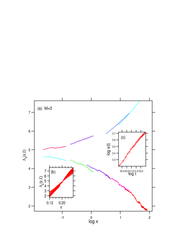
Figure 8: (Color online) The results of the critical scaling analysis for trichromatically perturbed A-model ($M=3$) with $W=1.0$. (a)The scaled MSD $\Lambda_{s}(\epsilon,t)=\log\Lambda(\epsilon,t)$ as a function of $x=\xi_{M}(\epsilon)t^{\alpha/2\nu}$ for some values of $\epsilon$. (b)The scaled $\Lambda_{s}(\epsilon,t)$ with $\alpha=0.66$ as a function of $\epsilon$ for some pick up times. The crossing point is $\epsilon_{c}\simeq 0.21$. (c)$s(t)$ as a function of $t$. The critical exponent $\nu\simeq 1.81$ is determined by a scaling relation Eq.(23) by the least-square fit.

IV.3 $M-$dependence of critical strength $\epsilon_{c}$

Return to the story of critical perturbation strength $\epsilon_{c}$. As is seen in Fig.9(a), $\epsilon_{c}$ definitely decreases with increase in $M$ for $M\geq 3$. Looking upon $\epsilon_{c}$ as the function of $M-2$, the double-logarithmic plots are on a straight line with the approximate tangent $-0.5$, namely

$$\epsilon_{c}\sim\frac{1}{(M-2)^{\delta}},~{}~{}\delta\simeq 0.5,$$ (24)

This result suggests that $\epsilon_{c}$ diverges at $M=2$, and the LDL transition do not exists at $M=2$. Evident dependence of $\epsilon_{c}$ on $M$ for large $M$ contradict with the prediction of the SCT yamada20 .

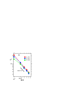
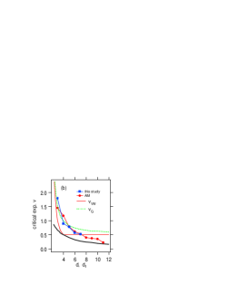
Figure 9: (Color online) (a)The critical perturbation strength $\epsilon_{c}$ as a function of $(M-2)$ for A-model with $W=1$. The black solid line shows $\epsilon_{c}\propto 1/(M-2)^{0.5}$. (b)The effective dimensionality $d_{f}=M$ dependence of the critical exponent $\nu$ which characterizes the critical dynamics. The red solid line and green dashed line are the results of the analytical prediction by $\nu_{VW}$ and $\nu_{G}$, respectively. Thick line denotes the lower bound by the Harris’ critical inequality.

The critical exponent $\nu$, which characterizes the divergence of the localization length at the critical point is numerically evaluated, and plotted against $M$, as shown in Fig.9(b). As a result, it can be seen that the tendency for $M\geq 3$ is close to that in the Anderson map.

IV.4 $W-$dependence of the critical point $\epsilon_{c}$

Figure 10 shows the $W-$dependence of the critical perturbation strength $\epsilon_{c}$ for $M=4$,$M=5$ and $M=6$. From this result, it can be inferred that the critical perturbation strength $\epsilon_{c}$ of the LDT keeps an almost constant value insensitive to the disorder strength $W$ and is only determined by the number of colors $M$. Such a feature agrees with that observed in the Anderson map system with $M\geq 2$ for which the LDT emerges.

Figure 10: (Color online) The critical perturbation strength $\epsilon_{c}$ as a function of $W$ in A-model of $M=4,5,6$ (from top).

We show another direct evidences manifesting that the magnitude of $W$ does not influence the LDT. The time evolution of the MSD at $\epsilon_{c}$ is shown for several values of $W$ in Fig.11. First, looking at the case of $M=4$ in Fig. 11(a) the spread $m_{2}(t)$ of wavepacket becomes larger with decrease in $W$, as is expected. But in all case we see that for the same $\epsilon=\epsilon_{c}=0.115$ a subdiffisive increase at the same index $\alpha\simeq 0.5$ emerge regardless of $W$. Similarly, in the case of $M=6$, regardless of $W$, for the same $\epsilon_{c}\simeq 0.058$ the subdiffusion of $\alpha\simeq 0.33$ emerges, as are seen in Fig.11(c).

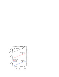
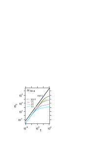
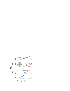
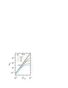
Figure 11: (Color online) The double-logarithmic plots of $m_{2}(t)$ as a function of time $t$ near the critical pints $\epsilon_{c}$ for different $W$ in the A-model of (a)$M=4$ and of (c)$M=6$. The panels (b) and (d) show the enlarged view of the short-time region $t<10^{2}$ in the double-logarithmic plots of $m_{2}(t)$ in the A-model of (b)$M=4$ and (d)$M=6$.

Figure 11(b) and (d) are the enlargement of the initial growth of MSD for $t<10^{2}$ of (a) and (c), respectively. In all cases, the wavepacket starts with a ballistic expansion $m_{2}\sim t^{2}$ and changes to exhibit the critical subdiffusion after a lapse of characteristic time. A paradoxical fact is that the characteristic time required for realizing the subdiffusive delocalization decreases with increase in the disorder strength $W$.

The larger the $W$, the stronger the localization, and as the localization becomes stronger, delocalization occurs more promptly. This means that what is important for delocalization is not to activate the ballistic expansion of the wavepacket, but to promote its decomposition into particle-like quantum states called localized states due to the accumulation of scattering by disorder. Delocalization emerges as the diffusive motion over the localized particle-like states.

V Reconsideration of weak dynamical localization for $M=2$

We return to the problem on the presence of DLT in the case of $M=2$.

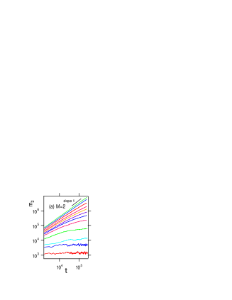
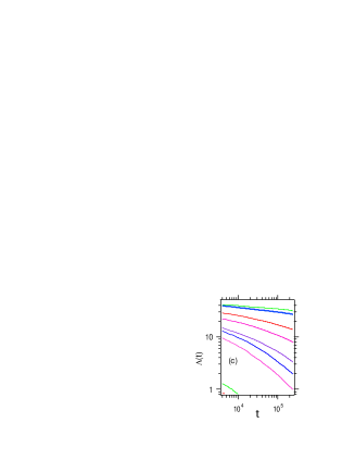
Figure 12: (Color online) (a)The double-logarithmic plots of $m_{2}(t)$ as a function of time for some values of the perturbation strength $\epsilon$ increasing from $\epsilon=0.1$ to $\epsilon=1.3$ in the A-model of $M=2$ with $W=1$. (b)The instantaneous diffusion index $\alpha_{ins}(t)$ as a function of time. (c)The double-logarithmic plots of the scaled MSD $\Lambda(\alpha=1,t)=\frac{m_{2}(t)}{t}$ as a function of time for some $\epsilon^{\prime}s$ from $\epsilon=0.1$ to $\epsilon=1.3$.

It is very hard to numerically prove the persistence of localization, either by directly pursuing time evolution dynamics or by applying the scaling hypothesis. (See Fig.12(a).) However, there are some evidences manifesting that there exists no critical subdiffusion such that $m_{2}\propto t^{\alpha}$ with $0<\alpha<1$. To numerically prove the presence of critical subdiffusion, an explicit method is to use the $\alpha_{ins}(t)$ plots presented in the previous section. We examine in Fig.12(b) the $\alpha_{ins}(t)$ plots for $M=2$. All the curves go downward and it can hardly be expected that a horizontal line locates in the narrow gap between the line $\alpha=1$ and the uppermost downward curve, which implies that $\alpha=1$ plays the role of “critical diffusion”. This fact is consistent with the results of previous section represented by Eq.(18) and Eq.(24) for $M\geq 3$, which predict $\alpha=1$ and $\epsilon_{c}=\infty$, respectively, for $M=2$.
We further examine in Fig.12(c), the $\Lambda$ plots Eq.(19), namely the MSD scaled by the critical MSD $m_{2}(t)\propto t^{\alpha}$, which is $\Lambda(\alpha=1,t)=\frac{m_{2}(t)}{t}$ supposing $\alpha=1$. All the curves go downward for $t>>1$ to form the lower-half of the pre-critical trampet pattern shown in Figs.6(c) and (f) for $M\geq 3$. All the above results allows us to regarded the normal diffusion $m_{2}(t)\propto t$ as an ultimate limit of the critical subdiffusion for $M=2$, and $d_{f}=M=2$ is just the critical dimension of localization exhibited by the A-model.

Furthermore, we confirmed that the above features do not change when the radom potential $V(n,t)$ is replaced by

$$V(n,t)=V_{1}(n)+V_{2}(n)f_{\epsilon}(t),$$ (25)

where $V_{1}(n)$ and $V_{2}(n)$ are different random sequences. The same is true if a binary random sequences taking $-W$ or $W$. are used for $V_{1}(n)$ and $V_{2}(n)$.

VI Delocalized states

In this section, we investigate the characteristics of the delocalized states which emerges for $M\geq 3$ and $\epsilon>\epsilon_{c}$ in comparison with the stochastic model. Results are compared also with the B-model with no static random potential.

VI.1 Comparison with stochastic models

We investigate the dependency upon the two parameters $W$ and $\epsilon$ in comparison with the $D$ of the stochastic model by Haken and others haken72 ; palenberg00 ; moix13 ; knap17 .

Typical examples of the $m_{2}(t)$ for $\epsilon>>\epsilon_{c}$ in the cases of $M=3$ and $M=7$ are shown in Fig.14(a) and (b), respectively. If $\epsilon$ is large enough, it is evident that MSD follows asymptotically the normal diffusion $m_{2}=Dt$, which implies that only finite number of coherent modes plays the same role as the stochastic perturbation.

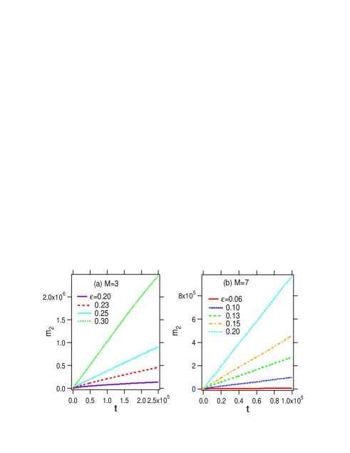
Figure 13: (Color online) The $m_{2}(t)$ as a function of time in the A-model of (a)$M=3$ and (b)$M=7$ with $W=1$ for some values of the perturbation strength $\epsilon$, increasing from $\epsilon=0.1$(bottom) to $\epsilon=0.2$(top) for $M=7$ and from $\epsilon=0.2$(bottom) to $\epsilon=0.3$(top) for $M=3$, respectively. Note that the axes are in the real scale.

Indeed, the $W-$dependence of the diffusion coefficient $D$ depicted in Fig.14 follows the main feature of the stochastically induced diffusion constants regardless of the number of colors $M(\geq 3)$. The dependence changes in the weak regime and strong regime of $W$ as

$$D\propto\begin{cases}W^{-2}&(W\ll 1)\\ W^{-4}&(W\gg 1).\end{cases}$$ (26)

The weak regime result follows Eq.(8) if $W\gg\epsilon$. The strong regime behavior agrees with the result obtained by Moix et al moix13 for the stochastic model in the very large limit of $W$.

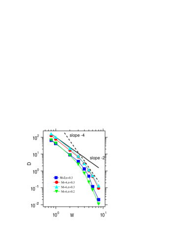
Figure 14: (Color online) The diffusion coefficient $D$ of the quantum diffusion as a function of $W$ in the A-model with $\epsilon=0.2$ or $\epsilon=0.3$ of $M=3,4,6$. Note that the axes are in the logarithmic scale. $D\propto W^{-2}$ and $D\propto W^{-4}$ are shown by black line and black dotted lines, respectively, for reference.

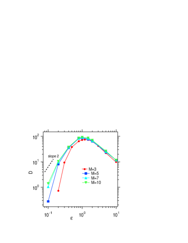
Figure 15: (Color online) The diffusion coefficient $D$ as a function of $\epsilon$ for the A-model with $W=1$ and $M=3,5,7,10$. Note that the axes are in the logarithmic scale. $D\propto\epsilon^{2}$ is shown by black line for reference.

Next, we examine the $\epsilon$-dependence of $D$, which is shown in Fig.15 for some $M$s. As a whole, the $\epsilon$-dependence almost follows Eq.(8) for all $M$. (We note that Eq.(8) is valid for small $\epsilon$ and $W$, and it can not be directly be applied to the interpretation of our result.) If $\epsilon$ is weak $D$ increases as

$$D\propto\epsilon^{2}$$ (27)

for $M\gg 1$ in agreement with Eq.(8), and after going over the maximum value at $\epsilon^{*}\sim O(1)$, it decreases. In particular in the regime $\epsilon>\epsilon^{*}$, $D$ has no significant $M$-dependence. This fact implies a remarkable feature that the diffusion induced by the coherent perturbation composed of only three incommensurate frequencies mimics the normal diffusion induced by a stochastic perturbation containing infinite number of colors.

VI.2 Comparison with the B-model

In the case of $\epsilon=0$, the B-model becomes spatially periodic system without potential part, and the wavepacket exactly shows ballistic motion as $m_{2}(t)\propto t^{2}$. We consider the MSD for finite $\epsilon$ in the B-model in comparison with the A-model. Figure.16(a) shows the time evotution of the MSD of the B-model with $M=3$ for some values of $\epsilon$. We can see the ballistic growth $m_{2}(t)\sim t^{2}$ in the short time regime in the all cases. As seen in the $M-$dependence in the Fig.16(b), in the B-model of $M=1$, the wavepacket localizes. In contrast, for $M\geq 2$ the normal diffusive behavior $m_{2}\propto t$, which loses significant $M$-dependence, appears as time proceeds. For more detailed features of MSD of the B model, see Appendix E.

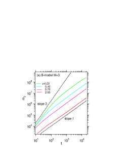
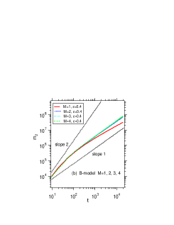
Figure 16: (Color online) The double-logarithmic plots of $m_{2}(t)$ as a function of $t$ in the B-model with $W=1$. (a)$M=3,W=1$. (b)$M=1,2,3$ and $W=1$. Note that the axes are in the logarithmic scale. Black dotted line shows $m_{2}(t)\propto t^{1}$ for reference.

Figure 17 compares the $\epsilon-$dependence of the diffusion coefficients $D$ of the B-model with those of the A-model. The difference between A-model and B-model is evident in the region $\epsilon_{c}<\epsilon<\epsilon^{*}$. In A-model, as was stated above, $D$ increases first like $\epsilon^{2}$ in $\epsilon<\epsilon^{*}$ and it decreases beyond $\epsilon^{*}$. But in B-model $D$ decreases monotonously. In the regime $\epsilon<\epsilon^{*}$, $D$ decreases in contrast to Eq.(27) as

$$D\propto\epsilon^{-2}$$ (28)

Beyond $\epsilon^{*}$, $D$ continues to decreases, which is closely followed by A-model. Thus the diffusion processes of the two models become indistinguishable in the region $\epsilon\gg\epsilon^{*}$ for $M\geq 3$. The above tendency is the same even when we examine the the stochastic model by replacing $f_{\epsilon}(t)$ with $n(t)$. For $\epsilon>\epsilon^{*}$, the $\epsilon-$dependence of the diffusion coefficient $D$ of the SA-model also approach those of the SB-model. (See Fig.22 in Appendix E.)

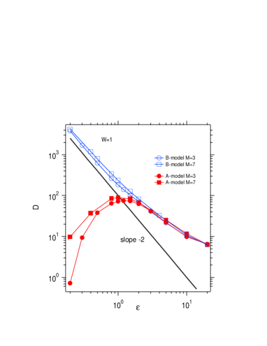
Figure 17: (Color online) The diffusion coefficient $D$ of the quantum diffusion as a function of $\epsilon$ in the A-model and B-model for several $M$ with $W=1$. The corresponding results for the ballistic model are also provided. Note that the axes are in the logarithmic scale. $D\propto\epsilon^{-2}$ is shown by black line for reference.

VII Summary and discussion

We investigated systematically the localization-delocalization transition (LDT) of the one-dimensional Anderson model which is dynamically perturbed by polychromatically quasi-periodic oscillations by changing the three parameters; the disorder strength $W$, perturbation strength $\epsilon$ and the number of the colors $M$ of the oscillations. The dynamical localization length (LL) was evaluated by the MSD computed by the numerical wavepacket propagation. Although our model consists of $M+1$ degrees of freedom, we analyzed the numerical results under the hypothesis that the effective dimension $d_{f}$ is $M$, not $M+1$, considering the energy conservation. The transition to delocalization is observed for $M=d_{f}+1\geq 3$, and for $M=d_{f}+1\leq 2$ only localization takes place, which are consistent with the $d-$dimensional Anderson model if $d_{f}$ is identified with $d$.

For $M\leq 2$ the LL increases exponentially with respect to $\epsilon$ if $\epsilon$ is relatively small. On the other hand, the $W-$dependence of the LL is also scaled by the disorder strength $W$ as in the case of Anderson map (AM).

For $M\geq 3$ the localization-delocalization transition(LDT) always takes place with increase in the perturbation strength $\epsilon$, and at the critical point $\epsilon_{c}$ the fractional diffusion MSD$\propto t^{\alpha}$ ($0<\alpha<1$) is observed. The critical diffusion exponent decreases as $\alpha\simeq 2/M$ with $M$ in accordance with the prediction of one-parameter scaling theory (OPST) under the hypothesis $d_{f}=M$. The numerical results reveal that the critical perturbation strength decreases as $\epsilon_{c}\propto 1/(M-2)^{1/2}$ with an increase of $M$. These properties are different from those of the AM system reported in the previous papers yamada20 . On the other hand, the dimensional dependence of the critical exponent $\nu$ of the localization length (LL) roughly estimated by the numerical data was qualitatively consistent result with those of the polychromatically perturbed AM system with $(M-1)$ colors and the LDT in $d-$dimensional Anderson model.

The Table 1 summarizes the localization and delocalization phenomena of the random systems, including the case of the random system of the spatial dimension $d$ and the perturbed quantum map systems.

We also studied the delocalized states for $\epsilon>\epsilon_{c}$. Even though $M$ is not large, the $W-$ and $\epsilon-$dependence of the diffusion coefficient of the delocalized states mimics those predicted for the stochastically perturbed 1D Anderson model.

As $\epsilon>O(1)$ the characteristics of diffusion of our model approaches closely to those of the B-model which contains only the quasi-periodically oscillating random potential and has no static randomness.

Table 1: Dimensionality of the DLT. For $4\leq M<\infty$ the result is same as the case of $M=3$. The lower lines is result of the $d-$dimensional disordered systems by the scaling theory of the localization. Loc: exponential localization, LDT:localization-delocalization transition, Diff:Normal diffusion.

$M$	0	1	2	3	4
this study(A-model)	Loc	Loc	Loc	LDT	LDT
this study(B-model)	Bali	Loc	Diff	Diff	Diff
Anderson map yamada20	Loc	Loc	LDT	LDT	LDT
Standard map yamada20	Loc	Loc	LDT	LDT	LDT
d	1	2	3	4	5
Anderson model	Loc	Loc	LDT	LDT	LDT

Appendix A Frequency set used in the calculation

Table 2 shows the sets, $S_{1}$,$S_{2}$,$S_{3}$, of the frequency set $\{\omega_{i}\}$. $S_{1}$ is mainly used in the text, and as mentioned in the text, which is set to be $O(1)$ in the incommensurate as much as possible. The frequency set relatively affects the numerical result compared to the case of the Anderson map system, although the larger the $M$, the smaller the influence of how to select the frequency. Therefore, in addition to the fundamental frequency set $S_{1}$, we investigated the result in the A-model with the other frequency sets $S_{2}$, $S_{3}$ given in the Table 2. Randomly chosen values are used for $S_{3}$. $S_{2}$ was used for numerical calculation by 6th order symplectic integrator in our previous paper yamada99 .

Table 2: The frequencies $S_{1}$ we mainly used are followings: $\omega_{1}=(1+\sqrt{5})/2$, $\omega_{2}=2\pi/\lambda$, $\omega_{3}=2\pi/\lambda^{2}$, $\omega_{4}=\sqrt{3}-1$, $\omega_{5}=\sqrt{2}-1$, $\omega_{6}=\sqrt{13}/2-1$, $\omega_{7}=\sqrt{11}-3$, $\omega_{8}=\sqrt{10}/2-1$, $\omega_{9}=5\sqrt{17}-20$, $\omega_{10}=2\sqrt{19}/2-1$, where $\lambda$ denotes the real root of the cubic equation $x^{3}-x-1=0$. We have checked for another set of the frequencies. The whole tendency of the main result in the present paper is not depend on the choice for the long-time calculation with large system size. $S_{2}$ and, $S_{3}$ are used to get the data of $M=6$ and $M=7$ for check. $r_{k}$($k=1...,7$) take uniform random number within $[0,1]$.

$\omega_{M}$	$S_{1}$	$S_{2}$	$S_{3}$
$\omega_{1}$	$\sigma$	1+$\sqrt{1/7}$	1/2+$r_{1}$
$\omega_{2}$	$\nu_{1}$	1+$\sqrt{2/7}$	1/2+$r_{2}$
$\omega_{3}$	$\nu_{2}$	1+$\sqrt{3/7}$	1/2+$r_{3}$
$\omega_{4}$	$\sqrt{3}-1$	1+$\sqrt{5/7}$	1/2+$r_{4}$
$\omega_{5}$	$\sqrt{2}-1$	1+$\sqrt{7/7}$	1/2+$r_{5}$
$\omega_{6}$	$\sqrt{13}/2-1$	1+$\sqrt{10/7}$	1/2+$r_{6}$
$\omega_{7}$	$\sqrt{11}-3$	1+$\sqrt{11/7}$	1/2+$r_{7}$
$\omega_{8}$	$\sqrt{10}/2-1$	—	—
$\omega_{9}$	$5\sqrt{17}-20$	—	—
$\omega_{10}$	$2\sqrt{19}/2-1$	—	—

Appendix B Autonomous representation of the time-dependent Schrödinger equation (1)

Let the wavefunction describing the whole system composed of the one-dimensional lattice and the $M$ harmonic modes be $|\Psi(t)\rangle$. We introduce the set of the action-angle operators $(\hat{J}_{i},\hat{\phi}_{i}):=(-i\hbar\frac{\partial}{\partial\phi_{i}},\phi_{i})~{}~{}(i=1,2..M)$ representing the harmonic modes, and let $\hat{H}_{0}$ be the part of Hamiltonian in Eq.(1) without the harmonic perturbations (i.e. $\epsilon=0$) and introduce the Hamiltonian $\hat{h}=\sum_{i=1}^{M}\omega_{i}\hat{J}_{i}$ representing the harmonic modes. The autonomous version of Eq.(1) is written as the evolution equation:

$$i\hbar\frac{|\partial\Psi(t)\rangle}{\partial t}=\hat{H}_{\rm tot}|\Psi(t)\rangle$$ (29)

of the whole system with the total Hamiltonian

$$\hat{H}_{\rm tot}=\hat{H}_{0}+\hat{h}+\frac{W\epsilon}{\sqrt{M}}\sum_{N}v_{n}|n\rangle\langle n|\sum_{i=1}^{M}\cos(\phi_{i}),$$ (30)

where $H_{0}=\sum_{n}(|n+1\rangle\langle n|+|n\rangle\langle n+1|)+Wv_{n}|n\rangle\langle n|=\sum_{N}E_{N}|N\rangle\langle N|$ is the unperturbed Hamiltonian, and $|n\rangle$ is the base specifying the site $n$ of 1D Anderson model. The eigenstate of the action operator, which is angle-represented as $\langle\phi_{i}|J_{i}\rangle=e^{iJ_{i}\phi_{i}/\hbar}/\sqrt{2\pi}$ with the action eigenvalue $J_{i}=n_{i}\hbar$, is written as $|n_{i}\rangle$, and let the eigenstate of isolated one-dimensional lattice $H_{0}$ be $|N\rangle$ with eigenvalue $E_{N}$: $H_{0}|N\rangle=E_{N}|N\rangle$. By decomposing the quantum state of the total system as $|\Psi(t)\rangle=\sum_{N,\{n_{i}\}}\Psi(N,\{n_{i}\})|N,\{n_{i}\}\rangle$ Eq.(30) is rewritten by Eq.(1).

Let $\hat{U}_{\rm tot}={\rm exp}\{-i\hat{H}_{\rm tot}t/\hbar\}$ be the unitary evolution operator of the total system, and introduce the new operator $\hat{U}$ by $\hat{U}_{\rm tot}={\rm e}^{-i\hat{h}t/\hbar}\hat{U}$. Then the evolution equation

$$i\hbar\frac{\partial\hat{U}}{\partial t}=\left[H_{0}+\frac{W\epsilon}{\sqrt{M}}\sum_{n}v_{n}|n\rangle\langle n|\sum_{i=1}^{M}\cos(\omega_{i}t+\phi_{i})\right]\hat{U}$$

is immediately obtained, which is equivalent to Eq.(1) if the phase-eigenstate $|\phi_{1}\rangle,|\phi_{2}\rangle,....|\phi_{M}\rangle$ is supposed at $t=0$. The identity

$${\rm e}^{i\hat{J}\omega t/\hbar}{\rm e}^{-iK\cos\phi/\hbar}{\rm e}^{-i\hat{J}\omega t/\hbar}={\rm e}^{-iK\cos(\phi+\omega t)/\hbar}$$ (31)

is used.

Appendix C An alternative representaton of Eq.(II)

Eq.(30) allows us to introduce an alternative representation of Eq.(II) based upon the quantum state of a single lattice site dressed with harmonic modes interacting with it. We demonstrate the $M=1$ case. Let us focus on the part of Hamiltonian (30), from which the transfer term $\sum_{n}(|n+1\rangle\langle n|+|n\rangle\langle n+1|)$ is neglected,

$$\hat{H}^{(n)}=\omega\hat{J}+Wv_{n}(1+\epsilon\cos\phi)|n\rangle\langle n|,$$ (32)

which represents the $n$-site interacting with the harmonic mode. We set $\omega_{1}=\omega$. Suppose its eigenstates of the form $|n,K\rangle=|n\rangle|K\rangle_{n}$, satisfying $\hat{H}_{n}|n,K\rangle=E_{n,K}|n,K\rangle$, where $K$ is the new quantum number associates with the harmonic mode to be introduced later. One can readily find that the $\phi$-representation $\langle\phi|K\rangle_{n}:=u_{K,n}(\phi)$ of $|K\rangle_{n}$ satisfies the simple equation

$$i\omega\frac{\partial u_{K,n}}{\partial\phi}=\left[Wv_{n}(1+\epsilon\cos\phi)-E_{n,K}\right]u_{K,n},$$ (33)

which leads to

$$u_{K,n}(\phi)=\frac{1}{\sqrt{2\pi}}{\rm exp}\left[i\frac{(E_{n,K}-Wv_{n})\phi-Wv_{n}\epsilon\sin\phi}{\hbar\omega}\right],$$ (34)

where the quantization condition $E_{n,K}-Wv_{n}=K\omega\hbar$  ($K$ is an arbitrary integer) is required for the $2\pi$-periodicity of $u_{K,n}(\phi)$. Using the new basis $|n,K\rangle=|n\rangle|K\rangle_{n}$ we expand the wavefunction as $\Psi(t)=\sum_{n,K}\Phi(n,K)|n,K\rangle$, and the Schödinger equation in Eqs.(29) and (30) is rewritten into the following form, instead of the Eq.(II) with $M=1$,

$$i\hbar\frac{d\Phi(n,K)}{dt}=(K\omega\hbar+Wv_{n})\Phi(n,K)$$

$$+\sum_{K^{\prime}}\left[T_{K-K^{\prime}}^{n,n+1}\Phi(n+1,K^{\prime})+T_{K^{\prime}-K}^{n,n-1}\Phi(n-1.K^{\prime})\right].$$

Then the effective position dependent hopping is given as

$$T_{K-K^{\prime}}^{n,n^{\prime}}:=_{n}\langle K|K^{\prime}\rangle_{n^{\prime}}=J_{K-K^{\prime}}\left(\frac{\epsilon W(v_{n}-v_{n^{\prime}})}{\hbar\omega}\right),$$ (36)

where $J_{n}(x)$ is the first kind of Bessel function. We can see that the monochromatic perturbation combined the randomness is completely incorporated into the hopping terms. The amplitude $\Phi(n,K)$ at the each lattice site $(n,K)$ is connected to those at the sites $(n\pm 1,K-K^{\prime})$. It follows that for $\epsilon W/\hbar\omega<<1$ the hopping coefficients decay along the $K-$direction, and the system becomes quasi-1D tight-binding model because $J_{n}(x)\sim\frac{x^{n}}{2^{n}n!}$ as $n\to\infty$.

Similarly, in the case of the B-model of $M=1$, the model can be converted into a tight-binding model without the on-site randomness and with hopping randomness.

Appendix D Result of finite-time critical scaling analysis

Figure 18 and 19 displays the results of the finite-time scaling analysis for the A-model of $M=4$ and $M=7$, respectively. As a result, the OPST is well established for the LDT regardless of the number of colors $M$ and the disorder strength $W$.

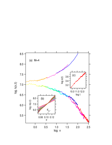
Figure 18: (Color online) The results of the critical scaling analysis for the A-model of $M=4$ with $W=1.0$. (a)The scaled MSD $\Lambda(\epsilon,t)$ as a function of $x=\xi_{M}t^{\alpha/2\nu}$ in the logarithmic scale for some values of $\epsilon$, where $\xi_{M}$ is the localization length as a scaling parameter . (b)The scaled $\Lambda(t)$ with $\alpha=0.5$ as a function of $\epsilon$ for some pick up times. The crossing point is $\epsilon_{c}\simeq 0.115$. (c)$s(t)$ as a function of $t$. The critical exponent $\nu\simeq 0.9$ is determined by a scaling relation Eq.(23) by the least-square fit.

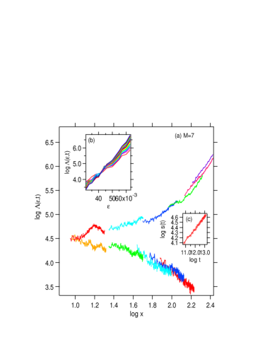
Figure 19: (Color online) The results of the critical scaling analysis for the A-model of $M=7$ with $W=1.0$. (a)The scaled MSD $\Lambda(\epsilon,t)$ as a function of $x=\xi_{M}(\epsilon)t^{\alpha/2\nu}$ in the logarithmic scale for some values of $\epsilon$, where $\xi_{M}$ is the localization length as a scaling parameter. (b)The scaled $\Lambda(t)$ with $\alpha=0.28$ as a function of $\epsilon$ for some pick up times. The crossing point is $\epsilon_{c}\simeq 0.042$. (c)$s(t)$ as a function of $t$. The critical exponent $\nu\simeq 0.52$ is determined by a scaling relation Eq.(23) by the least-square fit.

Appendix E Normal diffusion of the B-model

Unlike the A-model, in the B-model the system starts with the ballistic motion $m_{2}\propto t^{2}$, and the motion gradually changes as the perturbation becomes effective. The time-dependence of MSD of $M=1$ and $M=2$ is shown in Fig.20. As shown in the Fig.20(a), in the case of $M=1$, irrespective of the magnitude of $\epsilon$, the double-logarithmic plots of $m_{2}(t)$ tells that its instantaneous slope $\alpha_{inst}(t)$ finally decreases gradually below $\alpha=1$, and we can not find any sign that $\alpha_{inst}(t)$ converges to a non-zero value. We, therefore, conjecture that delocalization does not occur for $M=1$.

On the other hand, in the case of $M=2$, as shown in Fig.20(b), the time domain in which the ballistic motion is taking place is reduced by increasing $\epsilon$, and normal diffusion, $m_{2}(t)\simeq Dt$, finally appears. (Due to the system size of numerical calculation, it tends to be saturated when it reaches the boundary.) We conjecture that, no matter how small the magnitude of $\epsilon$ may be, the ballistic motion $m_{2}(t)\simeq t^{2}$ changes into diffusive motion $m_{2}(t)\simeq t^{1}$ in a long time limit, if the system size is infinite. Similar behavior can be expected also for $M\geq 3$, and there is no LDT.

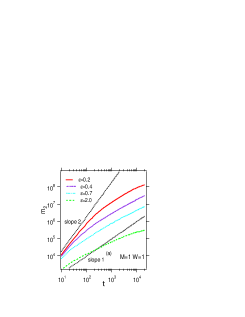
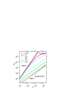
Figure 20: (Color online) The double-logarithmic plots of $m_{2}(t)$ as a function of $t$ for different values of $\epsilon$ in the B-model with $W=1$. (a)$M=1$ and (b)$M=2$. Black dotted and thick lines show $m_{2}(t)\propto t^{2}$ and $m_{2}(t)\propto t^{1}$, respectively, for reference.

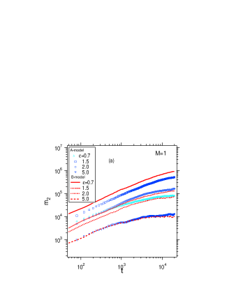
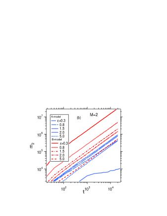
Figure 21: (Color online) The double-logarithmic plots of $m_{2}(t)$ as a function of $t$ for different values of $\epsilon$ in the A-model and B-model with $W=1$. (a)$M=1$. (b)$M=2$.

Figure 21 shows a comparison of $m_{2}(t)$ for some $\epsilon$’s in the A-model and B-model. Figure 21(a) is for $M=1$. The MSD of the A-model increases as $\epsilon$ increases, but it turns to decreases for $\epsilon>\epsilon^{*}$, where $\epsilon^{*}\sim 1$ is the characteristic value given in the text. At $\epsilon>>\epsilon^{*}$, it can be seen that the $m_{2}(t)$ of the A-model approaches the result of the B-model, and it overlaps for $\epsilon=5$ with that of the B-model. Both cases becomes localized. As mentioned in the main text, it can be said that it is an asymptotic transition from the A-model to the B-model as $\epsilon$ increases. Figure 21(b) is the result for $M=2$. In the $\epsilon=5.0$ both cases show normal diffusive behavior for $\epsilon>>1$.

Moreover, as can be seen in the localized case of the $\epsilon=0.7$ and $\epsilon=2.0$ in the A-model of $M=1$ in Fig.21 (a), the time dependence of $m_{2}(t)$ intersects. It follows that the two types of regions, $\epsilon<\epsilon^{*}$ and $\epsilon>\epsilon^{*}$, do not follow the same scaling curve towards localization even if the localization length is the same

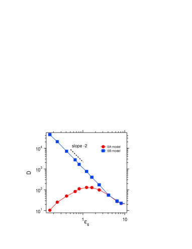
Figure 22: (Color online) The diffusion coefficient $D$ of the quantum diffusion as a function of $\epsilon$ in the SA-model and SB-model with $W=2.0$. Note that the axes are in the logarithmic scale and $\epsilon_{s}^{*}\simeq 1.15$ for $W=2$. $D\propto\epsilon_{s}^{-2}$ is shown by black dotted lines as a reference.

Figure 22 shows a comparison of the $\epsilon_{s}-$dependence of the diffusion coefficient in the SA-model and SB-model. It can be seen that the SA-model has a peak around $\epsilon_{s}^{*}\simeq 1.15$ and $D(\epsilon_{s})$ gradually approaches that of the SB-model for $\epsilon_{s}>>\epsilon_{s}^{*}$. This tendency is the same as the relationship between the A-model and the B-model.

References

- (1) P. W. Anderson, Phys. Rev. 109, 1492-1505 (1958).
- (2) K.Ishii, Prog. Theor. Phys. Suppl. 53, 77(1973).
- (3) L.M.Lifshiz, S.A.Gredeskul and L.A.Pastur, Introduction to the theory of Disordered Systems, (Wiley, New York,1988).
- (4) E. Abrahams (Editor), 50 Years of Anderson Localization, (World Scientific 2010).
- (5) P. Markos, Acta Phys. Slovaca 56, 561(2006).
- (6) Antonio M. Garcia-Garcia and Emilio Cuevas, Phys. Rev. B 75,174203(2007).
- (7) Yoshiki Ueoka, and Keith Slevin, J. Phys. Soc. Jpn. 83, 084711(2014).
- (8) E. Tarquini, G. Biroli, and M. Tarzia, Phys. Rev. B 95, 094204(2017).
- (9) D. Vollhardt and P. Wolfle, Phys. Rev. Lett. 45,842(1980). D. Vollhardt and P. Wolfle, Phys. Rev. B 22,4666(1980). D. Vollhardt and P. Wolfle, Phys. Rev. Lett. 48, 699(1982).
- (10) P. Wolfle and D. Vollhardt, Int. J. Mod. Phys B 24, 1526(2010).
- (11) H. Haken and P. Reineker, Z. Phys. 249, 253(1972). H. Haken and G. Strobl, Z. Phys. 262, 135(1973).
- (12) M. A. Palenberg, R. J. Silbey, and W. Pfluegl, Phys. Rev. B 62, 3744(2000).
- (13) J. M. Moix, M. Khasin and J. Cao, New Journal of Phisics 15, 085010(2013).
- (14) S. Gopalakrishnan, K. R. Islam, and M. Knap, Phys. Rev. Lett. 119, 046601(2017).
- (15) M. C. Gutzwiller, Chaos in Classical and Quantum Mechanics (Springer-Verlag, Berlin, 1991).
- (16) G.Casati, I.Guarneri and D.L.Shepelyansky, Phys. Rev. Lett. 62, 345(1989).
- (17) F.Borgonovi and D.L.Shepelyansky, Physica D109, 24 (1997).
- (18) C. Neill, et.al., Ergodic dynamics and thermalization in an isolated quantum system, Nature Physics 12, 1037-1041(2016).
- (19) Simone Notarnicola, Fernando Iemini, Davide Rossini, Rosario Fazio, Alessandro Silva, and Angelo Russomanno, Phys. Rev. E 97, 022202 (2018).
- (20) Angelo Piga, Maciej Lewenstein, James Q. Quach, Phys. Rev. E 99, 032213 (2019).
- (21) Kensuke Ikeda, Annals of Physics 227 1 (1993)
- (22) M.Lopez, J.F.Clement, P.Szriftgiser, J.C.Garreau, and D.Delande, Phys. Rev. Lett. 108, 095701(2012).
- (23) M. Lopez, J.-F. Clement, G. Lemarie, D. Delande, P. Szriftgiser, and J. C. Garreau, New J. Phys. 15, 065013(2013).
- (24) H.S.Yamada, F.Matsui and K.S. Ikeda, Phys.Rev.E 92, 062908(2015).
- (25) H.S.Yamada, F. Matsui and K.S.Ikeda, Phys.Rev.E 97, 012210(2018).
- (26) H.S.Yamada and K.S.Ikeda, Phys.Rev.E 101, 032210 (2020).
- (27) H.Yamada and K.S.Ikeda, Phys.Lett.A 248,179(1998).
- (28) H.Yamada and K.S. Ikeda, Phys.Rev.E 59,5214(1999).
- (29) M. Holthaus, G.H.Ristow, and D.W.Hone, Phys. Rev. Lett. 75, 3914(1995).
- (30) Dario F. Martinez and Rafael A. Molina, Phys. Rev. B 73, 073104 (2006).
- (31) H. Hatami, C. Danieli, J. D. Bodyfelt, S. Flach, Phys. Rev. E 93, 062205 (2016).
- (32) J. Bourgain,and W. Wang, Commun. Math. Phys. 248, 429 (2004).
- (33) H.S.Yamada and K.S.Ikeda, Phys.Rev.E 103, L040202(2021).