An Equivalence Between Data Poisoning and Byzantine Gradient Attacks

Abstract

To study the resilience of distributed learning, the “Byzantine” literature considers a strong threat model where workers can report arbitrary gradients to the parameter server. Whereas this model helped obtain several fundamental results, it has sometimes been considered unrealistic, when the workers are mostly trustworthy machines. In this paper, we show a surprising equivalence between this model and data poisoning, a threat considered much more realistic. More specifically, we prove that every gradient attack can be reduced to data poisoning, in any personalized federated learning system with PAC guarantees (which we show are both desirable and realistic). This equivalence makes it possible to obtain new impossibility results on the resilience of any “robust” learning algorithm to data poisoning in highly heterogeneous applications, as corollaries of existing impossibility theorems on Byzantine machine learning. Moreover, using our equivalence, we derive a practical attack that we show (theoretically and empirically) can be very effective against classical personalized federated learning models.

1 Introduction

Learning algorithms typically leverage data generated by a large number of users (Smith et al., 2013; Wang et al., 2019a, b) to often learn a common model that fits a large population (Konecný et al., 2015), but also sometimes to construct a personalized model for each individual (Ricci et al., 2011). Autocompletion (Lehmann & Buschek, 2021), conversational (Shum et al., 2018) and recommendation (Ie et al., 2019) schemes are examples of such personalization algorithms already deployed at scale. To be effective, besides huge amounts of data (Brown et al., 2020; Fedus et al., 2021), these algorithms require customization, motivating research into the promising but challenging field of personalized federated learning (Fallah et al., 2020; Hanzely et al., 2020; Dinh et al., 2020).

Now, classical learning algorithms generally regard as desirable to fit all available data. However, this approach dangerously fails in the context of user-generated data, as goal-oriented users may provide untrustworthy data to reach their objectives. In fact, in applications such as content recommendation, activists, companies, and politicians have strong incentives to do so to promote certain views, products or ideologies (Hoang, 2020; Hoang et al., 2021). Perhaps unsurprisingly, this led to the proliferation of fabricated activities to bias algorithms (Bradshaw & Howard, 2019; Neudert et al., 2019), e.g. through “fake reviews” (Wu et al., 2020). The scale of this phenomenon is well illustrated by the case of Facebook which, in 2019 alone, reported the removal of around 6 billion fake accounts from its platform (Fung & Garcia, 2019). This is highly concerning in the era of “stochastic parrots” (Bender et al., 2021): climate denialists are incentivized to pollute textual datasets with claims like “climate change is a hoax”, rightly assuming that autocompletion, conversational and recommendation algorithms trained on such data will more likely spread these views (McGuffie & Newhouse, 2020). This raises serious concerns about the vulnerability of personalized federated learning to misleading data. Data poisoning attacks clearly constitute now a major machine learning security issue in already deployed systems (Kumar et al., 2020).

Overall, in adversarial environments like social media, and given the advent of deep fakes (Johnson & Diakopoulos, 2021), we should expect most data to be strategically crafted and labeled. In this context, the authentication of the data provider is critical. In particular, the safety of learning algorithms arguably demands that they be trained solely on cryptographically signed data, namely, data that provably come from a known source. But even signed data cannot be wholeheartedly trusted since users typically have preferences over what ought to be recommended to others. Naturally, even “authentic” users have incentives to behave strategically in order to promote certain views or products.

To study resilience, the Byzantine learning literature usually assumes that each federated learning worker may behave arbitrarily (Blanchard et al., 2017; Yin et al., 2018; Karimireddy et al., 2021; Yang & Li, 2021). To understand the implication of this assumption, recall that at each iteration of a federated learning stochastic gradient descent, every worker is given the updated model, and asked to compute the gradient of the loss function with respect to (a batch of) its local data. Byzantine learning assumes that a worker may report any gradient; without having to certify that the gradient was generated through data poisoning. Whilst very general, and widely studied in the last few years, this gradient attack threat model has been argued to be unrealistic in practical federated learning (Shejwalkar et al., 2022), especially when the workers are machines owned by trusted entities (Kairouz et al., 2021).

We prove in this paper a somewhat surprising equivalence between gradient attacks and data poisoning, in a convex setting. Essentially, we give the first practically compelling argument for the necessity to protect learning against gradient attacks. Our result enables us to carry over results on Byzantine gradient attacks to the data poisoning world. For instance, the impossibility result of El-Mhamdi et al. (2021a), combined with our equivalence result, implies that the more heterogeneous the data, the more vulnerable any “robust” learning algorithm is. Also, we derive concrete data poisoning attacks from gradient ones.

Contributions.

As a preamble of our main result, we formalize local PAC* learning (Valiant, 1984) for personalized learning, and prove that a simple and general solution to personalized federated linear regression and classification is indeed locally PAC* learning. Our proof leverages a new concept called gradient-PAC* learning. We prove that gradient PAC* learning, which is verified by basic learning algorithms like linear and logistic regression, is sufficient to guarantee local PAC* learning. This is an important and nontrivial contribution of this paper.

Our main contribution is to then prove that local PAC* convex learning in personalized federated learning essentially implies an equivalence between data poisoning and gradient attacks. More precisely, we show how any (converging) gradient attack can be turned into a data poisoning attack, with equal harm. As a corollary, we derive new impossibility theorems on what any robust personalized learning algorithm can guarantee, given heterogeneous genuine users and under data poisoning. Given how easy it generally is to create fake accounts on web platforms and to inject poisonous data through fabricated activities, our results arguably greatly increase the concerns about the vulnerabilities of learning from user-generated data, even when “Byzantine learning algorithms” are used, especially on controversial issues like hate speech moderation, where genuine users will inevitably provide conflicting reports on which words are abusive and ought to be removed.

Finally, we present a simple but very general strategic gradient attack, called the counter-gradient attack, which any participant to federated learning can deploy to bias the global model towards any target model that better suits their interest. We prove the effectiveness of this attack under fairly general assumptions, which apply to many proposed personalized learning frameworks including Hanzely et al. (2020); Dinh et al. (2020). We then show empirically how this attack can be turned into a devastating data poisoning attack, with remarkably few data. Our experiment also shows the effectiveness of a simple protection, which prevents attackers from arbitrarily manipulating the trained algorithm. Namely, it suffices to replace the $\ell_{2}^{2}$ regularization with a (smooth) $\ell_{2}$ regularization. Note that this solution is strongly related to the Byzantine resilience of the geometric median (El-Mhamdi et al., 2021b; Acharya et al., 2022).

Related work.

Collaborative PAC learning was introduced by Blum et al. (2017), and then extensively studied (Chen et al., 2018a; Nguyen & Zakynthinou, 2018), sometimes assuming Byzantine collaborating users (Qiao, 2018; Jain & Orlitsky, 2020; Konstantinov et al., 2020). It was however assumed that all honest users have the same labeling function. In other words, all honest users agree on how every query should be answered. This is a very unrealistic assumption in many critical applications, like content moderation or language processing. In fact, in such applications, removing outliers can be argued to amount to ignoring minorities’ views, which would be highly unethical. The very definition of PAC learning must then be adapted, which is precisely what we do in this paper (by also adapting it to parameterized models).

A large literature has focused on data poisoning, with either a focus on backdoor (Dai et al., 2019; Zhao et al., 2020; Severi et al., 2021; Truong et al., 2020; Schwarzschild et al., 2021) or triggerless attacks (Biggio et al., 2012; Muñoz-González et al., 2017; Shafahi et al., 2018; Zhu et al., 2019; Huang et al., 2020; Barreno et al., 2006; Aghakhani et al., 2021; Geiping et al., 2021). However, most of this research analyzed data poisoning without signed data. A noteworthy exception is Mahloujifar et al. (2019), whose universal attack amplifies the probability of a (bad) property. Our work bridges the gap, for the first time, between that line of work and what has been called Byzantine resilience (Mhamdi et al., 2018; Baruch et al., 2019; Xie et al., 2019; El-Mhamdi et al., 2021). Results in this area typically establish the resilience against a minority of adversarial users and many of them apply almost straightforwardly to personalized federated learning (El-Mhamdi et al., 2020, 2021a).

The attack we present in this paper considers a specific kind of Byzantine player, namely a strategic one (Suya et al., 2021), whose aim is to bias the learned models towards a specific target model. The resilience of learning algorithms to such strategic users has been studied in many special cases, including regression (Chen et al., 2018b; Dekel et al., 2010; Perote & Perote-Peña, 2004; Ben-Porat & Tennenholtz, 2017), classification (Meir et al., 2012; Chen et al., 2020; Meir et al., 2011; Hardt et al., 2016), statistical estimation (Cai et al., 2015), and clustering (Perote & Sevilla, 2003). While some papers provide positive results in settings where each user can only provide a single data point (Chen et al., 2018b; Perote & Perote-Peña, 2004), Suya et al. (2021) show how to arbitrarily manipulate convex learning models through multiple data injections, when a single model is learned from all data at once.

Structure of the paper.

The rest of the paper is organized as follows. Section 2 presents a general model of personalized learning, formalizes local PAC* learning and describes a general federated gradient descent algorithm. Section 3 proves the equivalence between data poisoning and gradient attacks, under local PAC* learning. Section 4 proves the local PAC* learning properties for federated linear regression and classification. Section 5 describes a simple and general data poisoning attack, and shows its effectiveness against $\ell_{2}^{2}$, both theoretically and empirically. Section 6 concludes. Proofs of our theoretical results and details about our experiments are given in the Appendix.

2 A General Personalized Learning Framework

We consider a set $[N]=\left\{1,\ldots,N\right\}$ of users. Each user $n\in[N]$ has a local signed dataset $\mathcal{D}_{n}$, and learns a local model $\theta_{n}\in\mathbb{R}^{d}$. Users may collaborate to improve their models. Personalized learning must then input a tuple of users’ local datasets $\vec{\mathcal{D}}\triangleq(\mathcal{D}_{1},\ldots,\mathcal{D}_{N})$, and output a tuple of local models $\vec{\theta}^{*}{}\triangleq(\theta_{1}^{*},\ldots,\theta_{N}^{*})$. Like many others, we assume that the users perform federated learning to do so, by leveraging the computation of a common global model $\rho\in\mathbb{R}^{d}$. Intuitively, the global model is an aggregate of all users’ local models, which users can leverage to improve their local models. This model typically allows users with too few data to obtain an effective local model, while it may be mostly discarded by users whose local datasets are large.

More formally, we consider a personalized learning framework which generalizes the models proposed by Dinh et al. (2020) and Hanzely et al. (2020). Namely, we consider that the personalized learning algorithm outputs a global minimum $(\rho^{*},\vec{\theta}^{*}{})$ of a global loss given by

$$\textsc{Loss}{}(\rho,\vec{\theta}{},\vec{\mathcal{D}})\triangleq\sum_{n\in[N]}\mathcal{L}_{n}(\theta_{n},\mathcal{D}_{n})+\sum_{n\in[N]}\mathcal{R}(\rho,\theta_{n}),$$ (1)

where $\mathcal{R}$ is a regularization, typically with a minimum at $\theta_{n}=\rho$. For instance, Hanzely et al. (2020) and Dinh et al. (2020) define $\mathcal{R}(\rho,\theta_{n})\triangleq\lambda\left\lVert{\rho-\theta_{n}}\right\rVert_{2}^{2}$, which we shall call the $\ell_{2}^{2}$ regularization. But other regularizations may be considered, like the $\ell_{2}$ regularization $\mathcal{R}(\rho,\theta_{n})\triangleq\lambda\left\lVert{\rho-\theta_{n}}\right\rVert_{2}$, or the smooth-$\ell_{2}$ regularization $\mathcal{R}(\rho,\theta_{n})\triangleq\lambda\sqrt{1+\left\lVert{\rho-\theta_{n}}\right\rVert_{2}^{2}}$. Note that, for all such regularizations, the limit $\lambda\rightarrow\infty$ essentially yields the classical non-personalized federated learning framework.

2.1 Local PAC* Learning

We consider that each honest user $n$ has a preferred model $\theta_{n}^{\dagger}$, and that they provide honest datasets $\mathcal{D}_{n}$ that are consistent with their preferred models. We then focus on personalized learning algorithms that provably recover a user $n$’s preferred model $\theta_{n}^{\dagger}$, if the user provides a large enough honest dataset. Such honest datasets $\mathcal{D}_{n}$ could typically be obtained by repeatedly drawing random queries (or features), and by using the user’s preferred model $\theta_{n}^{\dagger}$ to provide (potentially noisy) answers (or labels). We refer to Section 4 for examples. The model recovery condition is then formalized as follows.

Definition 1.

A personalized learning algorithm is locally PAC* learning if, for any subset $\mathcal{H}\subset[N]$ of users, any preferred models $\vec{\theta}^{\dagger}_{\mathcal{H}}$, any $\varepsilon,\delta>0$, and any datasets $\vec{\mathcal{D}}_{-\mathcal{H}}$ from other users $n\notin\mathcal{H}$, there exists $\mathcal{I}$ such that, if all users $h\in\mathcal{H}$ provide honest datasets $\mathcal{D}_{h}$ with at least $\left\lvert{\mathcal{D}_{h}}\right\rvert\geq\mathcal{I}$ data points, then, with probability at least $1-\delta$, we have $\left\lVert{\theta_{h}^{*}\left(\vec{\mathcal{D}}\right)-\theta_{h}^{\dagger}}\right\rVert_{2}\leq\varepsilon$ for all users $h\in\mathcal{H}$.

Local PAC* learning is arguably a very desirable property. Indeed, it guarantees that any honest active user will not be discouraged to participate in federated learning as they will eventually learn their preferred model by providing more and more data. Note that the required number of data points $\mathcal{I}$ also depends on the datasets provided by other users $\vec{\mathcal{D}}_{-\mathcal{H}}$. This implies that a locally PAC* learning algorithm is still vulnerable to poisoning attacks as the attacker’s data set is not a priori fixed. In Section 4, we will show how local PAC* learning can be achieved in practice, by considering specific local loss functions $\mathcal{L}_{n}$.

2.2 Federated Gradient Descent

While the computation of $\rho^{*}$ and $\vec{\theta}^{*}{}$ could be done by a single machine, which first collects the datasets $\vec{\mathcal{D}}$ and then minimizes the global loss Loss defined in (1), modern machine learning deployments often rather rely on federated (stochastic) gradient descent (or variants), with a central trusted parameter server. In this setting, each user $n$ keeps their data $\mathcal{D}_{n}$ locally. At each iteration $t$, the parameter server sends the latest global model $\rho^{t}$ to the users. Each user $n$ is then expected to update its local model given the global model $\rho^{t}$, either by solving $\theta_{n}^{t}\triangleq\operatorname*{arg\,min}_{\theta_{n}}\mathcal{L}_{n}(\theta_{n},\mathcal{D}_{n})+\mathcal{R}(\rho^{t},\theta_{n})$ (Dinh et al., 2020) or by making a (stochastic) gradient step from the previous local model $\theta_{n}^{t-1}$  (Hanzely & Richtárik, 2021). User $n$ is then expected to report the gradient $g_{n}^{t}=\nabla_{\rho}\mathcal{R}(\rho^{t},\theta_{n}^{t})$ of the global model to the parameter server. The parameter server then updates the global model, using a gradient step, i.e. it computes $\rho^{t+1}\triangleq\rho^{t}-\eta_{t}\sum_{n\in[N]}g_{n}^{t}$, where $\eta_{t}$ is the learning rate at iteration $t$. For simplicity, here, and since our goal is to show the vulnerability of personalized federated learning even in good conditions, we assume that the network is synchronous and that no node can crash. Note also that our setting could be generalized to fully decentralized collaborative learning, as was done by El-Mhamdi et al. (2021a).

Users are only allowed to send plausible gradient vectors. More precisely, we denote

$$\textsc{Grad}(\rho)\triangleq\overline{\left\{\nabla_{\rho}\mathcal{R}(\rho,\theta)\,\middle|\,\theta\in\mathbb{R}^{d}\right\}},$$

the closure set of plausible (sub)gradients at $\rho$. If user $n$’s gradient $g_{n}^{t}$ is not in the set $\textsc{Grad}(\rho^{t})$, the parameter server can easily detect the malicious behavior and $g_{n}^{t}$ will be ignored at iteration $t$. In the case of an $\ell_{2}^{2}$ regularization, where $\mathcal{R}(\rho,\theta)=\lambda\left\lVert{\rho-\theta}\right\rVert_{2}^{2}$, we clearly have $\textsc{Grad}(\rho)=\mathbb{R}^{d}$ for all $\rho\in\mathbb{R}^{d}$. It can be easily shown that, for $\ell_{2}$ and smooth-$\ell_{2}$ regularizations, $\textsc{Grad}(\rho)$ is the closed ball $\mathcal{B}(0,\lambda)$. Nevertheless, even then, a strategic user $s\in[N]$ can deviate from its expected behavior, to bias the global model in their favor. We identify, in particular, three sorts of attacks.

Data poisoning:

Instead of collecting an honest dataset, $s$ fabricates any strategically crafted dataset $\mathcal{D}_{s}$, and then performs all other operations as expected.

Model attack:

At each iteration $t$, $s$ fixes $\theta_{s}^{t}\triangleq\theta_{s}^{\spadesuit}$, where $\theta_{s}^{\spadesuit}$ is any strategically crafted model. All other operations would then be executed as expected.

Gradient attack:

At each iteration $t$, $s$ sends any (plausible) strategically crafted gradient $g_{s}^{t}$. The gradient attack is said to converge, if the sequence $g_{s}^{t}$ converges.

Gradient attacks are intuitively most harmful, as the strategic user can adapt their attack based on what they observe during training. However, because of this, gradient attacks are more likely to be flagged as suspicious behaviors. At the other end, data poisoning may seem much less harmful. But it is also harder to detect, as the strategic user can report their entire dataset, and prove that they rigorously performed the expected computations. In fact, data poisoning can be executed, even if users directly provide the data to a (trusted) central authority, which then executes (stochastic) gradient descent. This is typically what is done to construct recommendation algorithms, where users’ data are their online activities (what they view, like and share). Crucially, especially in applications with no clear ground truth, such as content moderation or language processing, the strategic user can always argue that their dataset is “honest”; not strategically crafted. Ignoring the strategic user’s data on the basis that it is an “outlier” may then be regarded as unethical, as it amounts to rejecting minorities’ viewpoints.

3 The Equivalence Between Data Poisoning and Gradient Attacks

We now present our main result, considering “model-targeted attacks”, i.e., the attacker aims to bias the global model towards a target model $\theta_{s}^{\dagger}$. This attack was also previously studied by  Suya et al. (2021).

Theorem 1 (Equivalence between gradient attacks and data poisoning).

Assume local PAC* learning, and $\ell_{2}^{2}$, $\ell_{2}$ or smooth-$\ell_{2}$ regularization. Suppose that each loss $\mathcal{L}_{n}$ is convex and that the learning rate $\eta_{t}$ is constant. Consider any datasets $\vec{\mathcal{D}}_{-s}$ provided by users $n\neq s$. Then, for any target model $\theta_{s}^{\dagger}\in\mathbb{R}^{d}$, there exists a converging gradient attack of strategic user $s$ such that $\rho^{t}\rightarrow\theta_{s}^{\dagger}$, if and only if, for any $\varepsilon>0$, there exists a dataset $\mathcal{D}_{s}$ such that $\left\lVert{\rho^{*}(\vec{\mathcal{D}})-\theta_{s}^{\dagger}}\right\rVert_{2}\leq\varepsilon$.

For the sake of exposition, our results are stated for $\ell_{2}^{2}$ or smooth-$\ell_{2}$ regularization only. But the proof, in Appendix B, holds for all continuous regularizations $\mathcal{R}$ with $\mathcal{R}(\rho,\theta)\rightarrow\infty$ as $\left\lVert{\rho-\theta}\right\rVert_{2}\rightarrow\infty$. We now sketch our proof, which goes through model attacks.

3.1 Data Poisoning and Model Attacks

To study the model attack, we define the modified loss with directly strategic user $s$’s reported model $\theta_{s}^{\spadesuit}$ as

$$\textsc{Loss}_{s}(\rho,\vec{\theta}_{-s},\theta_{s}^{\spadesuit},\vec{\mathcal{D}}_{-s})\triangleq\textsc{Loss}{}(\rho,(\theta_{s}^{\spadesuit},\vec{\theta}_{-s}),(\emptyset,\vec{\mathcal{D}}_{-s}))$$ (2)

where $\vec{\theta}_{-s}$ and $\vec{\mathcal{D}}_{-s}$ are variables and datasets for users $n\neq s$. Denote $\rho^{*}{}(\theta_{s}^{\spadesuit},\vec{\mathcal{D}}_{-s})$ and $\vec{\theta}^{*}_{-s}(\theta_{s}^{\spadesuit},\vec{\mathcal{D}}_{-s})$ a minimum of the modified loss function and $\theta_{s}^{*}(\theta_{s}^{\spadesuit},\vec{\mathcal{D}}_{-s})\triangleq\theta_{s}^{\spadesuit}$.

Lemma 1 (Reduction from model attack to data poisoning).

Consider any data $\vec{\mathcal{D}}$ and user $s\in[N]$. Assume the global loss has a global minimum $(\rho^{*},\vec{\theta}^{*})$. Then $(\rho^{*},\vec{\theta}^{*}_{-s})$ is also a global minimum of the modified loss with datasets $\vec{\mathcal{D}}_{-s}$ and strategic reporting $\theta_{s}^{\spadesuit}\triangleq\theta_{s}^{*}(\vec{\mathcal{D}})$.

Now, intuitively, by virtue of local PAC* learning, strategic user $s$ can essentially guarantee that the personalized learning framework will be learning $\theta_{s}^{*}\approx\theta_{s}^{\spadesuit}$. In the sequel, we show that this is the case.

Lemma 2 (Reduction from data poisoning to model attack).

Assume $\ell_{2}^{2}$, $\ell_{2}$ or smooth-$\ell_{2}$ regularization, and assume local PAC* learning. Consider any datasets $\mathcal{D}_{-s}$ and any attack model $\theta_{s}^{\spadesuit}$ such that the modified loss $\textsc{Loss}_{s}$ has a unique minimum $\rho^{*}(\theta_{s}^{\spadesuit},\vec{\mathcal{D}}_{-s}),\vec{\theta}^{*}_{-s}(\theta_{s}^{\spadesuit},\vec{\mathcal{D}}_{-s})$. Then, for any $\varepsilon>0$, there exists a dataset $\mathcal{D}_{s}$ such that we have

$$\left\lVert{\rho^{*}{}(\vec{\mathcal{D}})-\rho^{*}{}(\theta_{s}^{\spadesuit},\vec{\mathcal{D}}_{-s})}\right\rVert_{2}\leq\varepsilon~{}~{}\text{and}~{}~{}$$

$$\forall n\neq s,~{} \left\lVert{\theta_{n}^{*}(\vec{\mathcal{D}})-\theta_{n}^{*}(\theta_{s}^{\spadesuit},\vec{\mathcal{D}}_{-s})}\right\rVert_{2}\leq\varepsilon.$$ (3)

Sketch of proof.

Given local PAC*, for a large dataset $\mathcal{D}_{s}$ constructed from $\theta_{s}^{\spadesuit}$, $s$ can guarantee $\theta_{s}^{*}(\vec{\mathcal{D}})\approx\theta_{s}^{\spadesuit}$. By carefully bounding the effect of the approximation on the loss using the Heine-Cantor theorem, we show that this implies $\rho^{*}{}(\vec{\mathcal{D}})\approx\rho^{*}{}(\theta_{s}^{\spadesuit},\vec{\mathcal{D}}_{-s})$ and $\theta_{n}^{*}(\vec{\mathcal{D}})\approx\theta_{n}^{*}(\theta_{s}^{\spadesuit},\vec{\mathcal{D}}_{-s})$ for all $n\neq s$ too. The precise analysis is nontrivial. ∎

3.2 Model Attacks and Gradient Attacks

We now prove that any successful converging model-targeted gradient attack can be transformed into an equivalently successful model attack.

Lemma 3 (Reduction from model attack to gradient attack).

Assume that $\mathcal{L}_{n}$ is convex for all users $n\in[N]$, and that we use $\ell_{2}^{2}$, $\ell_{2}$ or smooth-$\ell_{2}$ regularization. Consider a converging gradient attack $g_{s}^{t}$ with limit $g_{s}^{\infty}$ that makes the global model $\rho^{t}$ converge to $\rho^{\infty}$ with a constant learning rate $\eta$. Then for any $\varepsilon>0$, there is $\theta_{s}^{\spadesuit}\in\mathbb{R}^{d}$ such that $\left\lVert{\rho^{\infty}-\rho^{*}{}(\theta_{s}^{\spadesuit},\vec{\mathcal{D}}_{-s})}\right\rVert_{2}\leq\varepsilon$.

Sketch of proof.

The proof is based on the observation that since Grad is closed and $g_{s}^{\infty}\in\textsc{Grad}$, we can construct $\theta_{s}^{\spadesuit}$ which approximately yields the gradient $g_{s}^{\infty}$. ∎

Since any model attack can clearly be achieved by the corresponding honest gradient attack for a sufficiently small and constant learning rate, model attacks and gradient attacks are thus equivalent. In light of our previous results, this implies that gradient attacks are essentially equivalent to data poisoning (Theorem 1).

3.3 Convergence of the Global Model

Note that Theorem 1 (and Lemma 3) assumes that the global model converges. Here, we prove that this assumption is automatically satisfied for converging gradients, at least when local models $\theta_{n}^{t}$ are fully optimized given $\rho^{t}$, at each iteration $t$, in the manner of (Dinh et al., 2020), and under smoothness assumptions.

Proposition 1.

Assume that $\mathcal{L}_{n}$ is convex and $L$-smooth for all users $n\in[N]$, and that we use $\ell_{2}^{2}$ or smooth-$\ell_{2}$ regularization. If $g_{s}^{t}$ converges and if $\eta_{t}=\eta$ is a constant small enough, then $\rho^{t}$ will converge too.

Sketch of proof.

Denote $g_{s}^{\infty}$ the limit of $g_{s}^{t}$. Gradient descent then behaves as though it was minimizing the loss plus $\rho^{T}g_{s}^{\infty}$ (and ignoring $\mathcal{R}(\rho,\theta_{s})$). Essentially, classical gradient descent theory then guarantees $\rho^{t}\rightarrow\rho^{\infty}$, though the precise proof is nontrivial (see Appendix C). ∎

3.4 Impossibility Corollaries

Given our equivalence, impossibility theorems on (heterogeneous) federated learning under (converging) gradient attacks imply impossibility results under data poisoning. For instance, El-Mhamdi et al. (2021a) and He et al. (2020) proved theorems saying that the more heterogeneous the learning, the more vulnerable it is in a Byzantine context, even when “Byzantine-resilient” algorithms are used (Blanchard et al., 2017). In fact, and interestingly, El-Mhamdi et al. (2021a) and He et al. (2020) actually leverage a model attack. Before translating the corresponding result, some work is needed to formalize what Byzantine resilience may mean in our setting.

Definition 2.

A personalized learning algorithm ALG achieves $(F,N,C)$-Byzantine learning if, for any subset $\mathcal{H}\subset[N]$ of honest users with $\left\lvert{\mathcal{H}}\right\rvert=N-F$, any honest vectors $\vec{\theta}^{\dagger}_{\mathcal{H}}\in(\mathbb{R}^{d})^{\left\lvert{\mathcal{H}}\right\rvert}$, given any $\varepsilon,\delta>0$, there exists $\mathcal{I}$ such that, when each honest user $h\in\mathcal{H}$ provides honest datasets $\mathcal{D}_{h}^{\dagger}$ by answering $\mathcal{I}$ queries with model $\theta_{h}^{\dagger}$, then, with probability at least $1-\delta$, for any poisoning datasets $\vec{\mathcal{D}}_{F}^{\spadesuit}$ provided by Byzantine users $f\notin\mathcal{H}$, denoting $\rho^{\textsc{ALG}}\triangleq\rho^{\textsc{ALG}}(\vec{\mathcal{D}}_{\mathcal{H}}^{\dagger},\vec{\mathcal{D}}_{F}^{\spadesuit})$ and $\vec{\theta}^{\textsc{ALG}}\triangleq\vec{\theta}^{\textsc{ALG}}(\vec{\mathcal{D}}_{\mathcal{H}}^{\dagger},\vec{\mathcal{D}}_{F}^{\spadesuit})$, we have the guarantee

$$\left\lVert{\rho^{\textsc{ALG}}-\overline{\theta_{\mathcal{H}}^{\dagger}}}\right\rVert_{2}^{2}\leq C^{2}\max_{h,h^{\prime}\in\mathcal{H}}\left\lVert{\theta_{h}^{\dagger}-\theta_{h^{\prime}}^{\dagger}}\right\rVert_{2}^{2}+\varepsilon,$$ (4)

where $\overline{\theta_{\mathcal{H}}^{\dagger}}$ is the average of honest users’ preferred models.

Note that $\overline{\theta_{\mathcal{H}}^{\dagger}}$ is what we would have learned, under local PAC* and $\ell_{2}^{2}$ regularization, in the absence of Byzantine users $f\in[N]-\mathcal{H}$, in the limit where all honest users $h\in\mathcal{H}$ provide a very large amount of data. Meanwhile, $\max_{h,h^{\prime}\in\mathcal{H}}\left\lVert{\theta_{h}^{\dagger}-\theta_{h^{\prime}}^{\dagger}}\right\rVert_{2}^{2}$ is a reasonable measure of the heterogeneity among honest users. Thus, our definition captures well the robustness of the algorithm ALG, for heterogeneous learning under data poisoning. Interestingly, our equivalence theorem allows to translate the model-attack-based impossibility theorems of El-Mhamdi et al. (2021a) into an impossibility theorem on data poisoning resilience.

Corollary 1.

No algorithm achieves $(F,N,C)$-Byzantine learning with $F\geq N/2$.

Corollary 2.

No algorithm achieves $(F,N,C)$-Byzantine learning with $C<F/(N-F)$.

The proofs are given in Appendix D.

4 Examples of Locally PAC* Learning Systems

To the best of our knowledge, though similar to collaborative PAC learning (Blum et al., 2017), local PAC* learnability is a new concept in the context of personalized federated learning. It is thus important to show that it is not unrealistic. To achieve this, in this section, we provide sufficient conditions for a personalized learning model to be locally PAC* learnable. First, we construct local losses $\mathcal{L}_{n}$ as sums of losses per input, i.e.

$$\mathcal{L}_{n}(\theta_{n},\mathcal{D}_{n})=\nu\left\lVert{\theta_{n}}\right\rVert_{2}^{2}+\sum_{x\in\mathcal{D}_{n}}\ell(\theta_{n},x),$$ (5)

for some “loss per input” function $\ell$ and a weight $\nu>0$. Appendix E gives theoretical and empirical arguments are provided for using such a sum (as opposed to an expectation). Remarkably, for linear or logistic regression, given such a loss, local PAC* learning can then be guaranteed.

Theorem 2 (Personalized least square linear regression is locally PAC* learning).

Consider $\ell_{2}^{2}$, $\ell_{2}$ or smooth-$\ell_{2}$ regularization. Assume that, to generate a data $x_{i}$, a user with preferred parameter $\theta^{\dagger}\in\mathbb{R}^{d}$ first independently draws a random vector query $\mathcal{Q}_{i}\in\mathbb{R}^{d}$ from a bounded query distribution $\tilde{\mathcal{Q}}$, with positive definite matrix $\Sigma=\mathbb{E}\left[\mathcal{Q}_{i}\mathcal{Q}_{i}^{T}\right]$. Assume that the user labels $\mathcal{Q}_{i}$ with answer $\mathcal{A}_{i}=\mathcal{Q}_{i}^{T}\theta^{\dagger}+\xi_{i}$, where $\xi_{i}$ is a zero-mean sub-Gaussian random noise with parameter $\sigma_{\xi}$, independent from $\mathcal{Q}_{i}$ and other data points. Finally, assume that $\ell(\theta,(\mathcal{Q}_{i},\mathcal{A}_{i}))=\frac{1}{2}(\theta^{T}\mathcal{Q}_{i}-\mathcal{A}_{i})^{2}$. Then the personalized learning algorithm is locally PAC* learning.

Theorem 3 (Personalized logistic regression is locally PAC*-learning).

Consider $\ell_{2}^{2}$, $\ell_{2}$ or smooth-$\ell_{2}$ regularization. Assume that, to generate a data $x_{i}$, a user with preferred parameter $\theta^{\dagger}\in\mathbb{R}^{d}$ first independently draws a random vector query $\mathcal{Q}_{i}\in\mathbb{R}^{d}$ from a query distribution $\tilde{\mathcal{Q}}$, whose support $\textsc{Supp}(\tilde{\mathcal{Q}})$ is bounded and spans the full vector space $\mathbb{R}^{d}$. Assume that the user then labels $\mathcal{Q}_{i}$ with answer $\mathcal{A}_{i}=1$ with probability $\sigma(\mathcal{Q}_{i}^{T}\theta^{\dagger})$, and labels it $\mathcal{A}_{i}=-1$ otherwise, where $\sigma(z)\triangleq(1+e^{-z})^{-1}$. Finally, assume that $\ell(\theta,(\mathcal{Q}_{i},\mathcal{A}_{i}))=-\ln(\sigma(\mathcal{A}_{i}\theta^{T}\mathcal{Q}_{i}))$. Then the personalized learning algorithm is locally PAC* learning.

4.1 Proof Sketch

The full proofs of theorems 2 and 3 are given in Appendix F. Here, we provide proof outlines. In both cases, we leverage the following stronger form of PAC* learning.

Definition 3 (Gradient-PAC*).

Let $\mathcal{E}(\mathcal{D},\theta^{\dagger},\mathcal{I},A,B,\alpha)$ the event defined by

$$\forall\theta\in\mathbb{R}^{d},~{}\left(\theta-\theta^{\dagger}\right)^{T}\nabla\mathcal{L}\left(\theta,\mathcal{D}\right)\geq$$

$$A\mathcal{I}\min\left\{\left\lVert{\theta-\theta^{\dagger}}\right\rVert_{2},\left\lVert{\theta-\theta^{\dagger}}\right\rVert_{2}^{2}\right\}-B\mathcal{I}^{\alpha}\left\lVert{\theta-\theta^{\dagger}}\right\rVert_{2}.$$

The loss $\mathcal{L}$ is gradient-PAC* if, for any $\mathcal{K}>0$, there exist constants $A_{\mathcal{K}},B_{\mathcal{K}}>0$ and $\alpha_{\mathcal{K}}<1$, such that for any $\theta^{\dagger}\in\mathbb{R}^{d}$ with $\left\lVert{\theta^{\dagger}}\right\rVert_{2}\leq\mathcal{K}$, assuming that the dataset $\mathcal{D}$ is obtained by honestly collecting and labeling $\mathcal{I}$ data points according to the preferred model $\theta^{\dagger}$, the probability of the event $\mathcal{E}(\mathcal{D},\theta^{\dagger},\mathcal{I},A_{\mathcal{K}},B_{\mathcal{K}},\alpha_{\mathcal{K}})$ goes to $1$ as $\mathcal{I}\rightarrow\infty$.

Intuitively, this definition asserts that, as we collect more data from a user, then, with high probability, the gradient of the loss at any point $\theta$ too far from $\theta^{\dagger}$ will point away from $\theta^{\dagger}$. In particular, gradient descent is then essentially guaranteed to draw $\theta$ closer to $\theta^{\dagger}$. The right-hand side of the equation defining $\mathcal{E}(\mathcal{D},\theta^{\dagger},\mathcal{I},A,B,\alpha)$ is subtly chosen to be strong enough to guarantee local PAC*, and weak enough to be verified by linear and logistic regression.

Lemma 4.

Logistic and linear regression, defined in theorems 2 and 3, are gradient PAC* learning.

Sketch of proof.

For linear regression, remarkably, the discrepancy between the empirical and the expected loss functions depends only on a few key random variables, such as $\min{}\textsc{Sp}\left(\frac{1}{\mathcal{I}}\sum\mathcal{Q}_{i}\mathcal{Q}_{i}^{T}\right)$ and $\sum\xi_{i}\mathcal{Q}_{i}$, which can be controlled by appropriate concentration bounds. Meanwhile, for logistic regression, for $\left\lvert{b}\right\rvert\leq\mathcal{K}$, we observe that $(a-b)(\sigma(a)-\sigma(b))\geq c_{\mathcal{K}}\min(\left\lvert{a-b}\right\rvert,\left\lvert{a-b}\right\rvert^{2})$. Essentially, this proves that gradient-PAC* would hold if the empirical loss was replaced by the expected loss. The actual proofs, however, are nontrivial, especially in the case of logistic regression, which leverages topological considerations to derive a critical uniform concentration bound. ∎

Now, under very mild assumptions on the regularization $\mathcal{R}$ (not even convexity!), which are verified by the $\ell_{2}^{2}$, $\ell_{2}$ and smooth-$\ell_{2}$ regularizations, we prove that the gradient-PAC* learnability through $\ell$ suffices to guarantee that personalized learning will be locally PAC* learning.

Lemma 5.

Consider $\ell_{2}^{2}$, $\ell_{2}$ or smooth-$\ell_{2}$ regularization. If $\ell$ is gradient-PAC* and nonnegative, then personalized learning is locally PAC*-learning.

Sketch of proof.

Given other users’ datasets, $\mathcal{R}$ yields a fixed bias. But as the user provides more data, by gradient-PAC*, the local loss dominates, thereby guaranteeing local PAC*-learning. Appendix G provides a full proof. ∎

Combining the two lemmas clearly yields theorems 2 and 3 as special cases. Note that our result actually applies to a more general set of regularizations and losses.

4.2 The Case of Deep Neural Networks

Deep neural networks generally do not verify gradient PAC*. After all, because of symmetries like neuron swapping, different values of the parameters might compute the same neural network function. Thus the “preferred model” $\theta^{\dagger}$ is arguably ill-defined for neural networks. Nevertheless, we may consider a strategic user who only aims to bias the last layer. In particular, assuming that all layers but the last one of a neural network are pretrained and fixed, thereby defining a “shared representation” (Collins et al., 2021), and assuming the last layer performs a linear regression or classification, then our theory essentially applies to the fine-tuning of the parameters of the last layer (sometimes known as the “head”).

Note that for our data poisoning reconstruction (see Section 5) to be applicable, the attacker would need to have the capability to generate a data point whose vector representation matches any given predefined latent vector. In certain applications, this can be achieved through generative networks (Goodfellow et al., 2020). If so, then our data poisoning attacks would apply as well to deep neural network head tuning.

5 A Practical Data Poisoning Attack

We now construct a practical data poisoning attack, by introducing a new gradient attack, and by then leveraging our equivalence to turn it into a data poisoning attack.

5.1 The Counter-Gradient Attack

We define a simple, general and practical gradient attack, which we call the counter-gradient attack (CGA). Intuitively, this attack estimates the sum $g_{-s}^{\dagger,t}$ of the gradients of other users based on its value at the previous iteration, which can be inferred from the way the global model $\rho^{t-1}$ was updated into $\rho^{t}$. More precisely, apart from initialization $\hat{g}_{-s}^{1}\triangleq 0$, CGA makes the estimation

$$\hat{g}_{-s}^{t}\triangleq\frac{\rho^{t-1}-\rho^{t}}{\eta_{t-1}}-g_{s}^{t-1}=g_{-s}^{\dagger,t-1}.$$ (6)

Strategic user $s$ then reports the plausible gradient that moves the global model closest to the user’s target model $\theta_{s}^{\dagger}$, assuming others report $\hat{g}_{-s}^{t}$. In other words, at every iteration, CGA reports

$$g_{s}^{t}\in\operatorname*{arg\,min}_{g\in\textsc{Grad}(\rho^{t})}\left\lVert{\rho^{t}-\eta_{t}(\hat{g}_{-s}^{t}+g)-\theta_{s}^{\dagger}}\right\rVert_{2}.$$ (7)

Note that this attack only requires user $s$ to know the learning rates $\eta_{t-1}$ and $\eta_{t}$, the global models $\rho^{t-1}$ and $\rho^{t}$, and their target model $\theta_{s}^{\dagger}$.

Computation of CGA.

Define $h_{s}^{t}\triangleq g_{s}^{t-1}+\frac{\rho^{t}-\theta_{s}^{\dagger}}{\eta_{t}}-\frac{\rho^{t-1}-\rho^{t}}{\eta_{t-1}}$. For convex sets $\textsc{Grad}(\rho^{t})$, it is straightforward to see that CGA boils down to computing the orthogonal projection of $h_{s}^{t}$ on $\textsc{Grad}(\rho^{t})$. This yields very simple computations for $\ell_{2}^{2}$, $\ell_{2}$ and smooth-$\ell_{2}$ regularizations.

Proposition 2.

For $\ell_{2}^{2}$ regularization, CGA reports $g_{s}^{t}=h_{s}^{t}$. For $\ell_{2}$ or smooth-$\ell_{2}$ regularization, CGA reports $g_{s}^{t}=h_{s}^{t}\min\left\{1,\lambda/\left\lVert{h_{s}^{t}}\right\rVert_{2}\right\}$.

Proof.

Equation (7) boils down to minimizing the distance between $\frac{\rho^{t}-\theta_{s}^{\dagger}}{\eta_{t}}-\hat{g}_{-s}^{t}$ and $\textsc{Grad}(\rho)$, which is the ball $\mathcal{B}(0,\lambda)$. This minimum is the orthogonal projection. ∎

Theoretical analysis.

We prove that CGA is perfectly successful against $\ell_{2}^{2}$ regularization. To do so, we suppose that, at each iteration $t$ and for each user $n\neq s$, the local models $\theta_{n}$ are fully optimized with respect to $\rho^{t}$, and the honest gradients of $g_{n}^{\dagger,t}$ are used to update $\rho$.

Theorem 4.

Consider $\ell_{2}^{2}$ regularization. Assume that $\ell$ is convex and $L_{\ell}$-smooth, and that $\eta_{t}=\eta$ is small enough. Then CGA is converging and optimal, as $\rho^{t}\rightarrow\theta_{s}^{\dagger}$.

Sketch of proof.

The main challenge is to guarantee that the other users’ gradients $g_{n}^{\dagger,t}$ for $n\neq s$ remain sufficiently stable over time to guarantee convergence, which can be done by leveraging $L$-smoothness. The full proof, with the necessary upper-bound on $\eta$, is given in Appendix H. ∎

The analysis of the convergence against smooth-$\ell_{2}$ is unfortunately significantly more challenging. Here, we simply make a remark about CGA at convergence.

Proposition 3.

If CGA against smooth-$\ell_{2}$ regularization converges for $\eta_{t}=\eta$, then it either achieves perfect manipulation, or it is eventually partially honest, in the sense that the gradient by CGA correctly points towards $\theta_{s}^{\dagger}$.

Proof.

Denote $P$ the projection onto the closed ball $\mathcal{B}(0,\lambda)$. If CGA converges, then, by Proposition 2, $P\left(g_{s}^{\infty}+\frac{\rho^{\infty}-\theta_{s}^{\dagger}}{\eta}\right)=g_{s}^{\infty}$. Thus $\rho^{\infty}-\theta_{s}^{\dagger}$ and $g_{s}^{\infty}$ must be colinear. If perfect manipulation is not achieved (i.e. $\rho^{\infty}\neq\theta_{s}^{\dagger}$), then we must have $g_{s}^{\infty}=\lambda\frac{\rho^{\infty}-\theta_{s}^{\dagger}}{\left\lVert{\rho^{\infty}-\theta_{s}^{\dagger}}\right\rVert_{2}}$. ∎

It is interesting that, against smooth-$\ell_{2}$, CGA actually favors partial honesty. Overall, this condition is critical for the safety of learning algorithms, as they are usually trained to generalize their training data. However, it should be stressed that this is evidence that CGA is suboptimal, as (El-Mhamdi et al., 2021b) instead showed that the geometric median rather (slightly) incentivizes untruthful strategic behaviors. The problem of designing general strategyproof learning algorithms is arguably still mostly open, despite recent progress (Meir et al., 2012; Chen et al., 2018b; Farhadkhani et al., 2021).

Empirical evaluation of CGA.

We deployed CGA to bias the federated learning of MNIST. We consider a strategic user whose target model is one that labels $0$’s as $1$’s, $1$’s as $2$’s, and so on, until $9$’s that are labeled as $0$’s. In particular, this target model has a nil accuracy. Figure 1 shows that such a user effectively hacks the $\ell_{2}^{2}$ regularization against 10 honest users who each have 6,000 data points of MNIST, in the case where local models only undergo a single gradient step at each iteration, but fails to hack the $\ell_{2}$ regularization. This suggests the effectiveness of simple defense strategies like the geometric median (El-Mhamdi et al., 2021b; Acharya et al., 2022). See Appendix I for more details. We also ran a similar successful attack on the last layer of a deep neural network trained on cifar-10, which is detailed in Appendix J.

Figure 1: Accuracy of the global model under attack by CGA.

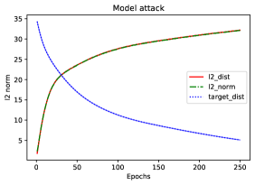
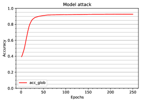
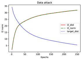
(a)    (b)  (c)    (d) 

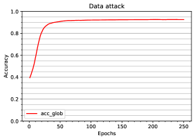
Figure 2: (2) Distance between $\rho^{t}$ and $\theta_{s}^{\dagger}$ (target_dist), under model attack (combining CGA and Proposition 4). (2) Accuracy of $\rho^{t}$ according to $\theta_{s}^{\dagger}$ (which relabels $0\rightarrow 1\rightarrow 2\rightarrow...\rightarrow 9\rightarrow 0$), under model attack (combining CGA and Proposition 4). (2) Distance between the global model $\rho^{t}$ and the target model $\theta_{s}^{\dagger}$ (target_dist), under our data poisoning attack. (2) Accuracy of $\rho^{t}$ according to $\theta_{s}^{\dagger}$ (which relabels $0\rightarrow 1\rightarrow 2\rightarrow...\rightarrow 9\rightarrow 0$), under our data poisoning attack.

5.2 From Gradient Attack to Model Attack Against $\ell_{2}^{2}$

We now show how to turn a gradient attack into model attack, against $\ell_{2}^{2}$ regularization. It is trivial to transform any gradient $g_{s}^{\infty}$ such that $\rho^{\infty}=\theta_{s}^{\dagger}$ into a model attack by setting $\theta_{s}^{\spadesuit}\triangleq\theta_{s}^{\dagger}-\frac{1}{2}g_{s}^{\infty}$, as guaranteed by the following result, and as depicted by Figure 2 and Figure 2.

Proposition 4.

Consider the $\ell_{2}^{2}$ regularization. Suppose that $g_{s}^{t}\rightarrow g_{s}^{\infty}$ and $\rho^{t}\rightarrow\theta_{s}^{\dagger}$, with a constant learning rate $\eta_{t}=\eta$. Then, under the model attack $\theta_{s}^{\spadesuit}\triangleq\theta_{s}^{\dagger}-\frac{1}{2\lambda}g_{s}^{\infty}$, the gradient at $\rho=\theta_{s}^{\dagger}$ vanishes, i.e. $\nabla_{\rho}\textsc{Loss}{}(\theta_{s}^{\dagger},\vec{\theta}^{*}_{-s}(\theta_{s}^{\dagger},\vec{\mathcal{D}}_{-s}),\theta_{s}^{\spadesuit},\mathcal{D}_{-s})=0$.

Proof.

Given a constant learning rate, the convergence $\rho^{t}\rightarrow\theta_{s}^{\dagger}$ implies that the sum of honest users’ gradients at $\rho=\theta_{s}^{\dagger}$ equals $-g_{s}^{\infty}$. Therefore, to achieve $\rho^{*}=\theta_{s}^{\dagger}$, it suffices to send $\theta_{s}^{\spadesuit}$ such that the gradient of $\lambda\left\lVert{\rho-\theta_{s}^{\spadesuit}}\right\rVert_{2}^{2}$ with respect to $\rho$ at $\rho=\theta_{s}^{\dagger}$ equals $g_{s}^{\infty}$. Since the gradient is $\lambda(\theta_{s}^{\dagger}-\theta_{s}^{\spadesuit})$, $\theta_{s}^{\spadesuit}\triangleq\theta_{s}^{\dagger}-\frac{1}{2\lambda}g_{s}^{\infty}$ does the trick. ∎

5.3 From Model Attack to Data Poisoning Against $\ell_{2}^{2}$

The case of linear regression.

In linear regression, any model attack can be turned into a single data poisoning attack, as proved by the following theorem whose proof is given in Appendix K.

Theorem 5.

Consider the $\ell_{2}^{2}$ regularization and linear regression. For any data $\mathcal{D}_{-s}$ and any target value $\theta_{s}^{\dagger}$, there is a datapoint $(\mathcal{Q},\mathcal{A})$ to be injected by user $s$ such that $\rho^{*}(\left\{(\mathcal{Q},\mathcal{A})\right\},\mathcal{D}_{-s})=\theta_{s}^{\dagger}$.

Sketch of proof.

We first identify the sum $g$ of honest users’ gradients, if the global model $\rho$ took the target value $\theta_{s}^{\dagger}$. We then determine the value $\theta_{s}^{\spadesuit}$ that the strategic user’s model must take, to counteract other users’ gradients. Reporting datapoint $(\mathcal{Q},\mathcal{A})\triangleq(g,g^{T}\theta_{s}^{\spadesuit}-1)$ then guarantees that the strategic user’s learned model will equal $\theta_{s}^{\spadesuit}$. ∎

Note that this single datapoint attack requires reporting a query $\mathcal{Q}$ whose norm grows as $\Theta(N)$, while the answer $\mathcal{A}$ grows as $\Theta(N^{2})$. Assuming a large number of users, this query will fall out of the distribution of users’ queries, and could thus be flagged by basic outlier detection techniques. We stress, however, that our proof can be trivially transformed into an attack with $\Theta(N^{2})$ data points, all of which have a query whose norm is $\mathcal{O}(1)$.

The case of linear classification.

We now consider linear classification, with the case of MNIST. By Lemma 2, any model attack can be turned into data poisoning, by (mis)labeling sufficiently many (random) data points, However, this may require creating too many data labelings, especially if the norm of $\theta_{s}^{\spadesuit}$ is large (which holds if $s$ faces many active users), as suggested by Theorem 3.

For efficient data poisoning, define the indifference affine subspace $V\subset\mathbb{R}^{d}$ as the set of images with equiprobable labels. Intuitively, labeling images close to $V$ is very informative, as it informs us directly about the separating hyperplanes. To generate images, we draw random images, project them orthogonally on $V$ and add a small noise. We then label the image probabilistically with model $\theta_{s}^{\spadesuit}$.

Figure 2 shows the effectiveness of the resulting data poisoning attack, with only 2,000 data points, as opposed to the 60,000 honestly labeled data points that the 10 other users cumulatively have. Remarkably, complete data relabeling was achieved by poisoning merely 3.3% of the total database. More details are given in Appendix L.

Note that this attack leads us to consider images not in $[0,1]^{d}$. In Appendix L.3, we report another equivalently effective attack, which only reports images in $[0,1]^{d}$, though it requires significantly more data injection.

5.4 Gradient Attack on Local Models

Note that CGA aims to merely bias the global model. However, the attacker may instead prefer to bias other users’ local models. To this end, we present here a variant of CGA, which targets the average of other users’ local models. At each iteration of this variant, the attacker reports

$$g_{s}^{t}\in\operatorname*{arg\,min}_{g\in\textsc{Grad}(\rho^{t})}\left\lVert{\rho^{t}-\eta_{t}(\hat{g}_{-s}^{t}+g)-\theta_{s}^{\dagger}-\frac{\hat{g}_{-s}^{t}}{2\lambda(N-1)}}\right\rVert_{2}.$$

Figure 3 shows the effectiveness of this attack. This gradient attack can evidently be turned into data poisoning similar to what was achieved for CGA.

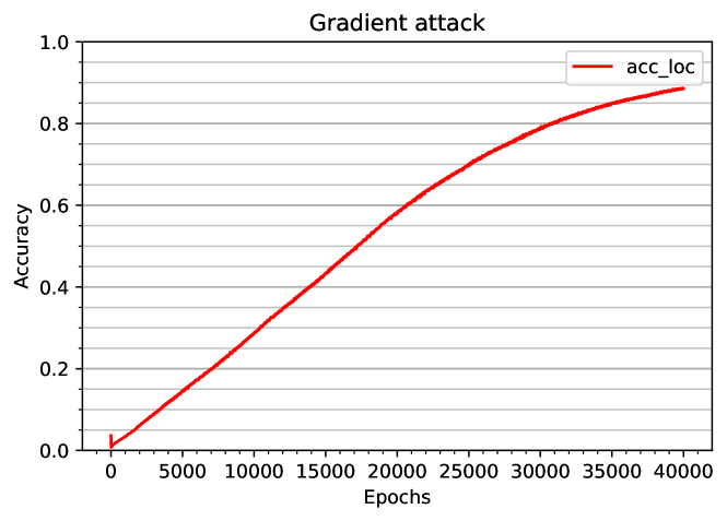
Figure 3: Accuracy of other users’ average local models according to $\theta_{s}^{\dagger}$ (which relabels $0\rightarrow 1\rightarrow 2\rightarrow...\rightarrow 9\rightarrow 0$), when attacked by CGA variant.

6 Conclusion

We showed that, unlike what has been argued, e.g., Shejwalkar et al. (2022), the gradient attack threat is not unrealistic. More precisely, for personalized federated learning with local PAC* guarantees, effective gradient attacks can be derived from strategic data reporting, with potentially surprisingly few data. In fact, by leveraging our newly found equivalence, we derived new impossibility theorems on what any robust learning algorithm can guarantee, under data poisoning attacks, especially, in highly-heterogeneous settings. Yet such attacks are known to be ubiquitous for high-risk applications, many of which are known to feature especially high heterogeneity, like online content recommendation. Arguably, a lot more security measures are urgently needed to make large-scale learning algorithms safe.

Ethics statement

The safety of algorithms is arguably a prerequisite to their ethics. After all, an arbitrarily manipulable large-scale algorithm will unavoidably endanger the targets of the entities that successfully design such algorithms. Typically, unsafe large-scale recommendation algorithms may be hacked by health disinformation campaigns that aim to promote non-certified products, e.g., by falsely pretending that they cure COVID-19. Such algorithms must not be regarded as ethical, even if they were designed with the best intentions. We believe that our work helps understand the vulnerabilities of such algorithms, and will motivate further research in the ethics and security of machine learning.

Appendix

Appendix A Convexity Lemmas

A.1 General Lemmas

Definition 4.

We say that $f:\mathbb{R}^{d}\rightarrow\mathbb{R}$ is locally strongly convex if, for any convex compact set $C\subset\mathbb{R}^{d}$, there exists $\mu>0$ such that $f$ is $\mu$-strongly convex on $C$, i.e. for any $x,y\in C$ and any $\lambda\in[0,1]$, we have

$$f(\lambda x+(1-\lambda)y)\leq\lambda f(x)+(1-\lambda)f(y)-\frac{\mu}{2}\lambda(1-\lambda)\left\lVert{x-y}\right\rVert_{2}^{2}.$$ (8)

It is well-known that if $f$ is differentiable, this condition amounts to saying that $\left\lVert{\nabla f(x)-\nabla f(y)}\right\rVert_{2}\geq\mu\left\lVert{x-y}\right\rVert_{2}$ for all $x,y\in C$. And if $f$ is twice differentiable, then it amounts to saying $\nabla^{2}f(x)\succeq\mu I$ for all $x\in C$.

Lemma 6.

If $f$ is locally strongly convex and $g$ is convex, then $f+g$ is locally strongly convex.

Proof.

Indeed, $(f+g)(\lambda x+(1-\lambda)y)\leq\lambda f(x)+(1-\lambda)f(y)-\frac{\mu}{2}\lambda(1-\lambda)\left\lVert{x-y}\right\rVert_{2}^{2}+\lambda g(x)+(1-\lambda)g(y)=\lambda(f+g)(x)+(1-\lambda)(f+g)(y)-\frac{\mu}{2}\lambda(1-\lambda)\left\lVert{x-y}\right\rVert_{2}^{2}$. ∎

Definition 5.

We say that $f:\mathbb{R}^{d}\rightarrow\mathbb{R}$ is $L$-smooth if it is differentiable and if its gradient is $L$-Lipschitz continuous, i.e. for any $x,y\in\mathbb{R}^{d}$,

$$\left\lVert{\nabla f(x)-\nabla f(y)}\right\rVert_{2}\leq L\left\lVert{x-y}\right\rVert_{2}.$$ (9)

Lemma 7.

If $f$ is $L_{f}$-smooth and $g$ is $L_{g}$-smooth, then $f+g$ is $(L_{f}+L_{g})$-smooth.

Proof.

Indeed, $\left\lVert{\nabla(f+g)(x)-\nabla(f+g)(y)}\right\rVert_{2}\leq\left\lVert{\nabla f(x)-\nabla f(y)}\right\rVert_{2}+\left\lVert{\nabla g(x)-\nabla g(y)}\right\rVert_{2}\leq L_{f}\left\lVert{x-y}\right\rVert_{2}+L_{g}\left\lVert{x-y}\right\rVert_{2}=(L_{f}+L_{g})\left\lVert{x-y}\right\rVert_{2}.$ ∎

Lemma 8.

Suppose that $f:\mathbb{R}^{d}\times\mathbb{R}^{d^{\prime}}\mapsto\mathbb{R}$ is locally strongly convex and $L$-smooth, and that, for any $x\in X$, where $X\subset\mathbb{R}^{d}$ is a convex compact subset, the map $y\mapsto f(x,y)$ has a minimum $y^{*}(x)$. Note that local strong convexity guarantees the uniqueness of this minimum. Then, there exists $K$ such that the function $y^{*}$ is $K$-Lipschitz continuous on $X$.

Proof.

The existence and uniqueness of $y^{*}(x)$ hold by strong convexity. Fix $x,x^{\prime}$. By optimality of $y^{*}$, we know that $\nabla_{y}f(x,y^{*}(x))=\nabla_{y}f(x^{\prime},y^{*}(x^{\prime}))=0$. We then have the following bounds

$$\mu\left\lVert{y^{*}(x)-y^{*}(x^{\prime})}\right\rVert_{2} \leq\left\lVert{\nabla_{y}f(x,y^{*}(x))-\nabla_{y}f(x,y^{*}(x^{\prime}))}\right\rVert_{2}=\left\lVert{\nabla_{y}f(x,y^{*}(x^{\prime}))}\right\rVert_{2}$$ (10)

$$=\left\lVert{\nabla_{y}f(x,y^{*}(x^{\prime}))-\nabla_{y}f(x^{\prime},y^{*}(x^{\prime}))}\right\rVert_{2}$$ (11)

$$\leq\left\lVert{\nabla f(x,y^{*}(x^{\prime}))-\nabla f(x^{\prime},y^{*}(x^{\prime}))}\right\rVert_{2}$$ (12)

$$\leq L\left\lVert{(x-x^{\prime},y^{*}(x^{\prime})-y^{*}(x^{\prime}))}\right\rVert_{2}=L\left\lVert{x-x^{\prime}}\right\rVert_{2},$$ (13)

where we first used the local strong convexity assumption, then the fact that $\nabla_{y}f(x,y^{*}(x))=0$, then the fact that $\nabla_{y}f(x^{\prime},y^{*}(x^{\prime}))=0$, and then the $L$-smooth assumption. ∎

Lemma 9.

Suppose that $f:\mathbb{R}^{d}\times\mathbb{R}^{d^{\prime}}\mapsto\mathbb{R}$ is locally strongly convex and $L$-smooth, and that, for any $x\in X$, where $X\subset\mathbb{R}^{d}$ is a convex compact subset, the map $y\mapsto f(x,y)$ has a minimum $y^{*}(x)$. Define $g(x)\triangleq\min_{y\in Y}f(x,y)$. Then $g$ is convex and differentiable on $X$ and $\nabla g(x)=\nabla_{x}f(x,y^{*}(x))$.

Proof.

First we prove that $g$ is convex. Let $x_{1},x_{2}\in\mathbb{R}^{d}$, and $\lambda_{1},\lambda_{2}\in[0,1]$ with $\lambda_{1}+\lambda_{2}=1$. For any $y_{1},y_{2}\in\mathbb{R}^{d^{\prime}}$, we have

$$g(\lambda_{1}x_{1}+\lambda_{2}x_{2}) =\min_{y\in\mathbb{R}^{d^{\prime}}}f(\lambda_{1}x_{1}+\lambda_{2}x_{2},y)$$ (14)

$$\leq f(\lambda_{1}x_{1}+\lambda_{2}x_{2},\lambda_{1}y_{1}+\lambda_{2}y_{2})$$ (15)

$$\leq\lambda_{1}f(x_{1},y_{1})+\lambda_{2}f(x_{2},y_{2}).$$ (16)

Taking the infimum of the right-hand side over $y_{1}$ and $y_{2}$ yields $g(\lambda_{1}x_{1}+\lambda_{2}x_{2})\leq\lambda_{1}g(x_{1})+\lambda_{2}g(x_{2})$, which proves the convexity of $g$.

Now denote $h(x)=\nabla_{x}f(x,y^{*}(x))$. We aim to show that $\nabla g(x)=h(x)$. Let $\varepsilon\in\mathbb{R}^{d}$ small enough so that $x+\varepsilon\in X$. Now note that we have

$$g(x+\varepsilon) =\min_{y\in\mathbb{R}^{d^{\prime}}}f(x+\varepsilon,y)\leq f(x+\varepsilon,y^{*}(x))$$ (17)

$$=f(x,y^{*}(x))+\varepsilon^{T}\nabla_{x}f(x,y^{*}(x))+o(\left\lVert{\varepsilon}\right\rVert_{2})$$ (18)

$$=g(x)+\varepsilon^{T}h(x)+o(\left\lVert{\varepsilon}\right\rVert_{2}),$$ (19)

which shows that $h(x)$ is a superderivative of $g$ at $x$. We now show that it is also a subderivative. To do so, first note that its value at $x+\varepsilon$ is approximately the same, i.e.

$$\left\lVert{h(x+\varepsilon)-h(x)}\right\rVert_{2} \leq\left\lVert{\nabla_{x}f(x+\varepsilon,y^{*}(x+\varepsilon))-\nabla_{x}f(x,y^{*}(x+\varepsilon))}\right\rVert_{2}$$

$$\qquad\qquad\qquad+\left\lVert{\nabla_{x}f(x,y^{*}(x+\varepsilon))-\nabla_{x}f(x,y^{*}(x))}\right\rVert_{2}$$ (20)

$$\leq L\left\lVert{\varepsilon}\right\rVert_{2}+L\left\lVert{y^{*}(x+\varepsilon)-y^{*}(x)}\right\rVert_{2}\leq\left(L+\frac{L^{2}}{\mu}\right)\left\lVert{\varepsilon}\right\rVert_{2},$$ (21)

where we used the $L$-smoothness of $f$ and Lemma 8. Now notice that

$$g(x) =\min_{y\in\mathbb{R}^{d^{\prime}}}f(x,y)\leq f(x,y^{*}(x+\varepsilon))=f((x+\varepsilon)-\varepsilon,y^{*}(x+\varepsilon))$$ (22)

$$=f(x+\varepsilon,y^{*}(x+\varepsilon))-\varepsilon^{T}\nabla_{x}f(x+\varepsilon,y^{*}(x+\varepsilon))+o(\left\lVert{\varepsilon}\right\rVert_{2})$$ (23)

$$=g(x+\varepsilon)-\varepsilon^{T}h(x)-\varepsilon^{T}\left(h(x+\varepsilon)-h(x)\right)+o(\left\lVert{\varepsilon}\right\rVert_{2}),$$ (24)

But we know that $\left\lVert{h(x+\varepsilon)-h(x)}\right\rVert_{2}=\mathcal{O}(\left\lVert{\varepsilon}\right\rVert_{2})$. Rearranging the terms then yields

$$g(x+\varepsilon)\geq g(x)+\varepsilon^{T}h(x)-o(\left\lVert{\varepsilon}\right\rVert_{2}),$$ (25)

which shows that $h(x)$ is also a subderivative. Therefore, we know that $g(x+\varepsilon)=g(x)+\varepsilon^{T}h(x)+o(\left\lVert{\varepsilon}\right\rVert_{2})$, which boils down to saying that $g$ is differentiable in $x\in X$, and that $\nabla g(x)=h(x)$. ∎

Lemma 10.

Suppose that $f:X\times\mathbb{R}^{d^{\prime}}\rightarrow\mathbb{R}$ is $\mu$-strongly convex, where $X\subset\mathbb{R}^{d}$ is closed and convex. Then $g:X\rightarrow\mathbb{R}$, defined by $g(x)=\inf_{y\in Y}f(x,y)$, is well-defined and $\mu$-strongly convex too.

Proof.

The function $y\mapsto f(x,y)$ is still strongly convex, which means that it is at least equal to a quadratic approximation around 0, which is a function that goes to infinity in all directions as $\left\lVert{y}\right\rVert_{2}\rightarrow\infty$. This proves that the infimum must be reached within a compact set, which implies the existence of a minimum. Thus $g$ is well-defined. Moreover, for any $x_{1},x_{2}\in X,y_{1},y_{2}\in\mathbb{R}^{d^{\prime}}$, and $\lambda_{1},\lambda_{2}\geq 0$ with $\lambda_{1}+\lambda_{2}=1$, we have

$$g(\lambda_{1}x_{1}+\lambda_{2}x_{2}) =\inf_{y}f(\lambda_{1}x_{1}+\lambda_{2}x_{2},y)$$ (26)

$$\leq f(\lambda_{1}x_{1}+\lambda_{2}x_{2},\lambda_{1}y_{1}+\lambda_{2}y_{2})$$ (27)

$$\leq\lambda_{1}f(x_{1},y_{1})+\lambda_{2}f(x_{2},y_{2})-\frac{\mu}{2}\lambda_{1}\lambda_{2}\left\lVert{(x_{1}-x_{2},y_{1}-y_{2})}\right\rVert_{2}^{2}$$ (28)

$$\leq\lambda_{1}f(x_{1},y_{1})+\lambda_{2}f(x_{2},y_{2})-\frac{\mu}{2}\lambda_{1}\lambda_{2}\left\lVert{x_{1}-x_{2}}\right\rVert_{2}^{2},$$ (29)

where we used the $\mu$-strong convexity of $f$. Taking the infimum over $y_{1},y_{2}$ implies the $\mu$-strong convexity of $g$. ∎

A.2 Applications to Loss

Now instead of proving our theorems for different cases separately, we make the following assumptions on the components of the global loss that encompasses both $\ell_{2}^{2}$ and smooth-$\ell_{2}$ regularization, a well as linear regression and logistic regression.

Assumption 1.

Assume that $\ell$ is convex and $L_{\ell}$-smooth, and that $\mathcal{R}(\rho,\theta)=\mathcal{R}_{0}(\rho-\theta)$, where $\mathcal{R}_{0}:\mathbb{R}^{d}\rightarrow\mathbb{R}$ is locally strongly convex (i.e. strongly convex on any convex compact set), $L_{\mathcal{R}_{0}}$-smooth and satisfy $\mathcal{R}_{0}(z)=\Omega(\left\lVert{z}\right\rVert_{2})$ as $\left\lVert{z}\right\rVert_{2}\rightarrow\infty$.

Lemma 11.

Under Assumption 1, Loss is locally strongly convex and $L$-smooth.

Proof.

All terms of Loss are $L_{0}$-smooth, for an appropriate value of $L_{0}$. By Lemma 7, their sum is thus also $L$-smooth, for an appropriate value of $L$. Now, given Lemma 6, to prove that Loss is locally strongly convex, it suffices to prove that $\nu\sum\left\lVert{\theta_{n}}\right\rVert_{2}^{2}+\mathcal{R}_{0}(\rho-\theta_{1})$ is locally strongly convex. Consider any convex compact set $C\subset\mathbb{R}^{d\times(1+N)}$. Since $\mathcal{R}_{0}$ is locally strongly convex, we know that there exists $\mu>0$ such that $\nabla^{2}\mathcal{R}_{0}\succeq\mu I$. As a result,

$$(\rho,\vec{\theta}{})^{T} \left(\nabla^{2}\textsc{Loss}{}\right)(\rho,\vec{\theta}{})\geq\nu\sum_{n\in[N]}\left\lVert{\theta_{n}}\right\rVert_{2}^{2}+\mu\left\lVert{\rho-\theta_{1}}\right\rVert_{2}^{2}$$ (30)

$$=\nu\left\lVert{\theta_{1}}\right\rVert_{2}^{2}+\mu\left\lVert{\rho}\right\rVert_{2}^{2}+\mu\left\lVert{\theta_{1}}\right\rVert_{2}^{2}-2\mu\rho^{T}\theta_{1}+\nu\sum_{n\neq 1}\left\lVert{\theta_{n}}\right\rVert_{2}^{2}.$$ (31)

Now define $\alpha\triangleq\sqrt{\frac{2\mu}{\nu+2\mu}}$. Clearly, $0<\alpha<1$. Moreover, $0\leq\left\lVert{\frac{1}{\alpha}\theta_{1}-\alpha\rho}\right\rVert_{2}^{2}=\frac{1}{\alpha^{2}}\left\lVert{\theta_{1}}\right\rVert_{2}^{2}+\alpha^{2}\left\lVert{\rho}\right\rVert_{2}^{2}-2\rho^{T}\theta_{1}$. Therefore $2\rho^{T}\theta_{1}\leq\alpha^{2}\left\lVert{\rho}\right\rVert_{2}^{2}+\frac{1}{\alpha^{2}}\left\lVert{\theta_{1}}\right\rVert_{2}^{2}$, which thus implies

$$(\rho,\vec{\theta}{})^{T} \left(\nabla^{2}\textsc{Loss}{}\right)(\rho,\vec{\theta}{})\geq\left(\nu+\mu\left(1-\alpha^{-2}\right)\right)\left\lVert{\theta_{1}}\right\rVert_{2}^{2}+\mu\left(1-\alpha^{2}\right)\left\lVert{\rho}\right\rVert_{2}^{2}+\nu\sum_{n\neq 1}\left\lVert{\theta_{n}}\right\rVert_{2}^{2}$$ (32)

$$\geq\frac{\nu}{2}\left\lVert{\theta_{1}}\right\rVert_{2}^{2}+\frac{2\nu\mu}{\nu+2\mu}\left\lVert{\rho}\right\rVert_{2}^{2}+\nu\sum_{n\neq 1}\left\lVert{\theta_{n}}\right\rVert_{2}^{2}\geq\min\left\{\frac{\nu}{2},\frac{2\nu\mu}{\nu+2\mu}\right\}\left\lVert{(\rho,\vec{\theta}{})}\right\rVert_{2}^{2},$$ (33)

which proves that $\nabla^{2}\textsc{Loss}{}\succeq\kappa I$, with $\kappa>0$. This shows that Loss is locally strongly convex. ∎

Lemma 12.

Under Assumption 1, $\rho\mapsto\vec{\theta}^{*}{}(\rho,\vec{\mathcal{D}})$ is Lipchitz continuous on any compact set.

Proof.

Define $f_{n}(\rho,\theta_{n})\triangleq\nu\left\lVert{\theta_{n}}\right\rVert_{2}^{2}+\sum_{x\in\mathcal{D}_{n}}\ell(\theta_{n},x)+\lambda\left\lVert{\rho-\theta_{n}}\right\rVert_{2}^{2}$. If $\ell$ is $L$-smooth, then $f_{n}$ is clearly $(\left\lvert{\mathcal{D}_{n}}\right\rvert L+\nu+\lambda)$-smooth. Moreover, if $\ell$ is convex, then for any $\rho$, the function $\theta_{n}\mapsto f_{n}(\rho,\theta_{n})$ is at least $\nu$-strongly convex. Thus Lemma 8 applies, which guarantees that $\rho\mapsto\vec{\theta}^{*}{}(\rho,\vec{\mathcal{D}})$ is Lipchitz. ∎

Lemma 13.

Under Assumption 1, $\rho\mapsto\textsc{Loss}{}(\rho,\vec{\theta}^{*}(\rho,\vec{\mathcal{D}}),\vec{\mathcal{D}})$ is $L$-smooth and locally strongly convex.

Proof.

By Lemma 11, the global loss is known to be $L$-smooth, for some value of $L$ and locally strongly convex. Denoting $f:\rho\mapsto\textsc{Loss}{}(\rho,\vec{\theta}^{*}(\rho,\vec{\mathcal{D}}),\vec{\mathcal{D}})$, we then have

$$\left\lVert{\nabla f(\rho)-\nabla f(\rho^{\prime})}\right\rVert_{2} \leq\left\lVert{\nabla_{\rho}\textsc{Loss}{}(\rho,\vec{\theta}^{*}(\rho,\vec{\mathcal{D}}),\vec{\mathcal{D}})-\nabla_{\rho}\textsc{Loss}{}(\rho^{\prime},\vec{\theta}^{*}(\rho^{\prime},\vec{\mathcal{D}}),\vec{\mathcal{D}})}\right\rVert_{2}$$ (34)

$$\leq L\left\lVert{(\rho,\vec{\theta}^{*}(\rho,\vec{\mathcal{D}}))-(\rho^{\prime},\vec{\theta}^{*}(\rho^{\prime},\vec{\mathcal{D}}))}\right\rVert_{2}$$ (35)

$$\leq L\left\lVert{\rho-\rho^{\prime}}\right\rVert_{2},$$ (36)

which proves that $f$ is $L$-smooth.

For strong convexity, note that since the global loss function is locally strongly convex, for any compact convex set $C$, there exists $\mu$ such that $\textsc{Loss}{}(\rho,\vec{\theta}{},\vec{\mathcal{D}})$ is $\mu$-strongly convex on $C=(C_{1},C_{2})\subset(\mathbb{R}^{d},\mathbb{R}^{N\times d})$, therefore, by Lemma 10, $f(\rho)$ will also be $\mu$-strongly convex on $C_{1}$ which means that $f(\rho)$ is locally strongly convex. ∎

Appendix B Proof of the Equivalence

B.1 Proof of the Reduction from Model Attack to Data Poisoning

Proof of Lemma 1.

We omit making the dependence of the optima on $\vec{\mathcal{D}}$ explicit, and we consider any other models $\rho$ and $\vec{\theta}_{-s}$. We have the following inequalities:

$$\textsc{Loss}_{s} (\rho^{*},\vec{\theta}^{*}_{-s},\theta_{s}^{\spadesuit},\vec{\mathcal{D}})=\textsc{Loss}{}(\rho^{*},\vec{\theta}^{*}{},\vec{\mathcal{D}})-\mathcal{L}(\theta_{s}^{*},\mathcal{D}_{s})$$ (37)

$$\leq\textsc{Loss}{}(\rho,(\vec{\theta}_{-s},\theta_{s}^{*}),\vec{\mathcal{D}})-\mathcal{L}(\theta_{s}^{*},\mathcal{D}_{s})=\textsc{Loss}_{s}(\rho,\vec{\theta}_{-s},\theta_{s}^{\spadesuit},\vec{\mathcal{D}}),$$ (38)

where we used the optimality of $(\rho^{*},\vec{\theta}^{*}{})$ in the second line, and where we repeatedly used the fact that $\theta_{s}^{*}=\theta_{s}^{\spadesuit}$. This proves that $(\rho^{*},\vec{\theta}^{*}_{-s})$ is a global minimum of the modified loss. ∎

B.2 Proof of the Reduction from Data Poisoning to Model Attack

First, we define the following modified loss function:

$$\textsc{Loss}_{s}(\rho,\vec{\theta}_{-s},\theta_{s}^{\spadesuit},\vec{\mathcal{D}}_{-s})\triangleq\textsc{Loss}{}(\rho,(\theta_{s}^{\spadesuit},\vec{\theta}_{-s}),(\emptyset,\vec{\mathcal{D}}_{-s}))$$ (39)

where $\vec{\theta}_{-s}$ and $\vec{\mathcal{D}}_{-s}$ are variables and datasets for users $n\neq s$. We then define $\rho^{*}{}(\theta_{s}^{\spadesuit},\vec{\mathcal{D}}_{-s})$ and $\vec{\theta}^{*}_{-s}(\theta_{s}^{\spadesuit},\vec{\mathcal{D}}_{-s})$ as a minimum of the modified loss function, and $\theta_{s}^{*}(\theta_{s}^{\spadesuit},\vec{\mathcal{D}}_{-s})\triangleq\theta_{s}^{\spadesuit}$. We now prove a slightly more general version of Lemma 2, which applies to a larger class of regularizations. It also shows how to construct the strategic’s user data poisoning attack.

Lemma 14 (Reduction from data poisoning to model attack).

Assume local PAC* learning. Suppose also that $\mathcal{R}$ is continuous and that $\mathcal{R}(\rho,\theta)\rightarrow\infty$ when $\left\lVert{\rho-\theta}\right\rVert_{2}\rightarrow\infty$. Consider any datasets $\mathcal{D}_{-s}$ and any attack model $\theta_{s}^{\spadesuit}$ such that the modified loss $\textsc{Loss}_{s}$ has a unique minimum $\rho^{*}(\theta_{s}^{\spadesuit},\vec{\mathcal{D}}_{-s}),\vec{\theta}^{*}_{-s}(\theta_{s}^{\spadesuit},\vec{\mathcal{D}}_{-s})$. Then, for any $\varepsilon,\delta>0$, there exists $\mathcal{I}$ such that if user $s$’s dataset $\mathcal{D}_{s}$ contains at least $\mathcal{I}$ inputs drawn from model $\theta_{s}^{\spadesuit}$, then, with probability at least $1-\delta$, we have

$$\left\lVert{\rho^{*}{}(\vec{\mathcal{D}})-\rho^{*}{}(\theta_{s}^{\spadesuit},\vec{\mathcal{D}}_{-s})}\right\rVert_{2}\leq\varepsilon~{}~{}\text{and}~{}~{}\forall n\neq s,~{}\left\lVert{\theta_{n}^{*}(\vec{\mathcal{D}})-\theta_{n}^{*}(\theta_{s}^{\spadesuit},\vec{\mathcal{D}}_{-s})}\right\rVert_{2}\leq\varepsilon.$$ (40)

Clearly, $\ell_{2}^{2}$, $\ell_{2}$ and smooth-$\ell_{2}$ are continuous regularizations, and verify $\mathcal{R}(\rho,\theta)\rightarrow\infty$ when $\left\lVert{\rho-\theta}\right\rVert_{2}\rightarrow\infty$. Moreover, setting $\delta\triangleq 1/2$ shows that the probability that the dataset $\mathcal{D}_{s}$ satisfies the inequalities of Lemma 14 is positive. This implies in particular that there must be a dataset $\mathcal{D}_{s}$ that satisfies these inequalities. All in all, this shows that Lemma 14 implies Lemma 2.

Proof of Lemma 14.

Let $\varepsilon,\delta> 0$ and $\theta_{s}^{\spadesuit}\in\mathbb{R}^{d}$. Denote $\rho^{\spadesuit}\triangleq\rho^{*}(\theta_{s}^{\spadesuit},\vec{\mathcal{D}}_{-s})$ and $\vec{\theta}^{\spadesuit}\triangleq\vec{\theta}^{*}(\theta_{s}^{\spadesuit},\vec{\mathcal{D}}_{-s})$ the result of strategic user $s$’s model attack. We define the compact set $C$ by

$$C\triangleq\left\{\rho,\vec{\theta}_{-s}\,\middle|\,\left\lVert{\rho{}-\rho^{\spadesuit}}\right\rVert_{2}\leq\varepsilon\wedge\forall n\neq s,~{}\left\lVert{\theta_{n}-\theta_{n}^{\spadesuit}}\right\rVert_{2}\leq\varepsilon\right\}$$ (41)

We define $D\triangleq\overline{\mathbb{R}^{d\times N}-C}$ the closure of the complement of $C$. Clearly, $\rho^{\spadesuit},\vec{\theta}_{-s}^{\spadesuit}\notin D$. We aim to show that, when strategic user $s$ reveals a large dataset $\mathcal{D}_{s}$ whose answers are provided using the attack model $\theta_{s}^{\spadesuit}$, then the same holds for any global minimum of the global loss $\rho^{*}{}(\vec{\mathcal{D}}),\vec{\theta}^{*}_{-s}(\vec{\mathcal{D}})\in C$. Note that, to prove this, it suffices to prove that the modified loss takes too large values, even when $\theta_{s}^{\spadesuit}$ is replaced by $\theta_{s}^{*}(\vec{\mathcal{D}})$.

Let us now formalize this. Denote $L^{\spadesuit}\triangleq\textsc{Loss}_{s}(\rho^{\spadesuit},\vec{\theta}_{-s}^{\spadesuit},\theta_{s}^{\spadesuit},\vec{\mathcal{D}}_{-s})$. We define

$$\eta\triangleq\inf_{\rho,\vec{\theta}_{-s}\in D}\textsc{Loss}_{s}(\rho,\vec{\theta}_{-s},\theta_{s}^{\spadesuit},\vec{\mathcal{D}}_{-s})-L^{\spadesuit}.$$ (42)

By a similar argument as that of Lemma 5, using the assumption $\mathcal{R}\rightarrow\infty$ at infinity, we know that the infimum is actually a minimum. Moreover, given that the minimum of the modified loss $\textsc{Loss}_{s}$ is unique, we know that the value of the loss function at this minimum is different from its value at $\rho^{\spadesuit},\vec{\theta}_{-s}^{\spadesuit}$. As a result, we must have $\eta>0$.

Now, since the function $\mathcal{R}$ is differentiable, it must be continuous. By the Heine–Cantor theorem, it is thus uniformly continuous on all compact sets. Thus, there must exist $\kappa> 0$ such that, for all models $\theta_{s}$ satisfying $\left\lVert{\theta_{s}-\theta_{s}^{\spadesuit}}\right\rVert_{2}\leq\kappa$, we have

$$\left\lvert{\mathcal{R}(\theta_{s},\rho^{\spadesuit})-\mathcal{R}(\theta_{s}^{\spadesuit},\rho^{\spadesuit})}\right\rvert\leq\eta/3.$$ (43)

Now, Lemma 5 guarantees the existence of $\mathcal{I}$ such that, if user $s$ provides a dataset $\mathcal{D}_{s}$ of least $\mathcal{I}$ answers with the model $\theta_{s}^{\spadesuit}$, then with probability at least $1-\delta$, we will have $\left\lVert{\theta_{s}^{*}(\vec{\mathcal{D}})-\theta_{s}^{\spadesuit}}\right\rVert_{2}\leq\min(\kappa,\varepsilon)$. Under this event, we then have

$$\textsc{Loss}_{s}\left(\rho^{\spadesuit},\vec{\theta}_{-s}^{\spadesuit},\theta_{s}^{*}(\vec{\mathcal{D}}),\vec{\mathcal{D}}_{-s}\right)\leq L^{\spadesuit}+\eta/3.$$ (44)

Then

$$\inf_{\rho,\vec{\theta}_{-s}\in D} \textsc{Loss}_{s}(\rho,\vec{\theta}_{-s},\theta_{s}^{*}(\vec{\mathcal{D}}),\vec{\mathcal{D}}_{-s})\geq\inf_{\rho,\vec{\theta}_{-s}\in D}\textsc{Loss}_{s}(\rho,\vec{\theta}_{-s},\theta_{s}^{\spadesuit},\vec{\mathcal{D}}_{-s})-\eta/3$$ (45)

$$\geq L^{\spadesuit}+\eta-\eta/3\geq L^{\spadesuit}+2\eta/3$$ (46)

$$>\textsc{Loss}_{s}\left(\rho^{\spadesuit},\vec{\theta}_{-s}^{\spadesuit},\theta_{s}^{*}(\vec{\mathcal{D}}),\vec{\mathcal{D}}_{-s}\right).$$ (47)

This shows that there is a high probability event under which the minimum of $\rho,\vec{\theta}_{-s}\mapsto\textsc{Loss}_{s}\left(\rho,\vec{\theta}_{-s},\theta_{s}^{*}(\vec{\mathcal{D}}),\vec{\mathcal{D}}_{-s}\right)$ cannot be reached in $D$. This is equivalent to what the theorem we needed to prove states. ∎

B.3 Proof of Reduction from Model Attack to Gradient Attack

Proof of Lemma 3.

We define

$$\textsc{Loss}^{1}_{s}(\rho) \triangleq\inf_{\vec{\theta}_{-s}}\left\{\textsc{Loss}{}(\rho,\vec{\theta}{},\vec{\mathcal{D}})-\mathcal{L}_{s}(\theta_{s},\mathcal{D}_{s})-\mathcal{R}(\rho,\theta_{s})\right\}+\rho^{T}g_{s}^{\infty}$$ (48)

$$=\inf_{\vec{\theta}_{-s}}\left\{\sum_{n\neq s}\mathcal{L}_{n}(\theta_{n},\mathcal{D}_{n})+\sum_{n\neq s}\mathcal{R}(\rho,\theta_{n})\right\}+\rho^{T}g_{s}^{\infty},$$ (49)

By Lemma 13, we know that $\textsc{Loss}^{1}_{s}(\rho)$ is locally strongly convex and has a unique minimum. By the definition of $\rho^{\infty}$, we must have $\sum_{n\neq s}\nabla_{\rho}\mathcal{R}(\rho^{\infty},\theta_{n}^{*}(\rho^{\infty}))+g_{s}^{\infty}=0$, and thus $\nabla_{\rho}\textsc{Loss}^{1}_{s}(\rho^{\infty})=0$. Now define

$$\textsc{Loss}^{2}_{s}(\rho,\theta_{s}) \triangleq\inf_{\vec{\theta}_{-s}}\left\{\textsc{Loss}{}(\rho,\vec{\theta}{},\vec{\mathcal{D}})-\mathcal{L}_{s}(\theta_{s},\mathcal{D}_{s})\right\}$$ (50)

$$=\textsc{Loss}^{1}_{s}(\rho)+\mathcal{R}(\rho,\theta_{s})-\rho^{T}g_{s}^{\infty},$$ (51)

and $\rho^{*}(\theta_{s})$, its minimizer. Therefore, we have

$$\nabla_{\rho}\textsc{Loss}^{2}_{s}(\rho,\theta_{s})=\nabla_{\rho}\textsc{Loss}^{1}_{s}(\rho)+\nabla_{\rho}\mathcal{R}(\rho,\theta_{s})-g_{s}^{\infty}.$$ (52)

By Lemma 13, we know that $\textsc{Loss}^{2}_{s}$ is locally strongly convex. Therefore, there exists $\mu_{1}>0$ such that $\textsc{Loss}^{2}_{s}(\rho,\theta_{s})$ is $\mu_{1}$-strongly convex in $\left\{(\theta_{s},\rho):\left\lVert{\nabla_{\rho}\mathcal{R}(\rho^{\infty},\theta_{s})-g_{s}^{\infty}}\right\rVert_{2}\leq\ \varepsilon_{2},\left\lVert{\rho-\rho^{*}(\theta_{s})}\right\rVert_{2}\leq 1\right\}$ for $\varepsilon_{2}$ small enough. Therefore, since $\nabla_{\rho}\textsc{Loss}^{2}_{s}(\rho^{*}(\theta_{s}),\theta_{s})=0$, for any $0<\varepsilon<1$, if $\left\lVert{\rho^{\infty}-\rho^{*}(\theta_{s})}\right\rVert_{2}>\varepsilon$, we then have

$$\varepsilon\left\lVert{\nabla_{\rho}\textsc{Loss}^{2}_{s}(\rho^{\infty},\theta_{s})}\right\rVert_{2} \geq(\rho^{\infty}-\rho^{*}(\theta_{s}))^{T}\nabla_{\rho}\textsc{Loss}^{2}_{s}(\rho^{\infty},\theta_{s})$$ (53)

$$\geq{\mu_{1}}\left\lVert{\rho^{\infty}-\rho^{*}(\theta_{s})}\right\rVert_{2}^{2}\geq\mu_{1}\varepsilon^{2},$$ (54)

and thus $\left\lVert{\nabla_{\rho}\textsc{Loss}^{2}_{s}(\rho^{\infty},\theta_{s})}\right\rVert_{2}\geq\mu_{1}\varepsilon$.

Now since $g_{s}^{\infty}\in\textsc{Grad}(\rho^{\infty})$ there exists $\theta_{s}^{\spadesuit}\in\mathbb{R}^{d}$ such that $\left\lVert{\nabla_{\rho}\mathcal{R}(\rho^{\infty},\theta_{s}^{\spadesuit})-g_{s}^{\infty}}\right\rVert_{2}\leq\min\left\{\varepsilon_{2},\frac{\mu_{1}\varepsilon}{2}\right\}$ which yields

$$\left\lVert{\nabla_{\rho}\textsc{Loss}^{2}_{s}(\rho^{\infty},\theta_{s}^{\spadesuit})}\right\rVert_{2} =\left\lVert{\nabla_{\rho}\textsc{Loss}^{1}_{s}(\rho^{\infty})+\nabla_{\rho}\mathcal{R}(\rho^{\infty},\theta_{s}^{\spadesuit})-g_{s}^{\infty}}\right\rVert_{2}$$ (55)

$$=\left\lVert{\nabla_{\rho}\mathcal{R}(\rho^{\infty},\theta_{s}^{\spadesuit})-g_{s}^{\infty}}\right\rVert_{2}\leq\frac{\mu_{1}\varepsilon}{2},$$ (56)

which contradicts (54) if $\left\lVert{\rho^{\infty}-\rho^{*}(\theta_{s}^{\spadesuit})}\right\rVert_{2}>\varepsilon$. Therefore, we must have $\left\lVert{\rho^{\infty}-\rho^{*}{}(\theta_{s}^{\spadesuit},\vec{\mathcal{D}}_{-s})}\right\rVert_{2}\leq\varepsilon$.

∎

Appendix C Proof of Convergence for the Global Model

In this section, we prove a slightly more general result than Proposition 1. Namely, instead of working with specific regularizations, we consider a more general class of regularizations, identified by Assumption 1.

Lemma 15.

Suppose Assumption 1 holds true. Assume that $\mathcal{L}_{n}$ is convex and $L$-smooth for all users $n\in[N]$. If $g_{s}^{t}$ converges and if $\eta_{t}=\eta$ is a constant small enough, then $\rho^{t}$ will converge too.

Note that since $\ell_{2}^{2}$ and smooth-$\ell_{2}$ regularizations satisfy Assumption 1, Lemma 15 clearly implies Proposition 1. We now introduce the key objects of the proof of Lemma 15.

Denote $g_{s}^{\infty}$ the limit of the attack gradients $g_{s}^{t}$. We now define

$$\textsc{Loss}^{1}_{s}(\rho) \triangleq\inf_{\vec{\theta}_{-s}}\left\{\textsc{Loss}{}(\rho,\vec{\theta}{},\vec{\mathcal{D}})-\mathcal{L}_{s}(\theta_{s},\mathcal{D}_{s})-\mathcal{R}(\rho,\theta_{s})\right\}+\rho^{T}g_{s}^{\infty}$$ (57)

$$=\inf_{\vec{\theta}_{-s}}\left\{\sum_{n\neq s}\mathcal{L}_{n}(\theta_{n},\mathcal{D}_{n})+\sum_{n\neq s}\mathcal{R}(\rho,\theta_{n})\right\}+\rho^{T}g_{s}^{\infty},$$ (58)

and prove that $\rho^{t}$ will converge to the minimizer of $\textsc{Loss}^{1}_{s}(\rho)$. By Lemma 13, we know that $\textsc{Loss}^{1}_{s}(\rho)$ is both locally strongly convex and $L$-smooth.

Now define $\zeta_{s}^{t}\triangleq g_{s}^{t}-g_{s}^{\infty}$. We then have $\zeta_{s}^{t}\rightarrow 0$ and $\nabla\textsc{Loss}^{1}_{s}(\rho^{t})$ is the sum of all gradient vectors received from all users assuming the strategic user $s$ sends the vector $g_{s}^{\infty}$ in all iterations. Thus, at iteration $t$ of the optimization algorithm, we will take one step in the direction $G^{t}\triangleq\nabla\textsc{Loss}^{1}_{s}(\rho^{t})+\zeta_{s}^{t}$, i.e.,

$$\rho^{t+1}=\rho^{t}-\eta_{t}G^{t}.$$ (59)

We now prove the following lemma that bounds the difference between the function value in two successive iterations.

Lemma 16.

If $\textsc{Loss}^{1}_{s}(\rho)$ is $L$-smooth and $\eta_{t}\leq 1/L$, we have

$$\textsc{Loss}^{1}_{s}(\rho^{t+1})-\textsc{Loss}^{1}_{s}(\rho^{t})\leq-\frac{\eta_{t}}{2}\left\lVert{G^{t}}\right\rVert_{2}^{2}+\eta_{t}{\zeta_{s}^{t}}^{T}G^{t}.$$ (60)

Proof.

Since $\textsc{Loss}^{1}_{s}$ is $L$-smooth, we have

$$\textsc{Loss}^{1}_{s}(\rho^{t+1})\leq\textsc{Loss}^{1}_{s}(\rho^{t})+(\rho^{t+1}-\rho^{t})^{T}\nabla\textsc{Loss}^{1}_{s}(\rho^{t})+\frac{L}{2}\left\lVert{\rho^{t+1}-\rho^{t}}\right\rVert_{2}^{2}.$$ (61)

Now plugging $\rho^{t+1}-\rho^{t}=-\eta_{t}G^{t}$ and $\nabla\textsc{Loss}^{1}_{s}(\rho^{t})=G^{t}-\zeta_{s}^{t}$ into the inequality implies

$$\textsc{Loss}^{1}_{s}(\rho^{t+1})-\textsc{Loss}^{1}_{s}(\rho^{t}) \leq\left(-\eta_{t}G^{t}\right)^{T}\left(G^{t}-\zeta_{s}^{t}\right)+\frac{L}{2}\left\lVert{-\eta_{t}G^{t}}\right\rVert_{2}^{2}$$ (62)

$$\leq-\frac{\eta_{t}}{2}\left\lVert{G^{t}}\right\rVert_{2}^{2}+\eta_{t}{\zeta_{s}^{t}}^{T}G^{t},$$ (63)

where we used the fact $\eta_{t}\leq 1/L$. ∎

C.0.1 The global model remains bounded

Lemma 17.

There is $M$ such that, for all $t$, $\textsc{Loss}^{1}_{s}(\rho^{t})\leq M$.

Proof.

Consider the closed ball $\mathcal{B}(\rho^{*},1)$ centered on $\rho^{*}$ and of radius 1. By Lemma 13, we know that $\textsc{Loss}^{1}_{s}$ is locally strongly convex and thus there exists a $\mu_{1}>0$ such that $\textsc{Loss}^{1}_{s}$ is $\mu_{1}$-strongly convex on $\mathcal{B}(\rho^{*},1)$. Now consider a point $\rho_{1}$ on the boundary of $\mathcal{B}(\rho^{*},1)$. By strong convexity we have

$$\left\lVert{\nabla\textsc{Loss}^{1}_{s}(\rho_{1})}\right\rVert_{2}^{2}\geq(\rho_{1}-\rho^{*})^{T}\nabla\textsc{Loss}^{1}_{s}(\rho_{1})\geq{\mu_{1}}\left\lVert{\rho_{1}-\rho^{*}}\right\rVert_{2}^{2}={\mu_{1}}.$$ (64)

Now similarly, by the convexity of $\textsc{Loss}^{1}_{s}$ on $\mathbb{R}^{d}$, for any $\rho\in\mathbb{R}^{d}-\mathcal{B}(\rho^{*},1)$, we have $\left\lVert{\nabla\textsc{Loss}^{1}_{s}(\rho_{1})}\right\rVert_{2}\geq\sqrt{{\mu_{1}}}$. Now since $\zeta_{s}^{t}\rightarrow 0$, there exists an iteration $T_{1}$ after which ($t\geq T_{1}$), we have $\left\lVert{\zeta_{s}^{t}}\right\rVert_{2}\leq\frac{1}{4}\sqrt{{\mu_{1}}}$, and thus $\left\lVert{G^{t}}\right\rVert_{2}\geq\left\lVert{\nabla\textsc{Loss}^{1}_{s}(\rho^{t})}\right\rVert_{2}-\left\lVert{\zeta_{s}^{t}}\right\rVert_{2}\geq\frac{3}{4}\sqrt{{\mu_{1}}}$. Thus, Lemma 16 implies that for $t\geq T_{1}$, if $\left\lVert{\rho^{t}-\rho^{*}}\right\rVert_{2}\geq 1$, then

$$\textsc{Loss}^{1}_{s}(\rho^{t+1})-\textsc{Loss}^{1}_{s}(\rho^{t}) \leq-\frac{\eta}{2}\left\lVert{G^{t}}\right\rVert_{2}^{2}+\eta{\zeta_{s}^{t}}^{T}G^{t}$$ (65)

$$\leq-\frac{\eta}{2}\left\lVert{G^{t}}\right\rVert_{2}^{2}+\eta\left\lVert{\zeta_{s}^{t}}\right\rVert_{2}\left\lVert{G^{t}}\right\rVert_{2}$$ (66)

$$\leq-\frac{\eta}{2}\left\lVert{G^{t}}\right\rVert_{2}\left(\left\lVert{G^{t}}\right\rVert_{2}-2\left\lVert{\zeta_{s}^{t}}\right\rVert_{2}\right)$$ (67)

$$\leq-\frac{\eta}{2}\frac{3}{4}\sqrt{\mu_{1}}\left(\frac{3}{4}\sqrt{\mu_{1}}-\frac{2}{4}\sqrt{\mu_{1}}\right)\leq-\frac{3\eta}{32}\mu_{1}<0.$$ (68)

Thus, for $\left\lVert{\rho^{t}-\rho^{*}}\right\rVert_{2}\geq 1$, the loss cannot increase at the next iteration.

Now consider the case $\left\lVert{\rho^{t}-\rho^{*}}\right\rVert_{2}<1$ for $t\geq T_{1}$. The smoothness of $\textsc{Loss}^{1}_{s}$ implies $\left\lVert{\nabla\textsc{Loss}^{1}_{s}(\rho^{t})}\right\rVert_{2}<L$. Therefore,

$$\left\lVert{\rho^{t+1}-\rho^{*}}\right\rVert_{2} =\left\lVert{\rho^{t}-\eta(\nabla\textsc{Loss}^{1}_{s}(\rho^{t})+\zeta_{s}^{t})-\rho^{*}}\right\rVert_{2}$$ (69)

$$\leq\left\lVert{\rho^{t+1}-\rho^{*}}\right\rVert_{2}+\eta(L+\frac{1}{4}\sqrt{{\mu_{1}}})\leq 1+\eta(L+\frac{1}{4}\sqrt{{\mu_{1}}}).$$ (70)

Now we define $M_{1}\triangleq\max_{\rho\in\mathcal{B}\left(\rho^{*},1+\eta(L+\frac{1}{4}\sqrt{{\mu_{1}}})\right)}\textsc{Loss}^{1}_{s}(\rho)$, the maximum function value in the closed ball $\mathcal{B}\left(\rho^{*},1+\eta(L+\frac{1}{4}\sqrt{{\mu_{1}}})\right)$. Therefore, we have $\textsc{Loss}^{1}_{s}(\rho^{t+1})\leq M_{1}$. So far we proved that for $t\geq T_{1}$, in each iteration of gradient descent either the function value will not increase or it will be upper-bounded by $M_{1}$. This implies that for all $t$, the function value $\textsc{Loss}^{1}_{s}(\rho^{t})$ is upper-bounded by

$$M\triangleq\max\left\{\max_{t\leq T_{1}}\left\{\textsc{Loss}^{1}_{s}(\rho^{t})\right\},M_{1}\right\}.$$ (71)

This concludes the proof. ∎

Lemma 18.

There is a compact set $X$ such that, for all $t$, $\rho^{t}\in X$.

Proof.

Now since $\textsc{Loss}^{1}_{s}$ is $\mu_{1}$-strongly convex in $\mathcal{B}(\rho^{*},1)$, for any point $\rho\in\mathbb{R}^{d}$ such that $\left\lVert{\rho-\rho^{t}}\right\rVert_{2}=1$, we have

$$\textsc{Loss}^{1}_{s}(\rho)\geq\textsc{Loss}^{1}_{s}(\rho^{*})+\frac{\mu_{1}}{2}\left\lVert{\rho-\rho^{*}}\right\rVert_{2}^{2}=\textsc{Loss}^{1}_{s}(\rho^{*})+\frac{\mu_{1}}{2}.$$ (72)

But now by the convexity of $\textsc{Loss}^{1}_{s}$ in $\mathbb{R}^{d}$, for any $\rho$ such that $\left\lVert{\rho-\rho^{*}}\right\rVert_{2}\geq 1$, we have

$$\textsc{Loss}^{1}_{s}(\rho)\geq\textsc{Loss}^{1}_{s}(\rho^{*})+\left\lVert{\rho-\rho^{*}}\right\rVert_{2}\frac{\mu_{1}}{2}.$$ (73)

This implies that if $\left\lVert{\rho^{t}-\rho^{*}}\right\rVert_{2}>\frac{2}{\mu_{1}}\left(M_{2}-\textsc{Loss}^{1}_{s}(\rho^{*})\right)$, then $\textsc{Loss}^{1}_{s}(\rho^{t})>M_{2}$. Therefore, we must have $\left\lVert{\rho^{t}-\rho^{*}}\right\rVert_{2}\leq\frac{2}{\mu_{1}}\left(M_{2}-\textsc{Loss}^{1}_{s}(\rho^{*})\right)$, for all $t\geq 0$. This describes a closed ball, which is a compact set. ∎

C.0.2 Convergence of the global model under converging gradient attack

Lemma 19.

Suppose $u_{t}\geq 0$ verifies $u_{t+1}\leq\alpha u_{t}+\delta_{t}$, with $\delta_{t}\rightarrow 0$. Then $u_{t}\rightarrow 0$.

Proof.

We now show that for any $\varepsilon>0$, there exists an iteration $T(\varepsilon)$, such that for $t\geq T(\varepsilon)$, we have $u_{t}\leq\varepsilon$. For this, note that by induction, we observe that, for all $t\geq 0$,

$$u_{t+1}\leq u_{0}\alpha^{t+1}+\sum_{\tau=0}^{t}\alpha^{\tau}\delta_{t-\tau}.$$ (74)

Since $\delta_{t}\rightarrow 0$, there exists an iteration $T_{2}(\varepsilon)$ such that for all $t\geq T_{2}(\varepsilon)$, we have $\delta_{t}\leq\frac{\varepsilon(1-\alpha)}{2}$. Therefore, for $t\geq T_{2}(\varepsilon)$, we have

$$u_{t+1} \leq u_{0}\alpha^{t+1}+\sum_{\tau=0}^{t-T_{2}(\varepsilon)}\alpha^{\tau}\delta_{t-\tau}+\sum_{\tau=t-T_{2}(\varepsilon)+1}^{t}\alpha^{\tau}\delta_{t-\tau}$$ (75)

$$\leq u_{0}\alpha^{t+1}+\frac{\varepsilon(1-\alpha)}{2}\sum_{\tau=0}^{t-T_{2}(\varepsilon)}\alpha^{\tau}+\sum_{s=0}^{T_{2}(\varepsilon)-1}\alpha^{t-s}\delta_{s}$$ (76)

$$\leq\left(u_{0}+\sum_{s=0}^{T_{2}(\varepsilon)-1}\alpha^{-s-1}\delta_{s}\right)\alpha^{t+1}+\frac{\varepsilon(1-\alpha)}{2}\sum_{\tau=0}^{\infty}\alpha^{\tau}.$$ (77)

Denoting $M_{0}(\varepsilon)\triangleq\sum_{s=0}^{T_{2}(\varepsilon)-1}\alpha^{-s-1}\delta_{s}$, we then have

$$u_{t+1}\leq\left(u_{0}+M_{0}(\varepsilon)\right)\alpha^{t+1}+\frac{\varepsilon}{2}.$$ (78)

Therefore, for $t\geq\frac{\ln{\frac{\varepsilon}{2(u_{0}+M_{0}(\varepsilon))}}}{\ln\alpha}$, we have

$$u_{t+1}\leq\frac{\varepsilon}{2}+\frac{\varepsilon}{2}=\varepsilon.$$ (79)

This proves that $u_{t}\rightarrow 0$. ∎

We now prove Lemma 15 (and hence Proposition 1).

Proof of Lemma 15.

Define $X$ based on Lemma 18. Since $\textsc{Loss}^{1}_{s}$ is locally strongly convex, there exists $\mu_{2}>0$ such that $\textsc{Loss}^{1}_{s}$ is $\mu_{2}$-strongly convex in a convex compact set $X$ containing $\rho^{t}$ for all $t\geq 0$. By the strong convexity of $\textsc{Loss}^{1}_{s}(\rho)$, we have

$$\textsc{Loss}^{1}_{s}(\rho^{t})-\textsc{Loss}^{1}_{s}(\rho^{*}) \leq(\rho^{t}-\rho^{*})^{T}\nabla\textsc{Loss}^{1}_{s}(\rho^{t})-\frac{\mu_{2}}{2}\left\lVert{\rho^{t}-\rho^{*}}\right\rVert_{2}^{2}$$ (80)

$$=(\rho^{t}-\rho^{*})^{T}\left(G^{t}-\zeta_{s}^{t}\right)-\frac{\mu_{2}}{2}\left\lVert{\rho^{t}-\rho^{*}}\right\rVert_{2}^{2}.$$ (81)

Now, using the fact

$$(\rho^{t}-\rho^{*})^{T}G^{t} =\frac{1}{\eta}(\rho^{t}-\rho^{*})^{T}(\rho^{t}-\rho^{t+1})$$ (82)

$$=\frac{1}{2\eta}\left(\left\lVert{\rho^{t}-\rho^{*}}\right\rVert_{2}^{2}+\left\lVert{\rho^{t}-\rho^{t+1}}\right\rVert_{2}^{2}-\left\lVert{\rho^{t+1}-\rho^{*}}\right\rVert_{2}^{2}\right)$$ (83)

$$=\frac{1}{2\eta}\left(\eta^{2}\left\lVert{G^{t}}\right\rVert_{2}^{2}+\left\lVert{\rho^{t}-\rho^{*}}\right\rVert_{2}^{2}-\left\lVert{\rho^{t+1}-\rho^{*}}\right\rVert_{2}^{2}\right)$$ (84)

$$=\frac{\eta}{2}\left\lVert{G^{t}}\right\rVert_{2}^{2}+\frac{1}{2\eta}\left(\left\lVert{\rho^{t}-\rho^{*}}\right\rVert_{2}^{2}-\left\lVert{\rho^{t+1}-\rho^{*}}\right\rVert_{2}^{2}\right),$$ (85)

we have

$$\textsc{Loss}^{1}_{s}(\rho^{t})-\textsc{Loss}^{1}_{s}(\rho^{*})\leq$$ (86)

$$\frac{\eta}{2}\left\lVert{G^{t}}\right\rVert_{2}^{2}+\frac{1}{2\eta}\left(\left\lVert{\rho^{t}-\rho^{*}}\right\rVert_{2}^{2}-\left\lVert{\rho^{t+1}-\rho^{*}}\right\rVert_{2}^{2}\right)-(\rho^{t}-\rho^{*})^{T}\zeta_{s}^{t}-\frac{\mu_{2}}{2}\left\lVert{\rho^{t}-\rho^{*}}\right\rVert_{2}^{2}.$$ (87)

But now note that $\textsc{Loss}^{1}_{s}(\rho^{t})-\textsc{Loss}^{1}_{s}(\rho^{*})\geq\textsc{Loss}^{1}_{s}(\rho^{t})-\textsc{Loss}^{1}_{s}(\rho^{t+1})$. Thus, combining Equation (87) and Lemma 16 yields

$$-\eta{\zeta_{s}^{t}}^{T}G^{t}\leq\frac{1}{2\eta}\left(\left\lVert{\rho^{t}-\rho^{*}}\right\rVert_{2}^{2}-\left\lVert{\rho^{t+1}-\rho^{*}}\right\rVert_{2}^{2}\right)-(\rho^{t}-\rho^{*})^{T}\zeta_{s}^{t}-\frac{\mu_{2}}{2}\left\lVert{\rho^{t}-\rho^{*}}\right\rVert_{2}^{2}.$$ (88)

By rearranging the terms, we then have

$$\left\lVert{\rho^{t+1}-\rho^{*}}\right\rVert_{2}^{2} \leq(1-\mu_{2}\eta)\left\lVert{\rho^{t}-\rho^{*}}\right\rVert_{2}^{2}-\eta\left(\rho^{t+1}-\rho^{*}\right)^{T}\zeta_{s}^{t}$$ (89)

$$\leq(1-\mu_{2}\eta)\left\lVert{\rho^{t}-\rho^{*}}\right\rVert_{2}^{2}+\eta\left\lVert{\rho^{t+1}-\rho^{*}}\right\rVert_{2}\left\lVert{\zeta_{s}^{t}}\right\rVert_{2}.$$ (90)

Now note that $\eta\leq 1/L<1/\mu_{2}$ and thus $0<1-\mu_{2}\eta<1$. We now define two sequences $u_{t}\triangleq\left\lVert{\rho^{t}-\rho^{*}}\right\rVert_{2}$ and $\delta_{t}=\eta\left\lVert{\zeta_{s}^{t}}\right\rVert_{2}$. We already know that $\delta_{t}\rightarrow 0$, and we want to show $u_{t}$ also converges to $0$. By Equation (90), we have

$$u_{t+1}^{2}\leq(1-\eta\mu_{2})u_{t}^{2}+\delta_{t}u_{t+1},$$ (91)

which implies

$$\left(u_{t+1}-\frac{\delta_{t}}{2}\right)^{2}=u_{t+1}^{2}-u_{t+1}\delta_{t}+\frac{\delta_{t}^{2}}{4}\leq(1-\eta\mu_{2})u_{t}^{2}+\frac{\delta_{t}^{2}}{4},$$ (92)

and thus

$$u_{t+1}\leq\sqrt{(1-\eta\mu_{2})u_{t}^{2}+\frac{\delta_{t}^{2}}{4}}+\frac{\delta_{t}}{2}\leq\sqrt{(1-\eta\mu_{2})u_{t}^{2}}+\frac{\delta_{t}}{2}+\frac{\delta_{t}}{2}\leq\left(1-\frac{\eta\mu_{2}}{2}\right)u_{t}+\delta_{t}.$$ (93)

Lemma 19 allows to conclude. ∎

Appendix D Proofs of the Impossibility Corollaries

D.1 Lower Bound on Byzantine Resilience

Proof of Corollary 1.

Assume $F\geq N/2$, and consider $d=1$. Denote $H_{0}\triangleq\lfloor N/2\rfloor$. Let us define $\theta_{n}^{\dagger}\triangleq-1$ for all users $n\in[H_{0}]=\left\{1,\ldots,H_{0}\right\}$, $\theta_{n}^{\dagger}\triangleq 1$ for all users $n\in[2H_{0}]-[H_{0}]=\left\{H_{0}+1,\ldots,2H_{0}\right\}$ and $\theta_{n}^{\dagger}\triangleq 0$ for all users $n\in[N]-[2H_{0}]$ (which is either empty or contains one element). Now fix $\varepsilon,\delta>0$, with $\varepsilon\triangleq 1/4$ and $\delta\triangleq 1/3$. Consider the honest datasets $\vec{\mathcal{D}}$ of size $\mathcal{I}$ that they may have reported, where $\mathcal{I}$ is chosen to guarantee high-probability $(F,N,C)$-Byzantine learning, as guaranteed by Definition 2. Since the guarantee must hold for $\mathcal{H}\subseteq[H_{0}]$ and for $\mathcal{H}\subseteq[2H_{0}]-[H_{0}]$, with probability at least $1-2\delta\geq 1/3>0$ (so that both guarantees hold), we must then have $\left\lvert{\rho^{\textsc{ALG}}-(-1)}\right\rvert^{2}\leq\varepsilon$ (for $\mathcal{H}\subseteq[H_{0}]$) and $\left\lvert{\rho^{\textsc{ALG}}-1}\right\rvert^{2}\leq\varepsilon$ (for $\mathcal{H}\subseteq[2H_{0}]-[H_{0}]$). But then, by the triangle inequality, we must have

$$2=\left\lvert{1-\rho^{\textsc{ALG}}+\rho^{\textsc{ALG}}-(-1)}\right\rvert\leq\left\lvert{1-\rho^{\textsc{ALG}}}\right\rvert+\left\lvert{\rho^{\textsc{ALG}}-(-1)}\right\rvert\leq\sqrt{\varepsilon}+\sqrt{\varepsilon}=1/2+1/2=1.$$ (94)

This is a contradiction. Thus $(F,N,C)$-Byzantine learning cannot be guaranteed for $F\geq N/2$. ∎

D.2 Lower Bound on Correctness

Proof of Corollary 2.

Consider $d=1$. Let us define $\theta_{n}^{\dagger}\triangleq 0$ for all users $n\in[\left\lvert{\mathcal{H}}\right\rvert]=\left\{1,\ldots,\left\lvert{\mathcal{H}}\right\rvert\right\}$, and $\theta_{n}^{\dagger}\triangleq 1$ for all users $n\in[N]-[\left\lvert{\mathcal{H}}\right\rvert]=\left\{\left\lvert{\mathcal{H}}\right\rvert+1,\ldots,N\right\}$. Now fix $\varepsilon,\delta>0$, with $\varepsilon<F^{2}/(N-F)^{2}$ and $\delta\triangleq 1/3$. Consider the honest datasets $\vec{\mathcal{D}}$ of size $\mathcal{I}$ that they may have reported, where $\mathcal{I}$ is chosen to guarantee high-probability $(F,N,C)$-Byzantine learning, as guaranteed by Definition 2. Since the guarantee must hold for $\mathcal{H}=[\left\lvert{\mathcal{H}}\right\rvert]$ and for $\mathcal{H}=[N]-[F]$, with probability at least $1-2\delta\geq 1/3>0$ (so that both guarantees hold), we must then have $\left\lvert{\rho^{\textsc{ALG}}}\right\rvert^{2}\leq\varepsilon$ (for $\mathcal{H}=[\left\lvert{\mathcal{H}}\right\rvert]$) and

$$\left\lvert{\rho^{\textsc{ALG}}-\frac{F}{N-F}}\right\rvert^{2}\leq C^{2}+\varepsilon,$$ (95)

for the case $\mathcal{H}=[N]-[F]$. The first inequality implies $\left\lvert{\rho^{\textsc{ALG}}}\right\rvert\leq F/(N-F)$, while the second can then be rewritten

$$C^{2}\geq\left(\frac{F}{N-F}-\varepsilon\right)^{2}-\varepsilon.$$ (96)

But this equation is now deterministic. Since it must hold with a strictly positive probability, it must thus hold deterministically. Moreover, it holds for any $\varepsilon>0$. Taking the limit $\varepsilon\rightarrow 0$ yields the result. ∎

Appendix E Sum over Expectations

In this section, we provide both theoretical and empirical results to argue for using a sum-based local loss over an expectation-based local loss.

E.1 Theoretical Arguments

Indeed, intuitively, if one considers an expectation $\mathbb{E}_{x\sim\mathcal{D}_{n}}\left[\ell(\theta_{n},x)\right]$ rather than a sum, as is done by (Hanzely et al., 2020), (Dinh et al., 2020) and (El-Mhamdi et al., 2021a), then the weight of an honest active user’s local loss will not increase as a user provides more and more data, which will hinder the ability of $\theta_{n}$ to fit the user’s local data. In fact, intuitively, using an expectation wrongly yields the same influence to any two users, even when one (honest) user provides a much larger dataset $\mathcal{D}_{n}$ than the other, and should thus intuitively be regarded as “more reliable”.

There is another theoretical argument for using the sum rather than the expectation. Namely, if the loss is regarded as a Bayesian negative log-posterior, given a prior $\exp\left(-\sum_{n\in[N]}\nu\left\lVert{\theta_{n}}\right\rVert_{2}-\sum_{n\in[N]}\mathcal{R}(\rho,\theta_{n})\right)$ on the local and global models, then the term that fits local data should equal the negative log-likelihood of the data, given the models $(\rho,\vec{\theta}{})$. Assuming that the distribution of each data point $x\in\mathcal{D}_{n}$ is independent from all other data points, and depends only on the local model $\theta_{n}$, this negative log-likelihood yields a sum over data points; not an expectation.

E.2 Empirical Results

We also empirically compared the performances of sum as opposed to the expectation. To do so, we constructed a setting where 10 “idle” users draw randomly 10 data points from the FashionMNIST dataset, while one “active” user has all of the FashionMNIST dataset (60,000 data points). We then learned local and global models, with $\mathcal{R}(\rho,\theta)\triangleq\lambda\left\lVert{\rho-\theta}\right\rVert_{2}^{2}$, $\lambda=1$. We compared two different classifiers to which we refer as a “linear model” and “2-layers neural network”, both using CrossEntropy loss. The linear model has $(784+1)\times 10$ parameters. The neural network has 2 layers of 784 parameters with bias, with ReLU activation in between, adding up to ($(784+1)\times 784+(784+1)\times 10$.

Note also that, in all our experiments, we did not consider any local regularization, i.e. we set $\nu\triangleq 0$. All our experiments are seeded with seed 999.

E.2.1 Noisy FashionMNIST

To see a strong difference between sum and average, we made the FashionMNIST dataset harder to learn, by randomly labeling 60% of the training set. Table 1 reports the accuracy of local and global models in the different settings. Our results clearly and robustly indicate that the use of sums outperforms the use of expectations.

	$\mathbb{E}L$	$\Sigma L$	$\mathbb{E}NN$	$\Sigma NN$
idle user’s model	0.52	0.80	0.55	0.79
active user’s model	0.58	0.80	0.56	0.79
global model	0.55	0.80	0.58	0.79

Table 1: Accuracy of trained models, depending on the use of expectation (denoted $\mathbb{E}$) or sum ($\Sigma$), and on the use of linear classifier ($L$) or a 2-layer neural net $(NN)$. Here, all users are honest and an $\ell_{2}^{2}$ regularization is used, but there is a large heterogeneity in the amount of data per user.

On each of the following plots, we display the top-1 accuracy on the MNIST test dataset (10 000 images) for the active user, for the global model and for one of the idle users (in Table 1, the mean accuracy for idle users is reported), as we vary the value of $\lambda$. Intuitively, $\lambda$ models how much we want the local models to be similar.

In the case of learning FashionMNIST, given that the data is i.i.d., larger values of $\lambda$ are more meaningful (though our experiments show that they may hinder convergence speed). However, in settings where users have different data distributions, e.g. because the labels depend on users’ preferences, then smaller values of $\lambda$ may be more relevant.

Note that the use of a common value of $\lambda$ in both cases is slightly misleading, as using the sum intuitively decreases the comparative weight of the regularization term. To reduce this effect, for this experiment only, we divide the local losses by the average of the number of data points per user for the sum version. This way, if the number of points is equal for all users, the two losses will be exactly the same. More importantly, our experiments seem to robustly show that using the sum consistently outperforms the expectation, for both a linear classifier and a 2-layer neural network, for the problem of noisy FashionMNIST classification.

(a)

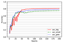
(b)

Figure 4: Linear model on noisy FashionMNIST, for $\lambda=0.01$.

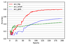
(a)

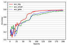
(b)

Figure 5: 2-layer neural network on noisy FashionMNIST, for $\lambda=0.01$.

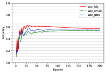
(a)

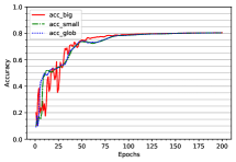
(b)

Figure 6: Linear model on noisy FashionMNIST, for $\lambda=0.1$.

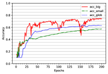
(a)

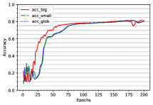
(b)

Figure 7: 2-layer neural network on noisy FashionMNIST, for $\lambda=0.1$.

(a)

(b)

Figure 8: Linear model on noisy FashionMNIST, for $\lambda=1$.

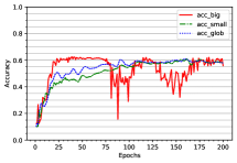
(a)

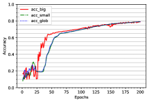
(b)

Figure 9: 2-layer neural network on noisy FashionMNIST, for $\lambda=1$.

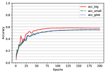
(a)

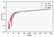
(b)

Figure 10: Linear model on noisy FashionMNIST, for $\lambda=10$.

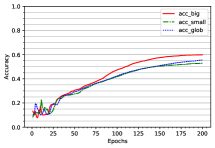
(a)

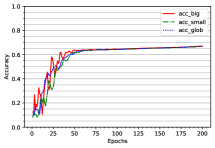
(b)

Figure 11: 2-layer neural network on noisy FashionMNIST, for $\lambda=10$.

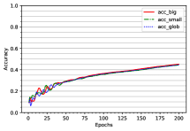
(a)

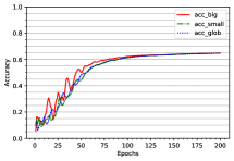
(b)

Figure 12: Linear model on noisy FashionMNIST, for $\lambda=100$.

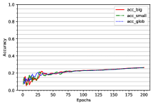
(a)

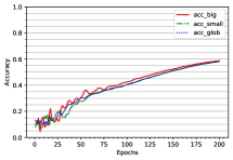
(b)

Figure 13: 2-layer neural network on noisy FashionMNIST, for $\lambda=100$.

E.2.2 FashionMNIST without noise

Recall that we introduced noise into FashionMNIST to make the problem harder to learn and observe a clear difference between the average and the sum. In this section, we present results of our experiments when the noise is removed.

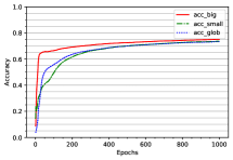
(a)

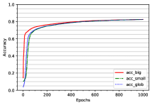
(b)

Figure 14: Linear model on FashionMNIST (without noise), for $\lambda=1$.

(a)

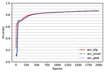
(b)

Figure 15: 2-layer neural network on FashionMNIST (without noise), for $\lambda=1$.

Even without noise, the difference between using the sum and using the expectation still seems important. We acknowledge, however, that the plots suggest that even though we ran this experiment for 10 times more (and 5 times more for the linear model) than other experiments, we might not have reached convergence yet, and that the use of the expectation might still eventually gets closer to the case of sum. We believe that the fact that the difference between sum and expectation in the absence of noise is weak is due to the fact that the FashionMNIST dataset is sufficiently linearly separable. Thus, we achieve a near-zero loss in both cases, which make the sum and the expectation close at optimum.

Even in this case, however, we observed that the sum clearly outperforms the expectation especially, in the first epochs. We argue that the reason for this is the following. By taking the average in local losses, the weights of the data of idle users are essentially blown out of proportion. As a result, the optimizer will very quickly fit these data. However, the signal from the data of the active user will then be too weak, so that the optimizer has to first almost perfectly fit the idle nodes’ data before it can catch the signal of the active user’s data and hence the average achieves weaker convergence performances than the sum.

Appendix F Linear Regression and Classification are Gradient PAC*

Throughout this section, we use the following terminology.

Definition 6.

Consider a parameterized event $\mathcal{E}(\mathcal{I})$. We say that the event $\mathcal{E}$ occurs with high probability if $\mathbb{P}\left[\mathcal{E}(\mathcal{I})\right]\rightarrow 1$ as $\mathcal{I}\rightarrow\infty$.

F.1 Preliminaries

Define $\left\lVert{\Sigma}\right\rVert_{2}\triangleq\max_{\left\lVert{x}\right\rVert_{2}\neq 0}(\left\lVert{\Sigma x}\right\rVert_{2}/\left\lVert{x}\right\rVert_{2})$ the $\ell_{2}$ operator norm of the matrix $\Sigma$. For symmetric matrices $\Sigma$, this is also the largest eigenvalue in absolute value.

Theorem 6 (Covariance concentration, Theorem 6.5 in (Wainwright, 2019)).

Denote $\Sigma=\mathbb{E}\left[\mathcal{Q}_{i}\mathcal{Q}_{i}^{T}\right]$, where $\mathcal{Q}_{i}\in\mathbb{R}^{d}$ is from a $\sigma_{\mathcal{Q}}$-sub-Gaussian random distribution $\tilde{\mathcal{Q}}$. Then, there are universal constants $c_{1}$, $c_{2}$ and $c_{3}$ such that, for any set $\left\{\mathcal{Q}_{i}\right\}_{i\in[\mathcal{I}]}$ of i.i.d. samples from $\tilde{\mathcal{Q}}$, and any $\delta>0$, the sample covariance $\widehat{\Sigma}=\frac{1}{\mathcal{I}}\sum\mathcal{Q}_{i}\mathcal{Q}_{i}^{T}$ satisfies the bound

$$\mathbb{P}\left[\frac{1}{\sigma_{\mathcal{Q}}^{2}}\left\lVert{\hat{\Sigma}-\Sigma}\right\rVert_{2}\geq c_{1}\left(\sqrt{\frac{d}{\mathcal{I}}}+\frac{d}{\mathcal{I}}\right)+\delta\right]\leq c_{2}\exp\left(-c_{3}\mathcal{I}\min(\delta,\delta^{2})\right).$$ (97)

Theorem 7 (Weyl’s Theorem, Theorem 4.3.1 in (Horn & Johnson, 2012)).

Let A and B be Hermitian and let the respective eigenvalues of $A$ and $B$ and $A+B$ be $\{\lambda_{i}(A)\}_{i=1}^{d}$, $\{\lambda_{i}(B)\}_{i=1}^{d}$, and $\{\lambda_{i}(A+B)\}_{i=1}^{d}$, each increasingly ordered. Then

$$\lambda_{i}(A+B)\leq\lambda_{i+j}(A)+\lambda_{d-j}(B),\quad j=0,1,...,d-i,$$ (98)

and

$$\lambda_{i+j}(A)+\lambda_{j+1}(B)\leq\lambda_{i}(A+B),\quad j=0,...,i-1,$$ (99)

for each $i=1,...,d$.

Lemma 20.

Consider two symmetric definite positive matrices $S$ and $\Sigma$. Denote $\rho_{min}$ and $\lambda_{min}$ their minimal eigenvalues. Then $\left\lvert{\rho_{min}-\lambda_{min}}\right\rvert\leq\left\lVert{S-\Sigma}\right\rVert_{2}$.

Proof.

This is a direct consequence of Theorem 7, for $A=S$, $B=\Sigma-S$, $i=1$, and $j=0$. ∎

Corollary 3.

There are universal constants $c_{1}$, $c_{2}$ and $c_{3}$ such that, for any $\sigma_{\mathcal{Q}}$-sub-Gaussian vector distribution $\tilde{\mathcal{Q}}\in\mathbb{R}^{d}$ and any $\delta>0$, the sample covariance $\widehat{\Sigma}=\frac{1}{\mathcal{I}}\sum\mathcal{Q}_{i}\mathcal{Q}_{i}^{T}$ satisfies the bound

$$\mathbb{P}\left[\frac{1}{\sigma_{\mathcal{Q}}^{2}}\left\lvert{\min\textsc{Sp}(\hat{\Sigma})-\min\textsc{Sp}(\Sigma)}\right\rvert\geq c_{1}\left(\sqrt{\frac{d}{\mathcal{I}}}+\frac{d}{\mathcal{I}}\right)+\delta\right]\leq c_{2}\exp\left(-c_{3}\mathcal{I}\min(\delta,\delta^{2})\right),$$ (100)

where $\min\textsc{Sp}(\hat{\Sigma})\text{ and }\min\textsc{Sp}(\Sigma)$ are the minimal eigenvalues of $\hat{\Sigma}$ and $\Sigma$.

Proof.

This follows from Theorem 6 and Lemma 20. ∎

Lemma 21.

With high probability, $\min\textsc{Sp}(\hat{\Sigma})\geq\min\textsc{Sp}(\Sigma)/2$.

Proof.

Denote $\lambda_{min}\triangleq\min\textsc{Sp}(\Sigma)$ and $\widehat{\lambda}_{min}\triangleq\min\textsc{Sp}(\hat{\Sigma})$. Since each $\mathcal{Q}_{i}$ is drawn i.i.d. from a $\sigma_{\mathcal{Q}}$-sub-Gaussian, we can apply Corollary 3. Namely, there are constants $c_{1}$, $c_{2}$ and $c_{3}$, such that for any $\delta>0$, we have

$$\mathbb{P}\left[\left\lvert{\widehat{\lambda}_{min}-\lambda_{min}}\right\rvert\geq c_{1}\sigma_{\mathcal{Q}}^{2}\left(\sqrt{\frac{d}{\mathcal{I}}}+\frac{d}{\mathcal{I}}\right)+\delta\sigma_{\mathcal{Q}}^{2}\right]\leq c_{2}\exp{(-c_{3}\mathcal{I}\min\left\{\delta,\delta^{2}\right\})}.$$ (101)

We now set $\delta\triangleq\lambda_{min}/(4\sigma_{\mathcal{Q}}^{2})$ and we consider $\mathcal{I}$ large enough so that $c_{1}\left(\sqrt{\frac{d}{\mathcal{I}}}+\frac{d}{\mathcal{I}}\right)\leq\lambda_{min}/(4\sigma_{\mathcal{Q}}^{2})$. With high probability, we then have $\widehat{\lambda}_{min}\geq\lambda_{min}/2$. ∎

F.2 Linear Regression is Gradient-PAC*

In this section, we prove the first part of Lemma 4. Namely, we prove that linear regression is gradient-PAC* learning.

F.2.1 Lemmas for linear regression

Before moving to the main proof that linear regression is gradient-PAC*, we first prove a few useful lemmas. These lemmas will rest on the following well-known theorems.

Theorem 8 (Lemma 2.7.7 in (Vershynin, 2018)).

If $X$ and $Y$ are sub-Gaussian, then $XY$ is sub-exponential.

Theorem 9 (Equation 2.18 in (Wainwright, 2019)).

If $X_{1},\ldots,X_{\mathcal{I}}$ are iid sub-exponential variables, then there exist constants $c_{4}$, $c_{5}$ such that, for all $\mathcal{I}$, we have

$$\forall t\in[0,c_{4}],~{}\mathbb{P}\left[\left\lvert{X-\mathbb{E}\left[X\right]}\right\rvert\geq t\mathcal{I}\right]\leq 2\exp\left(-c_{5}\mathcal{I}t^{2}\right).$$ (102)

Lemma 22.

For all $j\in[d]$, the random variables $X_{i}\triangleq\xi_{i}\mathcal{Q}_{i}[j]$ are iid, sub-exponential and have zero mean.

Proof.

The fact that these variables are iid follows straightforwardly from the fact that the noises $\xi_{i}$ are iid, and the queries $\mathcal{Q}_{i}$ are also iid. Moreover, both are sub-Gaussian, and by Theorem 8, the product of sub-Gaussian variables is sub-exponential. Finally, we have $\mathbb{E}\left[X\right]=\mathbb{E}\left[\xi\mathcal{Q}[j]\right]=\mathbb{E}\left[\xi\right]\mathbb{E}\left[\mathcal{Q}[j]\right]=0$, using the independence of the noise and the query, and the fact that noises have zero mean ($\mathbb{E}\left[\xi\right]=0$). ∎

Lemma 23.

There exists $B$ such that $\left\lVert{\sum_{i\in\mathcal{I}}\xi_{i}\mathcal{Q}_{i}}\right\rVert_{2}\leq B\mathcal{I}^{3/4}$ with high probability.

Proof.

By Lemma 22, the terms $\xi_{i}\mathcal{Q}_{i}[j]$ are iid, sub-exponential and have zero mean. Therefore, by Theorem 9, there exist constants $c_{4}$ and $c_{5}$ such that for any coordinate $j\in[d]$ of $\xi_{i}\mathcal{Q}_{i}$ and for all $0\leq u\leq c_{4}$, we have

$$\mathbb{P}\left[\left\lvert{\sum_{i\in\mathcal{I}}\xi_{i}\mathcal{Q}_{i}[j]}\right\rvert\geq\mathcal{I}u\right]\leq 2\exp{(-c_{5}\mathcal{I}u^{2})}.$$ (103)

Plugging $u=v\mathcal{I}^{(-1/4)}$ into the inequality for some small enough constant $v$, and using union bound then yields

$$\mathbb{P}\left[\left\lVert{\sum_{i\in\mathcal{I}}\xi_{i}\mathcal{Q}_{i}}\right\rVert_{2}\geq\mathcal{I}^{(3/4)}v\sqrt{d}\right]\leq\mathbb{P}\left[\left\lVert{\sum_{i\in\mathcal{I}}\xi_{i}\mathcal{Q}_{i}}\right\rVert_{\infty}\geq\mathcal{I}^{(3/4)}v\right]\leq 2d\exp{(-c_{5}\sqrt{\mathcal{I}}v^{2})}.$$ (104)

Defining $B\triangleq v\sqrt{d}$ yields the lemma. ∎

F.2.2 Proof that linear regression is gradient-PAC*

We now move on to proving that least square linear regression is gradient-PAC*.

Proof of Theorem 2.

Note that $\nabla_{\theta}\ell(\theta,\mathcal{Q},\mathcal{A})=(\theta^{T}\mathcal{Q}-\mathcal{A})\mathcal{Q}$. Thus, on input $i\in[\mathcal{I}]$, we have

$$\nabla_{\theta}\ell(\theta,\mathcal{Q}_{i},\mathcal{A}(\mathcal{Q}_{i},\theta^{\dagger}))=\left((\theta-\theta^{\dagger})^{T}\mathcal{Q}_{i}\right)\mathcal{Q}_{i}-\xi_{i}\mathcal{Q}_{i}.$$ (105)

Moreover, we have

$$(\theta-\theta^{\dagger})^{T}\nabla_{\theta}\left(\nu\left\lVert{\theta}\right\rVert_{2}^{2}\right)=2\nu(\theta-\theta^{\dagger})^{T}\theta=2\nu\left\lVert{\theta-\theta^{\dagger}}\right\rVert_{2}^{2}+2\nu(\theta-\theta^{\dagger})^{T}\theta^{\dagger}.$$ (106)

As a result, we have

$$(\theta-\theta^{\dagger})^{T}\nabla_{\theta}\mathcal{L}(\theta,\mathcal{D})=$$ (107)

$$\mathcal{I}(\theta-\theta^{\dagger})^{T}\widehat{\Sigma}(\theta-\theta^{\dagger})-(\theta-\theta^{\dagger})^{T}\left(\sum_{i\in\mathcal{I}}\xi_{i}\mathcal{Q}_{i}\right)+2\nu\left\lVert{\theta-\theta^{\dagger}}\right\rVert_{2}^{2}+2\nu(\theta-\theta^{\dagger})^{T}\theta^{\dagger}.$$ (108)

But now, with high probability, we have $(\theta-\theta^{\dagger})^{T}\widehat{\Sigma}(\theta-\theta^{\dagger})\geq(\lambda_{min}/2)\left\lVert{\theta-\theta^{\dagger}}\right\rVert_{2}^{2}$ (Lemma 21) and $\left\lVert{\sum_{i\in\mathcal{I}}\xi_{i}\mathcal{Q}_{i}}\right\rVert_{2}\leq B\mathcal{I}^{(3/4)}$ (Lemma 23). Using the fact that $\left\lVert{\theta^{\dagger}}\right\rVert_{2}\leq\mathcal{K}$ and the Cauchy-Schwarz inequality, we have

$$(\theta-\theta^{\dagger})^{T}\nabla_{\theta}\mathcal{L}(\theta,\mathcal{D}) \geq(\frac{\lambda_{min}}{2}\mathcal{I}+\nu)\left\lVert{\theta-\theta^{\dagger}}\right\rVert_{2}^{2}-(B\mathcal{I}^{(3/4)}+2\nu\mathcal{K})\left\lVert{\theta-\theta^{\dagger}}\right\rVert_{2}.$$ (109)

Denoting $A_{\mathcal{K}}\triangleq\frac{\lambda_{min}}{2}$ and $B_{\mathcal{K}}\triangleq B+2\nu\mathcal{K}$ and using the fact that $\mathcal{I}\geq 1$, we then have

$$(\theta-\theta^{\dagger})^{T}\nabla_{\theta}\mathcal{L}(\theta,\mathcal{D}) \geq A_{\mathcal{K}}\mathcal{I}\left\lVert{\theta-\theta^{\dagger}}\right\rVert_{2}^{2}-B_{\mathcal{K}}\mathcal{I}^{(3/4)}\left\lVert{\theta-\theta^{\dagger}}\right\rVert_{2}$$ (110)

$$\geq A_{\mathcal{K}}\mathcal{I}\min\left\{\left\lVert{\theta-\theta^{\dagger}}\right\rVert_{2},\left\lVert{\theta-\theta^{\dagger}}\right\rVert_{2}^{2}\right\}-B_{\mathcal{K}}\mathcal{I}^{(3/4)}\left\lVert{\theta-\theta^{\dagger}}\right\rVert_{2},$$ (111)

with high probability. This corresponds to saying Assumption 3 is satisfied for $\alpha=3/4$. ∎

F.3 Logistic Regression

In this section, we now prove the second part of Lemma 4. Namely, we prove that logistic regression is gradient-PAC* learning.

F.3.1 Lemmas about the sigmoid function

We first prove two useful lemmas about the following logistic distance function.

Definition 7.

We define the logistic distance function by $\Delta(a,b)\triangleq(a-b)\left(\sigma(a)-\sigma(b)\right)$.

Lemma 24.

If $a,b\in\mathbb{R}$ such that for some $k>0$, $\left\lvert{a}\right\rvert\leq k$ and $\left\lvert{b}\right\rvert\leq k$, then there exists some constant $c_{k}>0$ such that

$$\Delta(a,b)\geq c_{k}\left\lvert{a-b}\right\rvert^{2}.$$ (112)

Proof.

Note that the derivative of $\sigma(z)$ is strictly positive, symmetric ($\sigma^{\prime}(z)=\sigma^{\prime}(-z)$) and monotonically decreasing for $z\geq 0$. Therefore, for any $z\in[-k,k]$, we know $\sigma^{\prime}(z)\geq c_{k}\triangleq\sigma^{\prime}(k)$. Thus, by the mean value theorem, we have

$$\frac{\sigma(a)-\sigma(b)}{a-b}\geq c_{k}.$$ (113)

Multiplying both sides by $(a-b)^{2}$ then yields the lemma. ∎

Lemma 25.

If $b\in\mathbb{R}$, and $\left\lvert{b}\right\rvert\leq k$, for some $k>0$, then there exists a constant $d_{k}$, such that for any $a\in\mathbb{R}$, we have

$$\Delta(a,b)\geq d_{k}\left\lvert{a-b}\right\rvert-d_{k}$$ (114)

Proof.

Assume $\left\lvert{a-b}\right\rvert\geq 1$ and define $d_{k}\triangleq\sigma(k+1)-\sigma(k)$. If $b\geq 0$, since $\sigma^{\prime}(z)$ is decreasing for $z\geq 0$, we have $\sigma(b)-\sigma(b-1)\geq\sigma(b+1)-\sigma(b)\geq d_{k}$, and by symmetry, a similar argument holds for $b\leq 0$. Thus, we have

$$\left\lvert{\sigma(a)-\sigma(b)}\right\rvert\geq\min\left\{\sigma(b)-\sigma(b-1),\sigma(b+1)-\sigma(b)\right\}\geq d_{k}.$$ (115)

Therefore,

$$(a-b)\left(\sigma(a)-\sigma(b)\right)\geq d_{k}\left\lvert{a-b}\right\rvert\geq d_{k}\left\lvert{a-b}\right\rvert-d_{k}.$$ (116)

For the case of $\left\lvert{a-b}\right\rvert\leq 1$, we also have $(a-b)\left(\sigma(a)-\sigma(b)\right)\geq 0\geq d_{k}\left\lvert{a-b}\right\rvert-d_{k}$. ∎

F.3.2 A uniform lower bound

Definition 8.

Denote $\mathbb{S}^{d-1}\triangleq\left\{{\bf u}\in\mathbb{R}^{d}\,\middle|\,\left\lVert{{\bf u}}\right\rVert_{2}=1\right\}$ the hypersphere in $\mathbb{R}^{d}$.

Lemma 26.

Assume $\textsc{Supp}(\tilde{\mathcal{Q}})$ spans $\mathbb{R}^{d}$. Then, for all ${\bf u}\in\mathbb{S}^{d-1}$, $\mathbb{E}\left[\left\lvert{\mathcal{Q}^{T}{\bf u}}\right\rvert\right]>0$.

Proof.

Let ${\bf u}\in\mathbb{S}^{d-1}$. We know that there exists $\mathcal{Q}_{1},\ldots,\mathcal{Q}_{d}\in\textsc{Supp}(\tilde{\mathcal{Q}})$ and $\alpha_{1},\ldots,\alpha_{d}\in\mathbb{R}$ such that ${\bf u}$ is colinear with $\sum\alpha_{j}\mathcal{Q}_{j}$. In particular, we then have ${\bf u}^{T}\sum\alpha_{j}\mathcal{Q}_{j}=\sum\alpha_{j}(\mathcal{Q}_{j}^{T}{\bf u})\neq 0$. Therefore, there must be a query $\mathcal{Q}_{*}\in\textsc{Supp}(\tilde{\mathcal{Q}})$ such that $\mathcal{Q}_{*}^{T}{\bf u}\neq 0$, which implies $a\triangleq\left\lvert{\mathcal{Q}_{*}^{T}{\bf u}}\right\rvert>0$ By continuity of the scalar product, there must then also exist $\varepsilon>0$ such that, for any $\mathcal{Q}\in\mathcal{B}(\mathcal{Q}_{*},\varepsilon)$, we have $\left\lvert{\mathcal{Q}^{T}{\bf u}}\right\rvert\geq a/2$, where $\mathcal{B}(\mathcal{Q}_{*},\varepsilon)$ is an Euclidean ball centered on $\mathcal{Q}_{*}$ and of radius $\varepsilon$.

But now, by definition of the support, we know that $p\triangleq\mathbb{P}\left[\mathcal{Q}\in\mathcal{B}(\mathcal{Q}_{*},\varepsilon)\right]>0$. By the law of total expectation, we then have

$$\mathbb{E}\left[\left\lvert{\mathcal{Q}^{T}{\bf u}}\right\rvert\right] =\mathbb{E}\left[\left\lvert{\mathcal{Q}^{T}{\bf u}}\right\rvert\,\middle|\,\mathcal{Q}\in\mathcal{B}(\mathcal{Q}_{*},\varepsilon)\right]\mathbb{P}\left[\mathcal{Q}\in\mathcal{B}(\mathcal{Q}_{*},\varepsilon)\right]$$

$$\qquad\qquad+\mathbb{E}\left[\left\lvert{\mathcal{Q}^{T}{\bf u}}\right\rvert\,\middle|\,\mathcal{Q}\notin\mathcal{B}(\mathcal{Q}_{*},\varepsilon)\right]\mathbb{P}\left[\mathcal{Q}\notin\mathcal{B}(\mathcal{Q}_{*},\varepsilon)\right]$$ (117)

$$\geq ap/2+0>0,$$ (118)

which is the lemma. ∎

Lemma 27.

Assume that, for all unit vectors ${\bf u}\in\mathbb{S}^{d-1}$, we have $\mathbb{E}\left[\left\lvert{\mathcal{Q}^{T}{\bf u}}\right\rvert\right]>0$, and that $\textsc{Supp}(\tilde{\mathcal{Q}})$ is bounded by $M_{\mathcal{Q}}$. Then there exists $C>0$ such that, with high probability,

$$\forall{\bf u}\in\mathbb{S}^{d-1},~{}\sum_{i\in\mathcal{I}}\left\lvert{\mathcal{Q}_{i}^{T}{\bf u}}\right\rvert\geq C\mathcal{I}.$$ (119)

Proof.

By continuity of the scalar product and the expectation operator, and by compactness of $\mathbb{S}^{d-1}$, we know that

$$C_{0}\triangleq\inf_{{\bf u}\in\mathbb{R}^{d}}\mathbb{E}\left[\left\lvert{\mathcal{Q}^{T}{\bf u}}\right\rvert\right]>0.$$ (120)

Now define $\varepsilon\triangleq C_{0}/4M_{\mathcal{Q}}$. Note that $\mathbb{S}^{d-1}\subset\bigcup_{{\bf u}\in\mathbb{S}^{d-1}}\mathcal{B}({\bf u},\varepsilon)$. Thus we have a covering of the hypersphere by open sets. But since $\mathbb{S}^{d-1}$ is compact, we know that we can extract a finite covering. In other words, there exists a finite subset $S\subset\mathbb{S}^{d-1}$ such that $\mathbb{S}^{d-1}\subset\bigcup_{{\bf u}\in S}\mathcal{B}({\bf u},\varepsilon)$. Put differently, for any ${\bf v}\in\mathbb{S}^{d-1}$, there exists ${\bf u}\in S$ such that $\left\lVert{{\bf u}-{\bf v}}\right\rVert_{2}\leq\varepsilon$.

Now consider ${\bf u}\in S$. Given that $\textsc{Supp}(\tilde{\mathcal{Q}})$ is bounded, we know that $\left\lvert{\mathcal{Q}_{i}^{T}{\bf u}}\right\rvert\in[0,M_{\mathcal{Q}}]$. Moreover, such variables $\left\lvert{\mathcal{Q}_{i}^{T}{\bf u}}\right\rvert$ are iid. By Hoeffding’s inequality, for any $t>0$, we have

$$\mathbb{P}\left[\left\lvert{\sum_{i\in\mathcal{I}}\left\lvert{\mathcal{Q}_{i}^{T}{\bf u}}\right\rvert-\mathcal{I}\mathbb{E}\left[\left\lvert{\mathcal{Q}^{T}\ {\bf u}}\right\rvert\right]}\right\rvert\geq\mathcal{I}t\right]\leq 2\exp\left(\frac{-2\mathcal{I}t^{2}}{M_{\mathcal{Q}}}\right).$$ (121)

Choosing $t=C_{0}/2$ then yields

$$\mathbb{P}\left[\sum_{i\in\mathcal{I}}\left\lvert{\mathcal{Q}_{i}^{T}{\bf u}}\right\rvert\leq\frac{C_{0}\mathcal{I}}{2}\right] \leq\mathbb{P}\left[\left\lvert{\sum_{i\in\mathcal{I}}\left\lvert{\mathcal{Q}_{i}^{T}{\bf u}_{\theta-\theta^{\dagger}}}\right\rvert-\mathcal{I}\mathbb{E}\left[\left\lvert{\mathcal{Q}^{T}\ {\bf u}_{\theta-\theta^{\dagger}}}\right\rvert\right]}\right\rvert\geq\frac{\mathcal{I}C_{0}}{2}\right]$$ (122)

$$\leq 2\exp\left(\frac{-\mathcal{I}{C_{0}}^{2}}{2M_{\mathcal{Q}}}\right).$$ (123)

Taking a union bound for ${\bf u}\in S$ then guarantees

$$\mathbb{P}\left[\forall{\bf u}\in S,~{}\sum_{i\in\mathcal{I}}\left\lvert{\mathcal{Q}_{i}^{T}{\bf u}}\right\rvert\geq\frac{C_{0}\mathcal{I}}{2}\right]\geq 1-2\left\lvert{S}\right\rvert\exp\left(\frac{-\mathcal{I}{C_{0}}^{2}}{2M_{\mathcal{Q}}}\right),$$ (124)

which clearly goes to 1 as $\mathcal{I}\rightarrow\infty$. Thus $\forall{\bf u}\in S,~{}\sum_{i\in\mathcal{I}}\left\lvert{\mathcal{Q}_{i}^{T}{\bf u}}\right\rvert\geq\frac{C_{0}\mathcal{I}}{2}$ holds with high probability.

Now consider ${\bf v}\in\mathbb{S}^{d-1}$. We know that there exists ${\bf u}\in S$ such that $\left\lVert{{\bf u}-{\bf v}}\right\rVert_{2}\leq\varepsilon$. Then, we have

$$\sum_{i\in[\mathcal{I}]}\left\lvert{\mathcal{Q}_{i}^{T}{\bf v}}\right\rvert =\sum_{i\in[\mathcal{I}]}\left\lvert{\mathcal{Q}_{i}^{T}{\bf u}+\mathcal{Q}_{i}^{T}({\bf v}-{\bf u})}\right\rvert$$ (125)

$$\geq\sum_{i\in[\mathcal{I}]}\left\lvert{\mathcal{Q}_{i}^{T}{\bf u}}\right\rvert-\mathcal{I}M_{\mathcal{Q}}\left\lVert{{\bf v}-{\bf u}}\right\rVert_{2}$$ (126)

$$\geq\frac{C_{0}\mathcal{I}}{2}-\mathcal{I}M_{\mathcal{Q}}\frac{C_{0}}{4M_{\mathcal{Q}}}=\frac{C_{0}\mathcal{I}}{4},$$ (127)

which proves the lemma. ∎

F.3.3 Lower bound on the discrepancy between preferred and reported answers

Lemma 28.

Assume that $\tilde{\mathcal{Q}}$ has a bounded support, whose interior contains the origin. Suppose also that $\left\lVert{\theta^{\dagger}}\right\rVert_{2}\leq\mathcal{K}$. Then there exists $A_{\mathcal{K}}$ such that, with high probability, we have

$$\sum_{i\in[\mathcal{I}]}\Delta(\mathcal{Q}_{i{}}^{T}\theta,\mathcal{Q}_{i{}}^{T}\theta^{\dagger})\geq A_{\mathcal{K}}\mathcal{I}\min\left\{\left\lVert{\theta-\theta^{\dagger}}\right\rVert_{2},\left\lVert{\theta-\theta^{\dagger}}\right\rVert_{2}^{2}\right\}.$$ (128)

Proof.

Note that by Cauchy-Schwarz inequality we have

$$\left\lvert{\mathcal{Q}_{i}^{T}\theta^{\dagger}}\right\rvert\leq\left\lVert{\mathcal{Q}_{i}}\right\rVert_{2}\left\lVert{\theta^{\dagger}}\right\rVert_{2}\leq M_{\mathcal{Q}}\mathcal{K}.$$ (129)

Thus, Lemma 25 implies the existence of a positive constant $d_{\mathcal{K}}$, such that for all $\theta\in\mathbb{R}^{d}$, we have

$$\sum_{i\in\mathcal{I}}\Delta\left(\mathcal{Q}_{i}^{T}\theta,\mathcal{Q}_{i}^{T}\theta^{\dagger}\right) \geq\sum_{i\in\mathcal{I}}\left(d_{\mathcal{K}}\left\lvert{\mathcal{Q}_{i}^{T}\theta-\mathcal{Q}_{i}^{T}\theta^{\dagger}}\right\rvert-d_{\mathcal{K}}\right)$$ (130)

$$=-d_{\mathcal{K}}\mathcal{I}+d_{\mathcal{K}}\left\lVert{\theta-\theta^{\dagger}}\right\rVert_{2}\sum_{i\in\mathcal{I}}\left\lvert{\mathcal{Q}_{i}^{T}{\bf u}_{\theta-\theta^{\dagger}}}\right\rvert,$$ (131)

where ${\bf u}_{\theta-\theta^{\dagger}}\triangleq(\theta-\theta^{\dagger})/\left\lVert{\theta-\theta^{\dagger}}\right\rVert_{2}$ is the unit vector in the direction of $\theta-\theta^{\dagger}$.

Now, by Lemma 27, we know that, with high probability, for all unit vectors ${\bf u}\in\mathbb{S}^{d-1}$, we have $\sum\left\lvert{\mathcal{Q}_{i}^{T}{\bf u}}\right\rvert\geq C\mathcal{I}$. Thus, for $\mathcal{I}$ sufficiently large, for any $\theta\in\mathbb{R}^{d}$, with high probability, we have

$$\sum_{i\in\mathcal{I}}\Delta(\mathcal{Q}_{i{}}^{T}\theta,\mathcal{Q}_{i{}}^{T}\theta^{\dagger})\geq\frac{d_{\mathcal{K}}C_{min}}{2}\mathcal{I}\left\lVert{\theta-\theta^{\dagger}}\right\rVert_{2}-d_{\mathcal{K}}\mathcal{I}.$$ (132)

Defining $e_{\mathcal{K}}\triangleq\frac{d_{\mathcal{K}}C_{min}}{4}$, and $f_{\mathcal{K}}\triangleq\frac{4}{C_{min}}$, for $\left\lVert{\theta-\theta^{\dagger}}\right\rVert_{2}>f_{\mathcal{K}}$, we then have

$$\sum_{i\in\mathcal{I}}\Delta(\mathcal{Q}_{i{}}^{T}\theta,\mathcal{Q}_{i{}}^{T}\theta^{\dagger})\geq e_{\mathcal{K}}\mathcal{I}\left\lVert{\theta-\theta^{\dagger}}\right\rVert_{2}.$$ (133)

We now focus on the case of $\left\lVert{\theta-\theta^{\dagger}}\right\rVert_{2}\leq f_{\mathcal{K}}$. The triangle inequality yields $\left\lVert{\theta}\right\rVert_{2}\leq\left\lVert{\theta-\theta^{\dagger}}\right\rVert_{2}+\left\lVert{\theta^{\dagger}}\right\rVert_{2}\leq f_{\mathcal{K}}+\mathcal{K}$. By Cauchy-Schwarz inequality, we then have $\left\lvert{\mathcal{Q}_{i}^{T}\theta}\right\rvert\leq(f_{\mathcal{K}}+\mathcal{K})M_{\mathcal{Q}}\triangleq g_{\mathcal{K}}$ and $\left\lvert{\mathcal{Q}_{i}^{T}\theta^{\dagger}}\right\rvert\leq\mathcal{K}M_{\mathcal{Q}}\leq g_{\mathcal{K}}$. Thus, by Lemma 24, we know there exists some constant $c_{\mathcal{K}}$ such that

$$\sum_{i\in\mathcal{I}}\left(\sigma(\mathcal{Q}_{i}^{T}\theta)-\sigma(\mathcal{Q}_{i}^{T}\theta^{\dagger})\right)(\mathcal{Q}_{i}^{T}\theta-\mathcal{Q}_{i}^{T}\theta^{\dagger}) \geq\sum_{i\in\mathcal{I}}c_{\mathcal{K}}\left\lvert{\mathcal{Q}_{i}^{T}\theta-\mathcal{Q}_{i}^{T}\theta^{\dagger}}\right\rvert^{2}$$ (134)

$$=\sum_{i\in\mathcal{I}}c_{\mathcal{K}}(\theta-\theta^{\dagger})^{T}\mathcal{Q}_{i}\mathcal{Q}_{i}^{T}(\theta-\theta^{\dagger})$$ (135)

$$=c_{\mathcal{K}}(\theta-\theta^{\dagger})^{T}\left(\sum_{i\in\mathcal{I}}\mathcal{Q}_{i}\mathcal{Q}_{i}^{T}\right)(\theta-\theta^{\dagger}).$$ (136)

Since distribution $\tilde{\mathcal{Q}}$ is bounded (and thus sub-Gaussian), by Theorem 6, with high probability, we have

$$(\theta-\theta^{\dagger})^{T}\left(\sum_{i\in\mathcal{I}}\mathcal{Q}_{i}\mathcal{Q}_{i}^{T}\right)(\theta-\theta^{\dagger})\geq\frac{\lambda_{min}}{2}\mathcal{I}\left\lVert{\theta-\theta^{\dagger}}\right\rVert_{2}^{2},$$ (137)

where $\lambda_{min}$ is the smallest eigenvalue of $\mathbb{E}\left[\mathcal{Q}_{i}\mathcal{Q}_{i}^{T}\right]$. Thus, for $\left\lVert{\theta-\theta^{\dagger}}\right\rVert_{2}\leq f_{\mathcal{K}}$, we have

$$\sum_{i\in\mathcal{I}}\left(\sigma(\mathcal{Q}_{i}^{T}\theta)-\sigma(\mathcal{Q}_{i}^{T}\theta^{\dagger})\right)(\mathcal{Q}_{i}^{T}\theta-\mathcal{Q}_{i}^{T}\theta^{\dagger})\geq\frac{\lambda_{min}c_{\mathcal{K}}}{2}\mathcal{I}\left\lVert{\theta-\theta^{\dagger}}\right\rVert_{2}^{2}.$$ (138)

Combining this with (133), and defining $A_{\mathcal{K}}\triangleq\min\left\{\frac{\lambda_{min}c_{\mathcal{K}}}{2},e_{\mathcal{K}}\right\}$, we then obtain the lemma. ∎

F.3.4 Proof that logistic regression is gradient-PAC*

Now we proceed with the proof that logistic regression is gradient-PAC*.

Proof of Theorem 3.

Note that $\sigma(-z)=e^{-z}\sigma(z)=1-\sigma(z)$ and $\sigma^{\prime}(z)=e^{-z}\sigma^{2}(z)$. We then have

$$\nabla_{\theta}\ell(\theta,\mathcal{Q},\mathcal{A}) =-\frac{\sigma^{\prime}(\mathcal{A}\mathcal{Q}^{T}\theta)\mathcal{A}\mathcal{Q}}{\sigma(\mathcal{A}\mathcal{Q}^{T}\theta)}=-e^{-\mathcal{A}\mathcal{Q}^{T}\theta}\sigma(\mathcal{A}\mathcal{Q}^{T}\theta)\mathcal{A}\mathcal{Q}$$ (139)

$$=-\sigma(-\mathcal{A}\mathcal{Q}^{T}\theta)\mathcal{A}\mathcal{Q}=\left(\sigma(\mathcal{Q}^{T}\theta)-\mathbbm{1}\left[\mathcal{A}=1\right]\right)\mathcal{Q},$$ (140)

where $\mathbbm{1}\left[\mathcal{A}=1\right]$ is the indicator function that outputs $1$ if $\mathcal{A}=1$, and $0$ otherwise. As a result,

$$(\theta-\theta^{\dagger})^{T}\nabla_{\theta}\mathcal{L}(\theta,\mathcal{D})=$$ (141)

$$(\theta-\theta^{\dagger})^{T}\left(\sum_{i\in\mathcal{I}}\left(\sigma(\mathcal{Q}_{i}^{T}\theta)-\mathbbm{1}\left[\mathcal{A}_{i}=1\right]\right)\mathcal{Q}_{i}\right)+2\nu(\theta-\theta^{\dagger})^{T}\theta$$ (142)

$$=(\theta-\theta^{\dagger})^{T}\left(\sum_{i\in\mathcal{I}}\left(\sigma(\mathcal{Q}_{i}^{T}\theta)-\sigma(\mathcal{Q}_{i}^{T}\theta^{\dagger})+\sigma(\mathcal{Q}_{i}^{T}\theta^{\dagger})-\mathbbm{1}\left[\mathcal{A}_{i}=1\right]\right)\mathcal{Q}_{i}\right)$$ (143)

$$+2\nu\left\lVert{\theta-\theta^{\dagger}}\right\rVert_{2}^{2}+2\nu(\theta-\theta^{\dagger})^{T}\theta^{\dagger}$$ (144)

$$=\sum_{i\in[\mathcal{I}]}\Delta\left(\mathcal{Q}_{i}^{T}\theta,\mathcal{Q}_{i}^{T}\theta^{\dagger}\right)+(\theta-\theta^{\dagger})^{T}\left(\sum_{i\in\mathcal{I}}\left(\sigma(\mathcal{Q}_{i}^{T}\theta^{\dagger})-\mathbbm{1}\left[\mathcal{A}_{i}=1\right]\right)\mathcal{Q}_{i}\right)$$ (145)

$$+2\nu\left\lVert{\theta-\theta^{\dagger}}\right\rVert_{2}^{2}+2\nu(\theta-\theta^{\dagger})^{T}\theta^{\dagger}.$$ (146)

By Lemma 28, with high probability, we have

$$\sum_{i\in[\mathcal{I}]}\Delta\left(\mathcal{Q}_{i}^{T}\theta,\mathcal{Q}_{i}^{T}\theta^{\dagger}\right)\geq A_{\mathcal{K}}\mathcal{I}\min\left\{\left\lVert{\theta-\theta^{\dagger}}\right\rVert_{2},\left\lVert{\theta-\theta^{\dagger}}\right\rVert_{2}^{2}\right\}.$$ (147)

To control the second term of (145), note that the random vectors $Z_{i}\triangleq\left(\sigma(\mathcal{Q}_{i}^{T}\theta^{\dagger})-\mathbbm{1}\left[\mathcal{A}_{i}=1\right]\right)\mathcal{Q}_{i}$ are iid with norm at most $M_{\mathcal{Q}}$. Moreover, since $\mathbb{E}\left[\mathbbm{1}\left[\mathcal{A}_{i}=1\right]|\mathcal{Q}_{i}\right]=\sigma(\mathcal{Q}_{i}^{T}\theta^{\dagger})$, by the tower rule, we have $\mathbb{E}\left[Z_{i}\right]=\mathbb{E}\left[\mathbb{E}\left[Z_{i}|\mathcal{Q}_{i}\right]\right]=0$. Therefore, by applying Hoeffding’s bound to every coordinate of $Z_{i}$, and then taking a union bound, for any $B>0$, we have

$$\mathbb{P}\left[\left\lVert{\sum_{i\in\mathcal{I}}Z_{i}}\right\rVert_{2}\geq B\mathcal{I}^{3/4}\right]\leq 2d\exp\left(-\frac{B^{2}\sqrt{\mathcal{I}}}{2dM_{\mathcal{Q}}^{2}}\right).$$ (148)

Applying now Cauchy-Schwarz inequality, with high probability, we have

$$\left\lvert{(\theta-\theta^{\dagger})^{T}\left(\sum_{i\in\mathcal{I}}\left(\sigma(\mathcal{Q}_{i}^{T}\theta^{\dagger})-\mathbbm{1}\left[\mathcal{A}_{i}=1\right]\right)\mathcal{Q}_{i}\right)}\right\rvert\leq B\mathcal{I}^{3/4}\left\lVert{\theta-\theta^{\dagger}}\right\rVert_{2}.$$

Combining this with (138) and using $\left\lVert{\theta^{\dagger}}\right\rVert_{2}^{2}\leq\mathcal{K}$, we then have

$$(\theta-\theta^{\dagger})^{T}\nabla_{\theta}\mathcal{L}(\theta,\mathcal{D})$$ (149)

$$\geq(A_{\mathcal{K}}\mathcal{I}+\nu)\left\{\left\lVert{\theta-\theta^{\dagger}}\right\rVert_{2},\left\lVert{\theta-\theta^{\dagger}}\right\rVert_{2}^{2}\right\}-(B\mathcal{I}^{(3/4)}+2\nu\mathcal{K})\left\lVert{\theta-\theta^{\dagger}}\right\rVert_{2}$$ (150)

$$\geq A_{\mathcal{K}}\mathcal{I}\left\{\left\lVert{\theta-\theta^{\dagger}}\right\rVert_{2},\left\lVert{\theta-\theta^{\dagger}}\right\rVert_{2}^{2}\right\}-B_{\mathcal{K}}\mathcal{I}^{(3/4)}\left\lVert{\theta-\theta^{\dagger}}\right\rVert_{2},$$ (151)

where $B_{\mathcal{K}}=B+2\nu\mathcal{K}$. This shows that Assumption 3 is satisfied for logistic loss for $\alpha=3/4$, and $A_{\mathcal{K}}$ and $B_{\mathcal{K}}$ as previously defined.

∎

Appendix G Proofs of Local PAC*-Learnability

Let us now prove Lemma 5. To do so, consider the preferred models $\vec{\theta}^{\dagger}$ and a subset $\mathcal{H}\subset[N]$ of honest users. Denote $\vec{\mathcal{D}}_{-\mathcal{H}}$ the datasets provided by users $n\in[N]-\mathcal{H}$. Each honest user $h\in\mathcal{H}$ provides an honest dataset $\mathcal{D}_{h}$ of cardinality at least $\mathcal{I}\geq 1$. Consider the bound $K_{\mathcal{H}}\triangleq\max_{h\in\mathcal{H}}\left\lVert{\theta_{h}^{\dagger}}\right\rVert_{2}$ on the parameter norm of honest active users $h\in\mathcal{H}$.

G.1 Bounds on the Optima

Before proving the theorem, we prove a useful lemma that bounds the set of possible values for the global model and honest local models.

Lemma 29.

Assume that $\mathcal{R}$ and $\ell$ are nonnegative. For $\mathcal{I}$ large enough, if all honest active users $h\in\mathcal{H}$ provide at least $\mathcal{I}$ data, then, with high probability, $\vec{\theta}^{*}_{\mathcal{H}}$ must lie in a compact subset of $\mathbb{R}^{d\times\mathcal{H}}$ that does not depend on $\mathcal{I}$.

Proof.

Denote $L^{0}\triangleq\textsc{Loss}{}(0,(\vec{\theta}^{\dagger}_{H},0_{-\mathcal{H}}),(\emptyset,\vec{\mathcal{D}}_{-\mathcal{H}}))$. Essentially, we will show that, if $\vec{\theta}^{*}_{\mathcal{H}}$ is too far from $\vec{\theta}^{\dagger}_{\mathcal{H}}$, then the loss will take values strictly larger than $L^{0}$.

Assumption 3 implies the existence of an event $\mathcal{E}$ that occurs with probability at least $P_{0}\triangleq P(K_{\mathcal{H}},\mathcal{I})^{\left\lvert{\mathcal{H}}\right\rvert}$, under which, for any $\theta_{h}\in\mathbb{R}^{d}$, we have

$$\left(\theta_{h}-\theta_{h}^{\dagger}\right)^{T}\nabla\mathcal{L}_{h}\left(\theta_{h}\right)\geq A_{K_{\mathcal{H}}}\mathcal{I}\min\left\{\left\lVert{\theta_{h}-\theta_{h}^{\dagger}}\right\rVert_{2},\left\lVert{\theta_{h}-\theta_{h}^{\dagger}}\right\rVert_{2}^{2}\right\}-B_{K_{\mathcal{H}}}\mathcal{I}^{\alpha}\left\lVert{\theta_{h}-\theta_{h}^{\dagger}}\right\rVert_{2},$$ (152)

which implies

$${\bf u}_{\left(\theta_{h}-\theta_{h}^{\dagger}\right)}^{T}\nabla\mathcal{L}_{h}\left(\theta_{h}\right)\geq A_{K_{\mathcal{H}}}\mathcal{I}\min\left\{1,\left\lVert{\theta_{h}-\theta_{h}^{\dagger}}\right\rVert_{2}\right\}-B_{K_{\mathcal{H}}}\mathcal{I}^{\alpha}.$$ (153)

Note also that $P_{0}\rightarrow 1$ as $\mathcal{I}\rightarrow\infty$. We now integrate both sides over the line segment from $\theta_{h}^{\dagger}$ to $\theta_{h}$. The fundamental theorem of calculus for line integrals then yields

$$\mathcal{L}_{h}\left(\theta_{h}\right)-\mathcal{L}_{h}\left(\theta_{h}^{\dagger}\right)=\left\lVert{\theta_{h}-\theta_{h}^{\dagger}}\right\rVert_{2}\int_{t=0}^{1}{\bf u}_{\left(\theta_{h}-\theta_{h}^{\dagger}\right)}^{T}\nabla\mathcal{L}\left(\theta_{h}^{\dagger}+t(\theta_{h}-\theta_{h}^{\dagger})\right)dt$$ (154)

$$\geq\left\lVert{\theta_{h}-\theta_{h}^{\dagger}}\right\rVert_{2}\int_{t=0}^{1}\left(A_{K_{\mathcal{H}}}\mathcal{I}\min\left\{1,t\left\lVert{\theta_{h}-\theta_{h}^{\dagger}}\right\rVert_{2}\right\}-B_{K_{\mathcal{H}}}\mathcal{I}^{\alpha}\right)dt$$ (155)

$$=\left\lVert{\theta_{h}-\theta_{h}^{\dagger}}\right\rVert_{2}\int_{t=0}^{1}\left(A_{K_{\mathcal{H}}}\mathcal{I}\min\left\{1,t\left\lVert{\theta_{h}-\theta_{h}^{\dagger}}\right\rVert_{2}\right\}\right)dt-B_{K_{\mathcal{H}}}\mathcal{I}^{\alpha}\left\lVert{\theta_{h}-\theta_{h}^{\dagger}}\right\rVert_{2}.$$ (156)

Now, if $\left\lVert{\theta_{h}-\theta_{h}^{\dagger}}\right\rVert_{2}>2$, we then have

$$\mathcal{L}_{h}\left(\theta_{h}\right)-\mathcal{L}_{h}\left(\theta_{h}^{\dagger}\right) \geq\left(\frac{A_{K_{\mathcal{H}}}\mathcal{I}}{2}-B_{K_{\mathcal{H}}}\mathcal{I}^{\alpha}\right)\left\lVert{\theta_{h}-\theta_{h}^{\dagger}}\right\rVert_{2}$$ (157)

$$\geq A_{K_{\mathcal{H}}}\mathcal{I}-2B_{K_{\mathcal{H}}}\mathcal{I}^{\alpha}.$$ (158)

Now for $\mathcal{I}>\mathcal{I}_{1}\triangleq\max\left\{{2L^{0}}/{A_{K_{\mathcal{H}}}},(4B_{K_{\mathcal{H}}}/A_{K_{\mathcal{H}}})^{\frac{1}{1-\alpha}}\right\}$, we have

$$\mathcal{L}_{h}\left(\theta_{h}\right)-\mathcal{L}_{h}\left(\theta_{h}^{\dagger}\right)>L^{0}.$$ (159)

This implies that if $\left\lVert{\theta_{h}-\theta_{h}^{\dagger}}\right\rVert_{2}>2$ for any $h\in\mathcal{H}$, then we have

$$\textsc{Loss}{}(0,(\vec{\theta}^{\dagger}_{\mathcal{H}},0_{-\mathcal{H}}),\vec{\mathcal{D}})<\textsc{Loss}{}(\rho,(\vec{\theta}_{\mathcal{H}},\vec{\theta}_{-\mathcal{H}}),\vec{\mathcal{D}}),$$ (160)

regardless of $\rho$ and $\theta_{-\mathcal{H}}$. Therefore, we must have $\left\lVert{\theta_{h}^{\dagger}-\theta_{h}^{*}}\right\rVert_{2}\leq 2$. Such inequalities describe a bounded closed subset of $\mathbb{R}^{d\times\mathcal{H}}$, which is thus compact. ∎

Lemma 30.

Assume that $\mathcal{R}(\rho,\theta)\rightarrow\infty$ as $\left\lVert{\rho-\theta}\right\rVert_{2}\rightarrow\infty$, and that $\left\lVert{\theta_{h}^{\dagger}-\theta_{h}^{*}}\right\rVert_{2}\leq 2$ for all honest users $h\in\mathcal{H}$. Then $\rho^{*}$ must lie in a compact subset of $\mathbb{R}^{d}$ that does not depend on $\mathcal{I}$.

Proof.

Consider an honest user $h^{\prime}$. Given our assumption on $\mathcal{R}\rightarrow\infty$, we know that there exists $D_{K_{\mathcal{H}}}$ such that if $\left\lVert{\rho-\theta_{h^{\prime}}^{*}}\right\rVert_{2}\geq D_{K_{\mathcal{H}}}$, then $\mathcal{R}(\rho,\theta_{h^{\prime}}^{*})\geq L^{0}+1$. Thus any global optimum $\rho^{*}$ must satisfy $\left\lVert{\rho^{*}-\theta_{h^{\prime}}^{\dagger}}\right\rVert_{2}\leq\left\lVert{\rho^{*}-\theta_{h^{\prime}}^{*}}\right\rVert_{2}+\left\lVert{\theta_{h^{\prime}}^{*}-\theta_{h^{\prime}}^{\dagger}}\right\rVert_{2}\leq D_{K_{\mathcal{H}}}+2$. ∎

G.2 Proof of Lemma 5

Proof of Lemma 5.

Fix $\varepsilon,\delta>0$. We want to show the existence of some value of $\mathcal{I}(\varepsilon,\delta,\vec{\mathcal{D}}_{-\mathcal{H}},\vec{\theta}^{\dagger}{})$ that will guarantee $(\varepsilon,\delta)$-locally PAC* learning for honest users.

By lemmas 29 and 30, we know that the set $C$ of possible values for $(\rho^{*},\vec{\theta}^{*}_{\mathcal{H}})$ is compact. Now, we define

$$E_{K_{\mathcal{H}}}\triangleq\max_{(\rho,\theta)\in C}\left\lVert{\nabla_{\theta}\mathcal{R}(\rho,\theta)}\right\rVert_{2}$$ (161)

the maximum of the norm of achievable gradients at the optimum. We know this maximum exists since $C$ is compact.

Using the optimality of $(\rho^{*},\vec{\theta}^{*}{})$, for all $h\in\mathcal{H}$, we have

$$0 \in(\theta_{h}^{*}-\theta_{h}^{\dagger})^{T}\nabla_{\theta_{h}}\textsc{Loss}{}(\rho^{*},\vec{\theta}^{*}{})$$ (162)

$$=(\theta_{h}^{*}-\theta_{h}^{\dagger})^{T}\nabla\mathcal{L}_{h}(\theta_{h}^{*})+(\theta_{h}^{*}-\theta_{h}^{\dagger})^{T}\nabla_{\theta_{h}}\mathcal{R}(\rho^{*},\theta_{h}^{*})$$ (163)

$$\geq(\theta_{h}^{*}-\theta_{h}^{\dagger})^{T}\nabla\mathcal{L}_{h}(\theta_{h}^{*})-\left\lVert{\theta_{h}^{*}-\theta_{h}^{\dagger}}\right\rVert_{2}\left\lVert{\nabla_{\theta_{h}}\mathcal{R}(\rho^{*},\theta_{h}^{*})}\right\rVert_{2}$$ (164)

$$\geq(\theta_{h}^{*}-\theta_{h}^{\dagger})^{T}\nabla\mathcal{L}_{h}(\theta_{h}^{*})-E_{K_{\mathcal{H}}}\left\lVert{\theta_{h}^{*}-\theta_{h}^{\dagger}}\right\rVert_{2}.$$ (165)

We now apply assumption 3 for $\theta=\theta_{h}^{*}$ (for $h\in\mathcal{H}$). Thus, there exists some other event $\mathcal{E}^{\prime}$ with probability at least $P_{0}$, under which, for all $h\in\mathcal{H}$, we have

$$0\geq A_{K_{\mathcal{H}}}\mathcal{I}\min\left\{\left\lVert{\theta_{h}^{*}-\theta_{h}^{\dagger}}\right\rVert_{2},\left\lVert{\theta_{h}^{*}-\theta_{h}^{\dagger}}\right\rVert_{2}^{2}\right\}-B_{K_{\mathcal{H}}}\mathcal{I}^{\alpha}\left\lVert{\theta_{h}^{*}-\theta_{h}^{\dagger}}\right\rVert_{2}-E_{K_{\mathcal{H}}}\left\lVert{\theta_{h}^{*}-\theta_{h}^{\dagger}}\right\rVert_{2}.$$ (166)

Now if $\mathcal{I}>\mathcal{I}_{2}\triangleq\max\left\{2E_{K_{\mathcal{H}}}/A_{K_{\mathcal{H}}},(2B_{K_{\mathcal{H}}}/A_{K_{\mathcal{H}}})^{\frac{1}{1-\alpha}}\right\}$ this inequality cannot hold for $\left\lVert{\theta_{h}^{*}-\theta_{h}^{\dagger}}\right\rVert_{2}\geq 1$. Therefore, for $\mathcal{I}>\mathcal{I}_{2}$, we have $\left\lVert{\theta_{h}^{*}-\theta_{h}^{\dagger}}\right\rVert_{2}<1$, and thus,

$$0\geq A_{K_{\mathcal{H}}}\mathcal{I}\left\lVert{\theta_{h}^{*}-\theta_{h}^{\dagger}}\right\rVert_{2}^{2}-B_{K_{\mathcal{H}}}\mathcal{I}^{\alpha}\left\lVert{\theta_{h}^{*}-\theta_{h}^{\dagger}}\right\rVert_{2}-E_{K_{\mathcal{H}}}\left\lVert{\theta_{h}^{*}-\theta_{h}^{\dagger}}\right\rVert_{2}$$ (167)

and thus,

$$\left\lVert{\theta_{h}^{*}-\theta_{h}^{\dagger}}\right\rVert_{2}\leq\frac{B_{K_{\mathcal{H}}}\mathcal{I}^{\alpha}+E_{K_{\mathcal{H}}}}{A_{K_{\mathcal{H}}}\mathcal{I}}.$$ (168)

Now note that $\mathbb{P}\left[\mathcal{E}\wedge\mathcal{E}^{\prime}\right]=1-\mathbb{P}\left[\neg\mathcal{E}\vee\neg\mathcal{E}^{\prime}\right]\geq 1-\mathbb{P}\left[\neg\mathcal{E}\right]-\mathbb{P}\left[\neg\mathcal{E}^{\prime}\right]=2P_{0}-1$. It now suffices to consider $\mathcal{I}$ larger than $\mathcal{I}_{2}$ and large enough so that $P(K_{\mathcal{H}},\mathcal{I})^{\left\lvert{\mathcal{H}}\right\rvert}\geq 1-\delta/2$ (whose existence is guaranteed by Assumption 3, and which guarantees $2P_{0}-1\geq 1-\delta$) and so that $\frac{B_{K_{\mathcal{H}}}\mathcal{I}^{\alpha}+E_{K_{\mathcal{H}}}}{A_{K_{\mathcal{H}}}\mathcal{I}}\leq\varepsilon$ to obtain the theorem. ∎

Appendix H Convergence of CGA Against $\ell_{2}^{2}$

To write our proof, we define $\textsc{Loss}_{-s}^{\rho}:\mathbb{R}^{d}\rightarrow\mathbb{R}$ by

$$\textsc{Loss}_{-s}^{\rho}(\rho) \triangleq\inf_{\vec{\theta}{}}\left\{\textsc{Loss}{}(\rho,\vec{\theta}{},\vec{\mathcal{D}})-\mathcal{L}_{s}(\theta_{s},\mathcal{D}_{s})-\mathcal{R}(\rho,\theta_{s})\right\}$$ (169)

$$=\inf_{\vec{\theta}{}}\sum_{n\neq s}\mathcal{L}(\theta_{n},\mathcal{D}_{n})+\lambda\sum_{n\neq s}\left\lVert{\rho-\theta_{n}}\right\rVert_{2}^{2}.$$ (170)

In other words, it is the loss when local models are optimized, and when the data of strategic user $s$ are removed.

Lemma 31.

Assuming $\ell_{2}^{2}$ regularization and convex loss-per-input functions $\ell$, for any datasets $\vec{\mathcal{D}}$, Loss is strongly convex. As a result, so is $\textsc{Loss}_{-s}^{\rho}$.

Proof.

Note that the global loss can be written as a sum of convex function, and of $\nu\sum\left\lVert{\theta_{n}}\right\rVert_{2}^{2}+\left\lVert{\rho-\theta_{1}}\right\rVert_{2}^{2}$. Using tricks similar to the proof of Lemma 11, we see that the loss is strongly convex. The latter part of the lemma is then a straightforward application of Lemma 10. ∎

We now move on to the proof of Theorem 4. Note that our statement of the theorem was not fully explicit, especially about the upper bound on the constant learning rate $\eta$. Here, we prove that it holds for $\eta_{t}=\eta\leq 1/3L$, where $L$ is a constant such that $\textsc{Loss}_{-s}^{\rho}$ is $L$-smooth. The existence of $L$ is guaranteed by Lemma 13.

Proof of Theorem 4.

Note that by Lemma 9, $\textsc{Loss}_{-s}^{\rho}$ is convex, differentiable and $L$-smooth, and $\nabla\textsc{Loss}_{-s}^{\rho}(\rho^{t})=g_{-s}^{\dagger,t}$. For $\ell_{2}^{2}$ regularization, we have $\textsc{Grad}(\rho)=\mathbb{R}^{d}$ for all $\rho\in\mathbb{R}^{d}$. Then the minimum of equation 7 is zero, which is obtained when $g_{s}^{t}\triangleq\frac{\rho^{t}-\theta_{s}^{\dagger}}{\eta}-\hat{g}_{-s}^{t}=g_{s}^{t-1}+\frac{\rho^{t}-\theta_{s}^{\dagger}}{\eta}+\frac{\rho^{t}-\rho^{t-1}}{\eta}$. Note that

$$\rho^{t+1} =\rho^{t}-\eta g_{-s}^{\dagger,t}-\eta g_{s}^{t}$$ (171)

$$=\rho^{t}-\eta g_{-s}^{\dagger,t}-(\rho^{t}-\theta_{s}^{\dagger})+(\rho^{t-1}-\rho^{t})-\eta g_{s}^{t-1}$$ (172)

$$=\theta_{s}^{\dagger}-\eta_{t}(g_{-s}^{\dagger,t}+g_{s}^{t-1})+\eta(g_{-s}^{\dagger,t-1}+g_{s}^{t-1})$$ (173)

$$=\theta_{s}^{\dagger}-\eta(g_{-s}^{\dagger,t}-g_{-s}^{\dagger,t-1}).$$ (174)

Therefore, $\rho^{t+1}-\rho^{t}=\eta(g_{-s}^{\dagger,t}-g_{-s}^{\dagger,t-1})-\eta(g_{-s}^{\dagger,t-1}-g_{-s}^{\dagger,t-2})$.

Then, using the $L$-smoothness of $\textsc{Loss}_{-s}^{\rho}$, and denoting $u_{t}\triangleq\left\lVert{\rho^{t+1}-\rho^{t}}\right\rVert_{2}$, we have $u_{t+1}\leq L\eta_{t}u_{t}+L\eta_{t-1}u_{t-1}$. Now assume that $\eta\leq 1/3L$. Then $u_{t+1}\leq\frac{1}{3}(u_{t}+u_{t-1})$. We then know that $u_{t+2}\leq\frac{1}{3}(u_{t+1}+u_{t})\leq\frac{1}{3}(\frac{1}{3}(u_{t}+u_{t-1})+u_{t})=\frac{4}{9}u_{t}+\frac{1}{9}u_{t-1}$.

Now define $v_{t}\triangleq u_{t}+u_{t-1}$. We then have $v_{t+2}\leq u_{t+2}+u_{t+1}\leq\frac{7}{9}u_{t}+\frac{4}{9}u_{t-1}\leq\frac{7}{9}(u_{t}+u_{t-1})\leq\frac{7}{9}v_{t}$. By induction, we know that $v_{t}\leq(7/9)^{(t-1)/2}\max\left\{v_{0},v_{1}\right\}\leq(\sqrt{7}/3)^{t}\left((\sqrt{7}/3)\max\left\{v_{0},v_{1}\right\}\right)$. Thus, defining $\alpha\triangleq\sqrt{7}/3<1$, there exists $C>0$ such that $u_{t}\leq v_{t}\leq C\alpha^{t}$. This implies that $\sum\left\lVert{\rho^{t+1}-\rho^{t}}\right\rVert_{2}\leq\sum C\alpha^{t}<\infty$. Thus $\sum(\rho^{t+1}-\rho^{t})$ converges, which implies the convergence of $\rho^{t}$ to a limit $\rho^{\infty}$. By $L$-smoothness, we know that $g_{-s}^{\dagger,t}$ must converge too. Taking equation 174 to the limit then implies $\rho^{\infty}=\theta_{s}^{\dagger}$. This shows that the strategic user achieves precisely what they want with CGA. It is thus optimal. ∎

Appendix I CGA on MNIST

In this section, CGA is executed against 10 honest users, each one having 6,000 randomly and data points of MNIST, drawn randomly and independently. CGA is run by a strategic user whose target model $\theta_{s}^{\dagger}$ labels 0’s as 1’s, 1’s as 2’s, and so on, until 9’s as 0’s. We learn $\theta_{s}^{\dagger}$ by relabeling the MNIST training dataset and learning from the relabeled data. We use $\lambda=1$, Adam optimizer and a decreasing learning rate.

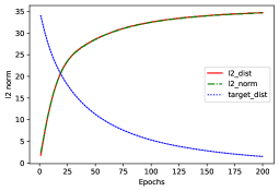
(a)

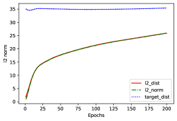
(b)

Figure 16: Norm of global model, distance to initialisation and distance to target, under attack by CGA. In particular, we see that the attack against $\ell_{2}^{2}$ is successful, as the distance between the global model and the target model goes to zero.

Appendix J Cifar-10 on VGG 13-BN Experiments

We considered VGG 13-BN, which was pretrained on cifar-10 by (Phan, 2021). We now assume that 10 users are given part of the cifar-10 database, while a strategic user also joins to the personalized federated gradient descent algorithm. The strategic user’s goal is to bias the global model towards a target model, which misclassifies the cifar-10 data, by reclassifying 0 into 1, 1 into 2… and 9 into 0.

J.1 Counter-Gradient Attack

We first show the result of performing counter-gradient attack on the last layer of the neural network. Essentially, images are now reduced to their vector embedding, and the last layer performs a simple linear classification akin to the case of MNIST (see Appendix I).

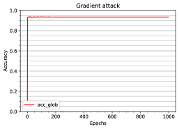
(a)

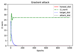
(b)

Figure 17: CGA on cifar-10.

J.2 Reconstructing a Model Attack

Reconstructing an attack model whose effect is equivalent to the counter-gradient attack is identical to what was done in the case of MNIST (see Section 5.2).

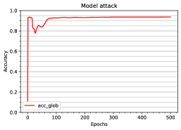
(a)

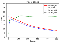
(b)

Figure 18: Model attack on cifar-10.

J.3 Reconstructing Data Poisoning

This last step is however nontrivial. On one hand, we could simply use the attack model to label a large number of random images. However, this solution would likely require a large sample complexity. For a more efficient data poisoning, we can construct vector embeddings on the indifference affine subspace $V$, as was done for MNIST in Section 5.3. This is what is shown below.

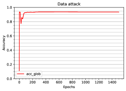
(a)

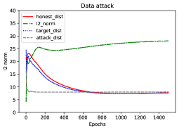
(b)

Figure 19: Data poisoning on cifar-10.

We acknowledge however that this does not quite correspond to data poisoning, as it requires reporting a vector embedding and its label, rather than an actual image and its label. The challenge is then to reconstruct an image that has a given vector embedding. We note that, while this is not a straightforward task in general, this has been shown to be at least somewhat possible for some neural networks, especially when they are designed to be interpretable (Zeiler & Fergus, 2014; Wang et al., 2019c; Mai et al., 2019).

Appendix K Single Data Poisoning for Least Square Linear Regression

Proof of Theorem 5.

We define the minimized loss with respect to $\rho$ and without strategic user $s$ by

$$\textsc{Loss}_{-s}^{*}(\rho,\vec{\mathcal{D}}_{-s})\triangleq\min_{\vec{\theta}_{-s}\in\mathbb{R}^{d\times(N-1)}}\left\{\sum_{n\neq s}\mathcal{L}_{n}(\theta_{n},\mathcal{D}_{n})+\sum_{n\neq s}\lambda\left\lVert{\theta_{n}-\rho}\right\rVert_{2}^{2}\right\}.$$ (175)

Now consider a subgradient $g\in\nabla_{\rho}\textsc{Loss}_{-s}^{*}(\theta^{\dagger}_{s},\vec{\mathcal{D}}_{-s})$ of the minimized loss at $\theta^{\dagger}_{s}$. For $x\triangleq\frac{-g}{2\lambda}$, then have $-g\in\nabla\left(\lambda\left\lVert{x}\right\rVert_{2}^{2}\right)$. We then define $\theta_{s}^{\spadesuit}\triangleq\theta^{\dagger}_{s}-x$.

$$0=g-g \in\nabla_{\rho}\textsc{Loss}_{-s}^{*}(\theta^{\dagger}_{s},\vec{\mathcal{D}}_{-s})+\nabla_{\rho}\left(\lambda\left\lVert{\theta_{s}^{\spadesuit}-\theta^{\dagger}_{s}}\right\rVert_{2}^{2}\right)$$ (176)

$$=\nabla_{\rho}\textsc{Loss}_{s}(\theta^{\dagger}_{s},\vec{\theta}^{*}_{-s}(\theta_{s}^{\spadesuit},\vec{\mathcal{D}}_{-s}),\theta_{s}^{\spadesuit},\vec{\mathcal{D}}_{-s}),$$ (177)

where $\textsc{Loss}_{s}$ is defined by (39). Now consider the data point $(\mathcal{Q},\mathcal{A})=(g,g^{T}\theta_{s}^{\spadesuit}-1)$. For $\mathcal{D}_{s}=\left\{(\mathcal{Q},\mathcal{A})\right\}$, we then have $\nabla\mathcal{L}_{s}(\theta_{s}^{\spadesuit},\mathcal{D}_{s})=g$, which implies

$$\nabla_{\theta_{s}}\textsc{Loss}{}(\theta^{\dagger}_{s},(\theta_{s}^{\spadesuit},\vec{\theta}^{*}_{-s}(\theta_{s}^{\spadesuit},\vec{\mathcal{D}}_{-s}),\vec{\mathcal{D}})=0.$$ (178)

Combining it all together with the uniqueness of the solution then yields

$$\operatorname*{arg\,min}_{(\rho,\vec{\theta})}\left\{\textsc{Loss}{}(\rho,\vec{\theta}{},\vec{\mathcal{D}})\right\}=\left(\theta^{\dagger}_{s},\left(\theta_{s}^{\spadesuit},\vec{\theta}^{*}_{-s}(\theta_{s}^{\spadesuit},\vec{\mathcal{D}}_{-s})\right)\right),$$ (179)

which is what we wanted. ∎

Appendix L Data Poisoning Against Linear Classification

L.1 Generating Efficient Poisoning Data and Initialization

For every label $a\in\left\{1,\ldots,9\right\}$, we define $y_{a}\triangleq\theta_{a}^{\spadesuit}-\theta_{0}^{\spadesuit}$, and $c_{a}\triangleq-(\theta_{a0}^{\spadesuit}-\theta_{00}^{\spadesuit})$ (where $\theta_{a0}^{\spadesuit}$ is the bias of the linear classifier). The indifference subspace $V$ is then the set of images $\mathcal{Q}\in\mathbb{R}^{d}$ such that $\mathcal{Q}^{T}y_{a}=c_{a}$ for all $a\in\left\{1,\ldots,9\right\}$.

To project any image $X\in\mathbb{R}^{d}$ on $V$, let us first construct an orthogonal basis of the vector space orthogonal to $V$, using the Gram-Schmidt algorithm. Namely, we first define $z_{1}\triangleq y_{1}$. Then, for any answer $a\in\left\{1,\ldots,9\right\}$, we define

$$z_{a}\triangleq y_{a}-\sum_{b<a}y_{a}^{T}z_{b}\frac{z_{b}}{\left\lVert{z_{b}}\right\rVert_{2}^{2}}.$$ (180)

It is easy to check that for $b<a$, we have $z_{a}^{T}z_{b}=0$. Moreover, if $\mathcal{Q}\in V$, then

$$z_{a}^{T}\mathcal{Q} =y_{a}^{T}\mathcal{Q}-\sum_{b<a}\frac{(y_{a}^{T}z_{b})(z_{b}^{T}\mathcal{Q})}{\left\lVert{z_{b}}\right\rVert_{2}^{2}}=c_{a}-\sum_{b<a}\frac{(y_{a}^{T}z_{b})(z_{b}^{T}\mathcal{Q})}{\left\lVert{z_{b}}\right\rVert_{2}^{2}}.$$ (181)

By induction, we see that $z_{a}^{T}\mathcal{Q}$ is a constant independent from $\mathcal{Q}$. Indeed, for $a=1$, this is clear as $z_{1}^{T}\mathcal{Q}=y_{1}^{T}\mathcal{Q}=c_{1}$. Moreover, for $a>1$, then, in the computation of $z_{a}^{T}\mathcal{Q}$, $\mathcal{Q}$ always appear as $z_{b}^{T}\mathcal{Q}$ for $b<a$. Moreover, denoting $c^{\prime}_{a}$ the constant such that $z_{a}^{T}\mathcal{Q}=c^{\prime}_{a}$ for all $a\in\left\{1,\ldots 9\right\}$, we see that these constants can be computed by

$$c^{\prime}_{a}=c_{a}-\sum_{b<a}\frac{y_{a}^{T}z_{b}}{\left\lVert{z_{b}}\right\rVert_{2}^{2}}c^{\prime}_{b}.$$ (182)

Finally, we can simply perform repeated projection onto the hyperplanes where $a$ is equally probable as the answer $0$. To do this, we first define the orthogonal projection $P(X,y,c)$ of $X\in\mathbb{R}^{d}$ on the hyperplane $x^{T}y=c$, which is given by

$$P(X,y,c)=X-(X^{T}y-c)\frac{y}{\left\lVert{y}\right\rVert_{2}^{2}}.$$ (183)

It is straightforward to verify that $P(X,y,c)^{T}y=c$ and that $P(P(X,y,c),y,c)=P(X,y,c)$. We then canonically define repeated projection by induction, as

$$P(X,(y_{1},\ldots,y_{k+1}),(c_{1},\ldots,c_{k+1}))\triangleq P(P(X,(y_{1},\ldots,y_{k}),(c_{1},\ldots,c_{k})),y_{k+1},c_{k+1}).$$ (184)

Now consider any image $X\in\mathbb{R}^{d}$. Its projection can be obtained by setting

$$\mathcal{Q}\triangleq P(X,(z_{1},\ldots,z_{9}),(c_{1}^{\prime},\ldots c_{9}^{\prime}))+\xi.$$ (185)

Note that to avoid being exactly on the boundary, and thus retrieve information about the scales of $\theta^{\spadesuit}$ and on which side of the boundary favors which label, we add a small noise $\xi$, to make sure $\mathcal{Q}$ does not lie exactly on $V$ (which would lead to multiple solutions for the learning), but small enough so that the probabilities of the different label remain close to $0.1$ (the equiprobable probability).

We acknowledge that images obtained this way may not be in $[0,1]^{d}$, like the images of the MNIST dataset. In general, one could search for points $\mathcal{Q}\in V\cap[0,1]^{d}$. Note that in theory, by Theorem 3 (or a generalization of it), labeling random images in $[0,1]^{d}$ should suffice. However, in the case where $V\cap[0,1]^{d}$ is empty, this procedure may require the labeling of significantly more images to be successful. This is discussed in more detail in Section L.3.

The convergence to the optimum is slow. But given that the problem is strictly convex, we focus here mostly on showing that the minimum is indeed a poisoned model. To boost the convergence, we initialize our learning algorithm at a point close to what we expect to be the minimum, by taking this minimum and adding a Gaussian noise, and then we observe the convergence to this minimum.

L.2 A Brief Theory of Data Poisoning for Linear Classification

Using the efficient poisoning data fabrication, we thus have a set of images $(\mathcal{Q},p(\mathcal{Q}))$, where $p_{a}(\mathcal{Q})$ is the probability assigned to image $\mathcal{Q}$ and label $a$. This defines the following local loss for the strategic user:

$$\mathcal{L}_{s}(\theta_{s},\mathcal{D}_{s})=\sum_{(\mathcal{Q},p(\mathcal{Q}))\in\mathcal{D}_{s}}\sum_{a\in\left\{0,1,\ldots,9\right\}}p_{a}(\mathcal{Q})\ln\sigma_{a}(\theta_{s},\mathcal{Q}),$$ (186)

where $\sigma_{a}(\theta_{s},\mathcal{Q})=\frac{\exp(\theta_{sa}^{T}\mathcal{Q}+\theta_{sa0})}{\sum\exp(\theta_{sb}^{T}\mathcal{Q}+\theta_{sb0})}$ is the probability that image $\mathcal{Q}$ has label $a$, according to the model $\theta_{s}$. We acknowledge that such labelings of queries is unusual. Evidently, in practice, an image may be labeled $N$ times, and the number of labels $N_{a}$ it received can be set to be approximately $N_{a}\approx Np_{a}(\mathcal{Q})$.

It is noteworthy that the gradient of the loss function is then given by

$$\left(\theta_{s}-\theta_{s}^{\spadesuit}\right)^{T}\nabla_{\theta_{s}}\mathcal{L}_{s}(\theta_{s},\mathcal{D}_{s})=\sum_{\mathcal{Q}\in\mathcal{D}_{s}}\sum_{a\in\left\{0,1,\ldots,9\right\}}\left(\sigma_{a}(\theta_{s},\mathcal{Q})-\sigma_{a}(\theta_{s}^{\spadesuit},\mathcal{Q})\right)\left(\theta_{sa}-\theta_{sa}^{\spadesuit}\right)^{T}\mathcal{Q}^{+},$$ (187)

where we defined $\mathcal{Q}^{+}\triangleq(1,\mathcal{Q})$ (which allows to factor in the bias of the model. This shows that $\nabla_{\theta_{s}}\mathcal{L}_{s}(\theta_{s},\mathcal{D}_{s})$ points systematically away from $\theta_{s}^{\spadesuit}$, and thus that gradient descent will move towards $\theta_{s}^{\spadesuit}$.

In fact, if the set of images $\mathcal{Q}$ cover all dimensions (which occurs if there are $\Omega(d)$ images, which is the case for 2,000 images, since $d=784$), then gradient descent will always move the model in the direction of $\theta_{s}^{\spadesuit}$, which will be the minimum. Moreover, by overweighting each data $(\mathcal{Q},p(\mathcal{Q}))$ by a factor $\alpha$ (as though the image $\mathcal{Q}$ was labeled $\alpha$ times), we can guarantee gradient-PAC* learning, which means that we will have $\theta_{s}^{*}\approx\theta_{s}^{\spadesuit}$, even in the personalized federated learning framework. This shows why data poisoning should work in theory, with relatively few data injections.

Note that the number of other users does make learning harder. Indeed, the gradient of the regularization $\mathcal{R}(\rho,\theta_{s})$ at $\rho=\theta_{s}^{\dagger}$ and $\theta_{s}=\theta_{s}^{\spadesuit}$ is equal to $2\lambda\left\lVert{\theta_{s}^{\dagger}-\theta_{s}^{\spadesuit}}\right\rVert_{2}$. As the number $N-1$ of other users grows, we should expect this distance to grow roughly proportionally to $N$. In order to make strategic user $s$ robustly learn $\theta_{s}^{\spadesuit}$, the norm of the gradient of the local loss $\mathcal{L}_{s}$ at $\theta_{s}^{\dagger}$ must be vastly larger than $2\lambda\left\lVert{\theta_{s}^{\dagger}-\theta_{s}^{\spadesuit}}\right\rVert_{2}$. This means that the value of $\alpha$ (or, equivalently, the number of data injected in $\mathcal{D}_{s}$) must also grow proportionally to $N$.

L.3 Data Poisoning Against MNIST with Images in $[0,1]^{d}$

Note that in the data poisoning attack depicted in Figure 2, poisoned data points are easily detectable, as they do not necessarily lie in $[0,1]^{d}$ like the pristine images of the MNIST dataset. However, this can be mitigated by the attacker with the cost of providing significantly more data points ($\sim 10^{5}$). For this, we conduct another experiment in which the attacker divides the poisoned images by the maximum value and clips negative values to 0 (to get images located in $[0,1]^{d}$). The results of this experiment are depicted in Figure 20.

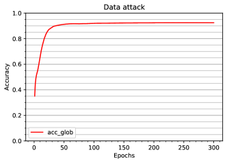
Figure 20: Accuracy of $\rho^{t}$ according to $\theta_{s}^{\dagger}$ (which relabels $0\rightarrow 1\rightarrow 2\rightarrow...\rightarrow 9\rightarrow 0$), under our data poisoning attack with poisoned images in $[0,1]^{d}$, with one attacker against two honest users.

References

- Acharya et al. (2022) Acharya, A., Hashemi, A., Jain, P., Sanghavi, S., Dhillon, I. S., and Topcu, U. Robust training in high dimensions via block coordinate geometric median descent. In Camps-Valls, G., Ruiz, F. J. R., and Valera, I. (eds.), International Conference on Artificial Intelligence and Statistics, AISTATS 2022, 28-30 March 2022, Virtual Event, volume 151 of Proceedings of Machine Learning Research, pp. 11145–11168. PMLR, 2022.
- Aghakhani et al. (2021) Aghakhani, H., Meng, D., Wang, Y.-X., Kruegel, C., and Vigna, G. Bullseye polytope: A scalable clean-label poisoning attack with improved transferability, 2021.
- Barreno et al. (2006) Barreno, M., Nelson, B., Sears, R., Joseph, A. D., and Tygar, J. D. Can machine learning be secure? In Proceedings of the 2006 ACM Symposium on Information, Computer and Communications Security, ASIACCS ’06, pp. 16–25, New York, NY, USA, 2006. Association for Computing Machinery. ISBN 1595932720. doi: 10.1145/1128817.1128824.
- Baruch et al. (2019) Baruch, G., Baruch, M., and Goldberg, Y. A little is enough: Circumventing defenses for distributed learning. In Wallach, H., Larochelle, H., Beygelzimer, A., d'Alché-Buc, F., Fox, E., and Garnett, R. (eds.), Advances in Neural Information Processing Systems, volume 32. Curran Associates, Inc., 2019.
- Ben-Porat & Tennenholtz (2017) Ben-Porat, O. and Tennenholtz, M. Best response regression. In Guyon, I., Luxburg, U. V., Bengio, S., Wallach, H., Fergus, R., Vishwanathan, S., and Garnett, R. (eds.), Advances in Neural Information Processing Systems, volume 30. Curran Associates, Inc., 2017.
- Bender et al. (2021) Bender, E. M., Gebru, T., McMillan-Major, A., and Shmitchell, S. On the dangers of stochastic parrots: Can language models be too big? In Elish, M. C., Isaac, W., and Zemel, R. S. (eds.), FAccT ’21: 2021 ACM Conference on Fairness, Accountability, and Transparency, Virtual Event / Toronto, Canada, March 3-10, 2021, pp. 610–623. ACM, 2021.
- Biggio et al. (2012) Biggio, B., Nelson, B., and Laskov, P. Poisoning attacks against support vector machines. In Proceedings of the 29th International Conference on Machine Learning, ICML 2012, Edinburgh, Scotland, UK, June 26 - July 1, 2012. icml.cc / Omnipress, 2012.
- Blanchard et al. (2017) Blanchard, P., Mhamdi, E. M. E., Guerraoui, R., and Stainer, J. Machine learning with adversaries: Byzantine tolerant gradient descent. In Guyon, I., von Luxburg, U., Bengio, S., Wallach, H. M., Fergus, R., Vishwanathan, S. V. N., and Garnett, R. (eds.), Advances in Neural Information Processing Systems 30: Annual Conference on Neural Information Processing Systems 2017, 4-9 December 2017, Long Beach, CA, USA, pp. 119–129, 2017.
- Blum et al. (2017) Blum, A., Haghtalab, N., Procaccia, A. D., and Qiao, M. Collaborative PAC learning. In Guyon, I., von Luxburg, U., Bengio, S., Wallach, H. M., Fergus, R., Vishwanathan, S. V. N., and Garnett, R. (eds.), Advances in Neural Information Processing Systems 30: Annual Conference on Neural Information Processing Systems 2017, December 4-9, 2017, Long Beach, CA, USA, pp. 2392–2401, 2017.
- Bradshaw & Howard (2019) Bradshaw, S. and Howard, P. N. The global disinformation order: 2019 global inventory of organised social media manipulation. Project on Computational Propaganda, 2019.
- Brown et al. (2020) Brown, T. B., Mann, B., Ryder, N., Subbiah, M., Kaplan, J., Dhariwal, P., Neelakantan, A., Shyam, P., Sastry, G., Askell, A., Agarwal, S., Herbert-Voss, A., Krueger, G., Henighan, T., Child, R., Ramesh, A., Ziegler, D. M., Wu, J., Winter, C., Hesse, C., Chen, M., Sigler, E., Litwin, M., Gray, S., Chess, B., Clark, J., Berner, C., McCandlish, S., Radford, A., Sutskever, I., and Amodei, D. Language models are few-shot learners. In Larochelle, H., Ranzato, M., Hadsell, R., Balcan, M., and Lin, H. (eds.), Advances in Neural Information Processing Systems 33: Annual Conference on Neural Information Processing Systems 2020, NeurIPS 2020, December 6-12, 2020, virtual, 2020.
- Cai et al. (2015) Cai, Y., Daskalakis, C., and Papadimitriou, C. H. Optimum statistical estimation with strategic data sources. In Grünwald, P., Hazan, E., and Kale, S. (eds.), Proceedings of The 28th Conference on Learning Theory, COLT 2015, Paris, France, July 3-6, 2015, volume 40 of JMLR Workshop and Conference Proceedings, pp. 280–296. JMLR.org, 2015.
- Chen et al. (2018a) Chen, J., Zhang, Q., and Zhou, Y. Tight bounds for collaborative PAC learning via multiplicative weights. In Bengio, S., Wallach, H. M., Larochelle, H., Grauman, K., Cesa-Bianchi, N., and Garnett, R. (eds.), Advances in Neural Information Processing Systems 31: Annual Conference on Neural Information Processing Systems 2018, NeurIPS 2018, December 3-8, 2018, Montréal, Canada, pp. 3602–3611, 2018a.
- Chen et al. (2018b) Chen, Y., Podimata, C., Procaccia, A. D., and Shah, N. Strategyproof linear regression in high dimensions. In Proceedings of the 2018 ACM Conference on Economics and Computation, EC ’18, pp. 9–26, New York, NY, USA, 2018b. Association for Computing Machinery. ISBN 9781450358293. doi: 10.1145/3219166.3219175.
- Chen et al. (2020) Chen, Y., Liu, Y., and Podimata, C. Learning strategy-aware linear classifiers. In Larochelle, H., Ranzato, M., Hadsell, R., Balcan, M. F., and Lin, H. (eds.), Advances in Neural Information Processing Systems, volume 33, pp. 15265–15276. Curran Associates, Inc., 2020.
- Collins et al. (2021) Collins, L., Hassani, H., Mokhtari, A., and Shakkottai, S. Exploiting shared representations for personalized federated learning. In Meila, M. and Zhang, T. (eds.), Proceedings of the 38th International Conference on Machine Learning, ICML 2021, 18-24 July 2021, Virtual Event, volume 139 of Proceedings of Machine Learning Research, pp. 2089–2099. PMLR, 2021.
- Dai et al. (2019) Dai, J., Chen, C., and Li, Y. A backdoor attack against lstm-based text classification systems. IEEE Access, 7:138872–138878, 2019.
- Dekel et al. (2010) Dekel, O., Fischer, F., and Procaccia, A. D. Incentive compatible regression learning. Journal of Computer and System Sciences, 76(8):759–777, 2010. ISSN 0022-0000. doi: https://doi.org/10.1016/j.jcss.2010.03.003.
- Dinh et al. (2020) Dinh, C. T., Tran, N. H., and Nguyen, T. D. Personalized federated learning with moreau envelopes. In Larochelle, H., Ranzato, M., Hadsell, R., Balcan, M., and Lin, H. (eds.), Advances in Neural Information Processing Systems 33: Annual Conference on Neural Information Processing Systems 2020, NeurIPS 2020, December 6-12, 2020, virtual, 2020.
- El-Mhamdi et al. (2020) El-Mhamdi, E., Guerraoui, R., Guirguis, A., Hoang, L. N., and Rouault, S. Genuinely distributed Byzantine machine learning. In Emek, Y. and Cachin, C. (eds.), PODC ’20: ACM Symposium on Principles of Distributed Computing, Virtual Event, Italy, August 3-7, 2020, pp. 355–364. ACM, 2020.
- El-Mhamdi et al. (2021a) El-Mhamdi, E., Farhadkhani, S., Guerraoui, R., Guirguis, A., Hoang, L. N., and Rouault, S. Collaborative learning in the jungle (decentralized, Byzantine, heterogeneous, asynchronous and nonconvex learning). In Advances in Neural Information Processing Systems 34: Annual Conference on Neural Information Processing Systems 2021, December 6-14, 2021, 2021a.
- El-Mhamdi et al. (2021b) El-Mhamdi, E., Farhadkhani, S., Guerraoui, R., and Hoang, L. N. Strategyproofness of the geometric median. CoRR, 2021b.
- El-Mhamdi et al. (2021) El-Mhamdi, E.-M., Guerraoui, R., and Rouault, S. Distributed momentum for Byzantine-resilient stochastic gradient descent. In 9th International Conference on Learning Representations, ICLR 2021, Vienna, Austria, May 4–8, 2021. OpenReview.net, 2021.
- Fallah et al. (2020) Fallah, A., Mokhtari, A., and Ozdaglar, A. E. Personalized federated learning with theoretical guarantees: A model-agnostic meta-learning approach. In Larochelle, H., Ranzato, M., Hadsell, R., Balcan, M., and Lin, H. (eds.), Advances in Neural Information Processing Systems 33: Annual Conference on Neural Information Processing Systems 2020, NeurIPS 2020, December 6-12, 2020, virtual, 2020.
- Farhadkhani et al. (2021) Farhadkhani, S., Guerraoui, R., and Hoang, L. Strategyproof learning: Building trustworthy user-generated datasets. CoRR, abs/2106.02398, 2021.
- Fedus et al. (2021) Fedus, W., Zoph, B., and Shazeer, N. Switch transformers: Scaling to trillion parameter models with simple and efficient sparsity. CoRR, abs/2101.03961, 2021.
- Fung & Garcia (2019) Fung, B. and Garcia, A. Facebook has shut down 5.4 billion fake accounts this year. CNN Business, 2019.
- Geiping et al. (2021) Geiping, J., Fowl, L. H., Huang, W. R., Czaja, W., Taylor, G., Moeller, M., and Goldstein, T. Witches’ brew: Industrial scale data poisoning via gradient matching. In International Conference on Learning Representations, 2021.
- Goodfellow et al. (2020) Goodfellow, I. J., Pouget-Abadie, J., Mirza, M., Xu, B., Warde-Farley, D., Ozair, S., Courville, A. C., and Bengio, Y. Generative adversarial networks. Commun. ACM, 63(11):139–144, 2020.
- Hanzely & Richtárik (2021) Hanzely, F. and Richtárik, P. Federated learning of a mixture of global and local models, 2021.
- Hanzely et al. (2020) Hanzely, F., Hanzely, S., Horváth, S., and Richtárik, P. Lower bounds and optimal algorithms for personalized federated learning. In Larochelle, H., Ranzato, M., Hadsell, R., Balcan, M., and Lin, H. (eds.), Advances in Neural Information Processing Systems 33: Annual Conference on Neural Information Processing Systems 2020, NeurIPS 2020, December 6-12, 2020, virtual, 2020.
- Hardt et al. (2016) Hardt, M., Megiddo, N., Papadimitriou, C., and Wootters, M. Strategic classification. In Proceedings of the 2016 ACM Conference on Innovations in Theoretical Computer Science, ITCS ’16, pp. 111–122, New York, NY, USA, 2016. Association for Computing Machinery. ISBN 9781450340571. doi: 10.1145/2840728.2840730.
- He et al. (2020) He, L., Karimireddy, S. P., and Jaggi, M. Byzantine-robust learning on heterogeneous datasets via resampling. CoRR, abs/2006.09365, 2020.
- Hoang (2020) Hoang, L. N. Science communication desperately needs more aligned recommendation algorithms. Frontiers in Communication, 5:115, 2020.
- Hoang et al. (2021) Hoang, L. N., Faucon, L., and El-Mhamdi, E. Recommendation algorithms, a neglected opportunity for public health. Revue Médecine et Philosophie, 4(2):16–24, 2021.
- Horn & Johnson (2012) Horn, R. A. and Johnson, C. R. Matrix Analysis. Cambridge University Press, 2 edition, 2012. doi: 10.1017/9781139020411.
- Huang et al. (2020) Huang, W. R., Geiping, J., Fowl, L., Taylor, G., and Goldstein, T. Metapoison: Practical general-purpose clean-label data poisoning. In Larochelle, H., Ranzato, M., Hadsell, R., Balcan, M., and Lin, H. (eds.), Advances in Neural Information Processing Systems 33: Annual Conference on Neural Information Processing Systems 2020, NeurIPS 2020, December 6-12, 2020, virtual, 2020.
- Ie et al. (2019) Ie, E., Jain, V., Wang, J., Narvekar, S., Agarwal, R., Wu, R., Cheng, H., Chandra, T., and Boutilier, C. Slateq: A tractable decomposition for reinforcement learning with recommendation sets. In Kraus, S. (ed.), Proceedings of the Twenty-Eighth International Joint Conference on Artificial Intelligence, IJCAI 2019, Macao, China, August 10-16, 2019, pp. 2592–2599. ijcai.org, 2019.
- Jain & Orlitsky (2020) Jain, A. and Orlitsky, A. A general method for robust learning from batches. In Larochelle, H., Ranzato, M., Hadsell, R., Balcan, M., and Lin, H. (eds.), Advances in Neural Information Processing Systems 33: Annual Conference on Neural Information Processing Systems 2020, NeurIPS 2020, December 6-12, 2020, virtual, 2020.
- Johnson & Diakopoulos (2021) Johnson, D. G. and Diakopoulos, N. What to do about deepfakes. Commun. ACM, 64(3):33–35, 2021.
- Kairouz et al. (2021) Kairouz, P., McMahan, H. B., Avent, B., Bellet, A., Bennis, M., Bhagoji, A. N., Bonawitz, K., Charles, Z., Cormode, G., Cummings, R., D’Oliveira, R. G. L., Eichner, H., Rouayheb, S. E., Evans, D., Gardner, J., Garrett, Z., Gascón, A., Ghazi, B., Gibbons, P. B., Gruteser, M., Harchaoui, Z., He, C., He, L., Huo, Z., Hutchinson, B., Hsu, J., Jaggi, M., Javidi, T., Joshi, G., Khodak, M., Konečný, J., Korolova, A., Koushanfar, F., Koyejo, S., Lepoint, T., Liu, Y., Mittal, P., Mohri, M., Nock, R., Özgür, A., Pagh, R., Raykova, M., Qi, H., Ramage, D., Raskar, R., Song, D., Song, W., Stich, S. U., Sun, Z., Suresh, A. T., Tramèr, F., Vepakomma, P., Wang, J., Xiong, L., Xu, Z., Yang, Q., Yu, F. X., Yu, H., and Zhao, S. Advances and open problems in federated learning, 2021.
- Karimireddy et al. (2021) Karimireddy, S. P., He, L., and Jaggi, M. Learning from history for Byzantine robust optimization. In Meila, M. and Zhang, T. (eds.), Proceedings of the 38th International Conference on Machine Learning, ICML 2021, 18-24 July 2021, Virtual Event, volume 139 of Proceedings of Machine Learning Research, pp. 5311–5319. PMLR, 2021.
- Konecný et al. (2015) Konecný, J., McMahan, B., and Ramage, D. Federated optimization: Distributed optimization beyond the datacenter. CoRR, abs/1511.03575, 2015.
- Konstantinov et al. (2020) Konstantinov, N., Frantar, E., Alistarh, D., and Lampert, C. On the sample complexity of adversarial multi-source PAC learning. In Proceedings of the 37th International Conference on Machine Learning, ICML 2020, 13-18 July 2020, Virtual Event, volume 119 of Proceedings of Machine Learning Research, pp. 5416–5425. PMLR, 2020.
- Kumar et al. (2020) Kumar, R. S. S., Nyström, M., Lambert, J., Marshall, A., Goertzel, M., Comissoneru, A., Swann, M., and Xia, S. Adversarial machine learning-industry perspectives. In 2020 IEEE Security and Privacy Workshops, SP Workshops, San Francisco, CA, USA, May 21, 2020, pp. 69–75. IEEE, 2020.
- Lehmann & Buschek (2021) Lehmann, F. and Buschek, D. Examining autocompletion as a basic concept for interaction with generative AI. i-com, 19(3):251–264, 2021.
- Mahloujifar et al. (2019) Mahloujifar, S., Mahmoody, M., and Mohammed, A. Data poisoning attacks in multi-party learning. In Chaudhuri, K. and Salakhutdinov, R. (eds.), Proceedings of the 36th International Conference on Machine Learning, ICML 2019, 9-15 June 2019, Long Beach, California, USA, volume 97 of Proceedings of Machine Learning Research, pp. 4274–4283. PMLR, 2019.
- Mai et al. (2019) Mai, G., Cao, K., Yuen, P. C., and Jain, A. K. On the reconstruction of face images from deep face templates. IEEE Trans. Pattern Anal. Mach. Intell., 41(5):1188–1202, 2019.
- McGuffie & Newhouse (2020) McGuffie, K. and Newhouse, A. The radicalization risks of GPT-3 and advanced neural language models. CoRR, abs/2009.06807, 2020.
- Meir et al. (2011) Meir, R., Almagor, S., Michaely, A., and Rosenschein, J. S. Tight bounds for strategyproof classification. In The 10th International Conference on Autonomous Agents and Multiagent Systems - Volume 1, AAMAS ’11, pp. 319–326, Richland, SC, 2011. International Foundation for Autonomous Agents and Multiagent Systems. ISBN 0982657153.
- Meir et al. (2012) Meir, R., Procaccia, A. D., and Rosenschein, J. S. Algorithms for strategyproof classification. Artificial Intelligence, 186:123–156, 2012. ISSN 0004-3702. doi: https://doi.org/10.1016/j.artint.2012.03.008.
- Mhamdi et al. (2018) Mhamdi, E. M. E., Guerraoui, R., and Rouault, S. The hidden vulnerability of distributed learning in byzantium. In Dy, J. G. and Krause, A. (eds.), Proceedings of the 35th International Conference on Machine Learning, ICML 2018, Stockholmsmässan, Stockholm, Sweden, July 10-15, 2018, volume 80 of Proceedings of Machine Learning Research, pp. 3518–3527. PMLR, 2018.
- Muñoz-González et al. (2017) Muñoz-González, L., Biggio, B., Demontis, A., Paudice, A., Wongrassamee, V., Lupu, E. C., and Roli, F. Towards poisoning of deep learning algorithms with back-gradient optimization. In Thuraisingham, B. M., Biggio, B., Freeman, D. M., Miller, B., and Sinha, A. (eds.), Proceedings of the 10th ACM Workshop on Artificial Intelligence and Security, AISec@CCS 2017, Dallas, TX, USA, November 3, 2017, pp. 27–38. ACM, 2017.
- Neudert et al. (2019) Neudert, L.-M., Howard, P., and Kollanyi, B. Sourcing and automation of political news and information during three european elections. Social Media+ Society, 5(3):2056305119863147, 2019.
- Nguyen & Zakynthinou (2018) Nguyen, H. L. and Zakynthinou, L. Improved algorithms for collaborative PAC learning. In Bengio, S., Wallach, H. M., Larochelle, H., Grauman, K., Cesa-Bianchi, N., and Garnett, R. (eds.), Advances in Neural Information Processing Systems 31: Annual Conference on Neural Information Processing Systems 2018, NeurIPS 2018, December 3-8, 2018, Montréal, Canada, pp. 7642–7650, 2018.
- Perote & Perote-Peña (2004) Perote, J. and Perote-Peña, J. Strategy-proof estimators for simple regression. Mathematical Social Sciences, 47(2):153–176, 2004. ISSN 0165-4896. doi: https://doi.org/10.1016/S0165-4896(03)00085-4.
- Perote & Sevilla (2003) Perote, J. and Sevilla, O. The impossibility of strategy-proof clustering. Economics Bulletin, 2003.
- Phan (2021) Phan, H. huyvnphan/pytorch_cifar10, January 2021.
- Qiao (2018) Qiao, M. Do outliers ruin collaboration? In Dy, J. G. and Krause, A. (eds.), Proceedings of the 35th International Conference on Machine Learning, ICML 2018, Stockholmsmässan, Stockholm, Sweden, July 10-15, 2018, volume 80 of Proceedings of Machine Learning Research, pp. 4177–4184. PMLR, 2018.
- Ricci et al. (2011) Ricci, F., Rokach, L., and Shapira, B. Introduction to recommender systems handbook. In Ricci, F., Rokach, L., Shapira, B., and Kantor, P. B. (eds.), Recommender Systems Handbook, pp. 1–35. Springer, 2011.
- Schwarzschild et al. (2021) Schwarzschild, A., Goldblum, M., Gupta, A., Dickerson, J. P., and Goldstein, T. Just how toxic is data poisoning? a unified benchmark for backdoor and data poisoning attacks. In Meila, M. and Zhang, T. (eds.), Proceedings of the 38th International Conference on Machine Learning, volume 139 of Proceedings of Machine Learning Research, pp. 9389–9398. PMLR, 18–24 Jul 2021.
- Severi et al. (2021) Severi, G., Meyer, J., Coull, S., and Oprea, A. Explanation-guided backdoor poisoning attacks against malware classifiers. In Bailey, M. and Greenstadt, R. (eds.), 30th USENIX Security Symposium, USENIX Security 2021, August 11-13, 2021, pp. 1487–1504. USENIX Association, 2021.
- Shafahi et al. (2018) Shafahi, A., Huang, W. R., Najibi, M., Suciu, O., Studer, C., Dumitras, T., and Goldstein, T. Poison frogs! targeted clean-label poisoning attacks on neural networks. In Bengio, S., Wallach, H. M., Larochelle, H., Grauman, K., Cesa-Bianchi, N., and Garnett, R. (eds.), Advances in Neural Information Processing Systems 31: Annual Conference on Neural Information Processing Systems 2018, NeurIPS 2018, December 3-8, 2018, Montréal, Canada, pp. 6106–6116, 2018.
- Shejwalkar et al. (2022) Shejwalkar, V., Houmansadr, A., Kairouz, P., and Ramage, D. Back to the drawing board: A critical evaluation of poisoning attacks on federated learning. In 2022 IEEE Symposium on Security and Privacy, 2022.
- Shum et al. (2018) Shum, H., He, X., and Li, D. From eliza to xiaoice: challenges and opportunities with social chatbots. Frontiers Inf. Technol. Electron. Eng., 19(1):10–26, 2018.
- Smith et al. (2013) Smith, J. R., Saint-Amand, H., Plamada, M., Koehn, P., Callison-Burch, C., and Lopez, A. Dirt cheap web-scale parallel text from the common crawl. In Proceedings of the 51st Annual Meeting of the Association for Computational Linguistics, ACL 2013, 4-9 August 2013, Sofia, Bulgaria, Volume 1: Long Papers, pp. 1374–1383. The Association for Computer Linguistics, 2013.
- Suya et al. (2021) Suya, F., Mahloujifar, S., Suri, A., Evans, D., and Tian, Y. Model-targeted poisoning attacks with provable convergence. In Meila, M. and Zhang, T. (eds.), Proceedings of the 38th International Conference on Machine Learning, ICML 2021, 18-24 July 2021, Virtual Event, volume 139 of Proceedings of Machine Learning Research, pp. 10000–10010. PMLR, 2021.
- Truong et al. (2020) Truong, L., Jones, C., Hutchinson, B., August, A., Praggastis, B., Jasper, R., Nichols, N., and Tuor, A. Systematic evaluation of backdoor data poisoning attacks on image classifiers. In 2020 IEEE/CVF Conference on Computer Vision and Pattern Recognition, CVPR Workshops 2020, Seattle, WA, USA, June 14-19, 2020, pp. 3422–3431. Computer Vision Foundation / IEEE, 2020.
- Valiant (1984) Valiant, L. G. A theory of the learnable. Commun. ACM, 27(11):1134–1142, 1984.
- Vershynin (2018) Vershynin, R. High-dimensional probability: An introduction with applications in data science, volume 47. Cambridge university press, 2018.
- Wainwright (2019) Wainwright, M. J. High-Dimensional Statistics: A Non-Asymptotic Viewpoint. Cambridge Series in Statistical and Probabilistic Mathematics. Cambridge University Press, 2019. doi: 10.1017/9781108627771.
- Wang et al. (2019a) Wang, A., Pruksachatkun, Y., Nangia, N., Singh, A., Michael, J., Hill, F., Levy, O., and Bowman, S. R. Superglue: A stickier benchmark for general-purpose language understanding systems. In Wallach, H. M., Larochelle, H., Beygelzimer, A., d’Alché-Buc, F., Fox, E. B., and Garnett, R. (eds.), Advances in Neural Information Processing Systems 32: Annual Conference on Neural Information Processing Systems 2019, NeurIPS 2019, December 8-14, 2019, Vancouver, BC, Canada, pp. 3261–3275, 2019a.
- Wang et al. (2019b) Wang, A., Singh, A., Michael, J., Hill, F., Levy, O., and Bowman, S. R. GLUE: A multi-task benchmark and analysis platform for natural language understanding. In 7th International Conference on Learning Representations, ICLR 2019, New Orleans, LA, USA, May 6-9, 2019. OpenReview.net, 2019b.
- Wang et al. (2019c) Wang, S., Wang, S., Zhang, X., Wang, S., Ma, S., and Gao, W. Scalable facial image compression with deep feature reconstruction. In 2019 IEEE International Conference on Image Processing, ICIP 2019, Taipei, Taiwan, September 22-25, 2019, pp. 2691–2695. IEEE, 2019c.
- Wu et al. (2020) Wu, Y., Ngai, E. W. T., Wu, P., and Wu, C. Fake online reviews: Literature review, synthesis, and directions for future research. Decis. Support Syst., 132:113280, 2020.
- Xie et al. (2019) Xie, C., Koyejo, O., and Gupta, I. Fall of empires: Breaking Byzantine-tolerant SGD by inner product manipulation. In Globerson, A. and Silva, R. (eds.), Proceedings of the Thirty-Fifth Conference on Uncertainty in Artificial Intelligence, UAI 2019, Tel Aviv, Israel, July 22-25, 2019, volume 115 of Proceedings of Machine Learning Research, pp. 261–270. AUAI Press, 2019.
- Yang & Li (2021) Yang, Y. and Li, W. BASGD: buffered asynchronous SGD for Byzantine learning. In Meila, M. and Zhang, T. (eds.), Proceedings of the 38th International Conference on Machine Learning, ICML 2021, 18-24 July 2021, Virtual Event, volume 139 of Proceedings of Machine Learning Research, pp. 11751–11761. PMLR, 2021.
- Yin et al. (2018) Yin, D., Chen, Y., Ramchandran, K., and Bartlett, P. L. Byzantine-robust distributed learning: Towards optimal statistical rates. In Dy, J. G. and Krause, A. (eds.), Proceedings of the 35th International Conference on Machine Learning, ICML 2018, Stockholmsmässan, Stockholm, Sweden, July 10-15, 2018, volume 80 of Proceedings of Machine Learning Research, pp. 5636–5645. PMLR, 2018.
- Zeiler & Fergus (2014) Zeiler, M. D. and Fergus, R. Visualizing and understanding convolutional networks. In Fleet, D. J., Pajdla, T., Schiele, B., and Tuytelaars, T. (eds.), Computer Vision - ECCV 2014 - 13th European Conference, Zurich, Switzerland, September 6-12, 2014, Proceedings, Part I, volume 8689 of Lecture Notes in Computer Science, pp. 818–833. Springer, 2014.
- Zhao et al. (2020) Zhao, S., Ma, X., Zheng, X., Bailey, J., Chen, J., and Jiang, Y. Clean-label backdoor attacks on video recognition models. In 2020 IEEE/CVF Conference on Computer Vision and Pattern Recognition, CVPR 2020, Seattle, WA, USA, June 13-19, 2020, pp. 14431–14440. Computer Vision Foundation / IEEE, 2020.
- Zhu et al. (2019) Zhu, C., Huang, W. R., Li, H., Taylor, G., Studer, C., and Goldstein, T. Transferable clean-label poisoning attacks on deep neural nets. In Chaudhuri, K. and Salakhutdinov, R. (eds.), Proceedings of the 36th International Conference on Machine Learning, ICML 2019, 9-15 June 2019, Long Beach, California, USA, volume 97 of Proceedings of Machine Learning Research, pp. 7614–7623. PMLR, 2019.