Local Differential Privacy for Belief Functions

Abstract

In this paper, we propose two new definitions of local differential privacy for belief functions. One is based on Shafer’s semantics of randomly coded messages and the other from the perspective of imprecise probabilities. We show that such basic properties as composition and post-processing also hold for our new definitions. Moreover, we provide a hypothesis testing framework for these definitions and study the effect of “don’t know" in the trade-off between privacy and utility in discrete distribution estimation.

1 Introduction

Differential privacy (DP) is a mathematically rigorous definition of privacy which addresses the paradox of learning nothing about an individual while learning useful information about a population [12, 13]. In particular, local differential privacy (LDP) is a model of differential privacy with the added restriction that even if an adversary has access to the personal responses of an individual in the database, that adversary will still be unable to learn too much about the user’s personal data [22, 20, 10]. The uncertainty in standard LDP mechanisms is usually provided by randomization which associates each input with a probability function over all possible outputs. The prototypical example of an LDP mechanism is the randomized response survey technique proposed in [35]. Current randomized response mechanisms equate privacy-preserving with lying and are designed on the assumption that users abide by the data collection protocol which allows respondents to lie with a known probability. However, recent research results from the perspective of the respondents show that, in practice, although these mechanisms allow the respondents to maintain privacy, the procedures may confuse respondents, fail to address the concerns of the users and hence yield nonresponse or noncompliance [37, 4, 29]. An effective differential privacy communication can increase data-sharing rates [37].

To address noncompliance and nonresponse, we propose in this paper to design differential privacy mechanisms which incorporate “don’t know" or nonresponse as an alternative outcome or allow imprecision in the mechanism design. In practice, people may prefer not to response or say “I don’t know" to withhold sensitive information which minimizes the questionable ethical consequences of lying in their eyes [3]. By addressing such ethical privacy concerns, our new mechanisms aims to increase respondents’ willing to share their data. Here we study this new type of privacy mechnisms from a more general Dempster-Shafer perspective by representing uncertainty in privacy mechanisms with belief functions [6, 30]. The Dempster-Shafer theory (also known as the theory of evidence or the theory of belief functions) is a well-known uncertainty theory for its expressiveness in representing ignorance. The theory improves the root concepts of probabilities “yes" and “no" that sum to one, by appending a third probability of “don’t know" [7]. As the world of statistical analysis moves more and more to “big data" and associated “complex systems", the Dempster-Shafer theory provides a middle ground with the third probability “don’t know" and can be expected to become increasingly important in privacy protection.

Our first and main contribution in this paper is to propose two new definitions of LDP (one is $\epsilon$-local differential privacy according to Shafer ($\epsilon$-SLDP) (Definition 3.1) and the other according to Walley ($\epsilon$-WLDP) (Definition 3.13)) and to provide a statistical framework for these two definitions as the trade-offs between type I and II errors in a natural hypothesis-testing problem (Theorems 3.5 and 3.18). Our second contribution is to characterize the effect of “don’t know" in the trade-off between privacy and utility in discrete distribution estimation problem. The privacy mechanisms in the two definitions associate each input $x$ with a belief function on the output set $Y$. The difference between these two definitions comes from their different semantics of belief functions. The first definition is motivated by Shafer’s interpretation of belief functions as randomly coded messages [32]. In this semantics, we generalize Warner’s randomized response mechanism by allowing answering “don’t know" with probability $1-p-q$ where $p$ is the probability of answering truthfully and $q$ the probability of lying. For the discrete distribution estimation problem of a generalized Warner’s model, we study the effect of “don’t know" on the trade-off between the privacy loss and the estimation accuracy. The most important and difficult step is to compute the variance of the maximum likelihood estimation of the parameter $\pi$, the true proportion of the people with the sensitive property. We employ some combinatorial techniques to obtain a formula for the estimation accuracy (Theorem 3.10). We show that, when the probability of “don’t know" increases, the overall effect of the trade-off for this generalized model decreases, and when this probability equals 0, the effect is optimal and the trade-off is the same as that for the standard Warner’s model (Figure 2). In the second definition, we adopt the imprecise-probability semantics to accommodate unknown response probabilities in privacy mechanisms and interpret belief function $bel$ as the set of all probability functions $pr$ which are consistent with $bel$ [33]. Both the privacy loss and estimation accuracy are defined with respect to those consistent probability functions according to the worst-case analysis. Moreover, we compare the trade-offs between privacy and estimation accuracy for these two definitions ($\epsilon$-SLDP and $\epsilon$-WLDP) and Warner’s randomized response mechanism (Figure 5).

2 Dempster-Shafer Theory

Let $\Omega$ be a frame and $\mathcal{A}=2^{\Omega}$ be the Boolean algebra of propositions. $|A|$ denotes the cardinality of a subset $A$. A mass assignment (or mass function) over $\Omega$ is a mapping $m:\mathcal{A}\rightarrow[0,1]$ satisfying $\sum_{A\in\mathcal{A}}m(A)=1$. A mass function $m$ is called normal if $m(\emptyset)=0$. A belief function is a function $bel:\mathcal{A}\rightarrow[0,1]$ satisfying the conditions: $bel(\emptyset)=0$, $bel(\Omega)=1$ and $bel(\bigcup_{i=1}^{n}A_{i})\geq\sum_{\emptyset\neq I\subseteq\{1,\cdots,n\}}(-1)^{|I|+1}bel(\cap_{i\in I}A_{i})$ where $A_{i}\in\mathcal{A}$ for all $i\in\{1,\cdots,n\}$. A mapping $f:\mathcal{A}\rightarrow[0,1]$ is a belief function if and only if its Möbius transform is a mass assignment (Page 39 in [30]). In other words, if $m:\mathcal{A}\rightarrow[0,1]$ is a mass assignment, then it determines a belief function $bel:\mathcal{A}\rightarrow[0,1]$ as follows: $bel(A)=\sum_{B\subseteq A}m(B)$ for all $A\in\mathcal{A}$. Moreover, given a belief function $bel$, we can obtain its corresponding mass function $m$ as follows: $m(A)=\sum_{B\subseteq A}(-1)^{|A\setminus B|}bel(B)\text{ for all }A\in\mathcal{A}.$ Intuitively, for a subset event $A$, $m(A)$ measures the belief that an agent commits exactly to $A$, not the total belief $bel(A)$ that an agent commits to $A$. A subset $A$ with non-zero mass is called a focal set. The belief function $bel$ is called Bayesian if $m(A)=0$ for all non-singletons $A$. The corresponding plausibility function $pl_{m}:2^{\Omega}\rightarrow[0,1]$ is defined by $pl_{m}(A)=\sum_{E\cap A\neq\emptyset}m(E)$ for all $A\subseteq\Omega$. Whenever the context is clear, we drop the subscript $m$. For $m,bel$ and $pl$, if we know any one of them, then we can determine the other two. Without further notice, all mass functions in this paper are assumed to be normal and all subsets are focal.

In this paper, we focus on only two semantics of belief functions. The first one is Shafer’s semantics of belief functions in terms of randomly coded messages. Suppose someone chooses a code at random from a list of codes, uses the code to encode a message, and then sends us the result. We know the list of codes and the chance of each code being chosen–say the list is $c_{1},\cdots,c_{n}$, and the chance of $c_{i}$ being chosen is $p_{i}$. We decode the encoded message using each of the codes and find that this always produces a message of the form “the truth is in A" for some non-empty subset $A$ of the set of possibilities $\Omega$. Let $A_{i}$ denote the subset we get when we decode using $c_{i}$, and set $m(A)=\sum\{p_{i}:1\leq i\leq n,A_{i}=A\}$ for each $A\subseteq\Omega$. The number $m(A)$ is the sum of the chances for those codes that indicate A was the true message; it is, in a sense, the total chance that the true message was $A$. Notice that $m(\emptyset)=0$ and that the $m(A)$ sum to one. The quantity $bel(A)=\sum_{B\subseteq A}m(B)$ is, in a sense, the total chance that the true message implies $A$. If the true message is infallible and the coded message is our only evidence, then it is natural to call $bel(A)$ our probability or degree of belief that the truth lies in $A$. The second interpretation of belief functions in this paper is from the perspective of imprecise probabilities. Given a belief function $bel$, let $\mathcal{P}_{bel}$ denote the set of all probability functions which are consistent with or dominate over $bel$. In other words, $\mathcal{P}_{bel}=\{pr:pr\text{ is a probability function on }\Omega$ and $pr\geq bel\}$ where $pr\geq bel$ means $pr(E)\geq bel(E)$ for all $E\subseteq\Omega$. Due to lack of information, uncertainty can’t be represented by a probability function but by a belief function $bel$. All consistent probability functions are possible. Whenever enough information is available, we may specify a probability function from $\mathcal{P}_{bel}$ to represent the uncertainty. One may refer to [5] and [13] for a detailed introduction to belief functions and DP.

3 Local Differential Privacy

Let $X$ be a private source of information defined on a discrete, finite input alphabet $X=\{x_{1},\cdots,x_{k}\}$ and $Y$ be an output alphabet $Y=\{y_{1},\cdots,y_{l}\}$ that need not be identical to the input alphabet $X$. In this paper, we will represent a privacy mechanism $Q$ via a row-stochastic matrix. For simplicity, we also use $Q$ to denote this matrix. $Q$ is called an evidential privacy mechanism if each row of the matrix $Q$ is a mass function on $Y$. In other words, each evidential privacy mechanism $Q$ maps $X=x$ to $Y\in E$ with $Q(x)$ which can be represented by a mass $m^{Q}_{x}(E)$ (belief $bel^{Q}_{x}(E)$ or plausibility $pl^{Q}_{x}(E)$) where $m^{Q}_{x}$ ($bel^{Q}_{x}(E)$ or $pl^{Q}_{x}(E)$) is a mass (belief or plausibility) function on $Y$ for all $x\in X$. Since $m_{x}^{Q}(\emptyset)=0$ for all $x$, we write the mechanism $Q$ as a $k\times(2^{l}-1)$ matrix. Whenever the context is clear, we usually drop the superscript $Q$. In this paper, we assume that all the alphabet sets are finite. In other words, an evidential privacy mechanism is just a standard LDP mechanism whose instructions are defined by random sets instead of probability functions.

3.1 LDP according to Shafer

For an evidential privacy mechanism $Q$, let $r^{Q}_{S}=max_{x,x^{\prime}\in X,E\subseteq Y}\frac{m_{x}^{Q}(E)}{m_{x^{\prime}}^{Q}(E)}$ and $\epsilon^{Q}_{S}=ln(r^{Q}_{S})$.

Definition 3.1

For any $\epsilon>0$, the mechanism $Q$ is called $\epsilon$-locally differential private according to Shafer ($\epsilon$-SLDP for short) if $-\epsilon\leq\epsilon^{Q}_{S}\leq\epsilon$. And $\epsilon^{Q}_{S}$ is called the privacy loss of $Q$ according to Shafer and $\epsilon$ is a privacy budget. $\lhd$

In other words, by observing $E$, the adversary cannot reliably infer whether $X=x$ or $X=x^{\prime}$ (for any pair $x$ and $x^{\prime}$). Indeed, the smaller the $\epsilon$ is, the closer the likelihood ratio of $X=x$ to $X=x^{\prime}$ is to 1. Therefore, when $\epsilon$ is small, the adversary cannot recover the true value of $X$ reliably. In this definition, we adopt Shafer’s interpretation as randomly coded messages. Each subset of $Y$ is treated as an individual message or response. The mechanism randomly chooses a code $c$ and uses it to encode a message $E\subseteq Y$. And $m_{x}(E)$ is equal to the chance of choosing $c$. If we set $2^{Y}\setminus\{\emptyset\}$ as the output alphabet, then the above $Q$ is simply the standard local differential private mechanism. In particular, if each row of $Q$ is Bayesian, then $Q$ is essentially a standard randomized mechanism and the $\epsilon$-SLDP is just the standard $\epsilon$-$LDP$ for randomized privacy mechanisms. Almost all basic properties for privacy-preserving randomized mechanisms can be generalized to the setting of belief functions. Let $r^{Q}_{pl,S}=max_{x,x^{\prime}\in X,E\subseteq Y}\frac{pl_{x}^{Q}(E)}{pl_{x^{\prime}}^{Q}(E)}$ and $r^{Q}_{bel,S}=max_{x,x^{\prime}\in X,E\subseteq Y}\frac{bel_{x}^{Q}(E)}{bel_{x^{\prime}}^{Q}(E)}$. Denote $\epsilon^{Q}_{pl,S}:=ln(r^{Q}_{pl,S})$ and $\epsilon^{Q}_{bel,S}:=ln(r^{Q}_{bel,S})$.

Lemma 3.2

If privacy mechanism $Q$ is $\epsilon$-$SLDP$, then $-\epsilon\leq\epsilon^{Q}_{bel,S}\leq\epsilon$ and $-\epsilon\leq\epsilon^{Q}_{pl,S}\leq\epsilon$.

From Lemma 3.2, we know that $\epsilon^{Q}_{S}\geq\epsilon^{Q}_{pl,S}$. But generally we don’t have the converse that $\epsilon^{Q}_{pl,S}\geq\epsilon^{Q}_{S}$. If we have several building blocks for designing differentially private algorithms, it is important to understand how we can combine them to design more sophisticated algorithms.

Lemma 3.3

(Composition) Let $Q_{1}$ be an $\epsilon_{1}$-SLDP evidential privacy mechanism from $X$ to $Y_{1}$ and $Q_{2}$ be an $\epsilon_{2}$-SLDP evidential privacy mechanisms from $X$ to $Y_{2}$. Then their combination $Q_{1,2}$ defined by $Q_{1,2}(x)=(Q_{1}(x),Q_{2}(x))$ is $\epsilon_{1}+\epsilon_{2}$-SLDP.

The composition of a data-independent mapping $f$ with an $\epsilon$ locally differential private algorithm $Q$ is also $\epsilon$ locally differential private.

Lemma 3.4

(Post-processing) Let $Q$ be an $\epsilon$-SLDP mechanism from $X$ to $Y$ and $f$ is a randomized algorithm from $Y$ to another finite alphabet set $Z$. Then $f\circ Q$ is an $\epsilon$-SLDP mechanism from $X$ to $Z$.

Now we offer a hypothesis testing interpretation for the above $\epsilon$-$SLDP$. From an attacker’s perspective, the privacy requirement can be formalized as the following hypothesis testing problem for two datasets $x$ and $x^{\prime}$:

$H_{0}$: the underlying dataset is $x$ vs. $H_{1}$: the underlying dataset is $x^{\prime}$.

The output of the mechanism $Q$ serves as the basis for performing the hypothesis testing problem. The distinguishability of the two inputs $x$ and $x^{\prime}$ can be translated into the trade-off between type I and type II errors [9]. For belief functions, it is natural to consider minimax tests [18]. Formally, consider a rejection rule $\varphi:Y\rightarrow[0,1]$. Let $\mathcal{P}_{x}^{Q}$ and $\mathcal{P}_{x^{\prime}}^{Q}$ denote the two sets of probability functions dominating $bel^{Q}_{x}$ and $bel^{Q}_{x^{\prime}}$ respectively. In other words, $\mathcal{P}_{x}^{Q}=\{pr\in\Delta(Y):pr\geq bel_{x}^{Q}\}$ and $\mathcal{P}_{x^{\prime}}^{Q}=\{pr\in\Delta(Y):pr\geq bel_{x^{\prime}}^{Q}\}$. The lower power of $\varphi$ under $x^{\prime}$ is defined as $\pi_{x^{\prime}}:=\text{inf}_{pr\in\mathcal{P}^{Q}_{x^{\prime}}}\mathbb{E}_{pr}(\varphi)$. In the setting of $\epsilon$-$SLDP$, we assume that type I error $\alpha_{\varphi}$ is represented by $\text{sup}_{pr\in\mathcal{P}^{Q}_{x}}\mathbb{E}_{pr}(\varphi)$ and type II error by $\beta_{\varphi}=1-\text{inf}_{pr\in\mathcal{P}^{Q}_{x^{\prime}}}\mathbb{E}_{pr}(\varphi)$. A test $\varphi$ is called a level-$\alpha$ minimax test if $\varphi=argmin\{\beta_{\varphi}:\alpha_{\varphi}\leq\alpha\}$. The following theorem is a generalization of the well-known result (Theorem 2.4 in [36]) for standard differential privacy.

Theorem 3.5

For any evidential privacy mechanism $Q$, the following two statements are equivalent:

1. $Q$ is $\epsilon$-SLDP;

2. If type I error $\alpha_{\varphi}\in[l,L]$, then type II error $\beta_{\varphi}\in[u(L),U(l)]$ where $u(\alpha):=max\{e^{-\epsilon}(1-\alpha),1-\alpha e^{\epsilon}\}$ and $U(\alpha):=min\{e^{\epsilon}(1-\alpha),1-\alpha e^{-\epsilon}\}$.

Now we consider the hypothesis testing problem for the composition and would like to distinguish between $Q(x)\times Q(x)$ and $Q(x^{\prime})\times Q(x^{\prime})$. The corresponding type I and II errors $\alpha^{2}_{\varphi}$ and $\beta^{2}_{\varphi}$ can be defined similarly. For simplicity, we only show the two-fold composition and other multi-fold compositions can be obtained similarly.

Corollary 3.6

For the hypothesis testing problem for the composition, if type I error $\alpha^{2}_{\varphi}\in[l,L]$, then type II error $\beta^{2}_{\varphi}\in[u^{2}(L),U^{2}(l)]$ where $u^{2}(\alpha):=max\{e^{-2\epsilon}(1-\alpha),-\alpha+\frac{2}{e^{\epsilon}+1},1-\alpha e^{2\epsilon}\}$ and $U^{2}(\alpha):=min\{e^{2\epsilon}(1-\alpha),1-\alpha e^{-2\epsilon},-\alpha+\frac{3-e^{-2\epsilon}}{e^{\epsilon}+1}\}$.

Both Theorem 3.5 and Corollary 3.6 can be visualized in Figure 1.

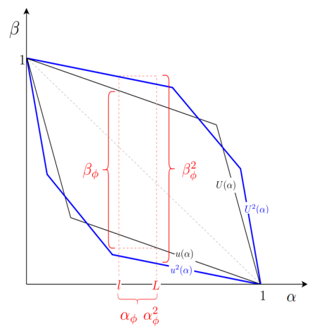
Figure 1: Trade-off between type I and II errors for SLDP

The discrete estimation problem is defined as follows. Given a prior which is a vector $\pi=(\pi_{1},\dots,\pi_{k})$ on the probability simplex $\mathbb{S}^{k}=\{p=(\pi_{1},\dots,\pi_{k}):\pi_{i}\geq 0(1\leq i\leq k),\sum_{i=1}^{k}\pi_{i}=1\}$, samples $X_{1},\cdots,X_{n}$ are drawn i.i.d. according to $\pi$. A privacy mechanism $Q$ is then applied independently to each sample $X_{i}$ to produce $Y^{n}=(Y_{1};\cdots,Y_{n})$, the sequence of private observations. Observe that the $Y_{i}$’s are distributed according to $m=\pi Q$, which are mass functions not necessarily probability functions when $Q$ is evidential. Our goal is to estimate the distribution vector $\pi$ from $Y^{n}$ within a certain privacy budget requirement. The performance of the estimation may be measured via a loss function. Here we use the mean square loss function. $Q$ is called optimal if the estimation error is the smallest. A classic example for discrete distribution estimation is Warner’s randomized response method for survey research [35].

Example 3.7

According to prototypical Warner’s randomized response mechanism $Q_{W}$, the respondent answers truthfully with probability $p$ and lies with probability $1-p$. Let $\pi$ be the true proportion of the people having property $P$. A sample of $Y_{1},\cdots,Y_{n}$ of respondents are drawn with replacement from the population and their responses are distributed i.i.d. according to $(q_{1},q_{2})=(\pi,1-\pi)Q_{W}$. So $q_{1}=\pi p+(1-\pi)(1-p)$ and $q_{2}=\pi(1-p)+(1-\pi)p$. Arrange the indexing of the sample so that the first $n_{1}$ respondents say "Yes" and the remaining $n-n_{1}$ answers "No". We obtain the maximum likelihood estimation of $\pi$ as $\hat{\pi}=\frac{p-1}{2p-1}+\frac{n_{1}}{(p-1)n}$. It can be shown [35, 16] that this distribution estimation $\hat{\pi}$ is unbiased and its mean square error or variance is the following formula:

$$Var[\hat{\pi}] =\frac{-(\pi-\frac{1}{2})^{2}+\frac{1}{4}}{n}+\frac{\frac{1}{4(2p-1)^{2}}-\frac{1}{4}}{n}$$ (1)

Within the privacy budget of $\epsilon$, the optimal privacy mechanism is

$$Q_{WRR}=\frac{1}{e^{\epsilon}+1}\left(\begin{array}[]{cc}e^{\epsilon}&1\\ 1&e^{\epsilon}\end{array}\right).$$

Now we are generalizing the above Warner’s model by allowing a third response “I don’t know" and representing the corresponding uncertainty with a mass function. Let $Q_{2\times 3}$ denote a known row-stochastic matrix as follows:

$$Q_{2\times 3}=\left(\begin{array}[]{ccc}p&q&1-p-q\\ q&p&1-p-q\end{array}\right)$$

where $p,q\in[0,1]$. $Q_{2\times 3}$ may be regarded as a generalized Warner’s randomized response mechanism where a respondent answers truthfully with probability $p$, tells a lie with $q$ and don’t respond or respond "I don’t know" with probability $1-p-q$. We may assume in this paper that $p>\frac{1}{2}$.

Remark 3.8

In the following we choose to work with such a simple form $Q_{2\times 3}$ of LDP for belief functions. A more general form can be studied similarly, but unfortunately we couldn’t obtain closed forms for (approximate) estimation and error as we achieve below for this simple form $Q_{2\times 3}$. The maximum likelihood estimation problem for the more general form can be naturally formalized as a mixture of the conditional mass functions associated with the evidential privacy mechanism with the mixture proportions as the unknown prior distribution of the sensitive population.We can apply EM algorithm to approximate the prior distribution and compute its Fisher information and further the standard error of the approximation [1]. However, the simple form provides us with a neat formula of estimation error (Theorem 3.10) and hence a formula for the privacy-utility trade-off. Indeed the simple form for evidential mechanism is enough to illustrate the effect of the answer “I don’t know" or nonresponse on the privacy-utility trade-off. Both the simulation experiments and Figure 2 afterwards are based on the above analysis. In this paper we mainly focus on this simple form $Q_{2\times 3}$. But we expect that such a simple form to evidential privacy mechanisms is the same as Warner’s $2\times 2$ mechanism to the standard LDP. For standard LDP, every approximate DP algorithm can be simulated by a (leaky) variant of Warner’s $2\times 2$ mechanism (a well-known result in optimal composition [28, 21]). From a broader and deeper perspective, we believe that every approximate evidential privacy mechanism can be simulated by some variant of our $2\times 3$ mechanisms in this paper. In this sense, our contribution is similar to Warner’s contribution to standard LDP.

A simple random sample of $n$ people is drawn with replacement from the population. Let $Z_{i}$ denote the $i$-th sample element. Recall that $\pi$ is the true proportion of the people with the sensitive property $P$. $Z_{i}$ is distributed according to the following $(q_{1},q_{2},q_{3})$:

$$\left(\begin{array}[]{ccc}q_{1}&q_{2}&q_{3}\end{array}\right)=\left(\begin{array}[]{ccc}\pi&1-\pi\end{array}\right)\left(\begin{array}[]{ccc}p&q&1-p-q\\ q&p&1-p-q\end{array}\right)$$

In other words, $q_{1}=\pi p+(1-\pi)q$, $q_{2}=\pi q+(1-\pi)p$, and $q_{3}=1-p-q$. Note that $q_{1}+q_{2}+q_{3}=1$. It implies that $Z_{i}$ says “Yes", “No" and “don’t know" with probabilities $q_{1},q_{2}$ and $q_{3}$ respectively. Arrange the indexing of the sample so that the first $n_{1}$ sample elements say $Yes$, the next $n_{2}$ say $No$ and the last $n_{3}$ say “don’t know" where $n_{1},n_{2}$ and $n_{3}$ are natural numbers such that $n_{1}+n_{2}+n_{3}=n$. So the likelihood of the sample is $L(\pi)=q_{1}^{n_{1}}q_{2}^{n_{2}}q_{3}^{n_{3}}$. By taking its logarithm and then setting its derivative to be zero, we obtain $\frac{n_{1}}{q_{1}}-\frac{n_{2}}{q_{2}}=0$. So we obtain the maximum likelihood estimation (MLE) of $\pi$ as follows:

$$\hat{\pi} =\frac{n_{2}q-n_{1}p}{(n_{1}+n_{2})(q-p)}.$$ (2)

Now we want to compute the expectation of $\hat{\pi}$. From $Z_{i}$, we define three new random variables $Z_{i1}=\mathbb{I}_{[Z_{i}=Yes]},Z_{i2}=\mathbb{I}_{[Z_{i}=No]}$ and $Z_{i3}=\mathbb{I}_{[Z_{i}=\text{don't know}]}$ (where $\mathbb{I}$ denotes the indicator function). Then $Z_{i}=Z_{i1}+Z_{i2}+Z_{i3},N_{1}=\sum_{i=1}^{n}Z_{i1},N_{2}=\sum_{i=1}^{n}Z_{i2}$ and $N_{3}=\sum_{i=1}^{n}Z_{i3}$. So $N_{1}+N_{2}+N_{3}=n$. We obtain the conditional expectation of the MLE.

Theorem 3.9

$\mathbb{E}[\frac{N_{2}q-N_{1}p}{(N_{1}+N_{2})(q-p)}|N_{1}+N_{2}\neq 0]=\pi$.

Theorem 3.10

$Var(\hat{\pi}|N_{1}+N_{2}\neq 0)=\frac{1}{(q-p)^{2}}[\pi p+(1-\pi)q][\pi q+(1-\pi)p]A=[-(\pi-\frac{1}{2})^{2}+\frac{1}{4}(\frac{p+q}{p-q})^{2}]A$ where $A=\sum_{0\leq N_{3}<n}\frac{1}{n-N_{3}}$ ${n}\choose{N_{3}}$$(1-q_{3})^{n-N_{3}}q_{3}^{N_{3}}$.

The formula in Theorem 3.10 is essential to our analysis of the trade-off between privacy loss and estimation accuracy. One may refer to the supplementary materials for a detailed proof (of independent interest). In this paper, we adopt from [14] a good approximation of $A$ as $\frac{1}{(n+1)(p+q)-1}$. In particular, with this approximation, when $p+q=1$, $Var[\hat{\pi}|N_{1}+N_{2}\neq 0]=\frac{-(\pi-\frac{1}{2})^{2}+\frac{1}{4}\frac{1}{(2p-1)^{2}}}{n}$, which is exactly the estimation error of Warner’s model ( Eq. (1)).

Corollary 3.11

Let $f(q)=\frac{-(\pi-\frac{1}{2})^{2}+\frac{1}{4}(\frac{p+q}{p-q})^{2}}{(n+1)(p+q)-1}$. Then $f^{\prime}(q)>0$. In other words, $Var(\hat{\pi})$ is increasing with respect to $q$.

This proposition tells us that, within the privacy budget of $\epsilon$, one can increase the estimation accuracy by saying “I don’t know" as much as possible instead of lying.

Corollary 3.12

Fix $p+q=c$. The optimal $\epsilon$-LDP mechanism is

$$Q_{GWRR}=\left(\begin{array}[]{ccc}\frac{e^{\epsilon}}{e^{\epsilon}+1}c&\frac{1}{e^{\epsilon}+1}c&1-c\\ \frac{1}{e^{\epsilon}+1}c&\frac{e^{\epsilon}}{e^{\epsilon}+1}c&1-c\end{array}\right)$$

In order to emphasize the dependency of the privacy matrix $Q_{2\times 3}$ on the parameters $p$ and $q$, we denote $Q_{2\times 3}$ as $Q_{2\times 3}(p,q)$, the privacy loss $ln(\frac{p}{q})$ as $\epsilon^{S}(p,q)$ and the estimation error $Var(\hat{\pi}|N_{1}+N_{2}\neq 0)$ as $\nu^{S}(p,q)$.

This trade-off formula can be actually easily obtained. What we can achieve is an analysis rather than simulation. Let $p+q=c$ and $e^{\epsilon}=\frac{p}{q}=\frac{p}{1-c-p}$. So we get $p=\frac{1-c}{e^{-\epsilon}+1}$. If we substitute this formula into the error formula in Theorem 3.10, then we get a formula of estimation error in terms of the privacy loss. Simulation experiments are carried out to verify the trade-off in the privacy mechanism. In order to reduce the sampling error on the experimental results, the following results are the average of 1000 experimental outcomes.

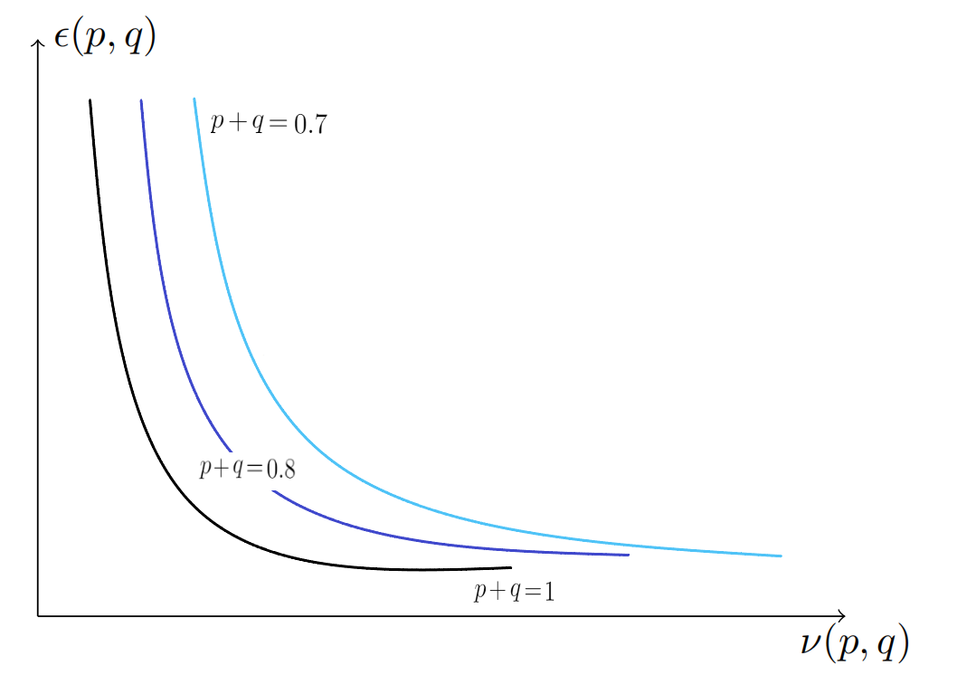
Figure 2: The trade-off in Shafer’s semantics

The trade-off between the privacy loss $\epsilon^{S}(p,q)$ and the accuracy $\nu^{S}(p,q)$ can be illustrated in the following Figure 1. The figure shows clearly the impact of “don’t know" with probability $1-p-q$ on the trade-off between $\epsilon^{S}(p,q)$ and $\nu^{S}(p,q)$. When $1-p-q=0$ or $p+q=1$, the black curve for the trade-off between $\epsilon^{S}(p,q)$ and $\nu^{S}(p,q)$ is exactly for Warner’s randomized response mechanism. If $p+q=c$ where $c$ is a constant, the trade-off curve is similar to that for Warner’s mechanism. Moreover, when the constant $c$ gets smaller or the probability of “don’t know" gets larger, the curve moves further away from that for Warner’s model. Figure 2 tells us that Warner’s model is optimal among those generalized $Q_{2\times 3}$-mechanisms. Next we explore the effect of the sample size on the accuracy of the estimation. We set the sample size to be 10, 100, 500, 1000 and fix $q_{3}=0.1$. From the experimental results (Figure 3), we can see that when the privacy loss is relatively large, different sample sizes can achieve similar estimations. However, when the privacy budget is relatively small, with the increase of the sample size, the estimation variance gets smaller and smaller.

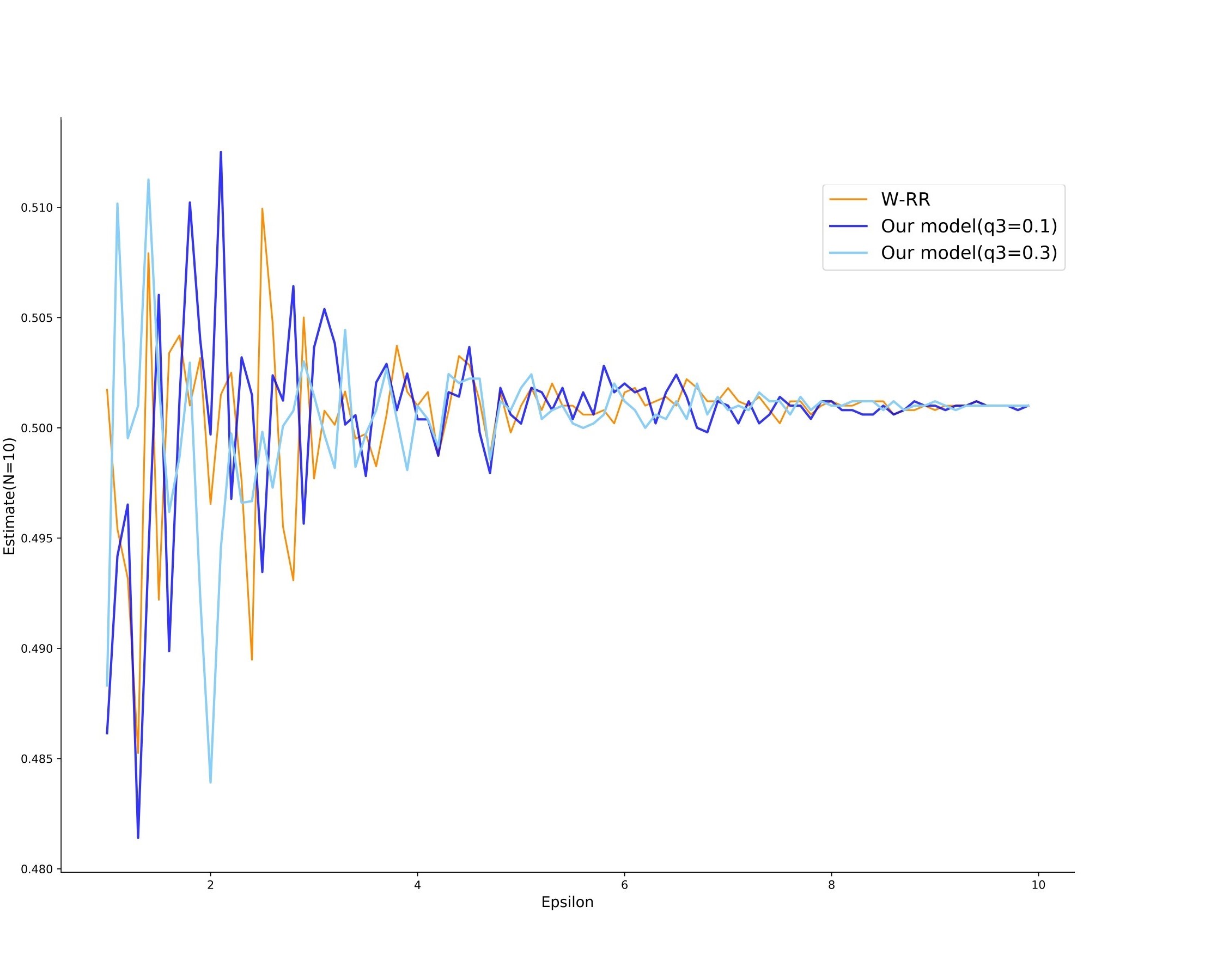
(a) N=10

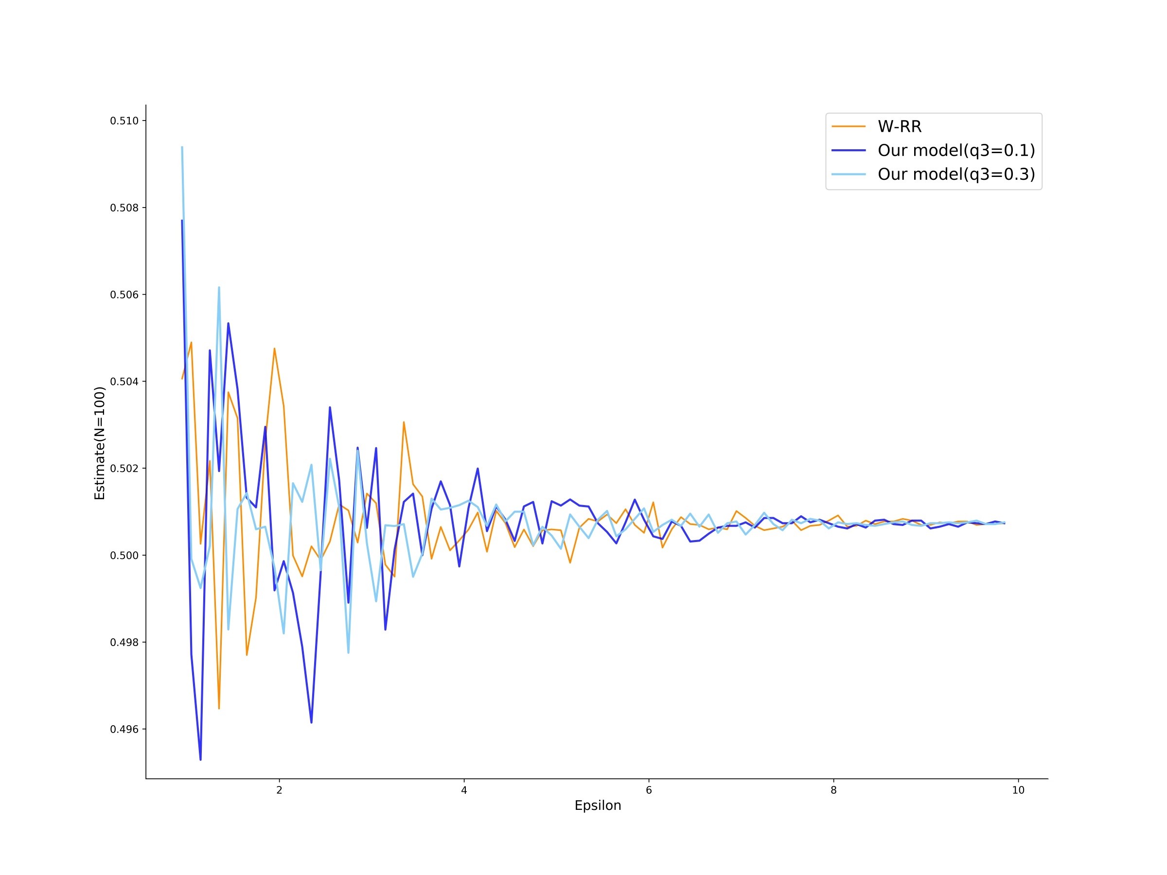
(b) N=100

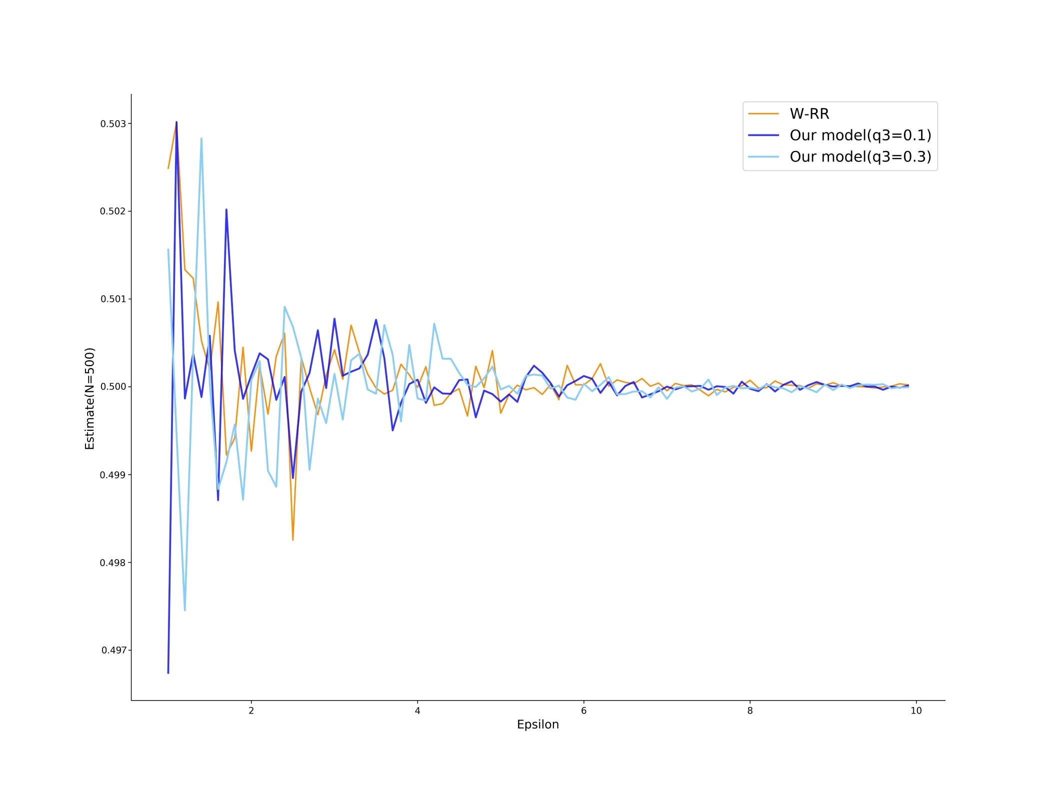
(c) N=500

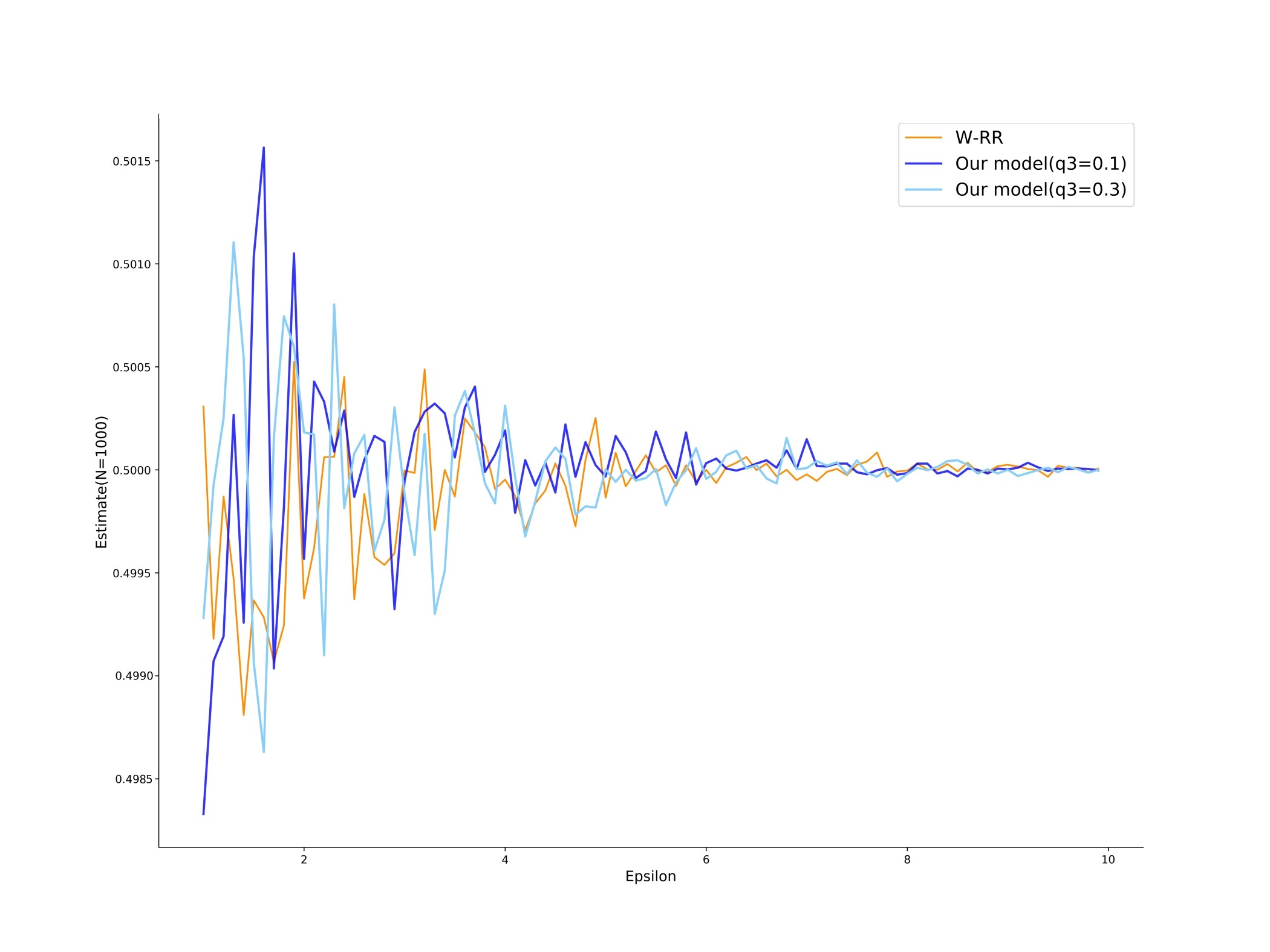
(d) N=1000

Figure 3: Impact of sample sizes on the estimation accuracy

3.2 LDP according to Walley

For an evidential privacy mechanism $Q$, let $r_{Q}^{W}=max_{pr_{x}\in\mathcal{P}_{bel^{Q}_{x}},pr_{x^{\prime}}\in\mathcal{P}_{bel^{Q}_{x^{\prime}}}}\frac{pr_{x}(E)}{pr_{x^{\prime}}(E)}$. And the logarithm $\epsilon_{Q}^{W}=ln(r_{Q}^{W})$ quantifies the privacy loss of the privacy mechanism $Q$ in Walley’s semantics of imprecise probabilities. There is another definition of LDP for belief functions in the setting of imprecise probabilities:

Definition 3.13

For any $\epsilon>0$, $Q$ is called $\epsilon$-locally differential private according to Walley ($\epsilon$-$WLDP$ for short) if, $-\epsilon\leq\epsilon_{Q}^{W}\leq\epsilon$. And $\epsilon^{Q}_{W}$ is called the privacy loss of $Q$ according to Walley and $\epsilon$ is a privacy budget. $\lhd$

In other words, the privacy loss for $\epsilon$-$WLDP$ is defined by consistent probability functions in the worst case. So, $\epsilon$-$WLDP$ fits well with the worst-case analysis behind the philosophy of differential privacy and also with the conservative principle of least commitment in the theory of belief functions [8]. Lemma 3.2 and the following Lemma 3.14 provide a simple mathematical characterization of SLDP and WLDP, where we can see clearly the main difference between Definitions 3.1 and 3.13.

Lemma 3.14

(Alternative formulations) If privacy mechanism $Q$ is $\epsilon$-$WLDP$, then, for all $x,x^{\prime}\in X$ and $E\subseteq Y$: $e^{-\epsilon}\leq\frac{pl_{x}(E)}{bel_{x^{\prime}}(E)}\leq e^{\epsilon}$.

Lemma 3.15

(Composition) Let $Q_{1}$ be an $\epsilon_{1}$-WLDP evidential privacy mechanism from $X$ to $Y_{1}$ and $Q_{2}$ be an $\epsilon_{2}$-WLDP evidential privacy mechanisms from $X$ to $Y_{2}$. Then their combination $Q_{1,2}$ defined by $Q_{1,2}(x)=(Q_{1}(x),Q_{2}(x))$ is $\epsilon_{1}+\epsilon_{2}$-WLDP.

Lemma 3.16

(Post-processing) Let $Q$ be an $\epsilon$-WLDP mechanism from $X$ to $Y$ and $f$ is a data-independent randomized algorithm from $Y$ to another finite alphabet set $Z$. Then $f\circ Q$ is an $\epsilon$-WLDP mechanism from $X$ to $Z$.

For the hypothesis testing problem, recall that $Q$ denotes an evidential privacy mechanism and $\varphi:Y\rightarrow[0,1]$ is a rejection rule. In order to translate $\epsilon$-WLDP into the trade-off between type I and II errors, we have to divide them into two different types of errors: one is pessimistic and the other optimistic. For the rejection rule $\varphi$, the pessimistic type I and II are defined as $\alpha^{pe}_{\varphi}=\text{sup}_{pr\in\mathcal{P}_{bel_{x}^{Q}}}\mathbb{E}_{pr}(\varphi)$ and $\beta^{pe}_{\varphi}=\text{sup}_{pr\in\mathcal{P}_{bel_{x^{\prime}}^{Q}}}\mathbb{E}_{pr}(1-\varphi)$, respectively. They are actually the same as those errors in $\epsilon$-$SLDP$. Also we define the optimistic type I and II errors as $\alpha^{op}_{\varphi}:=\text{inf}_{pr\in\mathcal{P}_{bel_{x}^{Q}}}\mathbb{E}_{pr}(\varphi)$ and $\beta^{op}_{\varphi}:=\text{inf}_{pr\in\mathcal{P}_{bel_{x^{\prime}}^{Q}}}\mathbb{E}_{pr}(1-\varphi)$, respectively.

Definition 3.17

For the above pessimistic errors, the following function is called the pessimistic trade-off function: $T^{pe}(Q(x),Q(x^{\prime}))(\alpha):=inf\{\beta^{pe}_{\varphi}:\alpha^{pe}_{\varphi}\leq\alpha\}$. For the above optimistic errors, the following function is called the optimistic trade-off function: $T^{op}(Q(x),Q(x^{\prime}))(\alpha):=sup\{\beta^{op}_{\varphi}:\alpha^{op}_{\varphi}\leq\alpha\}$. $\lhd$

The following theorem is another generalization of the well-known result (Theorem 2.4 in [36]) for standard differential privacy.

Theorem 3.18

For any evidential privacy mechanism $Q$, the following two statements are equivalent:

1. $Q$ is $\epsilon$-WLDP;

2. For any $\alpha\in[0,1]$, $T^{pe}(Q(x),Q(x^{\prime}))(\alpha)\geq f^{pe}_{\epsilon}(\alpha)$ and $T^{op}(Q(x),Q(x^{\prime}))(\alpha)\leq f^{op}_{\epsilon}(\alpha)$ where $f^{pe}_{\epsilon}(\alpha)=max\{1-\alpha e^{\epsilon},0,e^{-\epsilon}(1-\alpha)\}$ and $f^{op}_{\epsilon}(\alpha)=min\{1-\alpha e^{-\epsilon},e^{\epsilon}(1-\alpha)\}$.

For the composition, the adversary needs to distinguish between $Q(x)\times Q(x)$ and $Q(x^{\prime})\times Q(x^{\prime})$. Similarly, we can define pessimistic and optimistic type I and II errors: $\alpha^{2,pe}_{\varphi},\beta^{2,pe}_{\varphi},\alpha^{2,op}_{\varphi}$ and $\beta^{2,op}_{\varphi}$. Moreover, for the hypothesis testing problem for the composition, we define the pessimistic and optimistic trade-off functions similarly: $T^{pe}_{2}(Q(x)\times Q(x),Q(x^{\prime})\times Q(x^{\prime}))(\alpha):=inf\{\beta^{2,pe}_{\varphi}:\alpha^{2,pe}_{\varphi}\leq\alpha\}$, and $T^{op}_{2}(Q(x)\times Q(x),Q(x^{\prime})\times Q(x^{\prime}))(\alpha):=sup\{\beta^{2,op}_{\varphi}:\alpha^{2,op}_{\varphi}\leq\alpha\}$.

Corollary 3.19

For any $\alpha\in[0,1]$, $T_{2}^{pe}(Q(x)\times Q(x),Q(x^{\prime})\times Q(x^{\prime}))(\alpha)\geq f^{2,pe}_{\epsilon}(\alpha)$ and $T_{2}^{op}(Q(x)\times Q(x),Q(x^{\prime})\times Q(x^{\prime}))(\alpha)\leq f^{2,op}_{\epsilon}(\alpha)$ where $f^{2,pe}_{\epsilon}(\alpha)=max\{1-\alpha e^{2\epsilon},-\alpha+\frac{2}{e^{\epsilon}+1},e^{-2\epsilon}(1-\alpha)\}$ and $f^{2,op}_{\epsilon}(\alpha)=min\{1-\alpha e^{-2\epsilon},e^{2\epsilon}(1-\alpha),-\alpha+\frac{3-e^{-2\epsilon}}{e^{\epsilon}+1}\}$.

Both Theorem 3.18 and Corollary 3.19 can be visualized as follows:

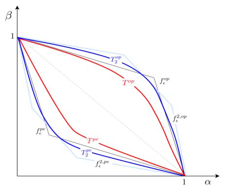
Figure 4: The trade-off between type I and II errors for WLDP

For simplicity, we consider the above evidential privacy matrix

$$Q_{2\times 3}=\left(\begin{array}[]{ccc}p&q&1-p-q\\ q&p&1-p-q\end{array}\right).$$

In Definition 3.1, $1-p-q$ quantifies the conditional probability of the third response “I don’t know". Similarly, in Definition 3.13, $p$ and $q$ are the probabilities of telling truthfully and of lying respectively. However, $1-p-q$ measures the probability of unknown response strategy or possible noncompliance. Unlike SLDP, there are only two responses “Yes" and “No" for response mechanism according to WLDP and “I don’t know" is not an option. In order to obtain a Warner-style randomized response $2\times 2$ matrix, we redistribute the mass $1-p-q$ on the unknown part to those masses on “Yes" and “No" and get the following matrix:

$$Q_{\lambda}=\left(\begin{array}[]{ccc}p+\lambda(1-p-q)&q+(1-\lambda)(1-p-q)\\ q+(1-\lambda)(1-p-q)&p+\lambda(1-p-q)\end{array}\right)$$

When $\lambda=1$, the associated privacy loss is the largest and is the same as according to Definition 3.13. The respondent is most conservative and make the worst-case analysis. On the other hand, when $\lambda=0$, the associated privacy loss is the smallest. In this case, the respondent is the most optimistic and assumes the best possibility. Similarly, we can obtain the maximum likelihood estimation $\hat{\pi}=\frac{\frac{n_{1}}{n}-(1-\lambda)(1-p-q)-q}{p-q+(2\lambda-)(1-p-q)}$, and show that $\hat{\pi}$ is an unbiased estimate of $\pi$. From Theorem 3.10, we know that, when $\lambda=0$, the variance $Var(\hat{\pi})(=\frac{-(\pi-1/2)^{2}+\frac{1}{4(2p-1)^{2}}}{n})$ is the largest and is defined as the estimation accuracy of the privacy matrix $Q_{2\times 3}$ according to Walley.

According to Shafer’s semantics, the privacy loss for the mechanism $Q_{2\times 3}$ is defined as $\epsilon^{S}(p,q)=ln(\frac{p}{q})$ and its accuracy is $\nu^{S}(p,q)=Var(\hat{\pi}|N_{1}+N_{2}\neq 0)=\frac{-(\pi-\frac{1}{2})^{2}+\frac{(p-q)^{2}}{4(p+q)^{2}}}{(n+1)(p+q)-1}$ (Thm. (3.10)). In contrast, according to Walley’s semantics, the privacy loss for $Q_{2\times 3}$ is defined as $ln(\frac{1-q}{q})$, which is denoted as $\epsilon^{W}(p,q)$ and is equal to the privacy loss of the associated matrix $Q_{1}$ in Warner’s model. Moreover its accuracy is $\frac{-(\pi-\frac{1}{2})^{2}+\frac{1}{4(2p-1)^{2}}}{n}$, which is denoted as $\nu^{W}(p,q)$ and is exactly the accuracy for the matrix $Q_{0}$ in Warner’s model. In other words, both $\epsilon^{W}(p,q)$ and $\nu^{W}(p,q)$ are obtained according to the worst-case analysis from the perspectives of the respondent and adversary respectively. Similarly, we may obtain $\epsilon^{O}(p,q)$ and $\nu^{O}(p,q)$, the optimal privacy loss and estimation error among all possible privacy mechanisms $Q_{\lambda}$. The following Figure 5 illustrates the relationships among the three trade-offs between privacy and accuracy: $(\epsilon^{S}(p,q),\nu^{S}(p,q)),(\epsilon^{W}(p,q),\nu^{W}(p,q))$ and $(\epsilon^{O}(p,q),\nu^{O}(p,q))$. The rectangle shown in the figure consists of exactly the trade-offs between privacy and accuracy for all possible $Q_{\lambda}$ with $(\epsilon^{W}(p,q),\nu^{W}(p,q))$ as the worst and $(\epsilon^{O}(p,q),\nu^{O}(p,q))$ as the best.

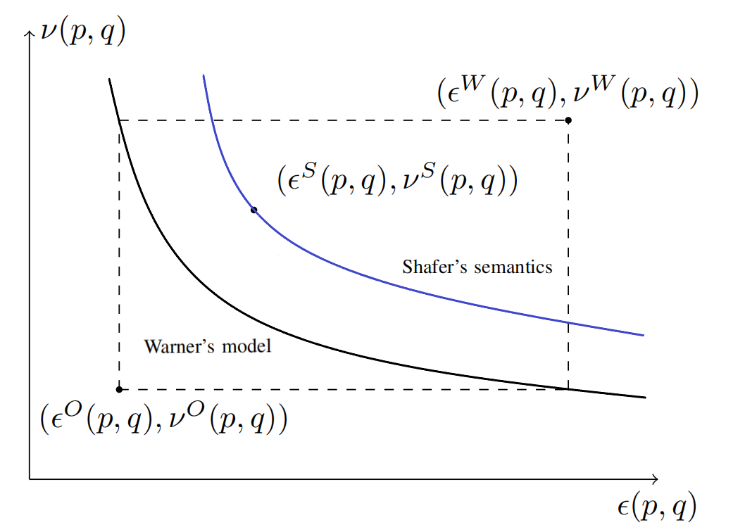
Figure 5: Comparison of trade-offs in the two semantics

Corollary 3.20

$\epsilon^{W}(p,q)$ is decreasing with respect to $q$ and $\nu^{W}(p,q)$ is decreasing with respect to $p$.

According to the corollary, we may compare two privacy mechanisms $Q_{2\times 3}(p,q)$ and $Q_{2\times 3}(p^{\prime},q^{\prime})$. If $p\geq p^{\prime}$ and $q\geq q^{\prime}$, then $\epsilon^{W}(p,q)\leq\epsilon^{W}(p^{\prime},q^{\prime})$ and $\nu^{W}(p,q)\leq\nu^{W}(p^{\prime},q^{\prime})$. In this case, $Q_{2\times 3}(p,q)$ is preferred to $Q_{2\times 3}(p^{\prime},q^{\prime})$. So the trade-off in Walley’s semantics is similar to the minimax estimation for LDP [11].

4 Conclusion

To the best of our knowledge, we are the first to explore differential privacy from a different uncertainty perspective than probability theory. The fact that differential privacy is closely related to statistical analysis [13] may explain why there are few research about DP in other uncertainty theories which don’t support a practical statistical analysis. But belief functions are deeply rooted in fiducial inference, an important school in statistics [6, 31, 26, 25]. It is desirable to develop a belief-function theory of differential privacy. The LDP implicitly requires some assumptions about the adversary’s view of belief functions in privacy mechanism. There are many semantics for belief functions. In this paper, we choose Shafer’s semantics as randomly encoded messages [32] and Walley’s interpretation as imprecise-probabilities [33]. Our work in LDP is motivated by the nonresponse and noncompliance issue in randomized response technique in [35, 15] and discrete distribution estimation problem in [20, 19, 34, 17] where the size of the input alphabet is no less than that of the output alphabet. However, since the number of messages (or the size of the powerset of the output set) is usually larger than that of the input set in our LDP mechanisms, MLE is usually different from empirical estimation in this case and their techniques don’t apply here. Moreover, there is a rich literature to address nonresponse in survey research [24] but most of them regard the issue as a missing-data problem and few of them consider the privacy problem. There seems no obvious LDP definitions for coarsening at random because the outputs of coarsening mechanisms at different inputs are different and hence the adversary can easily distinguish these two inputs. It may be interesting to explore the LDPs for contamination models. There are 2 other possible definitions of SLDP in terms of belief functions and plausibility functions: $e^{-\epsilon}\leq\frac{bel_{x}^{Q}(E)}{bel_{x^{\prime}}^{Q}(E)}\leq e^{\epsilon}$ and $e^{-\epsilon}\leq\frac{pl_{x}^{Q}(E)}{pl_{x^{\prime}}^{Q}(E)}\leq e^{\epsilon}$. Lemma 3.2 and the remarks afterwards actually show their relationships. In future versions, we will elaborate these two different definitions and their relations with Definition 3.1.

In this paper we show a binary composition theorem for each definition (Corollaries 3.6 and 3.19). We believe that, for our two definitions SLDP and WLDP, the composition of the hypothesis-testing trade-off functions [21, 2] converges to some (most probably random-set variant) form of Gaussian DP [9] according to some central limit theorem (Chapter 3 in [27]). In this paper, we took the first step in this direction and showed the effect of the composition of hypothesis-testing trade-off functions(Corollaries 1 and 4). Moreover, we would like to investigate LDP for belief functions from the perspective of respondents (as in [37]) and conduct a series of rigorous surveys to show that our new generalized Warner’s mechanism including “don’t know" as an option can indeed increase user’s willingness to participate.

Supplementary-Materials

Proof of Lemma 3.2: These two propositions follow directly from the inequality (1) and the facts that $bel_{x}(E)=\sum_{E^{\prime}\subseteq E}m(E^{\prime})$ and $pl_{x}(E)=\sum_{E^{\prime}\cap E\neq\emptyset}m(E^{\prime})$.

Proof of Lemma 3.3: The composition follows from the fact that $\frac{m^{Q_{12}}_{x}(E_{1},E_{2})}{m^{Q_{12}}_{x^{\prime}}(E_{1},E_{2})}=\frac{m^{Q_{1}}_{x}(E_{1})}{m^{Q_{1}}_{x^{\prime}}(E_{1})}\frac{m^{Q_{2}}_{x}(E_{2})}{m^{Q_{2}}_{x^{\prime}}(E_{2})}$.

Proof of Lemma 3.4: The proof for $\epsilon$-SLDP algorithm is similar to that of the post-processing property for probabilistic privacy mechanisms (Proposition 2.1 in [13]). We prove the proposition only for a deterministic function $f:Y\rightarrow Z$. For any $x,x^{\prime}\in X$, $m_{x}^{f\circ Q}(E)=m_{x}^{Q}(f^{-1}(E))\leq e^{\epsilon}m_{x^{\prime}}^{Q}(f^{-1}(E))$.

Proof of Theorem 3.5: Let’s assume that the rejection region for the hypothesis testing problem is $R$. Let $Q$ be $\epsilon$-SLDP.

1. Assume that $pl_{x}^{Q}(R)\leq\alpha$. It follows that, for any $E\subseteq Y$, $-\epsilon\leq\frac{m_{x}^{Q}}{m^{Q}_{x^{\prime}}}\leq e^{\epsilon}$. We have that $e^{\epsilon}bel_{x^{\prime}}^{Q}(R^{c})\geq bel_{x}^{Q}(R^{c})\geq 1-\alpha$. So $bel_{x^{\prime}}^{Q}(R^{c})\geq e^{-\epsilon}(1-\alpha)$. So, $pl_{x^{\prime}}(R)\leq 1-e^{-\epsilon}(1-\alpha)$. Moreover, $pl_{x^{\prime}}^{Q}(R)\leq e^{\epsilon}pl_{x}^{Q}(R)=e^{\epsilon}\alpha$. By putting these together, we obtain that $pl_{x^{\prime}}^{Q}(R)\leq min\{e^{\epsilon}\alpha,1-e^{-\epsilon}(1-\alpha)\}$. This implies that the type 2 error $\beta_{\varphi}\geq max\{1-e^{\epsilon}\alpha,e^{-\epsilon}(1-\alpha)\}$.

2. If we asssume that, $bel_{x}^{Q}(R)\leq\alpha^{\prime}$, then $pl_{x}^{Q}(R^{c})\leq 1-\alpha^{\prime}$. Since $e^{-\epsilon}pl_{x^{\prime}}^{Q}(R^{c})\leq pl_{x}^{Q}(R^{c})$, $pl_{x^{\prime}}^{Q}(R^{c})\leq e^{\epsilon}(1-\alpha^{\prime})$. It follows that $bel_{x^{\prime}}^{Q}(R)\geq 1-e^{\epsilon}(1-\alpha^{\prime})$. Moreover, $bel_{x^{\prime}}^{Q}(R)\geq e^{-\epsilon}bel_{x}^{Q}(R)\geq\alpha^{\prime}e^{-\epsilon}$. By puting these together, we have that $bel_{x^{\prime}}^{Q}(R)\geq max\{\alpha^{\prime}e^{-\epsilon},1-e^{\epsilon}(1-\alpha^{\prime})\}$.

In other words, if type I error $\alpha_{\varphi}\in[l,L]$, then type II error $\beta_{\varphi}\in[u(L),U(l)]$ where $u(\alpha)=max\{e^{-\epsilon}(1-\alpha),1-\alpha e^{\epsilon}\}$ and $U(\alpha)=min\{e^{\epsilon}(1-\alpha),1-\alpha e^{-\epsilon}\}$. Since the reasonings above are birectional, the direction from (2) to (1) can be shown similarly.

Proof of Corollary 3.6: Let $Q_{2\times 3}$ denote a known row-stochastic matrix as follows:

$$Q_{2\times 3}=\left(\begin{array}[]{ccc}p&q&1-p-q\\ q&p&1-p-q\end{array}\right)$$

where $p,q\in[0,1]$. $Q_{2\times 3}$ may be regarded as a generalized Warner’s randomized response mechanism where a respondent answers truthfully with probability $p$, tells a lie with $q$ and don’t respond or respond “I don’t know" with probability $1-p-q$. Let $Q_{x}$ denotes the first row of $Q$ and $Q_{x^{\prime}}$ the second row. Now we consider the hypothesis testing problem by distinguishing between $Q_{x}\times Q_{x}$ and $Q_{x^{\prime}}\times Q_{x^{\prime}}$. Let $m^{\otimes 2}_{x}$ and $m^{\otimes 2}_{x^{\prime}}$ denote their corresponding mass functions. Their output set is $\{0,1,2\}$.

$m^{\otimes 2}_{x}$	$\{0\}$	$\{1\}$	$\{2\}$	$\{0,1\}$	$\{1,2\}$	$\{0,1,2\}$
	$p^{2}$	$2pq$	$q^{2}$	$2p(1-p-q)$	$2q(1-p-q)$	$(1-p-q)^{2}$

And

$m^{\otimes 2}_{x^{\prime}}$	$\{0\}$	$\{1\}$	$\{2\}$	$\{0,1\}$	$\{1,2\}$	$\{0,1,2\}$
	$q^{2}$	$2pq$	$p^{2}$	$2q(1-p-q)$	$2p(1-p-q)$	$(1-p-q)^{2}$

Since $Q$ is $\epsilon$-SLDP, we have

$e^{-\epsilon}\leq\frac{1-q}{q},\frac{1-p}{p}\leq e^{\epsilon}$.

Let $R$ be a rejection region and assume that $\alpha^{\prime}\leq pl_{x}^{Q\times Q}(R)\leq\alpha$. If $(1-p)^{2}\leq\alpha$, then $p^{2}\leq e^{2\epsilon}\alpha$. Since $e^{\epsilon}\geq 1$, $p\geq\frac{2-e^{\epsilon}}{e^{\epsilon}+1}$. It follows that $(2-p)p\leq e^{2\epsilon}(1-p^{2})$ and $1-(1-p)^{2}\leq e^{2\epsilon}(1-p^{2})$. So we have that $p^{2}\leq 1-e^{-2\epsilon}[1-(1-p)^{2}]$. Since $1-e^{-2\epsilon}[1-(1-p)^{2}]\leq 1-(1-x)e^{-2\epsilon}$. so we havs shown that if the type 1 error is $\leq\alpha$, then the type 2 error is at least $u^{2}(\alpha):=max\{e^{-2\epsilon}(1-\alpha),-\alpha+\frac{2}{e^{\epsilon}+1},1-\alpha e^{2\epsilon}\}$. For the other part, we can show similarly: if the type 1 error is at most $\alpha$, then the type 2 error is at least $U^{2}(\alpha):=min\{e^{2\epsilon}(1-\alpha),1-\alpha e^{-2\epsilon},-\alpha+\frac{3-e^{-2\epsilon}}{e^{\epsilon}+1}\}$.

Lemma 4.1

$\mathbb{E}[\frac{N_{1}}{N_{1}+N_{2}}]=\frac{q_{1}}{q_{1}+q_{2}}(1-q_{3}^{n})$, and $\mathbb{E}[\frac{N_{2}}{N_{1}+N_{2}}]=\frac{q_{2}}{q_{1}+q_{2}}(1-q_{3}^{n})$.

Proof of Lemma 0.1: We only prove the first part and the proof of the second is similar.

$$\mathbb{E}[\frac{N_{1}}{N_{1}+N_{2}}] =\sum_{n_{1}+n_{2}+n_{3}=n,n_{1}+n_{2}\neq 0}\frac{n_{1}}{n_{1}+n_{2}}\binom{n}{n_{3}}\binom{n_{1}+n_{2}}{n_{1}}q_{1}^{n_{1}}q_{2}^{n_{2}}q_{3}^{n_{3}}$$

$$=\sum_{n_{1}+n_{2}+n_{3}=n,n_{1}\neq 0}\frac{n_{1}}{n_{1}+n_{2}}\binom{n}{n_{3}}\binom{n_{1}+n_{2}}{n_{1}}q_{1}^{n_{1}}q_{2}^{n_{2}}q_{3}^{n_{3}}$$

$$=q_{1}\sum_{n_{1}+n_{2}+n_{3}=n,n_{1}\neq 0}\binom{n}{n_{3}}\binom{n_{1}+n_{2}-1}{n_{1}-1}q_{1}^{n_{1}-1}q_{2}^{n_{2}}q_{3}^{n_{3}}$$

$$=q_{1}\sum_{1\leq n_{3}\leq n-1}\binom{n}{n_{3}}q_{3}^{n_{3}}[\sum_{n_{1}+n_{2}=n-n_{3},n_{1}\neq 0}\binom{n_{1}+n_{2}-1}{n_{1}-1}q_{1}^{n_{1}-1}q_{2}^{n_{2}}]$$

$$=q_{1}\sum_{1\leq n_{3}\leq n-1}\binom{n}{n_{3}}q_{3}^{n_{3}}(q_{1}+q_{2})^{n_{1}+n_{2}-1}$$

$$=\frac{q_{1}}{q_{1}+q_{2}}[(q_{1}+q_{2}+q_{3})^{n}-q_{3}^{n}]$$

$$=\frac{q_{1}}{q_{1}+q_{2}}(1-q_{3}^{n})$$

Proof of Theorem 3.9: The equality $\mathbb{E}[\frac{N_{2}q-N_{1}p}{(N_{1}+N_{2})(q-p)}]=\pi(1-q_{3}^{n})$ follows directly from the above lemma and the formula for MLE.

The proof of Theorem 3.10 is much more involved. It needs the following five necessary lemmas which are not stated in the main text. Recall that $n$ is the sample size. Let $A=\sum_{0\leq N_{3}<n}\frac{1}{n-N_{3}}$ ${n}\choose{N_{3}}$$(1-q_{3})^{n-N_{3}}q_{3}^{N_{3}}$ and $f(q_{1},n_{3})=\sum_{n_{1}+n_{2}=n-n_{3},n_{1}\neq 0}n_{1}\binom{n_{1}+n_{2}-1}{n_{1}-1}q_{1}^{n_{1}-1}q_{2}^{n_{2}}$.

Lemma 4.2

$$f(q_{1},n_{3})=\left\{\begin{array}[]{rl}1&\text{ if }n_{3}=n-1,\\ (q_{1}+q_{2})^{n-n_{3}-1}+(n-n_{3}-1)q_{1}(q_{1}+q_{2})^{n-n_{3}-2}&\text{ if }n_{3}\leq n-2.\end{array}\right.$$

Proof.

First we compute the integral of $f(x,n_{3})$.

$$\int_{0}^{x}f(t,n_{3})dt =\sum_{n_{1}+n_{2}=n-n_{3},n_{1}\neq 0}\int_{0}^{x}n_{1}\binom{n_{1}+n_{2}-1}{n_{1}-1}t^{n_{1}-1}q_{2}^{n_{2}}dt$$

$$=\sum_{n_{1}+n_{2}=n-n_{3},n_{1}\neq 0}\binom{n_{1}+n_{2}-1}{n_{1}-1}x^{n_{1}}q_{2}^{n_{2}}$$

$$=x(x+q_{2})^{n-n_{3}-1}$$

So $f(x,n_{3})=(\int_{0}^{x}f(t)dt)^{\prime}=(x+q_{2})^{n-n_{3}-1}+(n-n_{3}-1)x(x+q_{2})^{n-n_{3}-2}$. ∎

Lemma 4.3

$\sum_{0\leq n_{3}\leq n-1}\frac{1}{n-n_{3}}(q_{1}+q_{2})^{n-n_{3}-1}\binom{n}{n_{3}}q_{3}^{n_{3}}=\frac{A}{(q_{1}+q_{2})}$.

Lemma 4.4

$\sum_{0\leq n_{3}\leq n-2}(q_{1}+q_{2})^{n-n_{3}-2}\binom{n}{n_{3}}q_{3}^{n_{3}}=\frac{1-q_{3}^{n}-n(q_{1}+q_{2})q_{3}^{n-1}}{(q_{1}+q_{2})^{2}}$.

Proof.

It follows from the fact that

$$[(q_{1}+q_{2})+q_{3}]^{n} =[\sum_{0\leq n_{3}\leq n-2}(q_{1}+q_{2})^{n-n_{3}-2}\binom{n}{n_{3}}q_{3}^{n_{3}}]+q_{3}^{n}+n(q_{1}+q_{2})q_{3}^{n-1}.$$

∎

Lemma 4.5

$\sum_{0\leq n_{3}\leq n-2}\frac{1}{n-n_{3}}(q_{1}+q_{2})^{n-n_{3}-2}\binom{n}{n_{3}}q_{3}^{n_{3}}=\frac{A-n(q_{1}+q_{2})q_{3}^{n-1}}{(q_{1}+q_{2})^{2}}$.

Proof.

It follows directly from the definition of $A$. ∎

Lemma 4.6

• $\mathbb{E}[(\frac{N_{1}}{N_{1}+N_{2}})^{2}]=\frac{q_{1}q_{2}}{(q_{1}+q_{2})^{2}}A+\frac{q_{1}^{2}}{(q_{1}+q_{2})^{2}}(1-q_{3}^{n})$

• $\mathbb{E}[(\frac{N_{2}}{N_{1}+N_{2}})^{2}]=\frac{q_{1}q_{2}}{(q_{1}+q_{2})^{2}}A+\frac{q_{2}^{2}}{(q_{1}+q_{2})^{2}}(1-q_{3}^{n})$.

Proof.

We only show the first part and the proof of the second is similar.

$$\mathbb{E}[(\frac{N_{1}}{N_{1}+N_{2}})^{2}]= \sum_{n_{1}+n_{2}+n_{3}=n,n_{1}\neq 0}(\frac{n_{1}}{n_{1}+n_{2}})^{2}\binom{n_{1}+n_{2}}{n_{1}}\binom{n}{n_{3}}q_{1}^{n_{1}}q_{2}^{n_{2}}q_{3}^{n_{3}}$$

$$= q_{1}\sum_{n_{1}+n_{2}+n_{3}=n,n_{1}\neq 0}\frac{1}{n-n_{3}}n_{1}\binom{n_{1}+n_{2}-1}{n_{1}-1}\binom{n}{n_{3}}q_{1}^{n_{1}-1}q_{2}^{n_{2}}q_{3}^{n_{3}}$$

$$= q_{1}\sum_{0\leq n_{3}\leq n-1}\frac{1}{n-n_{3}}[\sum_{n_{1}+n_{2}=n-n_{3},n_{1}\neq 0}n_{1}\binom{n_{1}+n_{2}-1}{n_{1}-1}q_{1}^{n_{1}-1}q_{2}^{n_{2}}]\binom{n}{n_{3}}q_{3}^{n_{3}}$$

$$= q_{1}[\sum_{0\leq n_{3}\leq n-1}\frac{1}{n-n_{3}}(q_{1}+q_{2})^{n-n_{3}-1}\binom{n}{n_{3}}q_{3}^{n_{3}}+q_{1}\sum_{0\leq n_{3}\leq n-2}(q_{1}+q_{2})^{n-n_{3}-2}\binom{n}{n_{3}}q_{3}^{n_{3}}-$$

$$q_{1}\sum_{0\leq n_{3}\leq n-2}\frac{1}{n-n_{3}}(q_{1}+q_{2})^{n-n_{3}-2}\binom{n}{n_{3}}q_{3}^{n_{3}}]\text{ (Lemma 0.2) }$$

$$= q_{1}[\frac{A}{(q_{1}+q_{2})}+q_{1}\frac{1-q_{3}^{n}-n(q_{1}+q_{2})q_{3}^{n-1}}{(q_{1}+q_{2})^{2}}-q_{1}\frac{A-n(q_{1}+q_{2})q_{3}^{n-1}}{(q_{1}+q_{2})^{2}}]\text{ (Lemmas 0.3, 0.4,0.5) }$$

$$= \frac{q_{1}q_{2}}{(q_{1}+q_{2})^{2}}A+\frac{q_{1}^{2}}{(q_{1}+q_{2})^{2}}(1-q_{3}^{n})$$

∎

Proof of Theorem 3:

$$Var[\hat{\pi}|N_{1}+N_{2}\neq 0] =Var[\frac{N_{2}q-N_{1}p}{(N_{1}+N_{2})(q-p)}|N_{1}+N_{2}\neq 0]$$

$$=Var[\frac{N_{2}q+N_{2}p-(N_{1}+N_{2})p}{(N_{1}+N_{2})(q-p)}|N_{1}+N_{2}\neq 0]$$

$$=Var[\frac{N_{2}}{N_{1}+N_{2}}\frac{p+q}{q-p}-\frac{p}{q-p}|N_{1}+N_{2}\neq 0]$$

$$=\frac{(p+q)^{2}}{(q-p)^{2}}Var[\frac{N_{2}}{N_{1}+N_{2}}|N_{1}+N_{2}\neq 0]$$

$$=\frac{(p+q)^{2}}{(q-p)^{2}}[E[(\frac{N_{2}}{N_{1}+N_{2}})^{2}|N_{1}+N_{2}\neq 0]-E[\frac{N_{2}}{N_{1}+N_{2}}|N_{1}+N_{2}\neq 0]^{2}]$$

$$=\frac{(p+q)^{2}}{(q-p)^{2}}[\frac{q_{1}q_{2}}{(q_{1}+q_{2})^{2}}A+\frac{q_{2}^{2}}{(q_{1}+q_{2})^{2}}-\frac{q_{2}^{2}}{(q_{1}+q_{2})^{2}}]\text{ (Lemma 0.6) }$$

$$=\frac{1}{(q-p)^{2}}q_{1}q_{2}A$$

$$=\frac{1}{(q-p)^{2}}[\pi p+(1-\pi)q][\pi q+(1-\pi)p]A$$

Proof of Corollary 3.11: $f^{\prime}(q)=\frac{(n+1)(q+3p)+(\pi-1/2)(p+q)}{(p-q)^{3}(n+1)}>0$.

Proof of Corollary 3.12: When $p+q$ is a constant, the optimaility of $Q_{GWRR}$ follows from the same arguments for $G_{WRR}$ (Example 1) in [35] and [16].

Proof of Lemma 3.14: $\mathcal{P}_{bel_{x}}=\{pr:pr\text{ is a probability distribution and }pr(A)\geq bel_{x}(A)\text{ for all }A\}$ and $\mathcal{P}_{bel_{x^{\prime}}}=\{pr:pr\text{ is a probability distribution and }pr(A)\geq bel_{x^{\prime}}(A)\text{ for all }A\}$. For a given $E\subseteq Y$, by using specialization matrices in [23], we can always find a $pr_{x}\in\mathcal{P}_{bel_{x}}$ such that $pr_{x}(E)=pl_{x}(E)$ and a $pr_{x^{\prime}}$ such that $pr_{x^{\prime}}(E)=bel_{x^{\prime}}(E)$. And Lemma 5 follows directly.

Proof of Lemma 3.15: The proof is similar to that for Lemma 2.

Proof of Lemma 3.16: According to the well-known weak von-Neumann-Birkhoff Lemma, we only need to prove the proposition only for a deterministic function $f:Y\rightarrow Z$. The proof for $\epsilon$-SLDP algorithm is similar to that of the post-processing property for probabilistic privacy mechanisms. For $\epsilon$-WLDP, consider the two probability functions $p_{x}$ and $p_{x^{\prime}}$ such that

$$r^{Q}_{W}=\frac{p_{x}(E)}{p_{x^{\prime}}(E)}$$ (3)

for some $E$. Then

$$r^{f\circ Q}_{W} =max_{x,x^{\prime}\in X,E\subseteq Z}\frac{p_{x}f^{-1}(E)}{p_{x^{\prime}}f^{-1}(E)}$$

$$\leq max_{x,x^{\prime}\in X,E\subseteq Z}\frac{p_{x}(E)}{p_{x^{\prime}}(E)}$$

$$\leq r^{Q}_{W}.$$

Proof of Theorem 3.18 Let $R$ be a rejection region. Since $Q$ is $\epsilon$-WLDP, the following inequalities hold:

$$e^{-\epsilon} \leq\frac{pl_{x^{\prime}}^{Q}(R)}{bel_{x}^{Q}(R)},\frac{pl_{x}^{Q}(R)}{bel_{x^{\prime}}^{Q}(R)}\leq e^{\epsilon}$$ (4)

$$e^{-\epsilon} \leq\frac{pl_{x^{\prime}}^{Q}(R^{c})}{bel_{x}^{Q}(R^{c})},\frac{pl_{x}^{Q}(R^{c})}{bel_{x^{\prime}}^{Q}(R^{c})}\leq e^{\epsilon}$$ (5)

1. Assume that $pl_{x}^{Q}(R)\leq\alpha$. It follows that $e^{-\epsilon}bel_{x^{\prime}}^{Q}(R)\leq pl_{x}^{Q}(R)\leq\alpha$. This implies that $bel_{x^{\prime}}^{Q}(R)\leq e^{\epsilon}\alpha$. So $pl_{x^{\prime}}^{Q}(R^{c})\geq 1-e^{\epsilon}\alpha$. Moreover, Since $bel_{x}^{Q}(R^{c})\leq e^{\epsilon}pl_{x^{\prime}}^{Q}(R^{c})$, $1-e^{\epsilon}pl_{x^{\prime}}^{Q}(R^{c})\leq 1-bel_{x}^{Q}(R^{c})=pl_{x}^{Q}(R)\leq\alpha$. So we have that $pl_{x^{\prime}}(R^{c})\geq e^{-\epsilon}(1-x)$. Putting all these togther, we obtain that $T^{pe}(Q(x),Q(x^{\prime}))(\alpha)\geq max\{1-\alpha e^{\epsilon},0,e^{-\epsilon}(1-\alpha)\}$.

2. Assume that $pl_{x}^{Q}(R^{c})\geq\alpha$. Since $pl_{x}^{Q}(R^{c})\leq e^{\epsilon}bel_{x^{\prime}}^{Q}(R^{c})=e^{\epsilon}(1-pl_{x^{\prime}}^{Q}(R))$, $pl_{x^{\prime}}^{Q}(1-\alpha)$. Moreover, $\alpha\leq pl_{x^{\prime}}^{Q}(R^{c})\leq e^{\epsilon}bel_{x}^{Q}(R^{c})=e^{\epsilon}(1-pl_{x}^{Q}(R))$. It follows that $pl_{x^{\prime}}^{Q}(R)\leq 1-e^{-\epsilon}\alpha$. So $T^{op}(Q(x),Q(x^{\prime}))(\alpha)\leq min\{1-\alpha e^{-\epsilon},e^{\epsilon}(1-\alpha)\}$.

The other direction of the equivalence can shown in a similar way. We have finished the proof of Theorem 4.

Proof of Corollary 3.19 The proof is similar to that for Corollary 1. The only things that we need to pay much attention to is the direction of the inequalities.

Proof of Corollary 3.20: From the above analysis, we know that $\epsilon^{W}(p,q)$ is defined as the privacy loss of the following matrix $Q_{1}$ in Warner’s model:

$$Q_{1}=\left(\begin{array}[]{ccc}1-q&q\\ q&1-q\end{array}\right)$$

So $\epsilon^{W}(p,q)=ln(\frac{1-q}{q})$ and it is decreasing with respct to $q$. And $\nu^{W}(p,q)$ is defined as the accuracy of the following matrix $Q_{0}$ in Warner’s model:

$$Q_{0}=\left(\begin{array}[]{ccc}p&1-p\\ 1-p&p\end{array}\right)$$

So $\nu^{W}(p,q)=\frac{-(\pi-1/2)^{2}+\frac{1}{4}(\frac{1}{2p-1})^{2}}{n}$ and it is decreasing with respect to $p$.

References

- [1] Dakshi Agrawal and Charu C Aggarwal. On the design and quantification of privacy preserving data mining algorithms. In Proceedings of the twentieth ACM SIGMOD-SIGACT-SIGART symposium on Principles of database systems, pages 247–255, 2001.
- [2] Borja Balle, Gilles Barthe, Marco Gaboardi, Justin Hsu, and Tetsuya Sato. Hypothesis testing interpretations and Rényi differential privacy. In International Conference on Artificial Intelligence and Statistics, pages 2496–2506. PMLR, 2020.
- [3] Brooke Bullek, Stephanie Garboski, Darakhshan J Mir, and Evan M Peck. Towards understanding differential privacy: When do people trust randomized response technique? In Proceedings of the 2017 CHI Conference on Human Factors in Computing Systems, pages 3833–3837, 2017.
- [4] Rachel Cummings, Gabriel Kaptchuk, and Elissa M Redmiles. " i need a better description": An investigation into user expectations for differential privacy. In Proceedings of the 2021 ACM SIGSAC Conference on Computer and Communications Security, pages 3037–3052, 2021.
- [5] Fabio Cuzzolin. The Geometry of Uncertainty - The Geometry of Imprecise Probabilities. Artificial Intelligence: Foundations, Theory, and Algorithms. Springer, 2021.
- [6] Arthur Dempster. Upper and lower probabilities induced by a multivalued mapping. Annals of Math. Stat., 38:325–339, 1967.
- [7] Arthur P. Dempster. The dempster-shafer calculus for statisticians. Int. J. Approx. Reason., 48(2):365–377, 2008.
- [8] Thierry Denoeux. Likelihood-based belief function: Justification and some extensions to low-quality data. Int. J. Approx. Reasoning, 55(7):1535–1547, 2014.
- [9] Jinshuo Dong, Aaron. Roth, and Wenjie. Su. Gaussian differential privacy. Journal of the Royal Statistical Society: Series B (JRSSB), to appear, 2021.
- [10] John Duchi, Michael I. Jordan, and Martin J. Wainwright. Local privacy and statistical minimax rates. In FOCS 2013, 26-29 October, 2013, Berkeley, CA, USA, pages 429–438. IEEE Computer Society, 2013.
- [11] John C. Duchi, Michael I. Jordan, and Martin J. Wainwright. Minimax optimal procedures for locally private estimation. Journal of American Statistical Association, 113(521):182–215, 2018.
- [12] Cynthia Dwork, Frank McSherry, Kobbi Nissim, and Adam D. Smith. Calibrating noise to sensitivity in private data analysis. In Shai Halevi and Tal Rabin, editors, Theory of Cryptography, Third Theory of Cryptography Conference, TCC 2006, New York, NY, USA, March 4-7, 2006, Proceedings, volume 3876 of Lecture Notes in Computer Science, pages 265–284. Springer, 2006.
- [13] Cynthia Dwork and Aaron Roth. The algorithmic foundations of differential privacy. Found. Trends Theor. Comput. Sci., 9(3-4):211–407, 2014.
- [14] Edwin L. Grab and I. Richard Savage. Tables of the expected value of 1/x for positive bernoulli and poisson variables. Journal of the American Statistical Association, 49(256):169–177, 1954.
- [15] Blair Graeme, Kosuke Imai, and Yang-Yang Zhou. Design and analysis of the randomized response technique. Journal of the American Statistical Association, 110(511):1304–1319, 2015.
- [16] Naoise Holohan, Douglas J. Leith, and Oliver Mason. Optimal differentially private mechanisms for randomised response. IEEE Trans. Inf. Forensics Secur., 12(11):2726–2735, 2017.
- [17] Zhengli Huang and Wenliang Du. Optrr: Optimizing randomized response schemes for privacy-preserving data mining. In 2008 IEEE 24th International Conference on Data Engineering, pages 705–714. IEEE, 2008.
- [18] Peter J. Huber and Volker Strassen. Minimax tests and Neyman-Pearson tests for capacities. The Annals of Statistics, 1(2):251–263, 1973.
- [19] Peter Kairouz, Keith Bonawitz, and Daniel Ramage. Discrete distribution estimation under local privacy. In Maria-Florina Balcan and Kilian Q. Weinberger, editors, ICML 2016, New York City, NY, USA, June 19-24, 2016, volume 48, pages 2436–2444. JMLR.org, 2016.
- [20] Peter Kairouz, Sewoong Oh, and Pramod Viswanath. Extremal mechanisms for local differential privacy. J. Mach. Learn. Res., 17:17:1–17:51, 2016.
- [21] Peter Kairouz, Sewoong Oh, and Pramod Viswanath. The composition theorem for differential privacy. IEEE Transactions on Information Theory, 63(6):4037–4049, 2017.
- [22] Shiva Prasad Kasiviswanathan, Homin K. Lee, Kobbi Nissim, Sofya Raskhodnikova, and Adam D. Smith. What can we learn privately? In FOCS 2008, October 25-28, 2008, Philadelphia, PA, USA, pages 531–540. IEEE Computer Society, 2008.
- [23] Frank Klawonn and Philippe Smets. The dynamic of belief in the transferable belief model and specialization-generalization matrices. In UAI ’92, Stanford, CA, USA, July 17-19, 1992, pages 130–137, 1992.
- [24] Roderick.J.A. Little and Donald.B. Rubin. Statistical analysis with missing data. Wiley, 2002.
- [25] Ryan Martin. False confidence, non-additive beliefs, and valid statistical inference. International Journal of Approximate Reasoning, 113:39–73, 2019.
- [26] Ryan Martin and Chuanhai Liu. Inferential models: reasoning with uncertainty, volume 145. CRC Press, 2015.
- [27] Ilya Molchanov. Theory of Random Sets, volume 87 of Probability Theory and Stochastic Modelling. Springer, 2017.
- [28] Jack Murtagh and Salil P. Vadhan. The complexity of computing the optimal composition of differential privacy. Theory Comput., 14(1):1–35, 2018.
- [29] Kopo M Ramokapane, Gaurav Misra, Jose Such, and Sören Preibusch. Truth or dare: Understanding and predicting how users lie and provide untruthful data online. In Proceedings of the 2021 CHI Conference on Human Factors in Computing Systems, pages 1–15, 2021.
- [30] Glenn Shafer. A Mathematical Theory of Evidence. Princeton University Press, Princeton, N.J., 1976.
- [31] Glenn Shafer. Belief function and parametric models (with discussion). J. Roy. Statist. Soc. Ser. B, 23:322–352, 1982.
- [32] Glenn Shafer and Amos Tversky. Languages and designs for probability judgment. Cogn. Sci., 9(3):309–339, 1985.
- [33] Peter Walley. Statistical Reasoning with Imprecise Probabilities. Chapman and Hall, 1990.
- [34] Tianhao Wang, Jeremiah Blocki, Ninghui Li, and Somesh Jha. Locally differentially private protocols for frequency estimation. In Engin Kirda and Thomas Ristenpart, editors, 26th USENIX Security Symposium, USENIX Security 2017, Vancouver, BC, Canada, August 16-18, 2017, pages 729–745. USENIX Association, 2017.
- [35] Stanley Warner. Randomized response: A survey technique for eliminating evasive answer bias. Journal of the American Statistical Association, 60(309):63–69, 1965.
- [36] Larry Wasserman and Shuheng Zhou. A statistical framework for differential privacy. Journal of the American Statistical Association, 105(489):375–389, 2010.
- [37] Aiping Xiong, Tianhao Wang, Ninghui Li, and Somesh Jha. Towards effective differential privacy communication for users’ data sharing decision and comprehension. In 2020 IEEE Symposium on Security and Privacy, SP 2020, San Francisco, CA, USA, May 18-21, 2020, pages 392–410. IEEE, 2020.