Comparison of standard and stabilization free Virtual Elements on anisotropic elliptic problems

Abstract

In this letter we compare the behaviour of standard Virtual Element Methods (VEM) and stabilization free Enlarged Enhancement Virtual Element Methods (E²VEM) with the focus on some elliptic test problems whose solution and diffusivity tensor are characterized by anisotropies. Results show that the possibility to avoid an arbitrary stabilizing part, offered by E²VEM methods, can reduce the magnitude of the error on general polygonal meshes and help convergence.

1 Introduction

In recent years, polytopal methods for the solution of PDEs have received a huge attention from the scientific community. VEM were introduced in [3, 1, 4] as a family of methods that deal with polygonal and polyhedral meshes without building an explicit basis of functions on each element, but rather defining the local discrete spaces and degrees of freedom in such a way that suitable polynomial projections of basis functions are computable. The problem is discretized with bilinear forms that consist of a polynomial part that mimics the operator and an arbitrary stabilizing bilinear form. In [2], error analysis focused on anisotropic elliptic problems shows that the stabilization term adds an isotropic component of the error, independently of the nature of the problem. In [5], a modified version of the method, E²VEM, was proposed, designed to allow the definition of coercive bilinear forms that consist only of a polynomial approximation of the problem operator. In this letter, we apply the two methods to solve some test Laplace problems with anisotropic solutions and diffusivity tensors. For each test, we compare the relative energy errors done by each method.

Let $\Omega\subset\mathbb{R}^{2}$ be a bounded open set with Lipschitz boundary. We look for a solution of Laplace problem with homogeneous Dirichlet boundary conditions, that in variational form reads: find $u\in\mathrm{H}^{1}_{0}(\Omega)$ such that

$$\left(\mathcal{K}\nabla u,\nabla v\right)_{\Omega}=\left(f,v\right)_{\Omega}\quad\forall v\in\mathrm{H}^{1}_{0}(\Omega)\,,$$ (1)

where $\left(\cdot,\cdot\right)_{\Omega}$ denotes the $\mathrm{L}^{2}\!(\Omega)$ scalar product and we assume $f\in\mathrm{L}^{2}\!(\Omega)$ and $\mathcal{K}\in[\mathrm{L}^{\infty}\!(\Omega)]^{2\times 2}$ is a symmetric positive definite matrix.

2 Problem discretization

We consider a star-shaped polygonal tessellation $\mathcal{M}_{h}$ of $\Omega$ satisfying the standard VEM regularity assumptions (see [4, 5]). Let $k\in\mathbb{N}$ such that $k\geq 1$ and, $\forall E\in\mathcal{M}_{h}$, let $\Pi^{\nabla}_{k,E}\colon\mathrm{H}^{1}(E)\to\mathbb{P}_{k}\!\left(E\right)$ be such that, $\forall v\in\mathrm{H}^{1}(E)$,

$$\left(\nabla\Pi^{\nabla}_{k,E}v,\nabla p\right)_{E}=\left(\nabla v,\nabla p\right)_{E}\;\forall p\in\mathbb{P}_{k}\!\left(E\right)\;\text{and}\;\begin{cases}\int_{\partial E}\Pi^{\nabla}_{k,E}v=\int_{\partial E}v&\text{if $k=1$}\,,\\ \int_{E}\Pi^{\nabla}_{k,E}v=\int_{E}v&\text{if $k>1$}\,.\end{cases}$$

2.1 Standard Virtual Element discretization

According to [4], we define the following virtual space on any $E\in\mathcal{M}_{h}$:

$$\mathcal{V}_{h,k}^{E}=\left\{v_{h}\in\mathrm{H}^{1}(E)\colon\Delta v_{h}\in\mathbb{P}_{k}\!\left(E\right),\,{v_{h}}_{|e}\in\mathbb{P}_{k}\!\left(e\right)\;\forall e\subset\partial E,\,{v_{h}}_{|\partial E}\in C^{0}\!\left(\partial E\right),\right.\\ \left.\left(v_{h},p\right)_{E}=\left(\Pi^{\nabla}_{k,E}v,p\right)_{E}\;\forall p\in\mathbb{P}_{k}\!\left(E\right)/\mathbb{P}_{k-2}\!\left(E\right)\right\}\,,$$ (2)

and the relative global space $\mathcal{V}_{h,k}=\{v_{h}\in\mathrm{H}^{1}_{0}(\Omega)\colon{v_{h}}_{|E}\in\mathcal{V}_{h,k}^{E}\;\forall E\in\mathcal{M}_{h}\}$. Then (1) can be discretized by defining, $\forall E\in\mathcal{M}_{h}$, the stabilizing bilinear $S^{E}\colon\mathcal{V}_{h,k}^{E}\times\mathcal{V}_{h,k}^{E}\to\mathbb{R}$ such that, denoting by $\chi^{E}(v_{h})$ the vector of degrees of freedom of $v_{h}$ on $E$ (see [4]),

$$S^{E}\left(u_{h},v_{h}\right)=\chi^{E}(u_{h})\cdot\chi^{E}(v_{h})\quad\forall u_{h},v_{h}\in\mathcal{V}_{h,k}^{E}\,,$$

and looking for $u_{h}^{\mathcal{V}}\in\mathcal{V}_{h,k}$ that solves

$$\sum_{E\in\mathcal{M}_{h}}\left(\mathcal{K}\Pi^{0}_{k-1,E}\nabla u_{h}^{\mathcal{V}},\Pi^{0}_{k-1,E}\nabla v_{h}\right)_{E}+\left\lVert{\mathcal{K}}\right\rVert_{\mathrm{L}^{\infty}\!(E)}S^{E}\left((I-\Pi^{\nabla}_{k,E})u_{h}^{\mathcal{V}},(I-\Pi^{\nabla}_{k,E})v_{h}\right)\\ =\sum_{E\in\mathcal{M}_{h}}\left(f,\Pi^{0}_{k-1,E}v_{h}\right)_{E}\quad\forall v_{h}\in\mathcal{V}_{h,k}\,,$$ (3)

where $\Pi^{0}_{k-1,E}$ denotes the $\mathrm{L}^{2}\!(E)$-projection on $\mathbb{P}_{k-1}\!\left(E\right)$ or $\left[\mathbb{P}_{k-1}\!\left(E\right)\right]^{2}$, depending on the context.

2.2 Enlarged Enhancement Virtual Element discretization

In [5], the space defined in (2) has been modified in order to allow the discrete problem to be well-posed without the need of defining a stabilizing bilinear form. Let $\ell_{E}\in\mathbb{N}$ be given $\forall E$, such that, denoting by $N_{E}$ the number of vertices of $E$,

$$(k+\ell_{E})(k+\ell_{E}+1)\geq kN_{E}+k(k+1)-3\,.$$

We define

$$\mathcal{W}_{h,k,\ell_{E}}^{E}=\left\{v_{h}\in\mathrm{H}^{1}(E)\colon\Delta v_{h}\in\mathbb{P}_{k+\ell_{E}}\!\left(E\right),\,{v_{h}}_{|e}\in\mathbb{P}_{k}\!\left(e\right)\;\forall e\subset\partial E,\,\right.\\ \left.{v_{h}}_{|\partial E}\in C^{0}\!\left(\partial E\right),\,\left(v_{h},p\right)_{E}=\left(\Pi^{\nabla}_{k,E}v,p\right)_{E}\;\forall p\in\mathbb{P}_{k+\ell_{E}}\!\left(E\right)/\mathbb{P}_{k-2}\!\left(E\right)\right\}\,,$$ (4)

that can be seen to have the same degrees of freedom of $\mathcal{V}_{h,k}^{E}$. Let $\mathcal{W}_{h,k,\ell}=\{v_{h}\in\mathrm{H}^{1}_{0}(\Omega)\colon{v_{h}}_{|E}\in\mathcal{W}_{h,k,\ell_{E}}^{E}\;\forall E\in\mathcal{M}_{h}\}$. Then, we can discretize (1) by looking for $u_{h}^{\mathcal{W}}\in\mathcal{W}_{h,k,\ell}$ such that, $\forall v_{h}\in\mathcal{W}_{h,k,\ell}$,

$$\sum_{E\in\mathcal{M}_{h}}\left(\mathcal{K}\Pi^{0}_{k+\ell_{E}-1,E}\nabla u_{h}^{\mathcal{W}},\Pi^{0}_{k+\ell_{E}-1,E}\nabla v_{h}\right)_{E}=\sum_{E\in\mathcal{M}_{h}}\left(f,\Pi^{0}_{k-1,E}v_{h}\right)_{E}\,.$$ (5)

The proof of well-posedness of (5) for $k=1$ can be found in [5], while its extension to $k>1$ will be the subject of an upcoming work.

3 Numerical results

In all the test cases, we consider problem (1) on the unit square. We discretize the domain with the two families of polygonal meshes that are depicted in Figure 1, the first one being obtained using Polymesher [6], while the second one is a family of standard cartesian meshes. We compare the two methods described in the previous section by observing the behaviour of the relative error computed in energy norm as

$$e^{\star}=\frac{\left(\sum_{E\in\mathcal{M}_{h}}\left\lVert{\sqrt{\mathcal{K}}\nabla\left(u-\Pi^{\nabla}_{k,E}u_{h}^{\star}\right)}\right\rVert_{\mathrm{L}^{2}\!(E)}^{2}\right)^{\frac{1}{2}}}{\left\lVert{\sqrt{\mathcal{K}}\nabla u}\right\rVert_{\mathrm{L}^{2}\!(\Omega)}}\quad\star={\mathcal{V}},{\mathcal{W}}\,.$$

In the plots, we show the rate of convergence $\alpha$ computed using the last two computed errors.

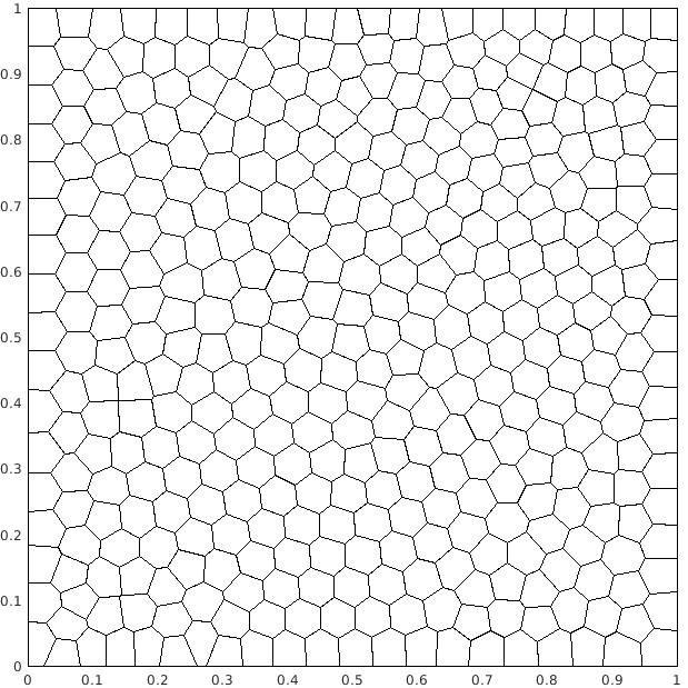
(a) Polymesher

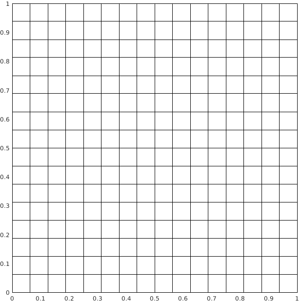
(b) Cartesian

Figure 1: Meshes used in tests.

3.1 Test case 1

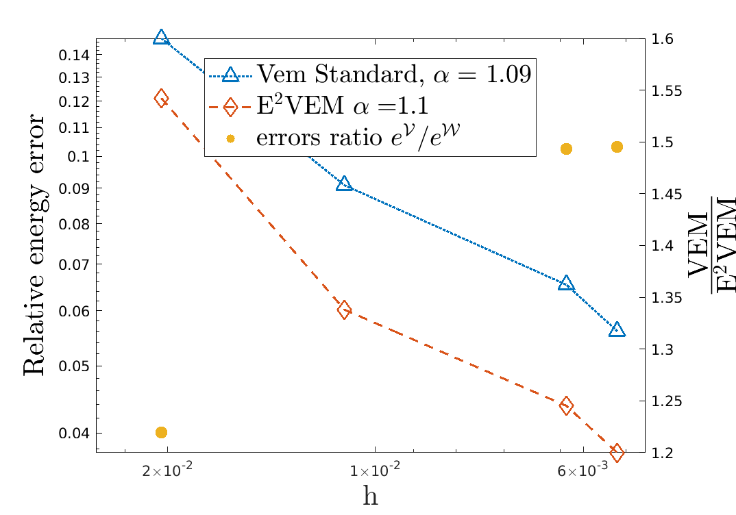
(a) Order 1, Polymesher mesh

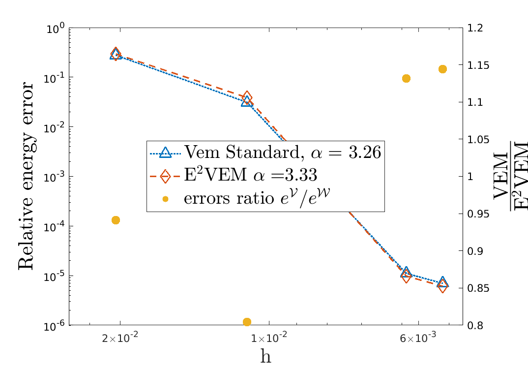
(b) Order 3, Polymesher mesh

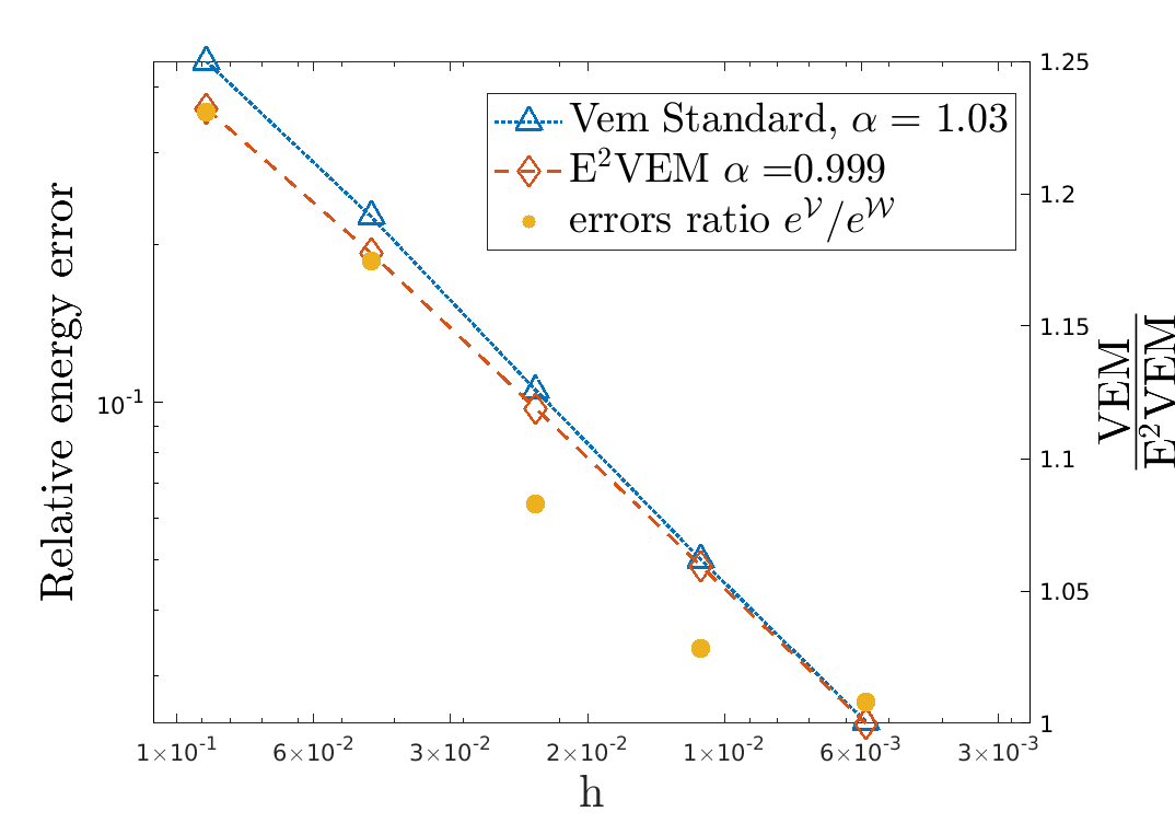
(c) Order 1, Cartesian mesh

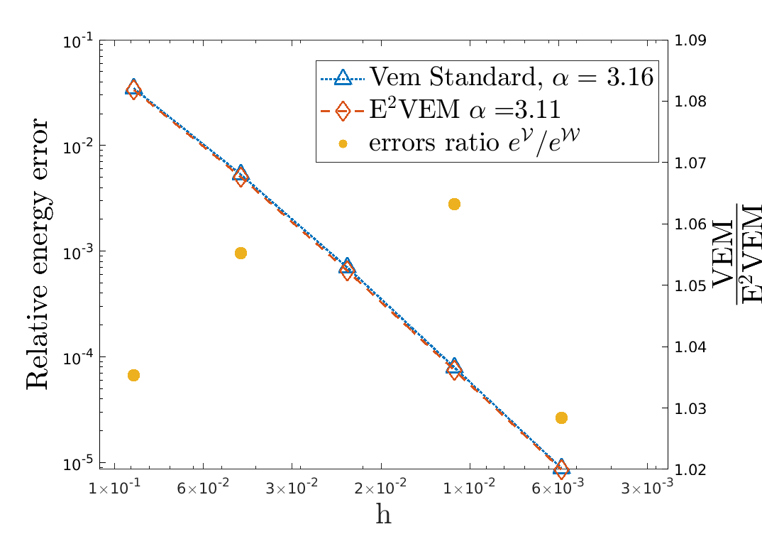
(d) Order 3, Cartesian mesh

Figure 2: Test case 1. Convergence plots.

	Cartesian		Polymesher
	order 1	order 3	order 1	order 3
$\mathrm{avg}\dfrac{\left\lVert{\mathbb{A}^{S}}\right\rVert_{\infty}}{\left\lVert{\mathbb{A}^{\Pi}}\right\rVert_{\infty}}$	1.00	0.23	1.05	0.27

Table 1: Test case 1. Average ratio through refinement between the infinity norms of the polynomial part $\mathbb{A}^{\Pi}$ and the stabilizing part $\mathbb{A}^{S}$ of the stiffness matrix in standard VEM.

In the first test, we define the forcing term $f$ such that the exact solution is $u(x,y)=10^{-2}xy(1-x)(1-y)(\mathrm{e}^{20x}-1)$, whereas $\mathcal{K}=8\cdot 10^{-3}(e_{1}e_{1}^{\intercal})+e_{2}e_{2}^{\intercal}$, where $e_{1}$ and $e_{2}$ are the vectors of the canonical basis of $\mathbb{R}^{2}$. Figure 2 displays the behaviour of the errors obtained with the two methods and the ratio $e^{\mathcal{V}}/e^{\mathcal{W}}$, for orders 1 and 3, with respect to the maximum diameter of the discretization. The results show that the two methods behave equivalently on cartesian meshes, whereas E²VEM performs better on the Polymesher meshes with order $1$, while the two methods tend to have the same behaviour with higher orders. This is due to the strong anisotropy both of the solution (that presents a strong boundary layer in the $x$-direction close to the boundary $x=1$ of the domain) and of the diffusivity tensor $\mathcal{K}$. Indeed, as we can see from Table 1, for $k=1$ the stabilizing part of the VEM bilinear form is of the same order of magnitude as the polynomial part, while for $k=3$ we can see that the polynomial part is predominant. This induces larger errors (see Figure 2(a)) for the standard method on general polygonal meshes, such as the ones in the Polymesher family, since the stabilization is an isotropic operator. This effect is not felt by the E²VEM method since its bilinear form consists only on a polynomial part that correctly takes into account the anisotropy of the tensor $\mathcal{K}$. The difference between the two methods is mitigated on Cartesian meshes since they are by construction aligned with the principal directions of the error (see the error analysis done in [2]).

3.2 Test case 2

(a) Order 1, Polymesher mesh

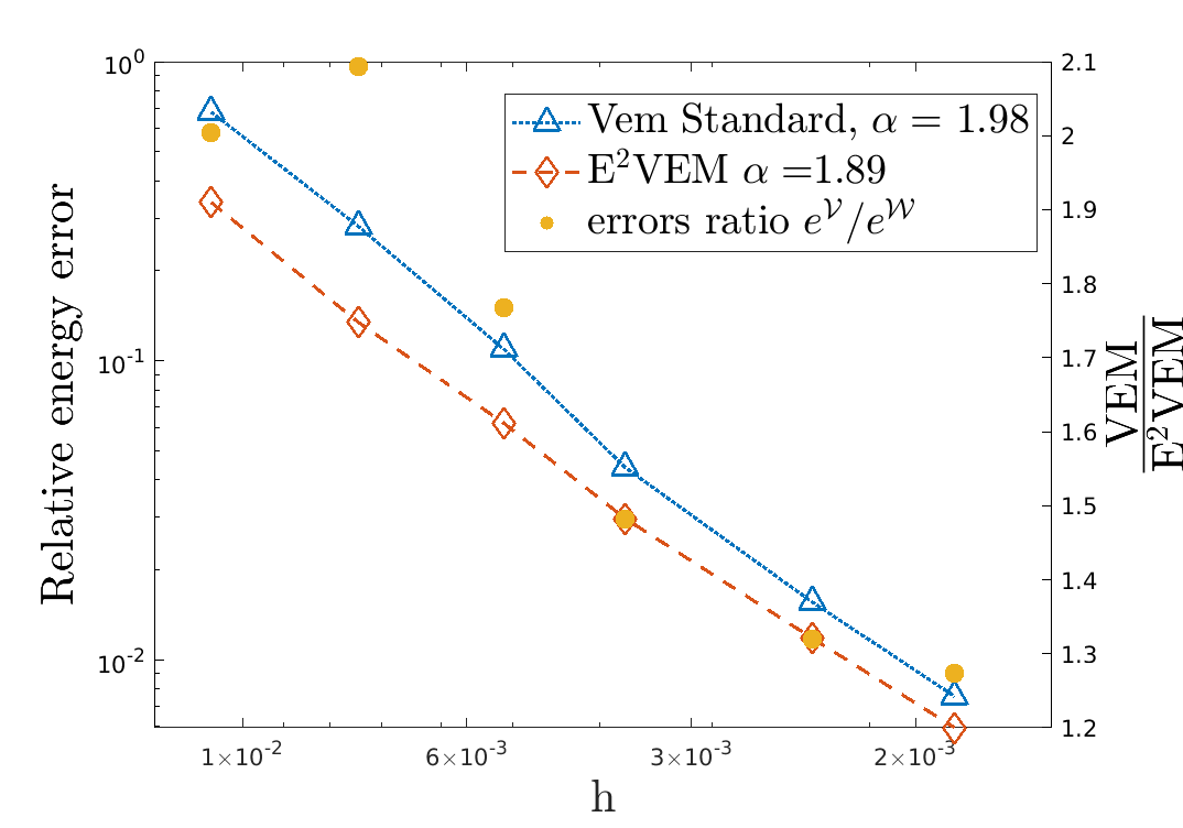
(b) Order 2, Polymesher mesh

Figure 3: Test case 2. Convergence plots.

	Cartesian		Polymesher
	order 1	order 2	order 1	order 2
$\mathrm{avg}\dfrac{\left\lVert{\mathbb{A}^{S}}\right\rVert_{\infty}}{\left\lVert{\mathbb{A}^{\Pi}}\right\rVert_{\infty}}$	1.00	0.56	1.11	0.62

Table 2: Test case 2. Average ratio through refinement between the infinity norms of the polynomial part $\mathbb{A}^{\Pi}$ and the stabilizing part $\mathbb{A}^{S}$ of the stiffness matrix in standard VEM.

In the second test, the exact solution is $u(x,y)=\sin(2\pi x)\sin(80\pi y)$ and $\mathcal{K}=e_{1}e_{1}^{\intercal}+6.25\cdot 10^{-4}(e_{2}e_{2}^{\intercal})$. In Figure 3 we display the error plots for orders 1 and 2 and Table 2 reports again the average ratio between the polynomial and stabilizing parts of the standard VEM bilinear form. The results are mostly consistent with the previous test, hence the convergence plots for Cartesian meshes are not reported for brevity. However, we observe from Figure 3(a) that with Polymesher meshes the E²VEM method reaches the asymptotic rate of convergence before the standard VEM method. This is due to the very strong anisotropy of the solution, due to its highly oscillating behaviour in the $y$-direction.

4 Conclusions

In this letter, we compared the behaviour of standard VEM and E²VEM on some Laplace test problems. Numerical results show that in the presence of strong anisotropies of the solution and diffusivity tensor, when we apply the two methods on general polygonal meshes, E²VEM perform better than VEM in lowest order. In all the other cases, the two methods behave equivalently.

References

• [1] B. Ahmad, A. Alsaedi, F. Brezzi, L. D. Marini, and A. Russo. Equivalent projectors for virtual element methods. Comput. Math. Appl., 66:376–391, September 2013.
• [2] P. F. Antonietti, S. Berrone, A. Borio, A. D’Auria, M. Verani, and S. Weisser. Anisotropic a posteriori error estimate for the virtual element method. IMA J. Numer. Anal., 02 2021.
• [3] L. Beirão da Veiga, F. Brezzi, A. Cangiani, G. Manzini, L. D. Marini, and A. Russo. Basic principles of virtual element methods. Math. Models Methods Appl. Sci., 23(01):199–214, 2013.
• [4] L. Beirão da Veiga, F. Brezzi, L. D. Marini, and A. Russo. Virtual element methods for general second order elliptic problems on polygonal meshes. Math. Models Methods Appl. Sci., 26(04):729–750, 2015.
• [5] Stefano Berrone, Andrea Borio, and Francesca Marcon. Lowest order stabilization free Virtual Element Method for the Poisson equation, 2021.
• [6] C. Talischi, G. H. Paulino, A. Pereira, and I. F. M. Menezes. Polymesher: A general-purpose mesh generator for polygonal elements written in matlab. Struct. Multidiscipl. Optim., 45(3):309–328, 2012.