Chandra follow-up of the Hectospec Cluster Survey: comparison of caustic and hydrostatic masses and constraints on the hydrostatic bias

Abstract

Context. Clusters of galaxies are powerful probes with which to study cosmology and astrophysics. However, for many applications, an accurate measurement of a cluster’s mass is essential. A systematic underestimate of hydrostatic masses from X-ray observations (the so-called hydrostatic bias) may be responsible for tension between the results of different cosmological measurements.

Aims. We compare X-ray hydrostatic masses with masses estimated using the caustic method (based on galaxy velocities) in order to explore the systematic uncertainties of both methods and place new constraints on the level of hydrostatic bias.

Methods. Hydrostatic and caustic mass profiles were determined independently for a sample of 44 clusters based on Chandra observations of clusters from the Hectospec Cluster Survey. This is the largest systematic comparison of its kind. Masses were compared at a standardised radius ($R_{500}$) using a model that includes possible bias and scatter in both mass estimates. The systematics affecting both mass determination methods were explored in detail.

Results. The hydrostatic masses were found to be systematically higher than caustic masses on average, and we found evidence that the caustic method increasingly underestimates the mass when fewer galaxies are used to measure the caustics. We limit our analysis to the 14 clusters with the best-sampled caustics where this bias is minimised ($\geq 210$ galaxies), and find that the average ratio of hydrostatic-to-caustic mass at $R_{500}$ is $M_{500,X}/M_{500,C}=1.12^{+0.11}_{-0.10}$.

Conclusions. We interpret this result as a constraint on the level of hydrostatic bias, favouring small or zero levels of hydrostatic bias (less than $20\%$ at the $3\sigma$ level). However, we find that systematic uncertainties associated with both mass estimation methods remain at the $10-15\%$ level, which would permit significantly larger levels of hydrostatic bias.

1 Introduction

Galaxy clusters are the largest gravitationally bound objects in the Universe, and thus they are used to study the growth of cosmic structures and as cosmological probes. Tight constraints on cosmological parameters can be determined from measurements of the mass function of clusters, or their baryon fraction, as a function of redshift (see e.g. Allen et al., 2011, for a review). However, the accuracy of these constraints crucially depends on the accuracy with which cluster masses can be measured. For example, the exponential drop in the number density of clusters at high masses means that their mass function is a sensitive cosmological probe, but an error of $\sim$ 10% on the cluster mass can lead to a factor of two difference in the expected space density. The measurement of galaxy cluster masses is challenging, as most of the cluster mass is in the form of dark matter. Mass estimation techniques thus probe the masses of clusters indirectly via the effect of the gravitational potential of the cluster on its intracluster medium (ICM), its member galaxies, or images of background galaxies.

Optical data were used to give the first mass estimates of galaxy clusters. Zwicky (1933) measured the line-of-sight velocities of a number of cluster galaxies in the nearby Coma cluster, and, by computing the velocity dispersion, used the virial theorem to estimate a mass for the cluster. In the late 1960s and 1970s, the first X-ray satellites were launched, and it was in the 1990s that the first X-ray samples of hundreds of clusters were produced (Ebeling et al., 1998, 2001; Böhringer et al., 2000, 2001) from which X-ray hydrostatic masses could be calculated (e.g. Reiprich & Böhringer, 2002). The launch of XMM-Newton and Chandra in 1999 has led to even more precise X-ray masses being measured for large samples of clusters (e.g. Martino et al., 2014). The first work using weak gravitational lensing (WL) to map the dark matter distribution, undertaken by Tyson et al. (1990), was followed by a number of other papers (e.g. Blandford et al., 1991; Miralda-Escude, 1991; Kaiser, 1992), and in the last 3 decades it has become increasingly common to use WL as a mass estimation technique (see Umetsu, 2020 for a review).

For cosmological studies, the calibration of masses is critical to understand the biases that may be inherent to different mass estimation techniques. Cosmology requires large samples of clusters with masses which in general must be estimated from simple mass proxies that must be calibrated with more direct, higher fidelity mass measurements. Thus, the accuracy of the mass scale from those measurements is crucial, and biases in the mass scale can manifest as biases in the derived cosmological parameters. For example, there is currently tension between the cosmological constraints ($\Omega_{m}$ and $\sigma_{8}$) from the Planck cluster number counts (Planck Collaboration et al., 2016a) and the Planck cosmic microwave background (CMB) results (Planck Collaboration et al., 2016b). The Planck cluster masses were calibrated using hydrostatic masses, and the tension in the results could be due to a negative bias (i.e. the true mass is underestimated) in the hydrostatic masses, often referred to as the hydrostatic bias.

More recent analyses have found lower tension between the values of $\sigma_{8}$ obtained from the Planck CMB and from cluster number counts measured with SZE or X-ray cluster surveys (e.g. Douspis et al., 2019; Bocquet et al., 2019; Planck Collaboration et al., 2020; Garrel et al., 2022; Salvati et al., 2021). The improved agreement comes from updates to the CMB analysis and the mass calibration of the clusters, with all analyses favouring a non-negligible hydrostatic bias. However the magnitude of the hydrostatic bias is not agreed upon, and remains a critical point for cluster studies.

Some level of hydrostatic bias is expected a-priori, due to the assumption that the only pressure support in the ICM is the thermal pressure measured in X-rays. If any other sources of pressure (e.g. from turbulence, bulk motions or clumping of the ICM, or from cosmic rays) are also present, this leads to the X-ray hydrostatic mass method underestimating the true cluster mass (Nagai et al., 2007; Lau et al., 2009; Nelson et al., 2014).

The level of hydrostatic bias is expected to be higher in unrelaxed clusters compared with relaxed clusters, as unrelaxed systems are expected to have more non-thermal pressure support from bulk motions and turbulence of the cluster gas. However, all clusters, regardless of dynamical state, will experience some amount of non-thermal pressure support, as gas and substructures are always infalling onto the cluster as they undergo constant growth, leading to non-thermal pressure due to the residual motion of the ICM and the turbulence created. Constraining turbulence in the ICM requires high resolution X-ray spectrometry, and the only mission thus far capable of this has been Hitomi. Before the mission failed, Hitomi observed the Perseus cluster, finding that in the core of the Perseus cluster the pressure support from turbulence was 4% of the thermodynamic pressure (Hitomi Collaboration et al., 2016), which on its own would not lead to a large value of hydrostatic bias (though we note that the Perseus cluster is a dynamically relaxed cluster and, of course, not representative of the cluster population as a whole).

The hydrostatic bias may also be a function of radius, as the infalling gas may lead to stronger gas motions and therefore significant non-thermal pressure support at the outskirts of clusters. Bonamente et al. (2013) and Fusco-Femiano & Lapi (2018) both find evidence for significant non-thermal pressure at the cluster outskirts (for A1835 and A2142 respectively), and work using hydrodynamical simulations suggests that the non-thermal pressure due to the bulk gas motion increases with radius (Nagai et al., 2007; Lau et al., 2009; Vazza et al., 2009, 2018; Battaglia et al., 2012; Rasia et al., 2012). Specifically, Nagai et al. (2007) and Rasia et al. (2012) both find that at low ($<$ 0.2 $R_{500}$) and high radius ($>$ $R_{500}$) the bias increases. Nagai et al. (2007) find the bias to increase from $<$10% at $R_{500}$ to $\sim$ 30% at twice this radius. Studies that have used observational data agree with this general trend (Siegel et al., 2018; Eckert et al., 2019).

To get a grasp on the biases of the cluster mass estimation methods, comparisons between methods themselves are undertaken, and simulated data are also used to compare the known mass from the simulation to the mass that is recovered if observational methods are applied to synthetic observations of the simulated cluster. Comparisons of X-ray hydrostatic masses with WL masses can yield insights into the magnitude of the hydrostatic bias, as WL masses are not sensitive to the state of the ICM (in contrast to X-ray hydrostatic masses). However, WL masses are sensitive to mass along the line of sight to the observed cluster, which can lead to scatter of $\sim$ 20 - 30% and positive bias of up to $\sim$ 20% (Hoekstra, 2001, 2003; Hoekstra et al., 2011; Becker & Kravtsov, 2011; Hwang et al., 2014), which needs to be understood and taken into account in these comparisons. A further complication is that the uncertainty on WL masses increases with decreasing cluster mass and decreasing cluster redshift (Hoekstra, 2003), and even for a cluster with mass 5$\times$10¹⁴ $\text{M}_{\odot}$ at a redshift of 0.3, the one sigma uncertainty can be as large as 40%. Some comparisons between WL masses and X-ray hydrostatic masses suggest that X-ray hydrostatic masses underestimate the true mass by $\sim$ 20 - 30% (von der Linden et al., 2014; Donahue et al., 2014; Sereno et al., 2015; Hoekstra et al., 2015). Work using hydrodynamical simulations also suggest a significant hydrostatic bias of $\sim$10 - 30% (Rasia et al., 2006, 2012; Nagai et al., 2007; Lau et al., 2009; Nelson et al., 2014). However Gruen et al. (2014), Israel et al. (2014), Applegate et al. (2016) and Smith et al. (2016) find no significant evidence for hydrostatic bias when comparing X-ray hydrostatic masses to WL masses.

Comparisons between X-ray and WL masses from observations also support the idea that disturbed clusters will have a larger hydrostatic bias than relaxed clusters (Zhang et al., 2010; Mahdavi et al., 2013). Biffi et al. (2016) also find a difference in hydrostatic bias between relaxed and disturbed clusters using simulations (though find no difference between cool core and non cool core systems).

Comparisons between X-ray and caustic masses are much rarer. Caustic masses (Diaferio & Geller, 1997; Diaferio, 1999) are a useful alternative to WL masses for testing the accuracy of hydrostatic masses. Like WL masses they are not sensitive to the state of the ICM, and biases in the caustic method are, in principle, well understood from simulations (Serra et al., 2011). One drawback of using caustic masses for comparison is that they have a large scatter of $\sim$ 30% (Serra et al., 2011), which comes predominantly from the assumption of spherical symmetry (and thus the viewing angle of the cluster). Thus, for a meaningful comparison, a large cluster sample is needed (several tens of clusters). Another drawback of the comparison is that the caustic mass method was conceived to measure the mass in the outer region of clusters, from 1 - 3 $R_{200}$, where the X-ray hydrostatic mass method cannot be applied because the X-ray surface brightness is too low to return a reliable signal at these radii. However, Serra et al. (2011) use simulations to estimate the bias in the caustic method at lower radii, such that a meaningful comparison between the two cluster mass estimators can still be made.

Diaferio et al. (2005) was the first work to compare X-ray and caustic masses, for a sample of three clusters, finding that for two clusters the mass profiles agreed well, and for the other cluster they did not, as the cluster was clearly out of equilibrium. Much larger cluster samples (from observational data) were used by Maughan et al. (2016), Andreon et al. (2017a) and Foëx et al. (2017) to infer caustic masses to be $\sim$20% lower (at $R_{500}$), $\sim$15% larger (at $R_{500}$) and $\sim$30% larger (at $R_{200}$) than the hydrostatic masses respectively. Armitage et al. (2019) use simulation data to compare caustic and X-ray hydrostatic masses (at $R_{200}$) and find a similar mass ratio to Foëx et al. (2017). Ettori et al. (2019), however, find their caustic masses to be underestimated by $\sim$ 40% (at $R_{200}$) compared to their hydrostatic masses (both computed using observational data). These contradictory results clearly show that the situation is complex and unsettled.

There have also been comparisons of caustic masses with weak lensing - Diaferio et al. (2005) do so for a sample of three clusters, and Geller et al. (2013) do so for a sample of 19 clusters. Both works find the mass methods to agree (independent of the dynamical state of the cluster) at around the virial radius to within $\sim$ 30%, consistent within the errors associated with each mass method.

In this paper, we aim to compare hydrostatic and caustic masses for the largest sample so far used for these purposes, in order to investigate the accuracy of the methods and provide new constraints on the hydrostatic bias that are independent of those based on WL masses. We improve on our earlier work (Maughan et al., 2016) by expanding the sample from 16 to 44 clusters. We also include a more comprehensive analysis of the systematics, and our main conclusions are based on a subset of 14 clusters for which the systematics are minimised.

In this paper we use the following notation to represent the masses of the clusters. $M_{X}$ and $M_{C}$ denote the masses measured with the hydrostatic and caustic methods, respectively. When these masses are specifically measured within $R_{\text{500}}$, we denote them as $M_{500,X}$ and $M_{500,C}$. Unless otherwise stated, these are always measured within the $R_{\text{500}}$ determined from the hydrostatic analysis.

The structure of the paper is as follows. In §2 we discuss the sample selection and data preparation. §3 details the data analysis and modelling. In §4 we present initial results for the full sample, and then our main results from the subset found to have the most reliable mass estimates. We discuss our results in §5, including a review of the systematics affecting the mass estimates, and the implications for the hydrostatic bias, and summarise our findings in §6. Throughout this paper we assume a WMAP9 cosmology of $H_{0}=69.7$ km s^-1Mpc^-1, $\Omega_{\Lambda}=0.718$, and $\Omega_{m}=0.282$ (Hinshaw et al., 2013). All measurement uncertainties correspond to 68% confidence level, unless explicitly stated otherwise. When referring to base 10 logarithm we use ‘$\log$’ or ‘$\log_{10}$’, and use ‘$\ln$’ if referring to the natural logarithm.

2 Cluster sample

For our analysis, we used the X-ray flux-limited subset of the Hectospec Cluster Survey (HeCS; Rines et al., 2013), a spectroscopic survey of X-ray selected clusters. The HeCS sample was constructed by matching clusters selected using the ROSAT All-Sky Survey (RASS; Voges et al., 1999) with the imaging footprint of the SDSS Data Release 6 (Adelman-McCarthy et al., 2008). The SDSS data were used to select candidate cluster member galaxies for spectroscopic follow-up, which was performed with MMT/Hectospec (Fabricant et al., 2005).

The X-ray flux limit applied to the HeCS sample in order to create the flux-limited HeCS sub-sample was $5\times 10^{-12}\mbox{$\text{\leavevmode\nobreak\ erg}$}\mbox{$\text{\leavevmode\nobreak\ s}$}^{-1}\mbox{$\text{\leavevmode\nobreak\ cm}$}^{-2}$ (in the $0.1-2.4\mbox{$\text{\leavevmode\nobreak\ keV}$}$ band), which excluded A750, A2187, A2396, A2631, and A2645 from the full HeCS sample. We then excluded three clusters from the flux-limited sample that were found to be clearly dominated by AGN upon inspection of available X-ray observations (these were A689 and A1366 based on Chandra data, and A2055 based on XMM-Newton data). More specifically, A1366 and A2055 have BLLacs in the brightest cluster galaxy (BCG), and A689 has a BLLac very close to the BCG (Giles et al., 2012). This resulted in a flux-limited sample of 50 clusters. We then obtained Chandra follow-up observations of those clusters lacking Chandra data.

To construct the final sample, we then excluded four clusters due to flaring in the available Chandra observations (A267, A667, A1361, and A1902), one cluster as it was part of a double cluster (A1758), and one cluster as it was off-chip in the Chandra observation available (A646 - the observation was of a radio galaxy in the cluster, but around 7^′ from the cluster core). The final sample then consists of 44 clusters, which are summarised in Table 1. All clusters are in the redshift range $0.1<$ z $<0.3$. We call our sample the CHeCS (Chandra observations of Hectospec Cluster Survey clusters) sample. We note that the masses from Rines et al. (2013) were converted to be consistent with the value of $H_{0}$ we use in this paper.

Cluster	Short name	RA	DEC	z	ObsID	clean time	Ngal
		deg	deg			(ks)
ZwCl 0755.8+5408	Zw1478	119.9190	53.9990	0.1027	18248	20	82
Abell 0655	A655	126.3610	47.1320	0.1271	15159	8	315
Abell 0697	A697	130.7362	36.3625	0.2812	4217	20	185
MS 0906.5+1110	MS0906	137.2832	10.9925	0.1767	924	30	101
Abell 0773	A773	139.4624	51.7248	0.2173	5006,533,3588	15,10,9	173
Abell 0795	A795	141.0240	14.1680	0.1374	11734⋆	29	179
ZwCl 0949.6+5207	Zw2701	148.1980	51.8910	0.2160	12903⋆,3195⋆	93,22	93
Abell 0963	A963	154.2600	39.0484	0.2041	903⋆	34	211
Abell 0980	A980	155.6275	50.1017	0.1555	15105	14	222
ZwCl 1021.0+0426	Zw3146	155.9117	04.1865	0.2894	909,9371	43,33	106
Abell 0990	A990	155.9120	49.1450	0.1416	15114	10	91
ZwCl 1023.3+1257	Zw3179	156.4840	12.6910	0.1422	13375	9	69
Abell 1033	A1033	157.9320	35.0580	0.1220	15614,15084	33,29	191
Abell 1068	A1068	160.1870	39.9510	0.1386	1652⋆	26	129
Abell 1132	A1132	164.6160	56.7820	0.1351	19770,13376	20,9	160
Abell 1201	A1201	168.2287	13.4448	0.1671	9616	47	165
Abell 1204	A1204	168.3324	17.5937	0.1706	2205	24	92
Abell 1235	A1235	170.8040	19.6160	0.1030	18247	18	131
Abell 1246	A1246	170.9912	21.4903	0.1921	11770	5	226
Abell 1302	A1302	173.3070	66.3990	0.1152	18245	19	162
Abell 1413	A1413	178.8260	23.4080	0.1412	5003	75	116
Abell 1423	A1423	179.3420	33.6320	0.2142	11724,538	26,10	230
Abell 1437	A1437	180.1040	03.3490	0.1333	15306,15188	10,9	194
Abell 1553	A1553	187.6959	10.5606	0.1668	12254	9	171
Abell 1682	A1682	196.7278	46.5560	0.2272	11725	20	151
Abell 1689	A1689	197.8750	- 1.3353	0.1842	6930,7289,5004	76,75,20	210
Abell 1763	A1763	203.8257	40.9970	0.2312	3591	20	237
Abell 1835	A1835	210.2595	02.8801	0.2506	6880,6881,7370	118,36,40	219
Abell 1918	A1918	216.3420	63.1830	0.1388	18249	21	80
Abell 1914	A1914	216.5068	37.8271	0.1660	20026,18252,20023,20025,20024	29,27,25,22,17	255
Abell 1930	A1930	218.1200	31.6330	0.1308	11733⋆	35	76
Abell 1978	A1978	222.7750	14.6110	0.1459	18250	20	63
Abell 2009	A2009	225.0850	21.3620	0.1522	10438	20	195
RXCJ 1504.1-0248	RXJ1504	226.0321	- 2.8050	0.2168	17670,17197,17669,4935	51,30,29,12	120
Abell 2034	A2034	227.5450	33.5060	0.1132	12886,12885	91,81	182
Abell 2050	A2050	229.0680	00.0890	0.1191	18251	15	106
Abell 2069	A2069	231.0410	29.9210	0.1139	4965	39	441
Abell 2111	A2111	234.9337	34.4156	0.2291	11726, 544	21,10	208
Abell 2219	A2219	250.0892	46.7058	0.2257	14356,14431,14355,14451	49,39,30,20	461
ZwCl 1717.9+5636	Zw8197	259.5480	56.6710	0.1132	18246	19	76
Abell 2259	A2259	260.0370	27.6702	0.1605	3245	10	165
RXCJ 1720+2638	RXJ1720	260.0370	26.6350	0.1604	4361,1453	14,8	376
Abell 2261	A2261	260.6129	32.1338	0.2242	5007	24	209
RXCJ 2129+0005	RXJ2129	322.4186	00.0973	0.2339	9370,552	30,10	325

Table 1: Summary of sample. Column 1 gives the cluster name with a shorter alternative name given in column 2, columns 3 and 4 give the RA and DEC of the cluster respectively, column 5 gives the spectroscopic redshift of the cluster, column 6 gives the Chandra ObsID(s), column 7 gives the length of the observation after lightcurve cleaning, column 8 gives the number of galaxies classed as member galaxies of each cluster in the caustic method (Serra & Diaferio, 2013), as defined in Rines et al. (2013) (equivalent to the number of galaxies within the caustics). Starred ObsIDs are ACIS-S otherwise all are ACIS-I

3 Analysis

3.1 X-ray data

The Chandra data analysis follows closely that presented in Giles et al. (2015), which in turn is based on the analysis presented in Maughan et al. (2008) and Maughan et al. (2012). We summarise the main steps here, and highlight any differences in the updated analysis used in this paper. Any peculiarities of the analysis of individual clusters are noted in Appendix A.

All of the clusters in our sample were analysed with the ciao 4.10 software package and caldb version 4.8.1 (Fruscione et al., 2006). Projected emissivity profiles of the ICM were obtained from the surface brightness profile, measured in circular annuli centred on the centroid of the X-ray emission. The centroid location was measured in an X-ray image produced in the $0.7-2\mbox{$\text{\leavevmode\nobreak\ keV}$}$ band, and was determined by iteration using a circular region of $150\mathrm{{}^{\prime}}\hskip-1.00006pt\mathrm{{}^{\prime}}$ and then $50\mathrm{{}^{\prime}}\hskip-1.00006pt\mathrm{{}^{\prime}}$ initially centred on the X-ray peak (Maughan et al., 2008). Projected temperatures profiles were obtained by extracting spectra in circular annuli also centred on the X-ray centroid. The spectra were fit with an absorbed APEC plasma model (Smith et al., 2001) in XSPEC (Arnaud, 1996). For the spectral analysis, instead of using the $\chi^{2}$ statistic as in Maughan et al. (2016), we used the C-statistic, which assumes Poissonian statistics, and the spectra were grouped to contain at least five counts per energy bin. This minimal binning is required to avoid a bias in the XSPEC implementation of the C-statistic when there are bins in the spectrum with zero or very few counts (see Willis et al., 2005, and the discussion in Appendix B in the XSPEC manual). We exclude the outermost temperature measurement in the profile if the measured temperature in the final bin is greater than 15 keV, has errors $>$50%, or including it leads to an unphysical increase in the best fit temperature profile.

A further minor difference from our previous analysis is that the absorbing column used in the spectral fits are fixed at the nhtot value from Willingale et al. (2013), instead of the absorbing column from Dickey & Lockman (1990). The updated nhtot value now contains absorption contributions from molecular hydrogen, not previously accounted for. We note this update does not significantly affect our results.

In order to calculate hydrostatic mass profiles, we use the models for the 3D temperature and gas density profiles as presented in Vikhlinin et al. (2006) and fit them to the observed projected temperature profile and surface brightness profile respectively (this mass fitting method is sometimes referred to as the forward-fitting mass method e.g. Ettori et al., 2013 and more details of our implementation are given in Appendix B). In this work we fit the 3D temperature and gas density models simultaneously, in contrast to the X-ray mass method used in Maughan et al. (2016). This fitting is done using a Markov Chain Monte Carlo (MCMC) method using emcee (Foreman-Mackey et al., 2013), and the priors used on the 3D gas density and temperature models are presented in Table 2. Uncertainties on the mass profile are obtained straightforwardly from the MCMC chains. We also compute the mean $R_{500}$, and mean hydrostatic mass at $R_{500}$ from these chains (presented in Table 3). Gas mass profiles can also be obtained from the 3D gas density fit, with uncertainties obtained from the MCMC chains in the same way. This means that the uncertainties derived on the gas mass within $R_{\text{500}}$ self-consistently include the uncertainties on $R_{\text{500}}$.

Density profile
$n_{0}$	$r_{\text{c}}$	$r_{\text{s}}$	$\alpha$	$\beta$	$\epsilon$	$n_{02}$	$r_{\text{c2}}$	$\beta_{2}$
cm-3	kpc	kpc				cm-3	kpc
($10^{-4}$, $10^{-1}$)	(5, 800)	(100, 4000)	(0, 3)	(0.3, 1.5)	(0, 5)	(0, $10^{-1}$)	(1, 70)	(0.1, 5)
Temperature profile
$T_{\text{0}}$	$r_{\text{cool}}$	$a_{\text{cool}}$	$T_{\text{min}}$	$r_{\text{t}}$	a	b	c
keV	kpc		keV	kpc
(0.5, 18)	(10, 500)	(0, 3)	(0.1, 6 or $T_{\text{0}}$)	(100, 500)	(-0.5, 0.5)	(0, 5)	(0, 1)

Table 2: Summary of priors for the 3D gas density and 3D temperature models (see §B for equations) used in the X-ray hydrostatic mass method described in §3.1. All are flat uniform priors (in linear space) with lower and upper bounds in parentheses.

To investigate the influence of the clusters’ dynamical states on our results, we split our sample into relaxed cool core (RCC) and non-relaxed cool core (NRCC) clusters, using the same three diagnostics as in Maughan et al. (2016). To be classed as RCC, a cluster has to have a low central cooling time ($<$ 7.7 Gyr), a highly peaked central density profile (logarithmic slope $>$ 0.7 within 0.048 $R_{500}$), and a low centroid shift ($<$ 0.009). This definition of what constitutes a RCC cluster is a conservative one: for our sample of 44 clusters, 10 are classified as RCC (see Table 3).

This work is an extension of Maughan et al. (2016) from 16 to 44 clusters. As noted §2, we have dropped A267 and A2631 from the present analysis, leaving 14 clusters in common. For these clusters, we compared the hydrostatic masses at $R_{500}$ between the two analyses, finding a weighted average ratio of the new masses to those from Maughan et al. (2016) of 0.96$\pm$0.05. This demonstrates that the improvements in our analysis, and changes to the Chandra calibration have not significantly affected our hydrostatic mass estimates.

3.2 Caustic masses

In this work, we use the caustic masses from HeCS, as presented in Rines et al., 2013. We summarise the key aspects of the analysis in the following. The caustic mass method uses spectroscopic redshifts for a number of member galaxies in a cluster (on average $\sim$180 for our sample, see column 7 Table 1), to determine their line-of-sight velocity (relative to the median of the distribution of the line-of-sight velocities of the galaxies of the main group on the binary tree Diaferio, 1999), which when combined with their projected distances from the cluster centre, can be used to estimate a mass profile of a cluster.

By plotting the line-of-sight velocity versus the projected distance from the cluster centre for each of the member galaxies (referred to as a redshift diagram), an overpopulated region of this parameter space is clearly seen (see e.g. Rines et al., 2013), and is bounded by a ‘trumpet shape’. The boundaries between galaxies within this trumpet shape and outside it are known as caustics. The galaxies within this overpopulated parameter space are assumed to be bound by the cluster’s gravitational potential, and their velocities are assumed to be less than the escape velocity of the cluster. The amplitude, ${\cal A}(r)$, of this trumpet shape is related to the cluster’s escape velocity and the velocity anisotropy parameter $\beta(r)$, and decreases as a function of projected distance from the cluster centre. Diaferio & Geller (1997) show that this caustic amplitude, ${\cal A}(r)$, can be related to the cluster mass within a radius, $r$:

$$GM(<r)=\mathcal{F}_{\beta}\int_{0}^{r}{\cal A}^{2}(r)\,dr\,.$$ (1)

Equation (1) simplifies the correct equation $GM(<r)=\int_{0}^{r}{\cal F}_{\beta}(r){\cal A}^{2}(r){\mathrm{d}}r$ by replacing the function ${\cal F}_{\beta}(r)$ with the constant filling factor ${\cal F}_{\beta}$. The function ${\cal F}_{\beta}(r)$ combines the cluster density profile and the anisotropy of the velocity field, both of which vary as a function of $r$. Beyond $\sim 0.5R_{200}$, ${\cal F}_{\beta}(r)$ is roughly constant with radius, so assuming a constant filling factor ${\cal F}_{\beta}$ should not lead to significant overestimation or underestimation of mass at larger radii (Diaferio, 1999). However, within $\sim 0.5R_{200}$, approximating ${\cal F}_{\beta}(r)$ to a constant might lead to an overestimate of the cluster mass by $\sim 15\%$ (Serra et al., 2011).

We note that we use $\mathcal{F}_{\beta}=0.5$ for the filling factor, which is appropriate for the algorithm of Diaferio (1999) used to calculate the caustic masses presented in Rines et al. (2013).

The uncertainties on the caustic masses represent the statistic precision of the caustic mass estimate due to the uncertainties in the location of the caustics. They do not represent the accuracy with which the caustic mass measures the true mass, which is $\approx 30\%$ (Serra et al., 2011), driven largely by the effects of projection and the viewing angle of the cluster (this is accounted for in our model below by an intrinsic scatter between caustic and true masses).

The uncertainty on the caustic location increases with decreasing ratio $\rho$ between the number of galaxies within the caustics and the number of galaxies in the redshift diagram. On average, this recipe is a robust estimate of the statistical uncertainty (Serra et al., 2011). However, in sparsely-sampled redshift diagrams, the caustic technique might underestimate the statistical uncertainty, because the ratio $\rho$ might remain relatively large, despite the low number of galaxies in the diagram. We verified that these cases have a negligible effect on our results by repeating our analysis with a uniform $50\%$ error on all caustic masses. In this test, the intrinsic scatter term in our model is effectively removed and we prevent any points with underestimated errors from driving the results.

The number of galaxies within the caustics, Ngal, can also have a systematic effect on the mass derived using the caustic method. The simulations of Serra et al. (2011) suggest an underestimate of the mass of $\sim 10\%$ at $R_{500}$ for $\text{Ngal}\sim 100$, with the masses being unbiased for $200\,\hbox to0.0pt{\raise 1.72218pt\hbox{$<$}\hss}{\lower 2.58334pt\hbox{$\sim$}}\,\text{Ngal}\,\hbox to0.0pt{\raise 1.72218pt\hbox{$<$}\hss}{\lower 2.58334pt\hbox{$\sim$}}\,1000$. Any underestimate of mass due to low values of Ngal is expected to approximately cancel with the overestimate of mass at $R_{500}$ due to the assumption of constant filling factor. However, as discussed below (§4.2), our results suggest that the magnitude of the mass underestimate for low values of Ngal may be larger than predicted, and our main conclusions are thus based on the clusters with the largest values of Ngal.

3.3 Modelling the mass biases

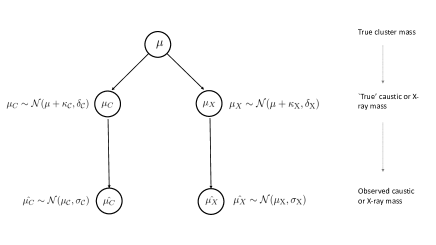
Figure 1: Graphical model summarising the mass modelling framework that we present in §3.3. The symbols are also described in that section; in summary, the symbol $\mu$ represents mass, $\kappa$ is the bias term, $\delta$ is the scatter term and $\sigma$ is the measurement error term (all in log space), and the $C$ and $X$ subscripts denote whether the quantity refers to that from the hydrostatic or caustic method. The $\hat{}$ refers to an observed quantity. $\cal{N}$ refers to a normal distribution, and ‘$\sim$’ denotes ‘is distributed as’.

In order to constrain the bias and scatter between the hydrostatic and caustic mass measurement techniques, we use a Bayesian framework (of which a graphical representation is shown in Figure 1). The modelling framework is the same as in Maughan et al. (2016), but we summarise the key points here. In the following, we use $\mu$ to denote the base 10 logarithm of mass.

A given cluster with a ‘true’ mass, $\mu$ also has a ‘true’ caustic mass, $\mu_{C}$, and ‘true’ hydrostatic mass, $\mu_{X}$, which are related to the true mass, $\mu$, as follows:

$$\mu_{X}\sim\cal{N}(\mu+\rm\kappa_{X},\rm\delta_{X})$$ (2)

$$\mu_{C}\sim\cal{N}(\mu+\rm\kappa_{C},\rm\delta_{C})$$ (3)

where $\kappa_{X}$ and $\kappa_{C}$ parametrise the bias between the true mass and the ‘true’ hydrostatic and caustic mass, respectively, and $\delta_{X}$ and $\delta_{C}$ parametrise the intrinsic scatter between the true mass and the ‘true’ hydrostatic and caustic mass, respectively. $\cal{N}$ refers to a normal distribution, and “$\sim$” is equivalent to “is distributed as”.

These ‘true’ hydrostatic and caustic masses are related to the observed hydrostatic and caustic masses ($\hat{\mu_{X}}$ and $\hat{\mu_{C}}$, respectively), as follows:

$$\hat{\mu_{X}}\sim\cal{N}(\rm\mu_{X},\rm\sigma_{X})$$ (4)

$$\hat{\mu_{C}}\sim\cal{N}(\rm\mu_{C},\rm\sigma_{C})$$ (5)

where $\sigma_{X}$ and $\sigma_{C}$ represent the standard deviation of the lognormal error for the observed hydrostatic and caustic masses, respectively. Note that our model does not take into account selection effects that could arise due to the X-ray flux limit. However, we show in §5.3 that this has a negligible impact on our results.

We used the same (loose) priors as in Maughan et al. (2016) on the cluster masses, bias and scatter terms. Specifically, for the cluster masses in log space, $\mu$, we applied a uniform prior from 12 to 17. For the bias terms in log space, $\kappa_{X}$ and $\kappa_{C}$, we applied normal priors with mean 0 and a standard deviation of 1. For the intrinsic scatter terms in log space, $\delta_{X}$ and $\delta_{C}$, we applied normal priors (truncated at zero) with mean 0.09 and a standard deviation of 2.2, corresponding to a weak prior with a mean of $\sim$20% in normal space.

Using the model described above, we used the observational data that we have for each cluster ($\hat{\mu_{X}}$, $\sigma_{X}$, $\hat{\mu_{C}}$, $\sigma_{C}$) to constrain the ’true’ hydrostatic and caustic mass terms ($\mu_{X}$, $\mu_{C}$), the scatter terms ($\delta_{X}$ and $\delta_{C}$) and bias terms ($\kappa_{X}$ and $\kappa_{C}$) for all of the clusters in our sample. Both the scatter terms and the bias terms are degenerate, however, the intrinsic scatter between the hydrostatic and caustic mass measurements

$$\delta=\sqrt{\delta_{X}^{2}+\delta_{C}^{2}}$$ (6)

and the mean bias between the hydrostatic and caustic mass measurements

$$\kappa=\kappa_{X}-\kappa_{C}=\mu_{X}-\mu_{C}=\log_{10}\left(\frac{M_{X}}{M_{C}}\right)$$ (7)

can be constrained by the data.

When reporting the values of $\kappa$ and $\delta$ in Tables 4 and 5, we report the median value of $\delta$, with errors given as the difference between the median and the 16th and 84th percentiles. For $\kappa$, we report the mean value. As $\kappa=\log_{10}(M_{X}/M_{C})$, and $\kappa$ (a quantity in log space) is normally distributed, the posterior of $M_{X}/M_{C}$ (a quantity in linear space) is lognormally distributed. Therefore, in Tables 4 and 5 we summarise the posterior of $M_{X}/M_{C}$ by reporting its median and errors in the same way that we did for $\delta$. In these tables, the $\kappa$ values are given in base 10 log space, and the $\delta$ values have been converted to percentage scatters.

We also note that in Table 3 and in all figures showing mass errors, we report the mean and standard deviation of the hydrostatic and caustic mass measurements in linear space, which is the form in which masses are often reported in other work. However, we find that the uncertainties on the mass measurements are in fact better described using lognormal errors, and so choose to model the biases associated with the caustic and X-ray hydrostatic mass measurement methods in log space.

We use the probabilistic programming language stan to implement the model described above, specifically using the No-U-Turn Sampler (Hoffman & Gelman, 2011). We sampled the parameters in our model with four chains of 5,000 steps each. The analysis can be done at any radius, and so by repeating the analysis at increasing radii, we produced a profile of the mean bias between the two mass measurement methods.

In our analysis, the mass determination methods are independent and use different definitions of the cluster centre (the x-ray centroid for the hydrostatic mass, and the peak of the galaxy distribution on the sky and the median of the line-of-sight velocity distribution of the cluster members with the caustic method). This means that the radial coordinates are not identical and a given radius does not correspond to an identical aperture for both methods. For our main analysis, we scale radial coordinates to the $R_{\text{500}}$ estimated from the hydrostatic method. This is motivated by the expectation that the hydrostatic mass should have lower intrinsic scatter with the true mass. We show in §5.2 that using $R_{\text{500}}$ computed independently for each method does not alter our conclusions.

4 Results

In the following, we first present the comparisons between hydrostatic and caustic masses for the full CHeCS sample. We then demonstrate that the caustic masses for clusters with lower values of Ngal are likely to be underestimated. Finally we present our main results, based on the subset of clusters with higher values of Ngal.

4.1 Initial results for the full sample

Cluster	z	Status	$R_{500}$	$M_{500,X}$	$M_{500,C}$	Ngal	Ngal	nhtot
			Mpc	$10^{14}\text{M}_{\odot}$	$10^{14}\text{M}_{\odot}$	sub-sample		cm-2
ZW1478	0.103	NRCC	0.80 $\pm$ 0.03	1.57 $\pm$ 0.27	0.81 $\pm$ 0.04	low	82	3.86
A0655	0.127	NRCC	1.08 $\pm$ 0.04	4.05 $\pm$ 0.83	3.87 $\pm$ 0.20	high	315	4.39
A0697	0.281	NRCC	1.47 $\pm$ 0.05	11.88 $\pm$ 1.81	5.90 $\pm$ 2.80	mid	185	3.28
MS0906	0.177	NRCC	1.04 $\pm$ 0.02	3.74 $\pm$ 0.33	1.78 $\pm$ 0.24	low	101	3.61
A0773	0.217	NRCC	1.32 $\pm$ 0.03	7.97 $\pm$ 0.88	9.78 $\pm$ 0.11	mid	173	1.33
A0795	0.137	NRCC	1.09 $\pm$ 0.04	4.18 $\pm$ 0.69	3.47 $\pm$ 0.06	mid	179	3.62
ZW2701	0.216	RCC	1.07 $\pm$ 0.03	4.22 $\pm$ 0.54	2.38 $\pm$ 0.73	low	93	0.767
A0963	0.204	NRCC	1.06 $\pm$ 0.02	4.03 $\pm$ 0.31	4.10 $\pm$ 0.04	high	211	1.30
A0980	0.155	NRCC	1.36 $\pm$ 0.07	8.33 $\pm$ 2.20	5.66 $\pm$ 1.80	high	222	0.829
ZW3146	0.289	RCC	1.29 $\pm$ 0.03	8.02 $\pm$ 0.95	3.99 $\pm$ 1.78	low	106	2.69
A0990	0.142	NRCC	1.29 $\pm$ 0.05	6.87 $\pm$ 1.28	2.22 $\pm$ 0.82	low	91	0.808
ZW3179	0.142	NRCC	1.44 $\pm$ 0.13	10.19 $\pm$ 4.57	1.52 $\pm$ 0.11	low	69	4.08
A1033	0.122	NRCC	1.11 $\pm$ 0.02	4.35 $\pm$ 0.35	3.18 $\pm$ 0.04	mid	191	1.73
A1068	0.139	RCC	1.15 $\pm$ 0.05	4.96 $\pm$ 1.09	8.29 $\pm$ 0.66	low	129	1.78
A1132	0.135	NRCC	1.64 $\pm$ 0.08	14.09 $\pm$ 2.87	5.12 $\pm$ 0.21	mid	160	0.63
A1201	0.167	NRCC	1.15 $\pm$ 0.02	5.03 $\pm$ 0.47	3.05 $\pm$ 0.06	mid	165	1.65
A1204	0.171	RCC	0.91 $\pm$ 0.02	2.52 $\pm$ 0.28	1.42 $\pm$ 0.18	low	92	1.36
A1235	0.103	NRCC	1.05 $\pm$ 0.05	3.66 $\pm$ 0.87	2.04 $\pm$ 0.21	mid	131	1.78
A1246	0.192	NRCC	1.12 $\pm$ 0.06	4.81 $\pm$ 1.26	5.85 $\pm$ 0.14	high	226	1.65
A1302	0.115	NRCC	1.05 $\pm$ 0.03	3.60 $\pm$ 0.46	2.30 $\pm$ 0.04	mid	162	0.924
A1413	0.141	NRCC	1.33 $\pm$ 0.02	7.54 $\pm$ 0.55	6.70 $\pm$ 0.02	low	116	1.96
A1423	0.214	NRCC	1.10 $\pm$ 0.03	4.61 $\pm$ 0.50	4.14 $\pm$ 0.07	high	230	1.92
A1437	0.133	NRCC	1.19 $\pm$ 0.02	5.31 $\pm$ 0.38	9.37 $\pm$ 1.19	mid	194	2.29
A1553	0.167	NRCC	1.31 $\pm$ 0.06	7.42 $\pm$ 1.64	5.72 $\pm$ 0.03	mid	171	2.29
A1682	0.227	NRCC	1.13 $\pm$ 0.03	5.05 $\pm$ 0.65	6.75 $\pm$ 0.04	mid	151	1.07
A1689	0.184	RCC	1.47 $\pm$ 0.02	10.56 $\pm$ 0.70	10.42 $\pm$ 3.26	high	210	1.97
A1763	0.231	NRCC	1.23 $\pm$ 0.03	6.47 $\pm$ 0.75	10.90 $\pm$ 1.24	high	237	0.835
A1835	0.251	RCC	1.45 $\pm$ 0.02	10.73 $\pm$ 0.67	9.57 $\pm$ 0.66	high	219	2.24
A1918	0.139	NRCC	1.12 $\pm$ 0.05	4.61 $\pm$ 1.14	2.55 $\pm$ 0.06	low	80	1.42
A1914	0.166	NRCC	1.44 $\pm$ 0.04	9.91 $\pm$ 1.20	6.08 $\pm$ 0.17	high	255	1.10
A1930	0.131	NRCC	1.06 $\pm$ 0.05	3.81 $\pm$ 0.78	2.35 $\pm$ 0.15	low	76	1.15
A1978	0.146	NRCC	0.95 $\pm$ 0.02	2.79 $\pm$ 0.32	1.19 $\pm$ 0.33	low	63	1.80
A2009	0.152	NRCC	1.33 $\pm$ 0.05	7.69 $\pm$ 1.46	4.29 $\pm$ 0.21	mid	195	3.89
RXJ1504	0.217	RCC	1.30 $\pm$ 0.01	7.65 $\pm$ 0.36	3.09 $\pm$ 2.17	low	120	8.38
A2034	0.113	NRCC	1.31 $\pm$ 0.02	7.05 $\pm$ 0.35	5.46 $\pm$ 0.04	mid	182	1.62
A2050	0.119	NRCC	1.04 $\pm$ 0.03	3.49 $\pm$ 0.40	3.91 $\pm$ 1.08	low	106	5.20
A2069	0.114	NRCC	1.33 $\pm$ 0.04	7.46 $\pm$ 1.14	6.10 $\pm$ 0.06	high	441	2.03
A2111	0.229	NRCC	1.19 $\pm$ 0.03	5.85 $\pm$ 0.66	3.71 $\pm$ 0.42	mid	208	1.99
A2219	0.226	NRCC	1.55 $\pm$ 0.02	12.86 $\pm$ 0.58	10.07 $\pm$ 2.61	high	461	1.86
ZW8197	0.113	NRCC	0.87 $\pm$ 0.03	2.08 $\pm$ 0.36	1.86 $\pm$ 0.03	low	76	2.39
A2259	0.161	NRCC	1.16 $\pm$ 0.05	5.14 $\pm$ 0.95	4.58 $\pm$ 0.81	mid	165	3.81
RXJ1720	0.160	RCC	1.24 $\pm$ 0.03	6.30 $\pm$ 0.68	5.06 $\pm$ 0.32	high	376	3.88
A2261	0.224	RCC	1.25 $\pm$ 0.03	6.83 $\pm$ 0.70	3.34 $\pm$ 1.20	high	209	3.62
RXJ2129	0.234	RCC	1.31 $\pm$ 0.05	8.07 $\pm$ 1.48	6.06 $\pm$ 1.33	high	325	4.21

Table 3: Summary of the caustic and hydrostatic masses as calculated within the hydrostatic $R_{500}$ for each cluster. Column 1 is the cluster name; column 2 is the redshift of the cluster; column 3 is the dynamical state of the cluster; column 4 is the mean $R_{500}$; column 5 is the hydrostatic mass at $R_{500}$; column 6 is the caustic mass at the hydrostatic $R_{500}$; column 7 gives the Ngal sub-sample to which each cluster belongs (see §4.2); column 8 is the number of galaxies of each cluster within the caustics (Serra & Diaferio, 2013), as given in Rines et al. (2013); column 9 gives the nhtot value (Willingale et al., 2013) that we used for each cluster (see §3.1). All errors are $1\sigma$ errors.

The caustic and hydrostatic mass profiles for each cluster are shown in Figure 10. These profiles were used to calculate the $M_{500,X}$ and $M_{500,C}$, using the $R_{500}$ value calculated from the hydrostatic mass profile for each cluster (unless stated otherwise, $R_{500}$ always refers to that derived from the hydrostatic mass profile). The hydrostatic and caustic masses are reported in Table 3 and are compared in Figure 2.

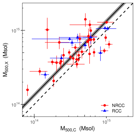
Figure 2: The hydrostatic versus the caustic masses are plotted for the full sample of clusters (with masses calculated at the hydrostatic $R_{500}$). NRCC clusters are red circles and RCC clusters are blue triangles. The solid black line shows the best fitting model to the full data, with the shaded region indicating the $1\sigma$ uncertainty. The 1:1 line is also plotted as a dashed black line.

The temperature profiles required for the hydrostatic mass estimates were measured out to radii close to, or beyond, $R_{500}$ for the majority of clusters (see Figure 10). For the mass profiles at radii greater than the extent of the temperature profile, we extrapolated the best fitting 3D temperature profile. As a consequence, our hydrostatic mass profiles beyond the extent of the measured temperature profiles are less robust. The median radius out to which the temperature profiles were measured is 0.95 $R_{500}$, and the range of radii is 0.51 - 1.62 $R_{500}$.

The use of the hydrostatic estimate of $R_{500}$ to determine both sets of masses introduces a covariance between the hydrostatic and caustic masses that is not included in our model. For this reason, we verified that using a fixed aperture of radius 1 Mpc for the mass measurements made a negligible difference to our results (as found in Maughan et al., 2016).

The $M_{X}/M_{C}$ profile of each cluster (calculated as $\hat{\mu_{X}}-\hat{\mu_{C}}$) is shown in Figure 3. We also plot the mean $M_{X}/M_{C}$ profile (calculated as the mean bias $\kappa$, see equation 7). The $M_{X}/M_{C}$ profile is consistent with the bias being constant with radius. At smaller radii the $M_{X}/M_{C}$ value decreases, but this is likely due to the caustic masses being overestimated at small radii (see e.g. Figure 12 Serra et al., 2011).

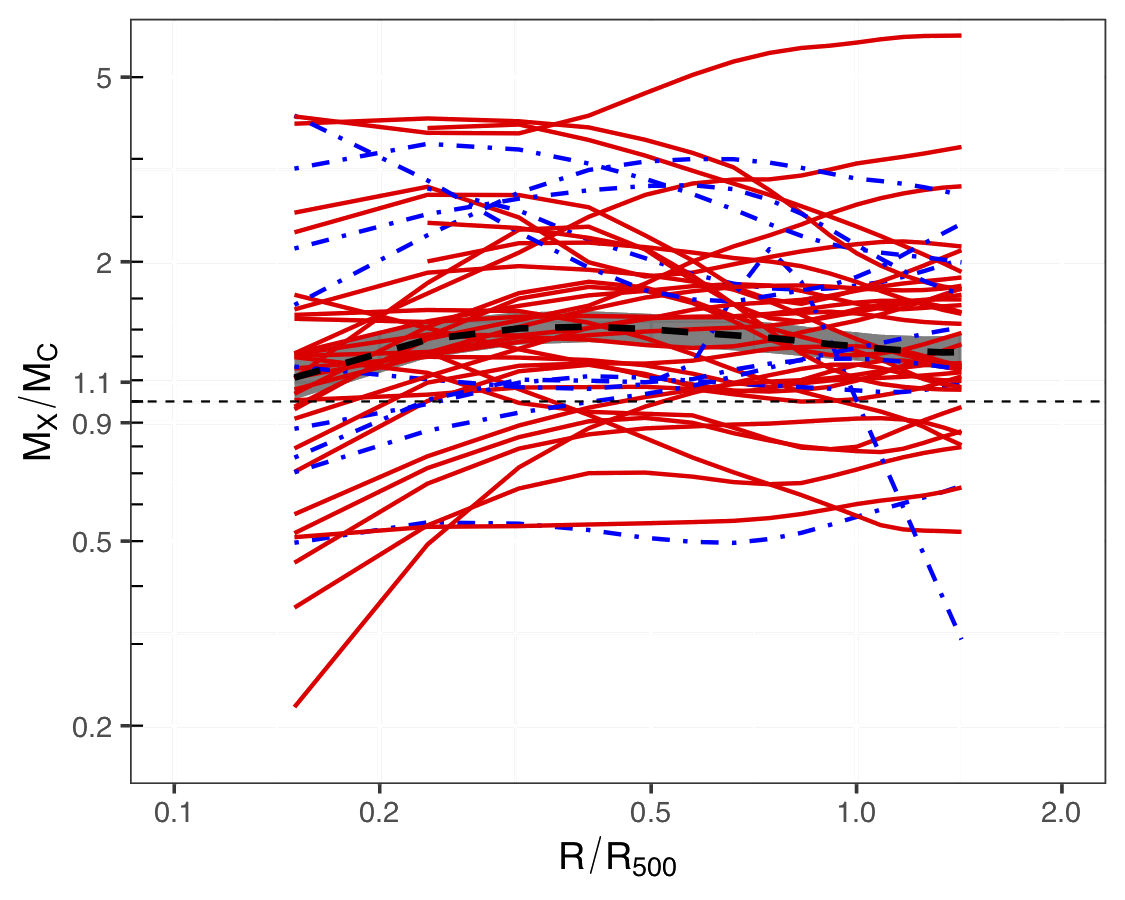
Figure 3: The $M_{X}/M_{C}$ profiles for all 44 clusters in our sample, scaled in radius by the hydrostatic $R_{500}$. NRCC clusters are solid red lines and RCC clusters are blue dot dashed lines. The 1:1 line is also plotted as a thin dashed black line. The thick dashed black line shows the average $M_{X}/M_{C}$ ratio, and the shaded region shows the 1$\sigma$ uncertainty.

The $M_{500,X}/M_{500,C}$ ratios at $R_{500}$ for the individual clusters is shown in Figure 4, and the average ratios are summarised in Table 4. At $R_{500}$ the caustic and hydrostatic masses generally do not agree well. For the full sample, the hydrostatic mass on average $\sim$ 30% higher than the caustic mass (significant at $\approx 3\sigma$). Similar results are found for both the NRCC and RCC clusters.

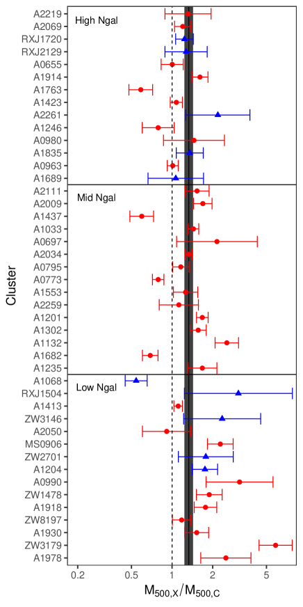
Figure 4: We show the $M_{500,X}/M_{500,C}$ ratio for all 44 clusters in our sample. NRCC clusters are red circles and RCC clusters are blue triangles. The solid black line and shaded region show the average $M_{500,X}/M_{500,C}$ ratio at the hydrostatic $R_{500}$. 1$\sigma$ errors are shown. The clusters are ranked by Ngal with the highest at the top, and the horizontal lines separate the clusters into the low, mid and high Ngal subsets (see §4.2).

This $M_{500,X}/M_{500,C}$ value is consistent with the our earlier findings (Maughan et al., 2016), but rules out $M_{500,X}/M_{500,C}=1$ at higher significance, and remains counter-intuitive. The hydrostatic mass is expected to be underestimated compared to the true mass (e.g. Nelson et al., 2014; Eckert et al., 2019) while the caustic mass expected to be overestimated compared to the true mass at $R_{500}$ (e.g. Serra et al., 2011); thus we expect the $M_{500,X}/M_{500,C}$ ratio to be less than 1.

Aperture	Subset	$N_{C}$	$\kappa$	$M_{500,X}/M_{500,C}$	$\delta$ (%)
$R_{500}$	All	44	0.123$\pm$0.031	$1.33^{+0.10}_{-0.09}$	$39^{+06}_{-06}$
$R_{500}$	RCC	10	0.126$\pm$0.102	$1.32^{+0.33}_{-0.24}$	$51^{+25}_{-16}$
$R_{500}$	NRCC	34	0.125$\pm$0.035	$1.33^{+0.11}_{-0.10}$	$41^{+07}_{-06}$

Table 4: Summary of the results from our mass comparison analysis. The first column gives the aperture within which the caustic and hydrostatic masses were calculated. For this column, $R_{500}$ refers to the hydrostatic $R_{500}$. The second column gives the subset for which the summary statistics are given, and the third column $N_{C}$ gives the number of clusters in that subset. Columns 4, 5 and 6 give the summary statistics. The mean bias is given in column 4, the median ratio of masses is given in column 5, and the intrinsic scatter between the caustic and hydrostatic mass is given in column 6. See §3.3 for details on how these values were derived.

4.2 Dependency on Ngal

Figure 2 suggests that the high value of the $M_{500,X}/M_{500,C}$ ratio for the full sample may be driven by clusters with lower caustic masses (with hydrostatic masses being overestimated and/or caustic masses being underestimated). However, simulations indicate that dynamical mass estimators in general (including a different implementation of the caustic method to that used here) tend to underestimate masses when the number of galaxies used is low (Wojtak et al., 2018). This is a confounding factor since the lower mass clusters tend to have lower Ngal.

In order to investigate the role of Ngal in our results, the sample was split on Ngal into three approximately equal subsets of 15, 15 and 14 clusters (see the Ngal sub-sample column in Table 3). These low, mid and high Ngal sub-samples have $63\leq\text{Ngal}\leq 129$ (mean 93), $131\leq\text{Ngal}\leq 208$ (mean 174), and $210\leq\text{Ngal}\leq 461$ (mean 281) respectively. Figure 5 shows the comparison between hydrostatic and caustic masses with the different Ngal subsets indicated. This illustrates the trend that lower mass clusters tend to have lower Ngal. It is also clear that, at a given hydrostatic mass, the clusters with the lowest Ngal are most discrepant in their caustic mass.

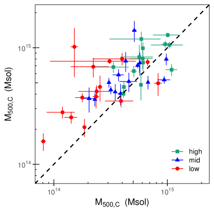
Figure 5: The hydrostatic and caustic masses measured within the hydrostatic $R_{500}$ are plotted for the full sample. This is the same data as plotted in Figure 2, but now showing the Ngal subsets. The high, mid and low Ngal bins are green squares, blue triangles and red circles respectively. The 1:1 line is also plotted as a dashed black line.

To investigate this further, the gas fraction, $f_{\text{gas}}$ (defined as the gas mass, $m_{\text{gas}}$, within some radius divided by the total mass within the same radius), was found to be a useful discriminator between possible systematics in the analysis. This is because $m_{\text{gas}}$ can be measured accurately from X-ray observations (e.g. Nagai et al., 2007), and there are robust theoretical predictions for the range of $f_{\text{gas}}$ expected. We thus computed $f_{\text{gas}}$ at a radius of 1 Mpc (chosen to avoid dependency of the radius on any mass estimation method) with either the hydrostatic and caustic masses in the denominator. The results are plotted in Figure 6. The plot also indicates the approximate range of $f_{\text{gas}}$ ($\sim$ 0.1 - 0.15) expected at this radius (e.g. Eckert et al., 2016).

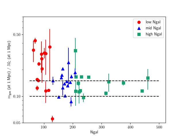
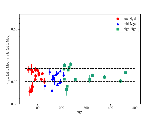
Figure 6: Left: $f_{\text{gas}}$ measured at 1 Mpc using caustic mass in the denominator is plotted against Ngal. Right: The same plot, but with $f_{\text{gas}}$ calculated with hydrostatic mass in the denominator. In both panels, the black dashed lines indicate $f_{\text{gas}}=0.10$ and $f_{\text{gas}}=0.15$ for reference, encompassing the approximate expected range of $f_{\text{gas}}$.

When the caustic mass is used as the denominator in $f_{\text{gas}}$, there is a strong indication of a trend with Ngal, with unphysically high values of $f_{\text{gas}}$ for the clusters with lower values of Ngal. The mean and standard error of $f_{\text{gas}}$ was 0.23$\pm$0.03, 0.15$\pm$0.01 and 0.15$\pm$0.01 for the low, mid and high Ngal sub-samples respectively.

In contrast, when the hydrostatic mass is used to compute $f_{\text{gas}}$, the trend with Ngal disappears, and the average values of 0.12$\pm$0.01, 0.11$\pm$0.01, 0.12$\pm$0.01, for the low, mid and high Ngal sub-samples respectively are consistent with the expected range.

These $f_{\text{gas}}$ measurements suggest that Ngal is responsible for the high values of $M_{500,X}/M_{500,C}$ due to an underestimate of $M_{C}$. However, due to the correlation between Ngal and mass, the possibility remains that a trend with mass is more fundamental. During the completion of the work presented here, additional caustic mass measurements became available in the HeCS-Omnibus catalogue (Sohn et al., 2020) that allow the effects of mass and Ngal to be separated. The new catalogue includes new caustic mass estimates for clusters in our sample, using the same caustic method, but based (in most cases) on a larger number of galaxies per cluster.

When comparing the earlier and newer caustic mass measurements, it was found that for well-sampled clusters, increasing the sampling had little effect on the mass. On the contrary, for more poorly sampled clusters, increasing Ngal systematically led to an increased mass estimate. This is illustrated in Fig. 7, which shows the ratio of the caustic masses (measured at the hydrostatic $R_{500}$) from Sohn et al. (2020) to those from both Rines et al. (2013) (as used in our work), plotted against the difference in Ngal between the two analyses.

The clusters were divided into subsets based on the minimum Ngal used in the two caustic calculations. For clusters where at least 200 galaxies were used in both analyses (green squares in Fig. 7), increasing the sampling has a weak or null effect on the mass estimate. The green line is a straight line fit to the data in this parameter space (i.e. $\log(M_{\text{Sohn}}/M_{\text{Rines}})$ versus $N_{\text{Sohn}}-N_{\text{Rines}}$) using BCES y on x regression (Akritas & Bershady, 1996). This is a simplistic model and is not intended to fully describe the systematic effects in the analyses, but is an adequate description of the data presented here. The slope of the line is $0.001\pm 0.001$.

The impact of increasing Ngal for less well-sampled clusters is seen in the blue triangles in Fig. 7. These are clusters for which Ngal is $<120$ in at least one of the two analyses. It is clear in the figure that increasing the sampling leads to systematically higher caustic mass estimates. The best fitting line to this subset has a slope of $0.008\pm 0.002$. The subsets were defined to split the sample into three equal groups, and the intermediate subset falls between the two outer cases and are omitted from the figure for clarity.

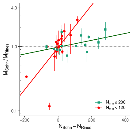
Figure 7: The ratio of the caustic masses (measured at the hydrostatic $R_{500}$) from Sohn et al. (2020) to those from Rines et al. (2013) are plotted as a function of the difference in Ngal between the analyses. The clusters are split into subsets containing those where the minimum Ngal used in the two analyses was at least 200 (green squares) and those where the minimum Ngal was less then 120 (red circles). The lines show the best fits to each subset.

We further test the role of Ngal as follows. We undersample the galaxy catalogues of the 14 clusters in our high-Ngal sub-sample, by progressively removing the faintest galaxies. When Ngal drops by $\sim 50\%$, falling in the range $\sim 100-200$, the caustic mass within $R_{500}$ decreases by $\sim 15\%$, on average. This average mass underestimate is consistent with the analysis of Serra et al (2011) who found that with $\text{Ngal}\sim 100$ the escape velocity at $R_{500}$ is underestimated by $\sim 5-10\%$, whereas $\text{Ngal}\gtrsim 200$ is required to return unbiased escape velocity estimates (see also Halenka et al., 2022). The lower Ngal of the undersampled clusters in our high-Ngal sample would move these clusters in our mid-Ngal sample: the $\sim 15\%$ mass underestimate we find in this test is thus also consistent with the larger ratio $M_{500,X}/M_{500,C}$ we find for our mid-Ngal sample, as illustrated in §4.3 below (Table 5).

Based on these results, we conclude that a systematic underestimate of the caustic mass at $R_{500}$ for low values of Ngal is responsible for the high apparent $M_{500,X}/M_{500,C}$ ratio found at low masses, and that the high Ngal sub-sample ($\text{Ngal}\geq 210$) is not significantly affected by this systematic. We thus repeat our analysis on the separate Ngal subsets in the following section, and will draw our final conclusions based on the results for the high Ngal subset alone.

4.3 Final results

The analysis described in §4.1 was repeated for each of the Ngal subsets separately, and the results are summarised in Table 5. Figure 8 shows the profiles of $M_{X}/M_{C}$ for the different Ngal subsets. The separation between the subsets is clear, with no radial dependency.

Aperture	Subset	$N_{C}$	$\kappa$	$M_{500,X}/M_{500,C}$	$\delta$ (%)
$\mathbf{R_{500}}$	High	14	$\mathbf{0.050\pm 0.043}$	$\mathbf{1.12^{+0.11}_{-0.10}}$	$\mathbf{25^{+12}_{-08}}$
$R_{500}$	Mid	15	0.109$\pm$0.053	$1.28^{+0.16}_{-0.14}$	$41^{+12}_{-09}$
$R_{500}$	Low	15	0.230$\pm$0.082	$1.69^{+0.33}_{-0.27}$	$59^{+18}_{-13}$

Table 5: Summary of the results from our mass comparison analysis when we define subsets of our clusters based on the Ngal value. The columns are the same as in Table 4. The line in bold represents the most reliable results, based on the high Ngal subset.

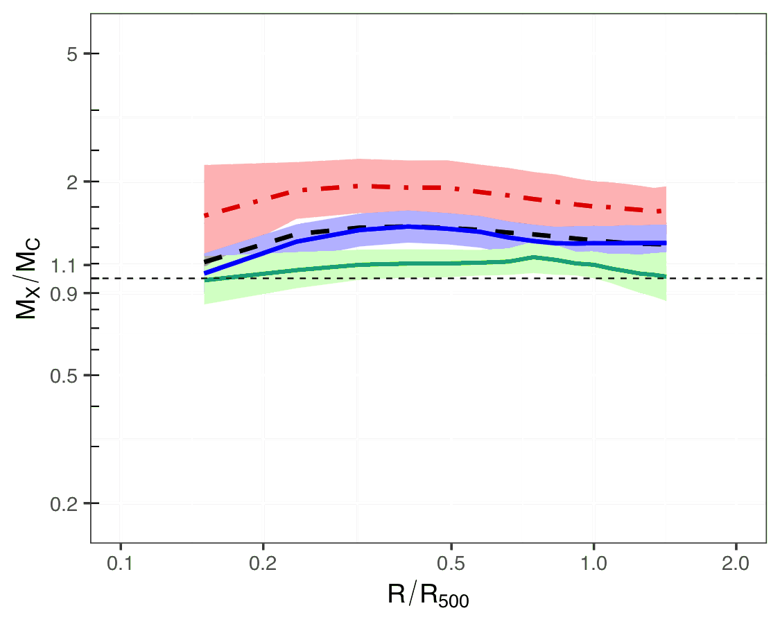
Figure 8: The average $M_{X}/M_{C}$ profiles for the high Ngal, mid Ngal and low Ngal clusters in green lines, blue lines, and red dot-dashed lines respectively. The 1:1 line is also plotted as a thin black dashed line. The thick dashed black line shows the average $M_{X}/M_{C}$ profile for all clusters. The profiles are scaled in radius by the hydrostatic $R_{500}$, and the shaded regions show the 1$\sigma$ uncertainties.

As expected based on the preceding analysis, the results in Table 5 show a trend towards lower $M_{X}$/$M_{C}$ ratios with increasing Ngal. The most reliable results are those based on the sample of 14 clusters with the highest values of Ngal, and these are highlighted in boldface in the table. For this subset, the average ratio of hydrostatic to caustic masses is $M_{500,X}/M_{500,C}=1.12^{+0.11}_{-0.10}$ with an intrinsic scatter between the masses of $\delta=(25^{+12}_{-08})\%$.

The comparison between the hydrostatic and caustic masses for the high Ngal subset is shown in Figure 9, with the RCC/NRCC classification of the clusters indicated. There does not appear to be a significant trend with dynamical state but given the reduced size of this high Ngal subset, a more detailed analysis would not be useful.

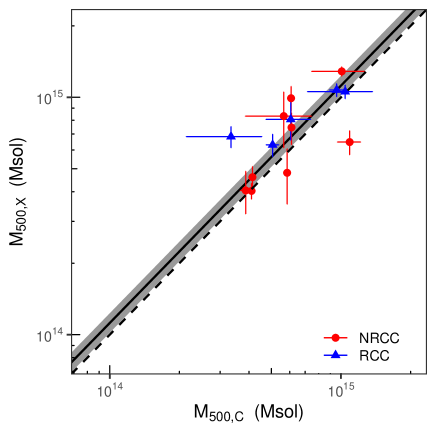
Figure 9: We show the hydrostatic masses versus the caustic masses for the 14 clusters in our sample with the highest Ngal values, both calculated at the hydrostatic $R_{500}$. We show RCC clusters as blue triangles and NRCC clusters as red circles. The solid black line shows the best fitting model, with the shaded region indicating the $1\sigma$ uncertainty. The 1:1 line is also plotted as a dashed black line.

Recall that 14 of the 16 clusters used in our earlier analysis in Maughan et al. (2016) are in common with the current analysis. Of these, six are in our high Ngal subset, seven are in the mid Ngal sub-sample, and one is in the low Ngal sub-sample. This mix of mid- and high-Ngal clusters naturally explains why Maughan et al. (2016) found an $M_{X}$/$M_{C}$ ratio that was slightly higher ($M_{500,X}/M_{500,C}=1.20\pm 0.12$) than our final result for the high Ngal subset.

5 Discussion

In the following section we consider the possible systematics that could have impacted our results. We explore in more detail our conclusion that the apparent increase in $M_{500,X}/M_{500,C}$ at low masses is driven by Ngal rather than by mass (or some other factor). Finally, we compare our results with other related analyses, and discuss the constraints that can be derived on the level of hydrostatic bias in massive clusters.

5.1 The impact of Ngal

Our investigation of the comparison between hydrostatic and caustic masses suggested that the caustic masses were underestimated when fewer galaxies were used. While a general result of dynamical masses being biased low when based on smaller numbers of galaxies was shown in Wojtak et al. (2018), the caustic method examined in that work differed from the implementation used here.

The dependence on Ngal of the caustic mass was investigated for our implementation of the caustic method by Serra et al. (2011). They found that the true escape velocity profile will be underestimated by $\sim$5-10% at $R_{500}$ (Figure 20, Serra et al., 2011) for clusters with Ngal $\sim$ 100 (compared to clusters with a higher Ngal for which the true escape velocity is not underestimated). This would lead to the caustic mass being underestimated by $\sim$10-20% at $R_{500}$, were it not for the assumption of a constant $\mathcal{F}_{\beta}$ (see §3.2), which leads to a $\sim$10-15% overestimate of the true mass at $R_{500}$ for clusters with a higher Ngal (Figure 12, Serra et al., 2011). Thus, the simulations suggest that these two effects approximately cancel out at our comparison radius of $R_{500}$, such that a large underestimation of the cluster mass using the caustic method for low Ngal clusters (like that implied by our results) is not expected.

As discussed in §4.2, we consider the caustic masses for the high Ngal subset to be unaffected by this apparent bias, and base our main conclusions on this subset. As a test of the robustness of our results, we repeated the measurement of $M_{500,X}/M_{500,C}$ using the HeCS-Omnibus caustic data of Sohn et al. (2020) in place of the original HeCS caustic data of Rines et al. (2013) that was used for our main analysis. We selected the 14 clusters in our sample with the highest Ngal in HeCS-Omnibus ($\text{Ngal}>274$ with a median of $413$). For these best-sampled clusters, using the HeCS-Omnibus caustic masses gives an average hydrostatic to caustic mass ratio of $M_{500,X}/M_{500,C}=1.10$ at the hydrostatic $R_{500}$. This agrees very well with the $M_{500,X}/M_{500,C}=1.12$ we found for the 14 clusters in our high Ngal subset when using the Rines et al. (2013) data (for which $\text{Ngal}>210$ with a median of 234). This supports our conclusion that our high Ngal subset is unaffected by systematics due to low numbers of galaxies (i.e. $\text{Ngal}\,\hbox to0.0pt{\raise 1.72218pt\hbox{$>$}\hss}{\lower 2.58334pt\hbox{$\sim$}}\,200$ is sufficient to avoid biases in the caustic mass at $R_{500}$). Indeed, when we apply the caustic technique to the cluster catalogues in the high-Ngal sample where we undersampled Ngal such that $\text{Ngal}\lesssim 200$, the caustic mass within $R_{500}$ is underestimated by $\sim 15\%$, on average, suggesting that the increase of the ratio $M_{500,X}/M_{500,C}$ from $\sim 1.12$ of the high-Ngal sample to $\sim 1.28$ of the mid-Ngal sample is mostly driven by the lower number of the caustic members.

Poorer sampling of the caustics is likely to be responsible (at least in part) for some of the outliers seen in the comparisons between the hydrostatic and caustic masses (e.g in Figure 4). When restricted to the high Ngal subset, there are no significant outliers in the comparison between hydrostatic and caustic masses, given the $\sim 30\%$ intrinsic scatter between the mass estimators (e.g. Figure 9).

5.2 Cluster centres and apertures

In the caustic analysis, the cluster centre is located as part of the process (Rines et al., 2013), while the centre is fixed at the X-ray centroid for the hydrostatic analysis. This means that the profiles are not generally centred at the same location. The separation between the centres used for the X-ray and caustic analyses were generally small, and showed no trend with Ngal or with $M_{500,X}/M_{500,C}$ (the median separation was $\approx 130\mbox{$\text{\leavevmode\nobreak\ kpc}$}$ in each of the Ngal subsets). We thus conclude that the increasing disagreement between hydrostatic and caustic masses at low Ngal is not being driven by miscentring.

Serra et al. (2011) investigated the impact of miscentering of the caustic analyses on the mass determination in their simulations. At $R_{500}$, the caustic mass estimate was increased by $\approx 10\%$ when the profile was forced to use the true centre. This suggests that our measurements of $M_{500,X}/M_{500,C}$ could be overestimated by $\approx 0.1$ due to miscentring of the profiles.

When the separation between the centres used for the caustic and hydrostatic analyses is small, then the use of a common aperture size (i.e. the hydrostatic $R_{\text{500}}$) allows the mass estimators to be compared without adding scatter from different aperture definitions. However, given that the centres are not identical, it is also helpful to compare the masses when they are derived fully independently (i.e. comparing the caustic mass within the caustic $R_{\text{500}}$ with the hydrostatic mass within the hydrostatic $R_{\text{500}}$).

We repeated our analysis using these independent definitions of $R_{\text{500}}$. For the full sample of 44 clusters, we found that mass ratio increased from $M_{500,X}/M_{500,C}=1.33^{+0.10}_{-0.09}$ (using the hydrostatic $R_{\text{500}}$) to $M_{500,X}/M_{500,C}=1.52^{+0.16}_{-0.14}$ (using independent $R_{\text{500}}$). In the case of the high Ngal sub-sample, the original $M_{500,X}/M_{500,C}=1.12^{+0.11}_{-0.10}$ (hydrostatic $R_{\text{500}}$) increased slightly to $M_{500,X}/M_{500,C}=1.16^{+0.16}_{-0.13}$ (independent $R_{\text{500}}$).

These results make sense. When the masses agree well (as in the high Ngal sub-sample) then the $R_{\text{500}}$ definitions also agree so the results do not change. If the masses are more discrepant (as in the full sample) then using the independent $R_{\text{500}}$ will tend to amplify the difference.

As might be expected, the scatter between the mass estimators is somewhat larger when the independent $R_{\text{500}}$ are used. The scatter increases from $(39\pm 6)\%$ to $(55^{+9}_{-8})\%$ for the full sample, and from $(25^{+12}_{-08})\%$ to $(35^{+15}_{-11})\%$ for the high Ngal sub-sample.

Based on this analysis, we conclude that the use of the hydrostatic $R_{\text{500}}$ for both mass determinations does not have a strong effect on our results.

5.3 Impact of selection effects

In our work we do not account for the impact of selection effects in our model. The sample is selected on the basis of X-ray flux, so covariance between X-ray flux and $M_{X}$ could have an impact on the inferred $M_{500,X}/M_{500,C}$ ratio. Specifically, if there were a strong positive covariance between X-ray luminosity, $L_{X}$, and hydrostatic mass, $M_{X}$, given the true mass, then X-ray selection would select clusters that were both more luminous than average and had higher hydrostatic masses than average, given their true mass. The size of this effect would depend both on the scatter in the relevant relations and the degree of covariance between $M_{X}$ and $L_{X}$.

We assessed the possible impact of this selection effect by simulating cluster populations with different degrees of covariance between $L_{X}$ and $M_{X}$, imposing the sample selection function, and then applying our model (described in §3.3) to the simulated population to determine the impact of the sample selection on the recovered $M_{500,X}/M_{500,C}$ ratio.

In more detail, we sampled a large number of points from a mass function where each point consists of a true mass, $M_{\text{true}}$, and a redshift. We use the mass - luminosity relation from Mantz et al. (2010) to assign the true luminosity, $L_{\text{true}}$ to each cluster. We then assume a scatter between $L_{\text{true}}$ and $L_{X}$ of 30%, a scatter between $M_{\text{true}}$ and $M_{X}$ of 10% and a scatter between $M_{\text{true}}$ and $M_{C}$ of 30%. We also require a correlation coefficient, $\rho_{LM}$, between $L_{X}$ and $M_{X}$ to create the covariance matrix for the multi-dimensional Gaussian from which we sample $L_{X}$ and $M_{X}$ from $L_{\text{true}}$ and $M_{\text{true}}$. It is the strength of this correlation coefficient that dictates how much a selection on X-ray flux might bias an inference based on hydrostatic masses, and we investigate the impact of different assumed values below. Finally, we apply our X-ray selection to the fluxes derived from the $L_{\text{true}}$ and redshift values, and use our model to measure the $M_{500,X}/M_{500,C}$ ratio for the resulting simulated sample. We do not set any hydrostatic or caustic bias in the simulation, so in the absence of selection biases, we would measure $M_{500,X}/M_{500,C}=1$.

To our knowledge, covariances between $L_{X}$ and hydrostatic mass have not been measured in the literature, but the covariances between other ICM properties have been investigated in a few studies (e.g. Maughan, 2014; Mantz et al., 2016; Andreon et al., 2017b; Farahi et al., 2018). For example, for the covariance between $L_{X}$ and $m_{\text{gas}}$, Mantz et al. (2016) found a correlation coefficient of 0.43, while Farahi et al. (2018) found 0.76. Meanwhile, for the covariance between $L_{X}$ and $T$, Mantz et al. (2016) found a correlation coefficient of 0.53, while Farahi et al. (2018) found 0.49. In both cases, the values obtained by Mantz et al. (2016) are the more relevant here since they make use of a soft-band, core-included X-ray luminosity, which matches the selection method used for our sample (Farahi et al., 2018, made use of bolometric luminosities with the core regions removed, but we include their results here for comparison). We therefore conclude that a correlation coefficient of $\rho_{LM}=0.5$ is a reasonable upper limit on the strength of the covariance between $L_{X}$ and $M_{X}$ and use this as a reference value for our simulations. We also performed the simulations with with $\rho_{LM}=1$ as a maximally pessimistic case.

We find that for $\rho_{LM}=0.5$, the recovered $M_{500,X}/M_{500,C}$ value is 1.03$\pm$0.01 and for $\rho_{LM}=1$ we measured $M_{500,X}/M_{500,C}=1.07\pm 0.01$ (for a sample of 500 simulated clusters).

We also checked for a mass dependence of the selection bias by splitting the simulated clusters into low (log($M_{X}$)¡14.5), mid (14.5¡log($M_{X}$)¡14.75), and high (log($M_{X}$)¿14.75) mass sub-samples (each containing 500 simulated clusters). The measured $M_{500,X}/M_{500,C}$ ratio was largest for the low-mass sub-sample, due to a larger proportion of the clusters being close to the flux limit. For the low-mass sub-sample, assuming $\rho_{LM}=0.5$ we found $M_{X}/M_{X}=1.06\pm 0.01$, increasing to $1.15\pm 0.01$ for $\rho_{LM}=1$. For the high mass sub-sample (which is similar in mass to our high Ngal subset), the measured $M_{500,X}/M_{500,C}$ ratios dropped to 1.02$\pm$0.01 and 1.03$\pm$0.01 for $\rho_{LM}=0.5$ and $\rho_{LM}=1$ respectively.

We conclude that, while neglecting selection effects tends to bias the $M_{500,X}/M_{500,C}$ ratio high, the impact is not significant for the mass range of the high Ngal subset, and that selection biases alone cannot explain the high values of $M_{500,X}/M_{500,C}$ that we find in the lower mass, lower Ngal clusters.

5.4 Impact of X-ray temperature calibration

It is established that there are systematic differences in cluster temperatures measured by Chandra and XMM-Newton, temperatures measured with Chandra being systematically hotter (Schellenberger et al., 2015). This has been found to have a corresponding systematic impact on the derived hydrostatic masses Mahdavi et al., 2013; Schellenberger et al., 2015). We note, however, that Martino et al. (2014) found no systematic differences in hydrostatic masses for a sample of 50 clusters with both XMM-Newton and Chandra data.

Schellenberger et al. (2015) found that the hydrostatic masses measured from Chandra data were $14\pm 2\%$ higher than those from XMM-Newton. They found no significant trend with cluster mass, suggesting that the apparent trend of $M_{500,X}/M_{500,C}$ with mass or Ngal that we find is not driven by this systematic. If our hydrostatic masses were systematically overestimated by $\approx 15\%$, this would have a direct effect of reducing our derived $M_{500,X}/M_{500,C}$ ratios by $0.15$.

5.5 Summary of systematics

We have identified a number of possible systematics that could impact our comparison between caustic and hydrostatic masses. In the case of the caustic masses, poorer sampling of the caustics was found to result in an underestimate of the caustic masses for $\text{Ngal}\la 200$, producing an apparent trend of $M_{500,X}/M_{500,C}$ with mass. For the better-sampled clusters, this systematic appears to be absent, but the assumption of constant $\mathcal{F}_{\beta}$ is expected to lead to an overestimate of the caustic mass by $10-15\%$ at $R_{500}$ (i.e. biasing $M_{500,X}/M_{500,C}$ low by up to $0.15$). The miscentering of the caustic profiles leads to an estimated underestimate of the caustic masses of $\approx 10\%$ at $R_{500}$ (biasing $M_{500,X}/M_{500,C}$ high by $\approx 0.1$).

We find that the use of X-ray flux to select the sample combined with a possible covariance between X-ray luminosity and hydrostatic mass could bias the hydrostatic masses to be high. However, the effect is estimated at a few percent for the more massive clusters comprising our high Ngal subset, and the trend with mass is not sufficient to explain the strength of the trend of $M_{500,X}/M_{500,C}$ with mass or Ngal. Finally, systematics on the calibration of Chandra could lead to the hydrostatic masses being overestimated by $\approx 15\%$ (biasing $M_{500,X}/M_{500,C}$ high by about $0.15$).

5.6 Comparison with other work

Direct comparisons between hydrostatic and caustic masses for samples of clusters are scarce in the literature. Andreon et al. (2017a) compared the mean $f_{gas}$ for a sample of 34 clusters with caustic masses, with the mean value from separate samples with hydrostatic masses from Chandra data. They inferred that caustic masses were slightly higher than, but consistent with, hydrostatic masses at $R_{500}$. This is consistent with the result we find for the high Ngal subset. However, the clusters with caustic masses used in Andreon et al. (2017a) cover a range in mass and Ngal that is comparable with our low and mid Ngal subsets, and are in tension (at the $\approx 2\sigma$ level) with those subsets for which we find the caustic masses to be lower than hydrostatic masses (although we consider our results for those subsets to be less reliable due to the poorer sampling of the caustics).

Foëx et al. (2017) compared hydrostatic and caustic masses for a sample of 13 clusters with masses, redshifts and Ngal similar to our high Ngal subset. They found a mean $M_{C}/M_{X}=1.32\pm 0.18$ at $R_{500}$ (we note that this is the inverse of our mass ratio), and hence caustic masses were higher than hydrostatic masses by $\sim 30\%$ (although the ratio dropped to unity when some substructures were removed in the dynamical analysis). While this contrasts with our results, the difference is not strongly significant ($\approx 2\sigma$). Furthermore, the Foëx et al. (2017) analysis was based on hydrostatic masses from XMM-Newton; adjusting these masses to match the Chandra calibration would reduce the tension with our result to less than $1\sigma$.

Ettori et al. (2019) compared hydrostatic masses (from XMM-Newton) and caustic masses at $R_{200}$ for 6 clusters, finding that the caustic masses were lower than the hydrostatic masses by about $30\%$ on average. This is in the same sense as the difference we find for our sample, but the clusters include some with lower Ngal than our high Ngal subset, so a direct comparison is not possible.

5.7 Implications for the hydrostatic bias

Conventionally, the hydrostatic bias is defined as $b=1-M_{X}/M$, where $M_{X}$ is the hydrostatic mass and $M$ is the true mass. Our best estimate of the ratio of hydrostatic to caustic masses, with statistical error is $M_{500,X}/M_{500,C}=1.12^{+0.11}_{-0.10}$, for the high Ngal subset. Under the strong assumption that the caustic masses are unbiased, we can write $b=1-M_{500,X}/M_{500,C}$, in which case our results exclude a hydrostatic bias of more than $20\%$ at the $3\sigma$ level based on statistical uncertainty alone. However, taking the possible systematic uncertainties on both the caustic and hydrostatic masses into account, we cannot rule out larger values of the hydrostatic bias.

Constraints on the hydrostatic bias from direct comparisons between hydrostatic and WL masses currently encompass a range from approximately zero (e.g. Gruen et al., 2014; Israel et al., 2014; Applegate et al., 2016; Smith et al., 2016) up to around $30\%$ (e.g von der Linden et al., 2014; Donahue et al., 2014; Hoekstra et al., 2015). Meanwhile, constraints on the level of bias have also been estimated indirectly by comparisons of WL masses with masses derived from scaling relations of other observables that were calibrated to hydrostatic masses (e.g. from X-ray luminosity Sereno & Ettori (2017) or the Sunyaev-Zel’dovich effect signals Medezinski et al. (2018); Miyatake et al. (2019)). These also tend to favour biases of $20-30\%$.

The question of hydrostatic bias has also been addressed with simulations, which typically find biases of $10-30\%$, but with radial and mass dependences, and sensitivity to the method used to reconstruct the hydrostatic masses from the simulation data (e.g. Nagai et al., 2007; Rasia et al., 2012; Pearce et al., 2020; Barnes et al., 2021).

Simulations suggest a significant mass dependence of the hydrostatic bias, with the bias increasing for higher mass clusters (e.g Barnes et al., 2021). However, due to the relatively poorer sampling of the caustics in our lower mass clusters, we are not able to test these results observationally.

Overall, there is not a clear consensus on the magnitude of the hydrostatic bias. Our results are more consistent with those estimates from the low end of the range and add a useful new datapoint to this still-open question, since the caustic mass determination is subject to different systematics and assumptions to those affecting the WL masses which are primarily used to address this question observationally.

6 Summary and conclusions

We compared masses of 44 galaxy clusters determined independently from X-ray data under the assumption of hydrostatic equilibrium, and galaxy velocities using the caustic method. Our initial results showed significant discrepancies between the masses which appeared to increase for lower mass clusters. We found that this was driven by the poorer sampling of the caustics for the lower mass clusters leading to an underestimate of the mass using the caustic method at $R_{500}$. The caustic method is not optimised for mass determinations at these radii, but this finding suggests that simulations have underestimated the impact of poorer sampling at smaller radii.

Restricting our analysis to the 14 clusters with best-sampled caustics (the high Ngal subset), we find an average ratio of the hydrostatic to caustic masses of $M_{500,X}/M_{500,C}=1.12^{+0.11}_{-0.10}$. We find no evidence for radial dependence of this ratio or dependence on dynamical state of the cluster, but these conclusions are limited by the reduced sample size.

We investigated possible systematics that could affect the mass estimates for this high Ngal subset and find that the most significant are as follows. The assumption of constant $\mathcal{F}_{\beta}$ and possible miscentering of the caustic profiles could bias the caustic masses high and low respectively by $10-15\%$. The uncertainties on the absolute calibration of the X-ray temperature measurements could bias the hydrostatic masses high by about $15\%$ compared to those measured with XMM-Newton.

We interpret our results as favouring a hydrostatic bias that is close to zero. However, the systematics we identified would allow for significantly larger levels of hydrostatic bias.

Appendix A Notes on individual clusters

In this section we detail where we differed from the analysis methods presented in §3, or any particular points of interest for each cluster in our sample.

When extended sources other than the cluster were detected in the images, we attempted to determine if they were physically associated with the cluster or were unrelated projected sources. We did this by querying the NASA Extragalactic Database to see if the source has a known counterpart.

• A773 - For ObsID 5006, due to flaring we only use the first 15 ks of the observation.

• MS0906 - At 9:08:58.02, 11:01:58.36 (RA, DEC = 137.24, 11.03), there is a large region of diffuse extended emission (which corresponds to cluster A750 (Abell et al., 1989)) which we mask with a 230^′′ radius circle.

• ZW2701 - At 9:53:05.85, 51:49:16.39 (148.27, 51.82) there is a region of extended emission that we mask with a 150^′′ radius circle.

• A963 - For ObsID 903, a temperature of 0.28 keV was used when fitting the APEC model to the soft background residuals. We note that the standard temperature used for this is 0.18 keV, as it is found that this temperature generally models these residuals well (Giles et al., 2015). The higher temperature implies that this observation includes a hotter region of the galactic foreground emission.

• ZW3146 - For ObsID 9371, due to flaring we only use the first 34 ks of the observation.

• A1423 - For ObsID 538, due to flaring we only use the first 11 ks of the observation.

• A1553 - For ObsID 12254, due to flaring we only use the first 10 ks of the observation.

• A1682 - At 13:06:59.904, 46:31:40.65 (196.75, 46.53) there is a cluster galaxy (Morrison et al., 2003) and at 13:07:13.47, 46:29:02.31 (196.81, 46.48) there is another small region of extended emission. Both sources are masked by radius 40^′′ circles.

• A1763 - At 13:34:52.8, 40:57:21.6 (203.72, 40.96) we use a 90^′′ radius circle to mask a region of extended emission, which is likely to be associated with a previously known X-ray source (Evans et al., 2010).

• A1930 - At 14:32:42.72, 31:33:50.4 (218.18, 31.56) there is a region of extended emission that we mask with a circle of radius 160^′′. The extended emission is the cluster RM J143242.6+313407.1 (Rozo et al., 2015) at redshift $z=0.137$, and is likely part of the same dark matter halo as A1930 (z = 0.1308).

• A2009 - For ObsID 10438, a temperature of 0.27 keV was used when fitting the APEC model to the soft background residuals.

• A2069 - There is a separate cluster at 15:24:25.846, +30:00:16.039 (231.11, 30.00) at redshift $z=0.119$ (MaxBCG J231.10029+30.00604, Koester et al., 2007); it is likely part of the same dark matter halo as A2069. We mask it with a rectangle of 23^′ by 14^′ at an inclination angle of 35^∘. There is either a group of point sources or a filament at 15:23:38.87, +29:58:30.226 (230.91, 29.98) that we mask using an ellipse. In addition, for ObsID 4965, due to flaring we only use the first 40 ks of the observation.

• A2261 - At 17:22:12.78, 32:06:36.95 (260.55, 32.11) there is a region of diffuse extended emission that we mask with a 80^′′ radius circle. This source is associated with a galaxy cluster (GMBCG J260.55436+32.11438) at $z=0.304$ (Hao et al., 2010), so is not associated with A2261 which is at redshift $z=0.2242$.

• RXJ1720 - For ObsID 4361, due to flaring we only use the first 15 ks of the observation.

Appendix B Temperature and density profiles

In this Appendix we expand on the method used to model the temperature and density profiles used to determine the hydrostatic masses in §3.

B.1 Temperature Profiles

The model used for the 3D distribution of the temperature (Vikhlinin et al., 2006) is sufficient to describe a temperature decline (if present) in the central core region of the cluster in addition to the rest of the cluster temperature profile outside the central cooling region of a cluster. The part outside the central cooling region is modelled by

$$t(r)=-\frac{(r/r_{t})^{-a}}{\left[1+(r/r_{t})^{b}\right]^{c/b}}\quad,$$ (8)

where $r$ is the radius of the cluster and all other symbols are free parameters: $a$ models the slope at small radii, $c$ models the slope at large radii, and $b$ models the width of the transition between these slopes. This transition occurs at a radius $r_{t}$. The decrease in temperature found in the central cooling region of many clusters can be modelled as

$$t_{cool}(r)=-\frac{(x+T_{min}/T_{0})}{x+1}\quad,\qquad x=\left(\frac{r}{r_{cool}}\right)^{a_{cool}},$$ (9)

where $r$ is cluster radius and all other symbols are free parameters: $T_{0}$ is the normalisation, $T_{min}$ is the minimum temperature, $r_{cool}$ models radius of the central cooling region and $a_{cool}$ models the slope of the cool region which extends to a radius $r_{cool}$.

The 3D temperature profile model is a product of equations 8 and 9

$$T_{3D}(r)=T_{0}\,t_{cool}(r)t(r)\quad.$$ (10)

B.2 ICM density profiles

The model used to describe the 3D distribution of the density (Vikhlinin et al., 2006) is given by:

$$n_{\text{e}}n_{\text{p}}=n_{0}^{2}\frac{(r/r_{c})^{-\alpha}}{(1+r^{2}/r_{c}^{2})^{3\beta-\alpha/2}}\frac{1}{(1+r^{\gamma}/r_{s})^{\epsilon/\gamma}}+\frac{n_{02}^{2}}{(1+r^{2}/r_{c2}^{2})^{3\beta_{2}}},$$ (11)

with $r$ being the cluster radius and the nine free parameters able to model both the central and outer parts of the density profile sufficiently. We fix $\gamma=3$ as in Vikhlinin et al. (2006), and all the other parameters are free. $n_{\text{e}}$ and $n_{\text{p}}$ are the electron and proton density respectively, and $r$ is the distance from the centre of the cluster. The first term in the equation is a modification of the $\beta$-model (Cavaliere & Fusco-Femiano, 1978) that allows for a power-law type cusp, with slope $\alpha$ at small radii, which is expected in the centres of clusters that are dynamically relaxed. The second term models the change of the slope by $\epsilon$ near the radius $r_{s}$, and the width of this transition region is controlled by $\gamma$. The final term is another $\beta$-model component, which increases the freedom of the overall model near the cluster centre.

B.3 Projection of 3D profiles

The 3D temperature and density profiles must be projected before they can be compared with the observed profiles. For this projection we assume spherical symmetry (see e.g. Ettori et al., 2013, for the geometry of this projection). We note that whenever we use an abundance profile in our analysis, we use the measured projected abundance profile (we lack the very high quality data needed to deproject abundance profiles), and at large radii set the abundance to 0.3 $Z_{\odot}$, in line with observed flattening of abundance profiles at large radii (Leccardi & Molendi, 2008).

The projected temperature profile was computed using the method described in Vikhlinin et al. (2006). Briefly, the temperature that would be measured when fitting a single temperature thermal plasma model to the projected emission is computed by weighting the different temperature components of the 3D model along the line of sight by their emissivity. The emissivity is derived from the projected abundance and 3D density model, and the weighting algorithm of Vikhlinin (2006) was used.

The 3D density profile is projected to produce a model surface brightness profile. The count rate from each volume element along the line of sight is computed assuming an APEC plasma emission model with the normalisation set by the density in the volume element, and the temperature given by the 3D temperature profile model. This conversion from 3D density to projected surface brightness uses the appropriate instrument response for the detector location.

In the fitting process, the projection of the temperature and density profiles are performed simultaneously for a given set of model parameters to produce projected temperature and surface brightness profiles that are compared with the data. This is an improvement over the method used in Maughan et al. (2016), where a normalised average temperature profile was assumed when converting from density to emissivity.

Appendix C Mass profile plots

Figure 10 shows the X-ray hydrostatic and caustic mass profiles for the 44 clusters in our sample.

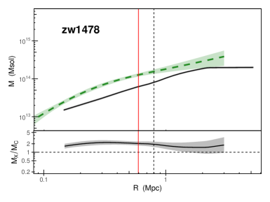
(a)

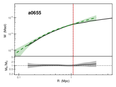
(b)

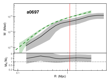
(c)

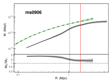
(d)

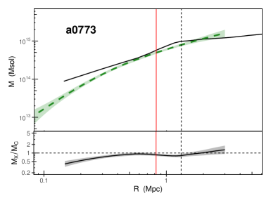
(e)

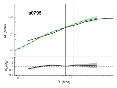
(f)

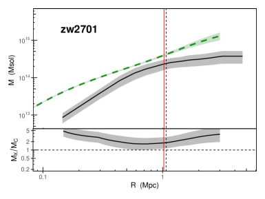
(g)

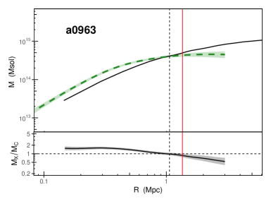
(h)

Figure 10: The caustic and hydrostatic mass profiles for each cluster as black solid and green dashed lines respectively in the upper panels of each plot. The ratio of the hydrostatic to caustic mass, $M_{X}/M_{C}$, are shown in the lower panels of each plot. 1$\sigma$ uncertainties are shown by the shaded regions. The vertical black line is at the value of $R_{500}$ as calculated from the hydrostatic mass profile; the solid red vertical line is at the outer radius of the measured temperature profile (note that hydrostatic masses beyond this radius are based on extrapolation).

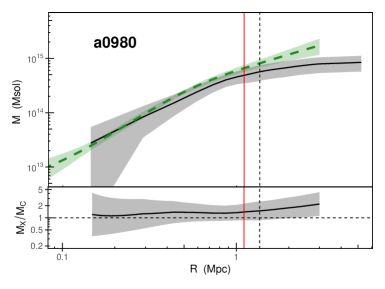
(i)

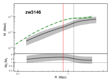
(j)

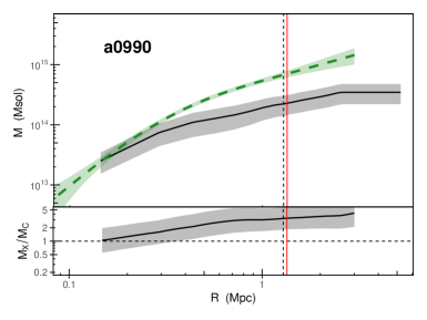
(k)

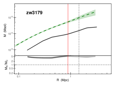
(l)

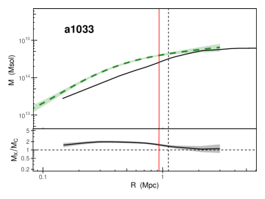
(m)

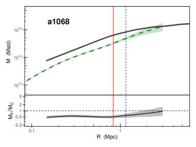
(n)

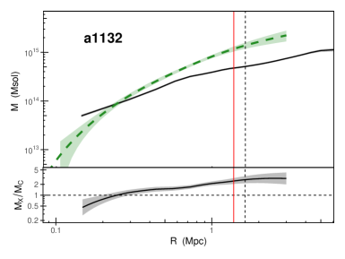
(o)

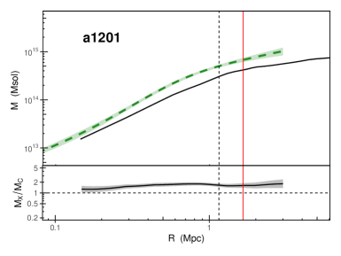
(p)

Figure 10: - continued

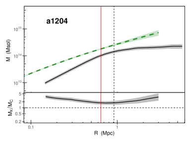
(q)

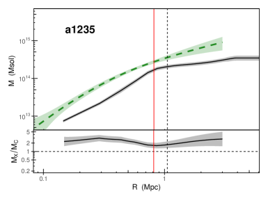
(r)

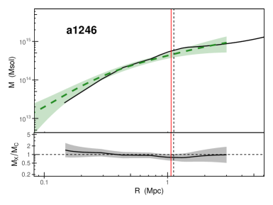
(s)

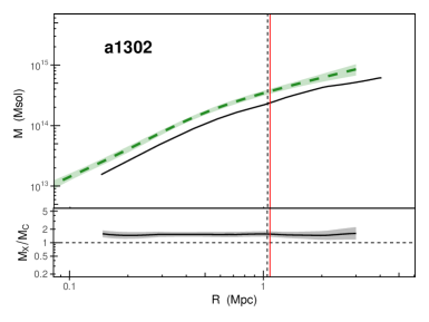
(t)

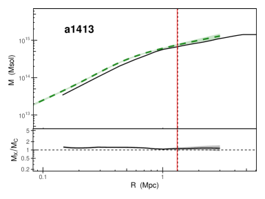
(u)

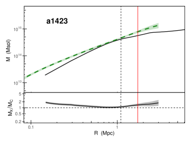
(v)

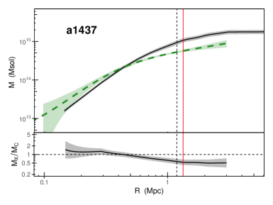
(w)

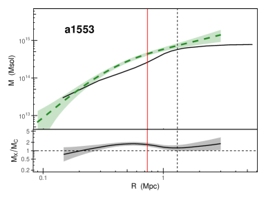
(x)

Figure 10: - continued

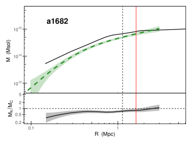
(y)

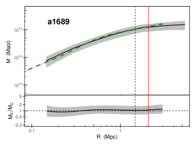
(z)

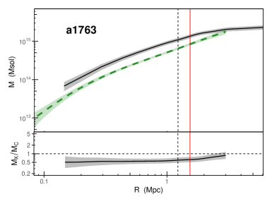
(aa)

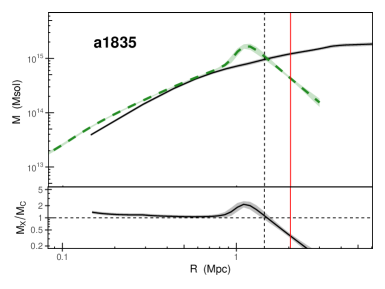
(ab)

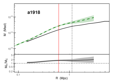
(ac)

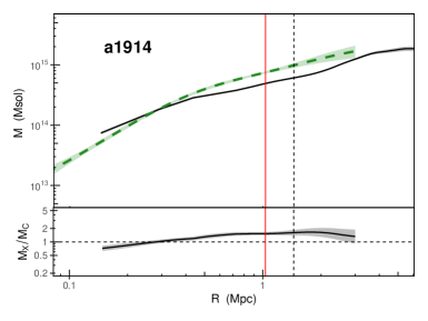
(ad)

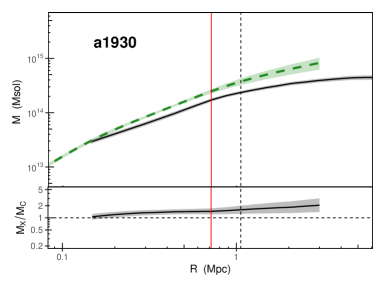
(ae)

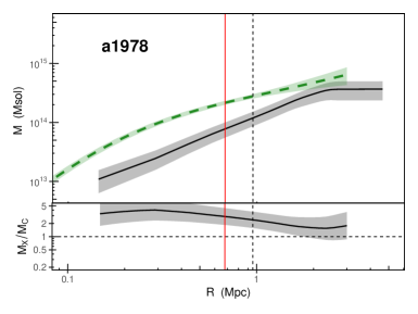
(af)

Figure 10: - continued

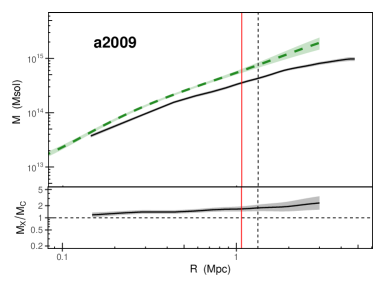
(ag)

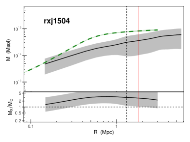
(ah)

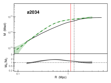
(ai)

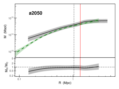
(aj)

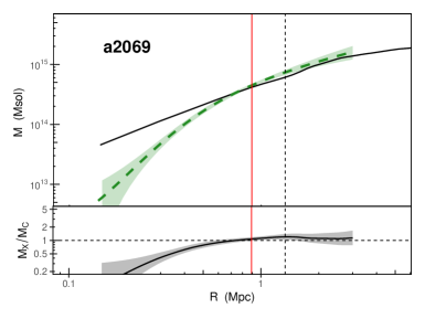
(ak)

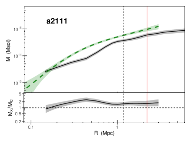
(al)

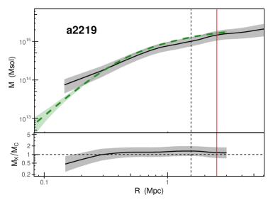
(am)

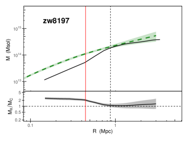
(an)

Figure 10: - continued

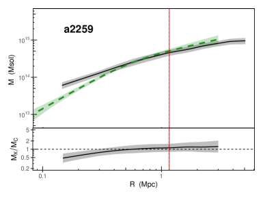
(ao)

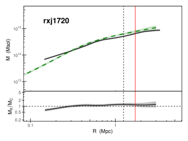
(ap)

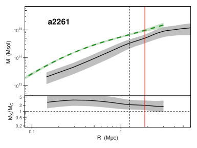
(aq)

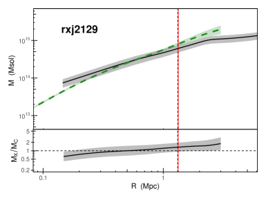
(ar)

Figure 10: - continued