Heuristic Adaptability to Input Dynamics for SpMM on GPUs

Abstract.

Sparse Matrix-Matrix Multiplication (SpMM) has served as fundamental components in various domains. Many previous studies exploit GPUs for SpMM acceleration because GPUs provide high bandwidth and parallelism. We point out that a static design does not always improve the performance of SpMM on different input data (e.g., ¿85% performance loss with a single algorithm). In this paper, we consider the challenge of input dynamics from a novel auto-tuning perspective, while following issues remain to be solved: (1) Orthogonal design principles considering sparsity. Orthogonal design principles for such a sparse problem should be extracted to form different algorithms, and further used for performance tuning. (2) Nontrivial implementations in the algorithm space. Combining orthogonal design principles to create new algorithms needs to tackle with new challenges like thread race handling. (3) Heuristic adaptability to input dynamics. The heuristic adaptability is required to dynamically optimize code for input dynamics.

To tackle these challenges, we first propose a novel three-loop model to extract orthogonal design principles for SpMM on GPUs. The model not only covers previous SpMM designs, but also comes up with new designs absent from previous studies. We propose techniques like conditional reduction to implement algorithms missing in previous studies. We further propose DA-SpMM, a Data-Aware heuristic GPU kernel for SpMM. DA-SpMM adaptively optimizes code considering input dynamics. Extensive experimental results show that, DA-SpMM achieves 1.26$\times$$\sim$1.37$\times$ speedup compared with the best NVIDIA cuSPARSE algorithm on average, and brings up to 5.59$\times$ end-to-end speedup to applications like Graph Neural Networks.

1. Introduction

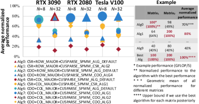
Figure 1. The left part shows the average normalized performance of different SpMM algorithms in cuSPARSE (cusparse, ) (to the algorithm with the best performance, using the geometric mean on the SuiteSparse (davis2011university, )), $N$ is the width of the dense matrix. The right part shows an example of how the average normalized performance is calculated for 2 matrices.

Sparsity is a key enabler of future Artificial Intelligence (low2012distributed, ; xiao2017tux2, ; han2015deep, ). Sparsity enables fast and energy-efficient training and inference in various domains (eie, ; mobilenets, ; sanh2020movement, ; fedus2021switch, ). However, sparse computation loses to its dense counterpart in terms of throughput, especially on throughput-oriented architectures like GPUs. In many emerging applications such as Graph Neural Networks (GNNs)(gespmm, ), recommendation (Asgari2021FAFNIRAS, ) and large language models (wang2019structured, ), Sparse Matrix-Matrix Multiplication (SpMM) has served as fundamental components and dominated total execution time (gespmm, ; eie, ). SpMM can be formulated by the multiplication between a sparse matrix and a dense matrix, exposing high potential parallelism and requires high throughput, thus many previous studies focus on accelerating SpMM using GPUs (aspt, ; jiang2020novel, ; gespmm, ; sputnik, ; wang2020sparsert, ).

However, improving the performance of SpMM suffers from the challenge of handling the input dynamics, i.e., the performance is dependent on not only the static code optimizations, but also the dynamic input characteristics. We test the performance of 10 SpMM algorithms in NVIDIA cuSPARSE (cusparse, ) on different sparse matrices (956 matrices in the SuiteSparse (davis2011university, ) dataset) and different width of the dense matrix ($N=8$ and $N=32$). Figure 1 shows performances of ten algorithms normalized to the best algorithm for each matrix. A single algorithm cannot always achieve the best performance on different input data, and the maximum performance loss with a single algorithm is ¿85% (e.g., Alg8, $N=32$ on RTX 3090). Despite its importance and obvious difficulty, tackling input dynamics is missing from the focus of previous work. For example, GE-SpMM (gespmm, ) adopts techniques like thread coarsening and shared memory to optimize the performance when $N$ is large. However, GE-SpMM is slower than cuSPARSE when $N$ is small (e.g., running GraphSAGE (graphsage, ), $N$=16, in GE-SpMM’s paper). Another example is that the thread coarsening technique cannot always achieve benefit on different data (Figure 8 in GE-SpMM’s paper).

Observing that previous work limits their optimizations to some specific scenarios, we ask this question: how can we design a generally good SpMM kernel for all kinds of scenarios? Our answer is that not a single design, but the careful composition and adaptive usage of many designs, can well address input dynamics. Previous work has proposed many ad-hoc optimizations with limited rule-based selection models. In this paper, we seek to propose design-composition-guided new optimizations, and use data-driven ML models to make input-dynamic choices of implementations. We also solve the following challenges: (1) Orthogonal design principles considering sparsity. Optimizations in dense problems consider little of sparsity in SpMM. We need to extract orthogonal design principles considering sparsity to form algorithms for auto tuning. (2) Nontrivial implementations in the algorithm space. Combining techniques (e.g., workload balance for unbalanced matrices (graphblas, ) and parallel reduction to utilize idle GPU threads (bell2009implementing, )) can bring benefits to specific inputs, while implementing them is nontrivial and missed in previous studies. (3) Heuristic adaptability to input dynamics. An efficient heuristic model is required to be adaptive to input dynamics. We make following contributions in this paper:

• We propose three sparsity-unique design principles for SpMM on GPUs. We decompose the mathematical formulation of the SpMM, with orthogonal design principles specially for sparse problems. We propose 8 algorithms according to 3 dimensions in the space, which not only cover previous designs, but also come up with new designs which are not studied.

• We propose nontrivial techniques to complete the algorithm space. We propose several techniques complete missing algorithms in the space. For example, we introduce the conditional reduction to implement workload balance for imbalance matrices and parallel reduction to utilize idle GPU threads.

• We design a data-aware kernel, DA-SpMM, to be adaptive to input dynamics. DA-SpMM considers input dynamics, and dynamically selects a design with better performance for SpMM. DA-SpMM improves the performance of a static design from $<$70% to $>$98% (normalized to the best design on each dataset).

DA-SpMM achieves 1.26$\times$$\sim$1.37$\times$ speedup on average compared with the best NVIDIA cuSPARSE algorithm, and brings up to 5.59$\times$ end-to-end speedup to applications like Graph Neural Networks.

2. Related Works

2.1. Design Principles for Sparse

TVM (chen2018tvm, ) uses affine-loop transformation which describes orthogonal design principles for dense tensor operations. Such a framework cannot handle sparse tensor operations with input-dependent loop boundaries. TACO (taco, ) proposes the sparse iterations space and a set of transformation primitives to support tuning. Unfortunately, TACO fails to consider some key techniques (e.g., parallel reduction and GPU shared memory) in their current framework, losing big room for optimization.

2.2. SpMM Optimization Techniques

Bell et al. (bell2009implementing, ) proposed a set of GPU SpMV implementations including Scalar-CSR and Vector-CSR, and the latter one can utilize idle GPU thread with a parallel reduction technique. GraphBLAS (graphblas, ) and GE-SpMM (gespmm, ) extend Scalar-CSR to SpMM scenario. CSR-Stream (greathouse2014efficient, ) and MergePath (merrill2016merge, ) handles workload balancing by introducing corresponding techniques, which work well for sparse matrices with the skewed row-length distribution. However, none of these works enable parallel reduction for SpMM and even combine parallel reduction with workload balance for skewed matrices on GPUs with high parallelism.

2.3. Input-Adaptive Kernel Selection

Choi et al. (choi2010model, ) searches for optimal format and different binning strategies. Such heuristics over-simplify input dynamics to one or a few features. Nisa et al. (Nisa2018, ) explores various ML models for format selection of sparse tensor kernels. SpTFS (10.5555/3433701.3433724, ) explores deep learning to select a sparse tensor format. No prior work has studied machine learning techniques for general SpMM tuning.

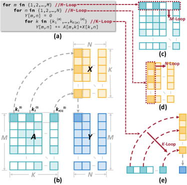
Figure 2. An overview of the SpMM. (a) Pseudo-code of SpMM with 3 loops. (b) Define SpMM as $A_{M\times K}\cdot X_{K\times N}=Y_{M\times N}$. (c) $M$-loop: Traversing rows of $A$. (d) $N$-loop: Traversing columns of $X$. (e) $K$-loop: Traversing non-zeros in $A$ and corresponding elements in $X$.

3. Design Principles for SpMM on GPUs

3.1. Three-Loop for SpMM

We explore the SpMM problem by digging into three loops of the typical SpMM implementation shown in Figure 2(a). In general, we do not introduce detailed concepts of GPUs when explaining three loops. We use the concept of worker to represent parallel processing units (e.g., threads, warps, and etc.) on GPUs.

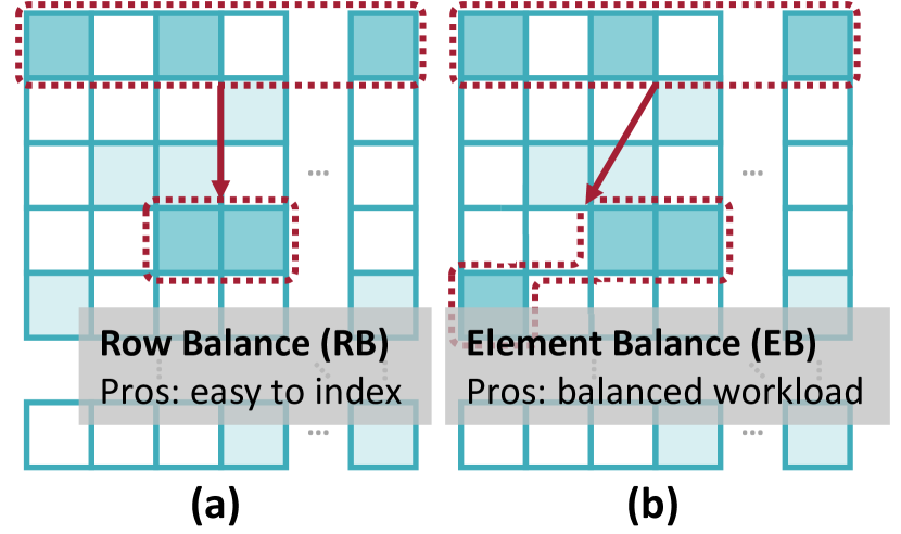
Figure 3. $M$-loop. (a) Row Balance (RB): assigning a row to a worker. (b) Element Balance (EB): assigning a given number of elements to a worker.

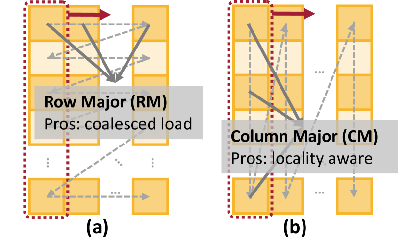
Figure 4. $N$-loop. (a) Row Major (RM): storing $X$ in the row-oriented order. (b) Column Major (CM): storing $X$ in the column-oriented order.

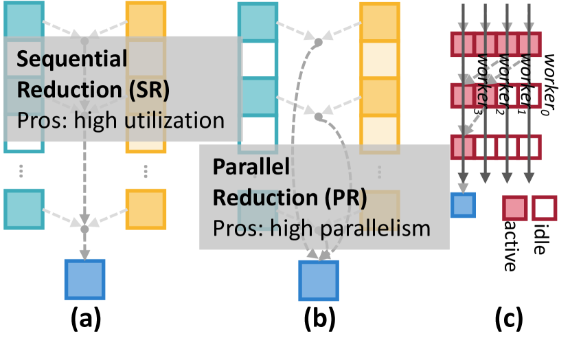
Figure 5. $K$-loop. (a) Sequential Reduction (SR): adding products sequentially.

3.2. $M$-Loop: Workload Balance

Intuition. Consider the first loop, $M$-Loop, of SpMM shown in Figure 2(a). $M$-Loop iterates over the rows of the sparse matrix $A$. For each row, the task is to multiply the non-zero elements with the dense elements they point to and accumulate results. If the $m$-th row contains $K_{(m)}$ non-zeros, $K_{(m)}\cdot N$ multiply-add operations are involved. The workload is thus specified for a given $m$ in $1\sim M$.

Design M1: Row Balance (RB). A simple way for $M$-Loop unrolling and parallel worker assignment is to assign a given number of rows to a worker, which is commonly used in dense problems. Figure 5(a) shows a simple example of the RB method by assigning one row to a worker. By adopting this RB method, we can easily get the row index of each non-zero referring to the worker index. However, workloads of different workers are imbalanced because non-zeros vary in different rows.

Design M2: Element Balance (EB). Another way to unroll $M$-Loop is the fine-grained parallelism by assigning a given number of non-zeros in the sparse matrix $A$ to a worker, which is specially for sparse problems. Figure 5(b) shows an example of the EB method by evenly distributing non-zeros to different workers, where workloads are balanced. However, such a method introduces extra overheads including calculating the row index for a non-zero and partial sum aggregation among different workers in a row.

Analysis. Compared with the RB method, the EB method balances workloads by introducing extra calculations during runtime. Thus, the RB method is supposed to achieve a better performance when the number of non-zeros in different rows is balanced. On the contrary, the EB method tends to be used when workloads become more imbalanced. We later show the controlled experiment on how workload balance affects the choice of RB and EB in Section 6.3.

3.3. $N$-Loop: Dense Matrix Access Pattern

Intuition. $N$-Loop iterates over the columns of the dense matrix $X$. Different workers process different columns of $X$ according to sparse elements in a given row of $A$ when $m$ is specified in Section 3.2. Note that workers access specific rows in parallel, thus the bandwidth efficiency caused by the memory access pattern is related to the data layout of the dense matrix $X$.

Design N1: Row Major (RM). We first consider the situation to store the dense matrix in a Row Major (RM) way, elements in a row of $X$ are stored in the contiguous memory space. Because different workers process the same rows (shown in Figure 2), the RM layout leads to coalesced memory access pattern (gespmm, ). However, such a data layout suffers from the poor locality for one worker because several rows are skipped, shown in Figure 5(a).

Design N2: Column Major (CM). Another data layout is to store $X$ using a Column Major (CM) order, shown in Figure 5(b). Compared with the RM layout, less memory space is skipped for a worker when processing two neighbor non-zeros in a column, which is beneficial to locality. However, parallel workers cannot benefit from coalesced memory access patterns because data in a row are not stored contiguously, shown in Figure 5(b).

Analysis. Note that the initial and final layout need to be aligned to the previous and next kernel in the application, thus often fixed, we have control on the intermediate matrix layout. When $N$ is small, the RM layout suffers from poor locality because several rows are skipped, while the CM major benefits from locality if the non-zero coordinates $k$’s appear close to each other. However, when $N$ is large, the RM layout shows advantage over CM because it exploits coalesced loading of a row of $X$, which increases the amount of effective data per request and improves bandwidth efficiency. We can easily infer that the parameter $N$ affects the performance of RM and CM for specific sparse matrices. We also show the controlled experiment on the choice of RM and CM in Section 6.3.

3.4. $K$-Loop: Parallelism Efficiency

Intuition. At last is the third loop, $K$-Loop. In this loop, non-zero elements of a row in $A$ and corresponding elements of a column in $X$ are traversed to calculate the inner product. Note that this loop requires a reduction operation among element pairs to get the sum, the efficiency of parallel workers is related to the way to implement such a reduction operation.

Design K1: Sequential Reduction (SR). A simple way to implement this reduction operation is to assign one worker to calculate the sum and perform the Sequential Reduction (SR) method, shown in Figure 5(a). The SR method achieves high utilization of workers because each worker is always busy when during reduction, which is often used for computation-bounded dense problems. However, such a method loses the potential parallelism existing in the reduction for sparse problems.

Design K2: Parallel Reduction (PR). Another implementation takes the potential parallelism existing in this reduction operation, as is shown in Figure 5(b). We call this method Parallel Reduction (PR), which has been used for sparse problems like Sparse Matrix-Vector Multiplication problems in (bell2009implementing, ). Compared with SR, PR exploits the potential parallelism in reduction, and a typical implementation of PR is a merge-tree shown in Figure 5(d). However, PR suffers from poor utilization of workers because several workers are idle during the reduction, shown in Figure 5(c).

Analysis. The SR and PR methods show two ways of assigning the $K$-Loop to workers. In Figure 5(c), the PR method achieves higher parallelism while the efficiency/utilization of each parallel worker is lowered. When processing larger matrices, the parallelism lost by SR can be compensated by processing more reduction operations in parallel, and the performance tends to be better than the PR method due to higher utilization. On the contrary, PR tends to be better when processing smaller matrices (or GPUs with higher parallelism). The reason is that SR cannot fully utilize the parallelism provided by the GPU. Thus, the performance comparison between the SR and PR methods is closely related to the data size.

Table 1. Summary of previous works in the algorithm space

$M$-Loop	RB	RB	RB	RB	EB	EB	EB	EB
$N$-Loop	RM	RM	CM	CM	RM	RM	CM	CM
$K$-Loop	SR	PR	SR	PR	SR	PR	SR	PR
RowSplit(graphblas, )	✓
MergeSpMM(graphblas, )	✓
ASpT(aspt, )					✓
GE-SpMM(gespmm, )	✓
Ours	✓	✓	✓	✓	✓	✓	✓	✓

3.5. Comparison with Previous Works

Based on the novel three-loop model, we summarize previous SpMM designs in Table 1. By decomposing the mathematical formulation of SpMM, combining design principles is capable of covering all previous designs. Moreover, we can also find new designs for the SpMM (e.g., RB+RM+PR.). We implement all 8 designs based on these design principles, which are further used for performance tuning in later sections.

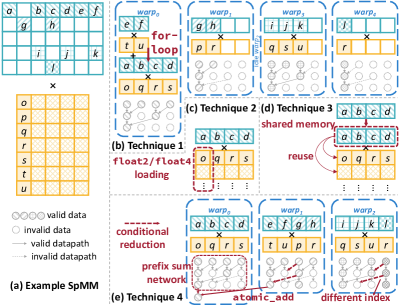
Figure 6. Implementations of different SpMM algorithms under the algorithm space with proposed techniques, number of threads in a warp is 4. (a) An example of SpMM with legends in latter subfigures. (b) Using for-loop to reduce $>4$ elements for RB. (c) Using float2/float4 to load multiple dense elements for RM. (d) Using shared memory to cache sparse elements for reuse. (e) Using a prefix sum network with conditional reduction for EB.

4. Implementations

As mentioned in Table 1, previous studies on SpMM only explore both RB and EB methods for the $M$-Loop, while CM for the $N$-Loop and PR for the $K$-Loop is lacking. Implementing CM is trivial derived from the implementation of the corresponding RM design by storing the dense matrix in a column-oriented order. Thus, we can easily get RB+CM+SR and EB+CM+SR from current implementations.

RB+RM+PR. The main challenges of implementing PR under RB include: (1) The number of elements to perform the reduction may be larger than the number of threads in a GPU warp, thus the reduction cannot be processed within one warp instruction. (2) Different columns require same non-zeros in a row of the sparse matrix, leading to redundant data loading. Figure 6(a) shows an example of performing reduction on 5 sparse rows with 6/2/0/3/1 non-zeros each row, we set the number of threads in a warp to 4. We utilize a for-loop (Technique 1) in Figure 6(b), for the first challenge to enable reduction of $>$4 (number of threads in a warp) elements (e.g., the first row). For the second challenge, we utilize float2/float4 (Technique 2), shown in Figure 6(c), primitive to load multiple elements in consecutive columns in the dense matrix, and these columns are processed by a warp. However, the float2/float4 primitive only enables us to process at most 4 columns within a warp. In order to reuse data for large $N$ (columns in the dense matrix), we further utilize shared memory (Technique 3), shown in Figure 6(d), to cache sparse elements for different columns. Thus, these elements can be reused for multiple columns.

EB+RM+PR. The main challenges of implementing PR under EB include: (1) A warp needs to perform reduction on different rows for the same number of elements in the sparse matrix. (2) The same challenge as the second challenge in RB+RM+PR, thus Technique 2/3 can still be used. Inspired by the prefix sum network, we propose the conditional reduction (Technique 4), shown in Figure 6(e), method to solve the first challenge. Besides the partial reduction result, a thread records a index flag to distinguish the row. For each reduction step, the datapath of the prefix sum network is activated if two threads share the same index flag. The outputs of such a conditional prefix sum network are valid for the first (leftest) thread or the thread with different index compared with the thread on its left. For rows assigned to different warps, an atomic_add operation is performed get the final reduction result.

RB+CM+PR. The only difference to RB+RM+PR is that the dense matrix is stored in a column-oriented order, thus Technique 2 cannot be used because elements in a row are not stored consecutively, while Technique 1/3 are applied.

EB+CM+PR. Similar to RB+CM+PR, Technique 2 is not applied, while Technique 3/4 in EB+RM+PR are used.

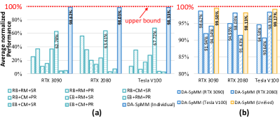
Figure 7. Average normalized performance of the heuristic DA-SpMM kernel. (a) DA-SpMM based on features of input data against 8 static designs proposed in Section 3. (b) A unified DA-SpMM kernel for different GPUs.

5. Heuristic Kernels

5.1. Heuristic Adaptability

We get 8 optimized SpMM algorithms in Section 4, and we also analyze that characteristics of the input data affect the performance of implementations. Then, we further test the performance of all these 8 designs on 3 different GPUs with 956 matrices in the SuiteSparse dataset (with detail setups in Section 6.1). The average normalized performance (the meaning is the same as that in Figure 1) is shown in Figure 7(a). We can get the same conclusion that a single algorithm cannot always achieve the best performance on different input data, and a single algorithm with the best average normalized performance is $<$70%.

Thus, to be adaptive to input dynamics and achieve a better performance, auto tuning has been proved as an effective method. We leverage the gradient boosting framework LightGBM (lightgbm, ) to train a prediction model to select the best design from the 8 different designs. We select a collection of features extracted from both the sparse matrix and the dense matrix as the input vector to our model, as in Table 2.

Table 2. Extracted features in heuristic kernels.

Feature	Meaning
nnz	Number of non-zeros in the sparse matrix
mat_size	Size of the sparse matrix
std_row	Standard deviation of non-zeros in rows
N	Width of the dense matrix

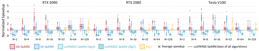
Figure 8. SpMM performance comparison among our DA-SpMM, GE-SpMM (gespmm, ), and ASpT (aspt, ), and cuSPARSE (cusparse, ).

5.2. Evaluation

5.2.1. Individual Model.

We also use the average normalized performance as the criterion to evaluate the performance of our heuristic kernel, DA-SpMM. Here we train three individual models for each GPU. We set the ratio of train, validation, and test data to 40%, 10%, and 50%, respectively. As is shown in Figure 7(a), DA-SpMM achieves 98.62%, 98.03%, and 98.33% normalized performance on 3 GPUs (an average of 98.33%), respectively. In contrast, the best normalized performance of one static design is lower than 70%.

5.2.2. Unified Model.

We further test the performance of migrating the model trained by one GPU to another, leading to an average of 5.38% performance loss (e.g., using DA-SpMM model trained by RTX 2080, i.e., DA-SpMM (RTX 2080), for Tesla V100 degrades the performance from 98.33% to 90.64%). To be adaptive to different GPUs, we further distinct different GPUs to train one unified LightGBM model. The result shows that, a unified DA-SpMM can not only solve the performance loss of migrating the model, it also further achieves the better performance, 99.50%, 98.13%, and 99.17% on 3 GPUs (an average of 98.93%).

5.3. Heuristic Kernel Conclusion

By introducing the heuristic model to dynamically select kernels with better performance, DA-SpMM is adaptive to input dynamics. With only data features for model training, DA-SpMM improves the normalized performance from less than 70% to over 98% for different GPUs. By introducing hardware features, DA-SpMM further improves the performance with a unified heuristic model.

6. Experimental Results

6.1. Experimental Setup

6.1.1. Environments.

We use three different GPUs set up our experimental environments for previous and this sections:

NVIDIA RTX 3090. Compute Capability 8.6 (68 Ampere SMs at 1.395 GHz, 24 GB GDDR6x, 936 GB/s bandwidth).

NVIDIA RTX 2080. Compute Capability 7.5 (46 Turing SMs at 1.515 GHz, 8 GB GDDR6, 448 GB/s bandwidth).

NVIDIA Tesla V100. Compute Capability 7.0 (80 Volta SMs at 1.370 GHz, 16 GB HBM2, 900 GB/s bandwidth).

6.1.2. Baselines.

GE-SpMM (gespmm, ) is a state-of-the-art open-source SpMM design on GPUs, it achieves better performance against other open-source design like GraphBLAST (graphblast, ).

ASpT (aspt, ) adopts a matrix tiling preprocessing step to process dense and sparse sub-matrix separately during runtime. We only count the execution time of ASpT while excluding the preprocessing time. Moreover, ASpT only supports $N=32$ and $N=128$ cases.

NVIDIA cuSPARSE (cusparse, ) is a vendor library by NVIDIA. We use the routine cusparseSpMM for SpMM, we use version 11.2.

All results are normalized to the best cuSPARSE algorithm for each matrix. All codes are compiled using nvcc 11.2 with -O3 flag.

6.1.3. Datasets.

We use SuiteSparse collection (davis2011university, ) with 956 matrices (We use the script of ASpT (aspt, ) to select these matrices which removes isomorphic one to enable diversity) to test performance.

6.2. Performance of Heuristic Kernel

We compare the DA-SpMM design with GE-SpMM (gespmm, ), ASpT (aspt, ), and two cuSPARSE (cusparse, ) SpMM algorithms (Alg3 and Alg7 in Figure 1, which are two best static algorithms). All results are normalized to the best cuSPARSE SpMM algorithm on each matrix, shown in Figure 8. We can get following conclusions:

Against the static cuSPARSE algorithm. For different $N$ from 2 to 128, DA-SpMM achieves an average speedup of up to 2.96$\times$, 2.66$\times$, 2.57$\times$ on three GPUs, respectively.

Against different cuSPARSE algorithms with the best performance on each matrix. For different $N$ from 2 to 128, DA-SpMM achieves an average speedup of 1.37$\times$, 1.26$\times$, and 1.30$\times$ on three GPUs, respectively. For large $N$ (e.g., $N=128$), DA-SpMM achieves higher speedup of 1.60$\times$, 1.36$\times$, and 1.30$\times$, respectively.

Against ASpT. For $N=32$, DA-SpMM achieves an average speedup of 1.14$\times$, 1.14$\times$, and 1.06$\times$, respectively. For $N=128$, the speedup is 1.20$\times$, 1.14$\times$, and 1.05$\times$. The preprocessing time of ASpT is not counted.

Against GE-SpMM. DA-SpMM achieves significant improvements for small $N$ (4.99$\times$, 5.23$\times$, and 5.40$\times$ for $N=2$). When $N$ becomes larger, the performance of GE-SpMM improves. For $N=128$, the speedup against GE-SpMM is 1.29$\times$, 1.04$\times$, and 1.59$\times$ on three GPUs, respectively. When $N$ becomes larger, DA-SpMM prefers to select RM for $N$-loop and SR for $K$-loop in most cases. These two selections are the same with the design in GE-SpMM, which means that GE-SpMM does reach the optimal design point for these cases, except for the balance design in the $M$-loop.

6.3. Controlled Experiments

As we have analysed in Section 3, the choice of different algorithm for each loop depends on input dynamics. Thus, we synthesize matrices and conduct controlled experiments.

6.3.1. RB-EB

We take three sparse matrices with identical size and sparsity, but different $std\_nnz$, i.e., the standard deviation of the number of non-zeros in each row. The matrices are synthesized R-MAT graphs  (chakrabarti2004r, ) by tuning parameters related to element distribution. The result is shown in Figure 9(a). The EB method exceeds the RB method as the standard deviation of non-zeros in each row grows, because the imbalance among different workers becomes the main factor for the performance difference.

6.3.2. RM-CM

We synthesize one same sparse matrix with three different dense matrices, with R-MAT method (chakrabarti2004r, ). We vary $N$ for the dense matrix. The result is shown in Figure 9(b). The RM layout achieves higher performance against the CM layout when $N$ gets larger. The reason is that larger $N$ leads to coalesced load for different workers. In contrast, the CM implementation always needs to skip elements in the dense vector, thus the effective data per request is inherently limited.

6.3.3. SR-PR

We synthesize three matrices with the same sparsity and non-zero distribution, but different non-zeros, with R-MAT method (chakrabarti2004r, ). The bars in Figure 9(c) display non-zeros of each matrix, and the lines plot the relative performance of SR against PR. When the matrix is small, the PR method is better than the SR method because it saturates parallelism, but SR gains advantages when the matrix size gets larger because the utilization of one worker becomes the main factor for the performance.

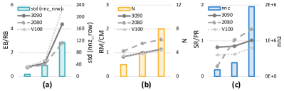
Figure 9. Controlled experiments to show how input data dynamics affect choice of different algorithms for each loop. (a) RB-EB: workload balance. (b) RM-CM: data access pattern. (c) SR-PR: total workloads.

6.4. Performance of Heuristic Kernel in GCNs

We integrate DA-SpMMul into the Graph Neural Network framework, DGL (dgl, ), to compare the end-to-end performance on RTX 3090 with GCN (kipf2016semi, ) and GraphSAGE (graphsage, ) models. We test the inference speedup with on the Reddit dataset (reddit, ), in Figure 10. By using DA-SpMM, we achieve up to 5.59$\times$ and 5.27$\times$ speedup against the original DGL framework on two GNN models, respectively.

7. Conclusions

In this paper, we present a thorough study of Sparse Matrix-Matrix multiplication (SpMM) on GPUs. We consider the SpMM acceleration problem from a novel auto-tuning perspective to be adaptive to input dynamics. We first propose a novel three-loop model with orthogonal design principles specially for sparse problems. We also propose several techniques to implement new designs which are not previously studied. We further propose DA-SpMM to adaptively optimize code and achieve a better performance considering input dynamics. Evaluations show that DA-SpMM is the fastest among commercial and academic designs: DA-SpMM achieves an average of 1.26$\times$$\sim$1.37$\times$ speedup compared with the best NVIDIA cuSPARSE algorithm, and brings up to 5.59$\times$ end-to-end speedup to applications like Graph Neural Networks. Our methodology of composing design principles into an algorithm space and using heuristic models for algorithm selection can be extended to further studies on sparse acceleration problems.

Figure 10. Performance comparison for GNNs. X-axis: feature length. Y-axis: Normalized speedup (to the original framework using cuSPARSE). (a) GCN. (b) GraphSAGE.

8. Acknowledgements

The design in this paper will be included in our dgSPARSE project.

References

- [1] Basic linear algebra for sparse matrices on nvidia gpus. =https://developer.nvidia.com/cusparse.
- [2] Scott P. Kolodziej et al. The suitesparse matrix collection website interface. Journal of Open Source Software, 4(35):1244, 2019.
- [3] Yucheng Low et al. Distributed graphlab: A framework for machine learning in the cloud. arXiv :1204.6078, 2012.
- [4] Wencong Xiao et al. Tux2: Distributed graph computation for machine learning. In NSDI, pages 669–682, 2017.
- [5] Song Han et al. Deep compression: Compressing deep neural networks with pruning, trained quantization and huffman coding. arXiv :1510.00149, 2015.
- [6] Song Han et al. Eie: Efficient inference engine on compressed deep neural network. In ISCA, pages 243–254, 2016.
- [7] Andrew G Howard et al. Mobilenets: Efficient convolutional neural networks for mobile vision applications. arXiv :1704.04861, 2017.
- [8] Victor Sanh et al. Movement pruning: Adaptive sparsity by fine-tuning. arXiv :2005.07683, 2020.
- [9] William Fedus et al. Switch transformers: Scaling to trillion parameter models with simple and efficient sparsity. arXiv :2101.03961, 2021.
- [10] Guyue Huang et al. Ge-spmm: general-purpose sparse matrix-matrix multiplication on gpus for graph neural networks. In SC, pages 1–12, 2020.
- [11] Bahar Asgari, Ramyad Hadidi, Jiashen Cao, Da Eun Shim, Sung Kyu Lim, and Hyesoon Kim. Fafnir: Accelerating sparse gathering by using efficient near-memory intelligent reduction. HPCA, pages 908–920, 2021.
- [12] Ziheng Wang, Jeremy Wohlwend, and Tao Lei. Structured pruning of large language models. arXiv :1910.04732, 2019.
- [13] Changwan Hong et al. Adaptive sparse tiling for sparse matrix multiplication. In PPoPP, pages 300–314, 2019.
- [14] Peng Jiang et al. A novel data transformation and execution strategy for accelerating sparse matrix multiplication on gpus. In PPoPP, pages 376–388, 2020.
- [15] Trevor Gale et al. Sparse gpu kernels for deep learning. In SC, pages 1–14, 2020.
- [16] Ziheng Wang. Sparsert: Accelerating unstructured sparsity on gpus for deep learning inference. In PACT, pages 31–42, 2020.
- [17] William L Hamilton et al. Inductive representation learning on large graphs. In NeurIPS, pages 1025–1035, 2017.
- [18] Carl Yang et al. Design principles for sparse matrix multiplication on the gpu. In Euro-Par, pages 672–687. Springer, 2018.
- [19] Nathan Bell and Michael Garland. Implementing sparse matrix-vector multiplication on throughput-oriented processors. In SC, pages 1–11, 2009.
- [20] Tianqi Chen et al. Tvm: An automated end-to-end optimizing compiler for deep learning. In OSDI, pages 578–594, 2018.
- [21] Fredrik Kjolstad et al. Taco: A tool to generate tensor algebra kernels. In ASE, pages 943–948, 2017.
- [22] Joseph L Greathouse and Mayank Daga. Efficient sparse matrix-vector multiplication on gpus using the csr storage format. In SC, pages 769–780, 2014.
- [23] Duane Merrill and Michael Garland. Merge-based parallel sparse matrix-vector multiplication. In SC, pages 678–689, 2016.
- [24] Jee W Choi et al. Model-driven autotuning of sparse matrix-vector multiply on gpus. ACM Sigplan Notices, 45(5):115–126, 2010.
- [25] Israt Nisa et al. Effective machine learning based format selection and performance modeling for SpMV on GPUs. IPDPSW, pages 1056–1065, 2018.
- [26] Qingxiao Sun et al. Sptfs: Sparse tensor format selection for mttkrp via deep learning. In SC, 2020.
- [27] Lightgbm. https://lightgbm.readthedocs.io/en/latest/.
- [28] Carl Yang et al. Graphblast: A high-performance linear algebra-based graph framework on the gpu. arXiv :1908.01407, 2019.
- [29] Deepayan Chakrabarti et al. R-mat: A recursive model for graph mining. In ICDM, pages 442–446, 2004.
- [30] Minjie Wang et al. Deep graph library: A graph-centric, highly-performant package for graph neural networks. arXiv :1909.01315, 2019.
- [31] Thomas N Kipf and Max Welling. Semi-supervised classification with graph convolutional networks. arXiv :1609.02907, 2016.
- [32] William L Hamilton et al. Reddit dataset in graphsage. website, 2017. http://snap.stanford.edu/graphsage/.